

Development and Application of a Coastal Change Likelihood Assessment for the Northeast Region, Maine to Virginia
Links
- Document: Report (26.8 MB pdf) , HTML , XML
- Data Release: USGS data release - Coastal change likelihood in the U.S. northeast region—Maine to Virginia
- Download citation as: RIS | Dublin Core
Acknowledgments
This research was done in cooperation with Natural Resource Preservation Program of the National Park Service. This study benefited from meetings, thoughtful conversations, and user engagement with Amanda Babson, James Nyman, and numerous National Park Service archeologists and staff. Summer interns Nora Hyman, Tyvonta Johnson, and Mya Rufus also helped support aspects of this research either through accuracy assessment or land cover research, and we are grateful for their contributions. This manuscript benefited from conversations and input from the Estuarine Dynamics Team at the Woods Hole Coastal and Marine Science Center of the U.S. Geological Survey.
Abstract
Coastal resources are increasingly affected by erosion, extreme weather events, sea level rise, tidal flooding, and other potential hazards related to climate change. These hazards have varying effects on coastal landscapes because of the compounding of geologic, oceanographic, ecologic, and socioeconomic factors that exist at a given location. An assessment framework is introduced in this report that synthesizes existing datasets that cover the variability of the landscape, and hazards that may act on the landscape, to evaluate the likelihood of coastal change along the U.S. coastline on a decadal scale. The pilot study that aided in the development of the framework was run in the northeastern United States (from Maine to Virginia) and consists of datasets derived from a variety of Federal, State, and local sources.
First, a decision-tree-based dataset was built that describes the resistance or integrity of the coastal landscape (called the fabric dataset for the purposes of this report) and includes land cover, elevation, slope, long-term (more than 50 years) shoreline change, dune height, and marsh stability data. A second database was generated from coastal hazards, which are divided into event hazards (for example, flooding, wave power, and probability of storm overwash) and persistent or perpetual hazards (for example, relative sea level rise rate, short-term [about 30-year] shoreline erosion rate, and storm recurrence interval). The fabric dataset was then merged with the coastal hazards databases, and a model training dataset made up of hundreds of polygons was generated from these combined data to support machine learning.
The pilot study resulted in location-specific, 10-meter-resolution data classified into five raster datasets that include intrinsic characteristics of the coast used to determine the resistance of the landscape to change, the persistent and event hazards that act on the coast, the machine learning output (coastal change likelihood) based on the cumulative effects of the fabric and hazards datasets, and an estimate of the hazard type (event or persistent) that is the most likely to influence coastal change. Final outcomes are intended to be used as a first-order planning tool to determine which areas of the coast are more likely to change in response to future potential coastal hazards and to examine elements and drivers that make change in a location more likely.
1. Introduction
Coastal change is a product of the dynamic response to natural hazards such as storm events and sea level rise and is essential to the ecological function and morphologic evolution of modern coastal landscapes. As coastal populations grow, the effects of coastal change—erosion, flooding, and inundation, all of which may lead to land loss—present a variety of threats to coastal communities and cities, critical habitat, infrastructure, and cultural and natural resources (Neumann and others, 2015). Furthermore, as the full potential of climate change is realized, natural hazards are expected to increase in frequency and become more extreme in coming years (Dupigny-Giroux and others, 2018; Intergovernmental Panel on Climate Change, 2021). Understanding where coastal change is most likely to occur provides essential information to help managers and planners prepare for future vulnerabilities to people and resources.
The U.S. Geological Survey (USGS) and the National Park Service have developed a methodology for a comprehensive regional-scale assessment of expected landscape change during the next decade to support resource preservation in coastal park units. Partnering with the National Park Service, through the USGS Natural Resources Preservation Program, a pilot study is outlined in this report for the northeastern United States where a variety of coastal change hazards threaten archeological and cultural resources in the region. Although the outcomes of the pilot study are intended for direct application to archeological resource issues, the scale, scope, and focus of this study on the integrity of the landscape in response to natural hazards is broadly applicable for assessing climate change effects in the coastal zone at the decadal scale. The outcomes of this study provide an important enhancement to the USGS coastal vulnerability index (CVI) to sea level rise, leveraging improvements in source data and data science methods, alongside considerations of decision-support and uncertainty, to provide seamless, high-resolution data layers that can be ingested into or overlain with a variety of spatial products and assessments to inform future coastal planning.
1.1. Previous and Related Works
1.1.1. USGS Coastal Change Assessments
Coastal change likelihood (CCL) is a new USGS framework for assessing coastal change in the coming decade. It consists of three parts: the fabric, hazards, and CCL outcomes. The CCL methodology synthesizes existing geospatial datasets that describe the coastal landscape, intrinsic properties unique to landscapes, and the processes that affect the landscape, and then applies supervised machine learning to meld the landscape and hazards together, while recognizing the dependencies, complexities, uncertainties, and compounding that can occur between the landscape and hazards within the coastal zone. CCL products provide a coastal data synthesis to support decision making by highlighting areas where change is more likely, less likely, or uncertain, while acknowledging the complexity of coastal change and its prediction. Mapping out the landscape, its propensity for change, and the potential drivers of change supports decision makers tasked with preserving natural and cultural resources that may be vulnerable because of their location on the coastal landscape. The CCL framework updates and supersedes the USGS CVI assessment (Thieler and Hammar-Klose, 1999), and shares some common objectives, which include highlighting areas of the coast that may be susceptible to change from coastal hazards, incorporates available data from disparate agencies and disciplines, provides outcomes to support decision making, and is most effective at regional scales. However, since the first CVI studies (Gornitz, 1990; Shaw and others, 1998) and the first USGS CVI assessment (Thieler and Hammar-Klose, 1999), there have been improvements to availability, quality, resolution, and coverage of source datasets (table 1). Likewise, data management tools can be leveraged to assess large domains, and machine learning classification can be utilized to ingest and process greater data resolution and variability (for example, geological and ecological). Figure 1 illustrates some of these differences in CVI and CCL for an area near Cape Cod National Seashore in Massachusetts.
Table 1.
A comparison of elements of the U.S. Geological Survey coastal variability index study and the coastal change likelihood framework.[The U.S. Geological Survey (USGS) coastal variability index (CVI) study is from Thieler and Hammar-Klose (1999). The coastal change likelihood (CCL) framework is detailed in this report, and the data are from Sterne and others (2023)]
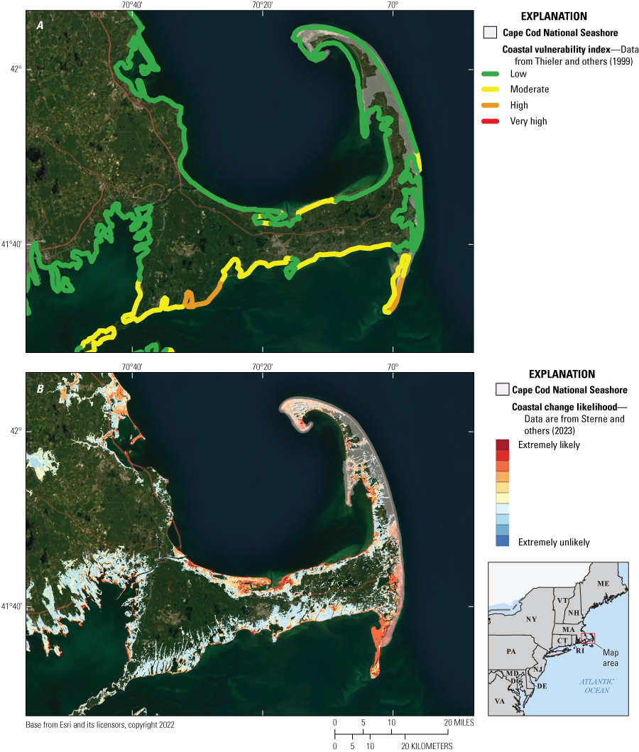
Maps showing results of the coastal vulnerability index and coastal change likelihood (CCL) at Cape Cod National Seashore and Cape Cod, Massachusetts, as part of assessments of coastal change on the Northeast Atlantic Coast. A, The U.S. Geological Survey (USGS) coastal vulnerability index (CVI) dataset for the Atlantic Coast displayed for an area along southeastern Massachusetts; the CVI dataset is from Thieler and Hammar-Klose (1999). B, The USGS CCL dataset for the northeastern United States displayed for the same area along southeastern Massachusetts; the CCL dataset is from Sterne and others (2023).
The coastal response likelihood (CRL) assessment (Lentz and others, 2015, 2016) is a related product for the CCL assessment. These data operate on the same domain, but whereas the CCL assessment focuses on coastal change as a result of landscape resistance and hazards in the next 0 to 10 years, the CRL assessment focuses primarily on sea-level-rise-related coastal change, identifying areas that are likely to become inundated as opposed to areas that are more likely to change or adapt within multidecadal intervals over the next century.
1.1.2. National Park Service Vulnerability Assessments
The CCL assessment has some overlap in methodology with the coastal facilities vulnerability assessment protocol outlined by the National Park Service in partnership with Western Carolina University (Peek and others, 2017). The National Park Service approach, first described by Glick and others (2011), has been applied to more than 20 park units and assesses vulnerability for park infrastructure and transportation assets by assimilating information on the hazards that an asset is exposed to—such as sea level rise, storm surge, flooding, and proximity to erosion—with design factors—such as structure elevation and historical damage—that determine how the asset may fare when affected by a hazard. The approach includes adaptation strategies related to asset preservation along with a measure of vulnerability that is calculated by combining the hazard exposure data with asset sensitivity information and has been effective at assessing threats to physical infrastructure within parks.
A related study addressed integrated coastal climate vulnerability of cultural, natural, and facility assets at Fire Island National Seashore (Ricci and others, 2020) and Colonial National Historical Park (Ricci and others, 2019). The objective was to create vulnerability indicator maps for the parks that focused on climate stress projections of sea level rise; flooding; erosion; drought; groundwater, precipitation, and temperature changes for a timeframe to 2050.
A shared goal of this study and the previous works of Peek and others (2017) and Ricci and others (2019) is to create decision support products for park managers that can be used to assess the hazards present across the landscape and what resources may be affected by those hazards. The unique opportunity that the CCL study presents is a seamless synthesis of coastal change factors in the Northeast, which will allow relative correlation among different park units and will highlight areas across the region with the highest propensity for near-term (decadal) coastal change.
1.2. Defining CCL–Related Terminology
The Intergovernmental Panel on Climate Change (IPCC) defines vulnerability as “the propensity of a system to be adversely affected” (Intergovernmental Panel on Climate Change, 2014). More specifically, natural resource vulnerability is defined as the extent to which a species, habitat, or ecosystem is susceptible to harm and is comprised of three elements: exposure, sensitivity, and adaptive capacity (Glick and others, 2011). In this context, exposure is a determination of whether a resource or asset is in an area experiencing climate change and other coastal hazards (for example, sea level rise, tidal flooding, erosion); sensitivity measures how a resource or asset fares when affected by a hazard, like a large storm; and adaptive capacity reflects the ability of an asset to cope or adjust in response to a hazard. The elements of Glick and others (2011) are commonly expressed and applied as an equation (Western Carolina University and National Park Service, 2016), such that
Unlike previous coastal change assessments, including the USGS CVI (Thieler and Hammar-Klose, 1999), the CCL assessment does not assign vulnerability scores; rather, the CCL assessment focuses on the exposure and sensitivity elements, where adaptive capacity is considered inherent in the landscape. Because the effects of the change on humans and ecosystems and their adaptive capacity are beyond the scope of the approach, the CCL is not considered a vulnerability assessment. Sensitivity in the CCL assessment relates to landform resistance to change or its integrity, which is defined by landscape composition, texture, aggregate stability, shear strength, and infiltration capacity on a material scale (Morgan, 2005), and the record of historical change and proximity to hazards on the landscape scale. Change in the CCL assessment pertains to the landscape rather than the assets or species found on it (for example, structural integrity or salinity tolerance, respectively). To differentiate the landscape-based classification from the often asset-based terminology described in Glick and others (2011) and subsequent vulnerability assessments, for the purposes of this report, the physical characteristics and associated metrics that define the sensitivity or propensity of the coastal environment to change (or resist change) are referred to as the fabric dataset. Exposure is a spatial determination based on whether a hazard occurs in the area—the presence or absence of a hazard acting on the landscape. Regarding effects of hazards on the landscape, change in CCL is not considered adverse or advantageous with regards to assets, livelihood, species, habitats, and ecosystems. Rather than a vulnerability assessment, CCL outcomes are expressed in likelihoods and are intended to serve as a baseline to help decision makers outline the intrinsic properties of the landscape, prioritize actions, or identify areas likely to experience adverse effects, and to inform next steps, adaptation strategies, or vulnerability assessments.
The CCL outcomes provided in this study are landscape specific and are described in terms of relative degrees of higher and lower likelihood of coastal change occurring in the coming decade. The exact physical change (table 2) depends on the landscape, ecosystems present, and transport-dependent and biogeochemical processes operating at finer spatial scales than this study can resolve or ingest (Ward and others, 2020). Prediction of the type of physical change that a landscape may undergo is beyond the scope of this study. The types of physical change that can occur across landscapes are dependent on coastal hazards and intrinsic coastal properties (for example, landform composition); for example, a forest may be classified as having a high change likelihood because it is located at a low elevation and within a zone likely to experience sea level rise flooding in the coming decade. Forested landscapes that experience sea level rise are likely to change through ecological succession, such that trees die off, become ghost forests, and are replaced by wetland habitat (Kirwan and Gedan, 2019).
Table 2.
Common coastal landscapes and possible changes or effects they may experience because of climate change and coastal hazards.[This list is not exhaustive nor indicative from an asset or ecosystem perspective. No change is a possible response in all landscape classes]
High CCL values do not always equate to landscape conversion, such as the ghost forest example above, but CCL indicates where landscapes are more likely than other areas to change in form or function based on available data. Landscape transition from one type to another, often referred to as threshold crossing, is closely linked to a landscape’s ability to resist change or adapt. For example, rocky coasts are highly resistant in response to event forcing. Common coastal hazards such as storm waves are not likely to alter a rocky shore coast within a decade, but a rise in relative sea level may inundate a low-elevation rocky shore, making landscape conversion from a rocky shore coast to an aquatic bed the singular response to sea level rise. Conversely, sandy beaches have a low resistance to forcing, but are highly resilient, such that they can recover after a storm or alter their form to adapt to a hazard. Nearly every coastal process from waves and tides to storms and sea level rise has the capacity to alter an unconsolidated beach. Beaches undergo near constant change with a diverse range of response options, including inundation, vertical or lateral erosion or accretion, or translation to another landscape such as wetland or tidal flat. Because beaches are dynamic in their response to coastal forcing, they often require site-specific knowledge, high-resolution observations, and integrated numerical modeling investigations to predict morphologic response, and still their response remains challenging to predict with temporal and spatial accuracy.
The CCL assessment provides a flexible framework that indicates where a myriad of factors that influence coastal change across a variety of landscapes exists, and those change likelihood indications can be used to inform and identify areas for further investigation from asset and resource vulnerability assessments to scientific research that targets coastal landscape response at fine scales. Further, CCL supports decision making through interdisciplinary data synthesis and analysis by providing foundational datasets for defining and mapping the complexity of factors that contribute to coastal change, community risk, and threats in the coastal environment. However, CCL should not be used to equate landscape change to asset vulnerability, indicate an imminent threat to a resource, assign risk to humans and ecosystems, or predict a physical response to forcing.
1.3. Purpose
The USGS, through its Natural Resource Preservation Program and in cooperation with the National Park Service, compiled previously published data from numerous agencies to support archeological resource management in national parks. This report presents the methodology for the CCL data layers available for download in Sterne and others (2023). The data products include the coastal fabric dataset (a summary of the coastal landscape and its intrinsic properties), the extent of event hazards, the extent of perpetual hazards, the CCL (an estimate of the likelihood to change as function of the fabric and event and perpetual hazards), and an estimate of the hazard-type (event or perpetual) that is likely to drive future change. These five datasets can be used to support near-term (decadal) decision making in the coastal zone and are intended to be used in conjunction with other data and expertise to explore vulnerabilities and potential physical changes.
1.4. Setting of the Pilot Study
This study covers the northeastern United States from the Canadian border with Maine to the border between Virginia and North Carolina. The region of interest for the CCL project is the same as the CRL model (Lentz and others, 2015) where the spatial domain is defined as the area between −10-meter (m) isobath and the +10-m contour relative to the MHW elevation (fig. 2). The data domain covers a variety of coastal settings, including open-ocean beaches, protected embayments, rocky shores and headlands, bluffs, palustrine to estuarine wetlands, urban areas (for example, Boston), and federally or privately protected lands, such as the National Park Service Cape Cod National Seashore and the Nature Conservancy Volgenau Virginia Coast Reserve. From north to south, the region transitions from a rugged and crenulated bedrock-framed shore to a gently sloping, sandy coast with marshes fronted by barrier islands. The transition in geologic framework and coastal morphology is controlled by the underlying bedrock and coastal plain, Pleistocene glaciations, and Holocene sea level rise (Emery and Uchupi, 1984). To provide focus on archaeological and cultural resource applications, five coastal national park units (fig. 2; app. 1) are used as subsets to provide an example of the compiled data, methodology, and utility of this assessment.
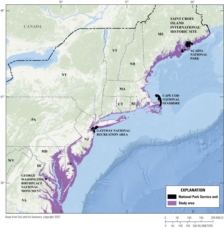
Map showing the location of the coastal change likelihood domain that stretches from Maine to North Carolina and covers the coastal zone between −10 and +10 meters relative to mean high water. The National Park Service units (data from National Park Service, 2022) considered for coastal change likelihood assessment are shown on the map.
2. Methodology
This section describes the methodology and structure of the CCL study, including the source data, processing, and classification. Detailed descriptions of software, source information, spatial analysis tools and code, scale, and accuracy assessment information are provided in the metadata files for geospatial data layers in Sterne and others (2023). The methodology of the CCL assessment is described in this section as step sequences through the decision tree framework for the fabric dataset (section 2.1), the assembly of the hazards datasets (section 2.2), and finally the machine learning methods that create the maximum change likelihood and hazard-type datasets (section 2.3).
2.1. The Coastal Fabric Dataset
2.1.1. Classifying the Fabric Dataset
An ordinal scale (table 3) was established for the coastal fabric dataset, and the scale serves to compare the relative resistance of coastal landscapes. The scale has eleven values, 0 to 10, that indicate the relative resistance, or conversely, responsiveness of a landscape to change based on its geologic and ecologic composition and textures, shear strength, and resilience in response to forcing, much of which is captured in the record of historical change, such as shoreline accretion rate or dune height. A value of 0 indicates a submerged landscape and serves as a “no data” value for this assessment. A value of one indicates that a landscape is extremely likely to resist change, and a value of ten indicates that a landscape is extremely likely to respond by changing in the next decade. This ranking system will later be combined with the hazards to inform a final CCL outcome.
The fabric datasest is managed using the ordinal scale (table 3) and a hierarchical classification framework, or decision tree to synthesize available landscape-specific data to answer the question, “What areas of the coastal landscape are most likely to change on a decadal scale?” The fabric ordinal scale classes generated by stepping through levels in the tree address the likelihood that the landscape will change or resist change given inherent sensitivity of its physical structure, historical observed trends, and empirical information. The decision tree is managed using Esri ArcGIS Pro (ver. 2.6.3; Esri, 2020a) and a Jupyter Notebook (.ipynb) file (Jupyter, 2020) to automate processes using the ArcPy scripting package (Esri, 2020b). Conditional statements were the primary tool used to parse data and apply metrics if certain parameter thresholds were met.
In decision tree models, the root node represents the entire sample or an overarching question (fig. 3). Decision nodes split into further possibilities, and leaf nodes or terminal nodes are an outcome that cannot be further categorized. In this report, the root node is the question “Is the coast landscape likely to change on a decadal scale?” and the question remains the same passing through levels or nodes that refine the answer. In the decision tree used for this assessment, there are three shapes that differentiate between the types of nodes; the root node is encircled at the top of the tree; decision nodes are in rectangles; and leaf nodes (or terminal nodes) are triangles. Subtrees are branches beyond the land cover classes (third decision) and nuance the ordinal scale established by landcover type (table 3; values 0 to 7).
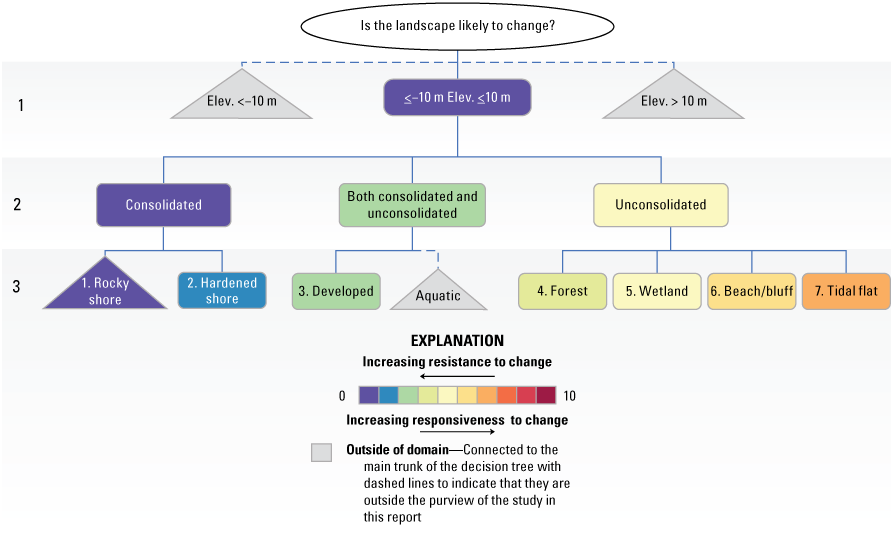
A nonbinary decision tree, through the definition of land cover type (first three levels), for a coastal change likelihood framework. Further levels below the land cover type are presented in figures 4A, 5A, and 7A, 8A, 9A, 10A, 11A, 12A, 13A. Terminal nodes are indicated by triangles; terminal nodes have no data, are shaded in gray, and are connected to the main trunk of the decision tree with dashed lines and are outside the domain of this study. Decision (branching) nodes are indicated with rectangles. Numbers inside nodes indicate the fabric value or the landscape’s resistance to change, where low values are hard or very resistant and high values are soft or less resistant (table 3). The numbers on the left indicate the tier or level of the tree, and the color ramp indicates resistance to change from extremely low (warm colors) to extremely high (cool colors). Elev., elevation; <, less than; >, greater than; m, meter.
Table 3.
Fabric resistance values and definitions for land cover classes in the fabric dataset of the framework for a coastal change likelihood assessment.[Fabric dataset refers to the data related to the resistance or integrity of the coastal landscape. Fabric values greater than 7 are not used for land cover classes but are included here with value definitions to show propensity to change increases associated with landscape specific metrics in the decision tree. Landform examples shown here for values 1-7 are before the addition of landscape-specific metrics. Subtree decisions will affect the final fabric value and thus may not correspond to the landform described here. Shear strength is approximate value and is from Onasch (2010) unless otherwise noted. kPa, thousand pascal; MPa, million pascal; ~, approximately; >, greater than; —, no value]
| Fabric resistance to change | Shear strength | Fabric value | Fabric value explanation | Example landform* |
|---|---|---|---|---|
| No estimate | No estimate | 0 | No fabric value estimate at this time | Aquatic or submerged landscapes |
| Consolidated landscapes; very resistant or nearly incapable of measurable change over decadal-scale steady-state processes | Very high (>3 MPa) | 1 | Extremely resistant | Bedrock cliffs or bluffs; wave cut platforms, and rocky shore shores |
| Consolidated structures built to resist coastal processes. | High (>2 MPa) | 2 | Very resistant | Seawalls, groins, riprap, bulkheads, docks, piers, jetties, and other manmade structures |
| Consolidated and unconsolidated human-modified environments that are resistant, but not built to resist coastal processes; typically, afforded some protection due to setback and elevation | Moderate (>500 kPa) | 3 | Resistant | Developed land classes and impervious surfaces, including developed open space |
| Unconsolidated forested environments that are capable of response; typically afforded some protection due to setback, elevation, and vegetation | Low (~20 to 200 kPa; Osman and Barakbah, 2006) | 4 | Mostly resistant | Forests |
| Unconsolidated wetland environments that are capable of response, afforded some protection to no protection from coastal hazards or processes | Very low (~4 to 30 kPa; Jafari and others, 2019) | 5 | Somewhat resistant to slightly responsive | Marshes and wetlands |
| Unconsolidated bluff and beach environments that are capable of response, afforded some to no protection from coastal processes | No to low (0 to 24 kPa; Boudreaux, 2012) | 6 | Slightly resistant to somewhat responsive | Sand and gravel beaches and bluffs |
| Unconsolidated environments that are capable of response, afforded some to no protection from hazards and frequently submerged or flooded | No to low (0 to 24 kPa; Boudreaux, 2012) | 7 | Somewhat responsive | Mud flats and sand bars |
| An environment (listed above) that has associated measured change data that increases the fabric value | — | 8 | Mostly responsive | Saltmarsh environment with low elevation and high unvegetated-to-vegetated ratio value |
| An environment (listed above) that has associated measured change data that increases the fabric value | — | 9 | Very responsive | Barrier beach with long-term shoreline change and low dunes |
| An environment (listed above) that has associated measured change data that increases the fabric value | — | 10 | Extremely responsive | Not used within the fabric dataset for this pilot study |
2.1.2. Defining the Domain
The answers to the decision tree’s root question are refined by adding datasets that inform the overarching question and applying the ordinal scale in tiers of the tree. The first decision uses elevation data to define the domain for the northeastern United States by selecting the area greater than −10 and less than +10 m MHW (similar to Lentz and others 2015). Areas with an elevation outside this domain are excluded from analysis because they are unlikely to experience decadal-scale coastal landscape-related change. Subsequent tiers in the tree serve to reorganize or mute nodes within the −10 to +10-m domain.
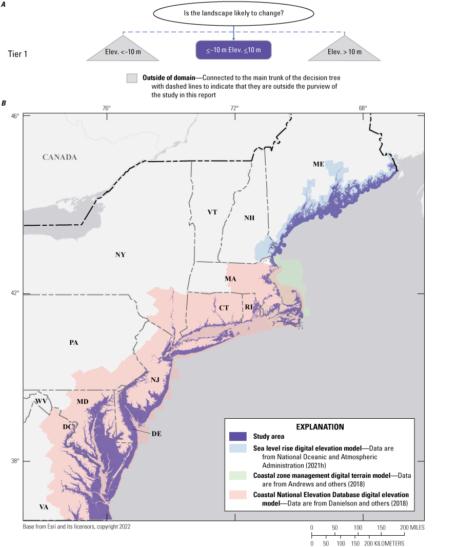
Nonbinary decision tree and map showing the first level of decision for the coastal change likelihood assessment applied to the northeastern United States. A, The first decision node defines the coastal zone or domain of this study using elevations greater than −10 and less than +10 meters relative to the Mean High Water datum. B, A digital elevation model is used to define the area of the coastal zone that is most likely to change as a result of decadal-scale coastal hazards.
Three elevation data sources are used to define the domain (table 4): Coastal National Elevation Database (CONED; Danielson and others, 2018) for Massachusetts through Virginia; a continuous terrain model of Massachusetts (Andrews and others, 2018), which covers Massachusetts; and the National Oceanic and Atmospheric Administration (NOAA) sea level rise data viewer (National Oceanic and Atmospheric Administration, 2021e, h) for the subaerial topography of New Hampshire and Maine. These data were layered such that CONED (1-m resolution) was given priority (Massachusetts through Virginia), and the Massachusetts terrain model (10-m resolution) or the NOAA sea level rise viewer data (3-m topographic resolution) were used to fill in CONED gaps. Elevation data were transformed from their native vertical coordinate systems to a MHW reference using VDatum (version 4.3; National Oceanic and Atmospheric Administration, 2020b). A high-resolution, seamless topographic bathymetry dataset for New Hampshire and Maine does not exist, so the domain in these two States extends seaward (beyond the −10 m isobath) to the edge of the aquatic land cover category as defined by the Coastal Change Analysis Program (C–CAP; National Oceanic and Atmospheric Administration, 2019). The domain extent beyond the shoreline primarily supports the hazard datasets (section 2.2). The submarine landscape is not classified in the fabric dataset but is essential for appending coastal hazards, such as waves, sea level rise, and tidal flooding.
Table 4.
Data sources included in the fabric dataset for a pilot study of a coastal change likelihood assessment.[Fabric dataset refers to the data related to the resistance or integrity of the coastal landscape. m, meter]
| Data type | Source | Resolution | Citation |
|---|---|---|---|
| Elevation1 | Coastal National Elevation Data | 1-m | Danielson and others (2018) |
| Continuous bathymetry and elevation models of the Massachusetts coastal zone and continental shelf | 10-m | Andrews and others (2018) | |
| National Oceanic and Atmospheric Administration coastal inundation digital elevation model | 3-m | National Oceanic and Atmospheric Administration (2021e,h) | |
| VDatum | 10-m | National Oceanic and Atmospheric Administration (2020b) | |
| Land use and land cover | Coastal Change Analysis Program-derived land cover for Maine, New Hampshire, Massachusetts, Rhode Island, Connecticut, New York, Delaware, and Maryland | 10-m | National Oceanic and Atmospheric Administration (2019) |
| Virginia land cover | 1-m | Virginia Geographic Information Network (2020) | |
| New Jersey land cover | Vector polygons | New Jersey Department of Environmental Protection Bureau of GIS (2019) | |
| Chesapeake Bay Project | 1-m | Chesapeake Conservancy (2018) | |
| Shore type | Environmental sensitivity index shoreline type | Vector polylines and polygons | National Oceanic and Atmospheric Administration (2017) |
| Shoreline change | National assessment of shoreline change | Vector transects perpendicular to shore at 50-m interval | Himmelstoss and others (2010) |
| Massachusetts shoreline change | Vector transects perpendicular to shore at 50-m interval | Himmelstoss and others (2018) | |
| Marsh vegetation state | Unvegetated-to-vegetated ratio | 30-m | Couvillion and others (2021) |
| Wetlands | National Wetland Inventory | Vector | U.S. Fish and Wildlife Service (2020) |
| Marsh unit designation | Watershed Boundary Dataset | Vector | Moore and others (2019); U.S. Geological Survey (2020) |
| Dune height | Coastal hazards database | Polyline vector | Doran and others (2020) |
The extents of the elevation source domains are displayed in figure 4B.
2.1.3. Land Cover Data Sources, Classification, and Accuracy
Tiers one and two in the decision tree for the fabric dataset are further refined using land cover raster data and shoreline-type vector data. A total of eight land cover classes are included. Five classes were derived from land cover raster-based data sources (renamed as aquatic [submerged], wetland, unconsolidated shore and bluff, forest, and developed areas [table 4]): the C–CAP high-resolution, 10-meter per pixel (mpp) resolution data (National Oceanic and Atmospheric Administration, 2019), the Chesapeake Conservancy’s 1-m resolution land cover data project layer (Chesapeake Conservancy, 2018), the New Jersey Department of Environmental Protection’s Bureau of GIS land use and land cover shapefile data product (New Jersey Department of Environmental Protection Bureau of GIS, 2019), and the Virginia Geographic Information Network’s 1-m resolution land cover data (Virginia Geographic Information Network, 2020). The three remaining classes (tidal flats, hardened shorelines, and rocky shores) were derived from vector shoreline-type data from polygon and polyline datasets available by coast and by State from NOAA’s environmental sensitivity index (ESI) dataset (National Oceanic and Atmospheric Administration, 2017).
Land cover data accuracy is important to the overall accuracy of CCL, because these are the primary data that form a foundation to which other data sources are appended. The reclassified land cover dataset that was derived from the raster- (C–CAP and others) and vector-based (ESI) source data (table 4) were assessed for accuracy using ArcGIS Pro (version 2.5). Approximately 250 random points were created using a stratified random sampling scheme, where points were randomly distributed within each land cover class, proportional to the relative size of each class. A confusion matrix was generated at the end of the accuracy assessment that characterized the overall accuracy of the land cover classification, as well as the individual sources used to create the classes. The results of the accuracy assessment are described in section 3 of this report.
2.1.4. Defining the Fabric
Taken together, these land cover categorizations capture inherent qualities that reflect landscape integrity or resistance to change. For example, differences among these land cover classifications can be used to determine whether an area is primarily submerged or exposed, consolidated or unconsolidated, and vegetated or unvegetated, all of which are valuable characteristics to consider when assessing if a coast will change. The ordinal scale (table 3) captures these relative differences among landscapes. The resistance (or conversely responsiveness) to change is defined as the composition, material strength, and proximity and elevation relative to coastal and marine-based hazards and processes. Ordinal values compare the erodibility of different land cover classifications or the resistance of a material or soil to erosional processes, using intrinsic properties of the landscape that influence its ability to remain unchanged by common coastal processes. Erodibility of the different land cover types depends on a variety of factors, especially for unconsolidated land covers, and includes characteristics such as texture, cohesion, infiltration, plasticity, organic and clay content, and shear strength (Morgan, 2005).
Based on the resistance of the landscape, the data in the fabric dataset were assigned values from 0 to 10 (table 3). A value of 0 is associated with submerged landscapes, which lack subsequent decisions and data to assign a fabric value; therefore, a fabric value of 0 is equivalent to No Data. Values 1 through 7 are associated with the subaerial landscapes from the land cover and ESI (National Oceanic and Atmospheric Administration, 2017) shoreline-type datasets and are often further nuanced within the landscape subtrees. Values 8 through 10 are values greater than the land cover assigned values because they have decision nodes (tiers; for example, estuarine wetland), which incorporate metrics (for example, mean marsh elevation) to further specify a more nuanced fabric value.
When incorporating this information in the decision tree, the first consideration is whether the data describe an area that is consolidated (rocky and hardened shores), consolidated and unconsolidated (developed and aquatic), or unconsolidated (vegetated forests and marshes, or beaches, bluffs, and tidal flats; fig. 5). The aquatic land cover class—defined as any area submerged throughout the tidal cycle as classified in the 2013–17 source imagery of land cover—is a terminal node, such that there are no other decisions associated with this landscape classification. A lack of consistent, high-resolution, and regionally seamless data sources for seafloor substrate precludes subsequent decisions of the aquatic landscape. Although other land cover classes such as beaches, tidal flats and marshes may experience tidal flooding, they do not remain submerged through the duration of the tidal cycle and are, therefore, not considered aquatic.
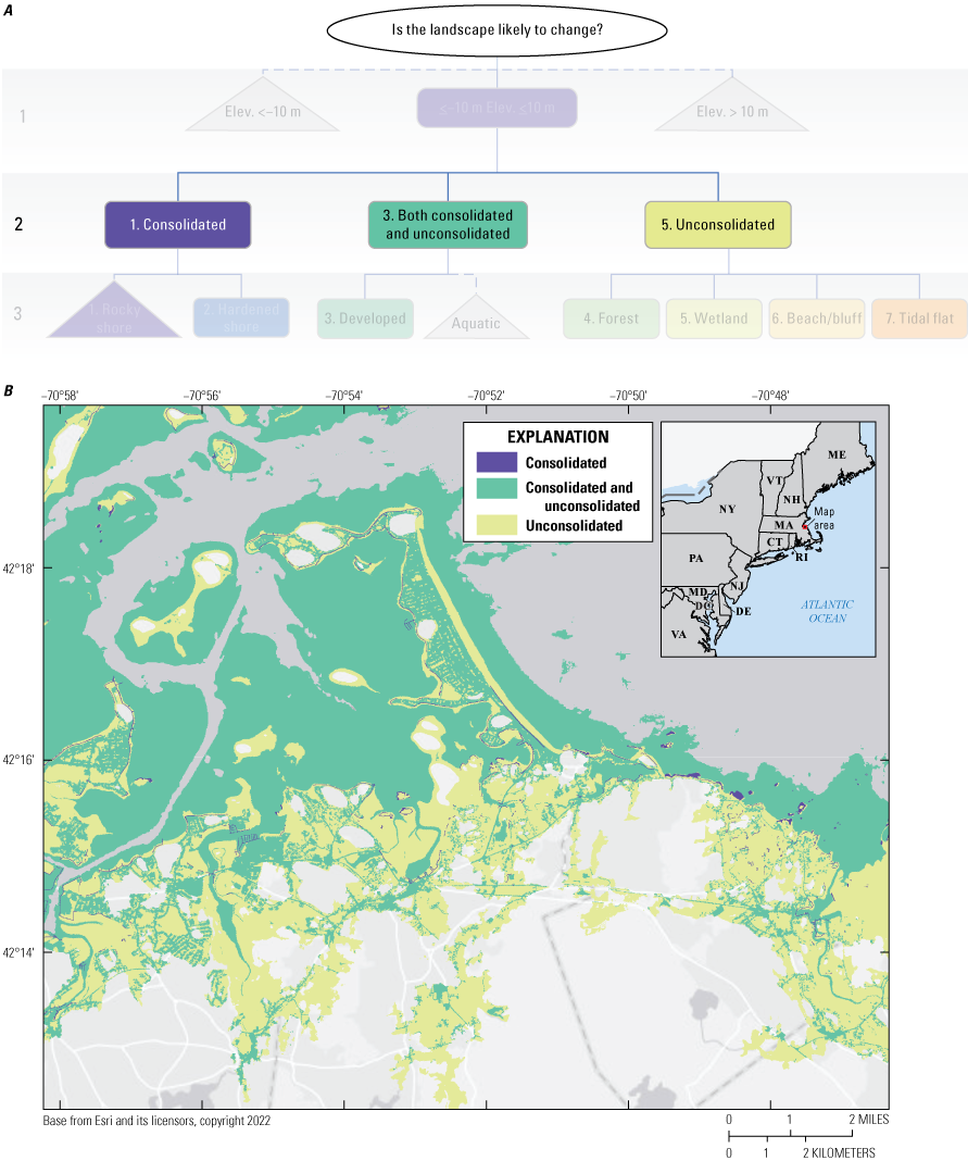
Nonbinary decision tree and map showing the second level in a tree for a coastal change likelihood pilot study for the northeastern United States. A, The second tier of decisions in the decision tree for the fabric dataset differentiates among consolidated, unconsolidated, and a hybrid category (consolidated and unconsolidated) that applies to developed and aquatic land cover types. B, The spatial distribution of consolidated, unconsolidated, and hybrid (consolidated and unconsolidated) land cover classifications.
The third tier of the decision tree (fig. 3) considers the land cover type and assigns a likelihood based on the fabric scale (table 3) and the type of land cover (fig. 6). This initial ordering of eight common coastal landscapes is the first step in creating the fabric value and eventually, change likelihood outcomes. Subsequent divisions associate land cover-specific information to further discretize resistance within the decision tree.
Map showing the land cover classes used in the decision tree for the fabric dataset for a coastal change likelihood pilot study for the northeastern United States. The values preceding the name of the land cover class are defined in table 3.
2.1.5. Subtree Data Sources, Derivatives, and Processing
Following the eight class land cover distinctions (fig. 6) made in the third tier of the decision tree, land cover specific branches were added for classes where datasets exist that could further elucidate the fabric’s resistance to change. As noted earlier, all land cover classes except for aquatic and rocky shore have subsequent change likelihood decisions that further delineate the landscape.
Elevation, slope, and wetland elevation within a hydrologic boundary (described later in this section) are incorporated in the decision tree as landscape-specific datasets for forests, developed areas, and wetlands. The role of elevation (Danielson and others, 2018; Andrews and others, 2018; National Oceanic and Atmospheric Administration, 2021h) in the domain definition of this study is described in section 2.1.2. To calculate slope from the composite elevation grid, a pixel-to-pixel-based slope calculation was executed in ArcGIS Pro version 2.5 using degree of slope as the unit output. A 6-degree slope was chosen as a threshold between low and high slopes for forested and developed landscapes by mapping slope by contours and charting slope distributions across the domain.
Shoreline change metrics are decision nodes for unconsolidated and hardened shorelines, wherever available. Data sources for shoreline change rates include the national assessment of shoreline change (Himmelstoss and others, 2010) and the Massachusetts shoreline change project (Himmelstoss and others, 2018); these projects include long-term (78 or more years) and short-term (about 30 years) shoreline change rates for sandy, open ocean coasts between Maine and Virginia. The Massachusetts shoreline change project also includes rates of change for some back barrier and wetland shorelines. Shoreline change rates are based on vector transects that are perpendicular to the shoreline at 50-m intervals. Transects were gridded at 10-m resolution, and gaps between adjacent 50-m spaced transects were interpolated. The regression rate associated with each long-term transect was then compared to the reported 90th percentile confidence interval of the data. Areas that overlapped transects with a higher reported regression rate than uncertainty, capturing a high degree of confidence of shoreline change at the location, were assigned an increase in fabric value. Otherwise, low-confidence transects (magnitude less than the 90th percentile confidence interval) did not influence the fabric value and produced the same outcome as no data, capturing the high degree of uncertainty in the shoreline change rate at these locations.
Dune height data were extracted from the national assessment of hurricane-induced coastal erosion hazards (Doran and others, 2020) and were applied to unconsolidated and hardened shore classes, wherever dune height data are present. Dune heights were appended to the shoreline change transects and gridded at the same resolution as shoreline change metrics. Thresholds for high- and low-elevation dunes are set at greater than (>) 3 m and less than or equal to (≤) 3 m, respectively, to identify a threshold between areas that have less protection from overwash or overtopping during storm events and areas that are likely more protected from overwash (Sallenger, 2000).
The data sources for decisions on the subtree related to the wetland land cover class included elevation (Andrews and others, 2018; Danielson and others, 2018; National Oceanic and Atmospheric Administration, 2021h) relative to mean hydrologic unit elevation (U.S. Geological Survey, 2020), palustrine, estuarine, and marine designations from the National Wetland Inventory (NWI; U.S. Fish and Wildlife Service, 2020), and unvegetated-to-vegetated ratios (UVVRs; Couvillion and others, 2021; Ganju and others, 2022). NWI polygons were used to parse wetlands into either palustrine wetlands or estuarine and marine wetlands. Estuarine and marine wetlands were further grouped by 12-digit hydrologic unit code (HUC12; U.S. Geological Survey, 2020) with a mean elevation determined for the hydrologic unit. The hydrologic units were used to approximate conceptual marsh units (Defne and others, 2020) and compare pixel-level elevation to mean salt marsh elevation derived within each HUC12 hydrologic unit. Pixels with elevation below the mean hydrologic unit elevation were considered low elevations, and pixels with elevation above the mean hydrologic unit elevation were considered high elevations. Finally, satellite-derived UVVR metrics at their source 30-m resolution were used to further categorize estuarine and marine wetlands (Couvillion and others, 2021).
2.1.6. Subtree Scaling
Subtree branching beyond the land cover designation tier of the fabric decision tree (tier 3; fig. 6) occurs by adding land cover-specific data sources, described by land cover type in the following sections. The relative fabric value estimate is adjusted for each node in the subtrees. For example, as elevation and slope data are added to a given forest or developed pixel in the fabric decision tree, the fabric value for the node that parses the numerical (or in some cases categorical) data will be adjusted up or down the ordinal scale (table 3). Subtree figures associated with land cover type in sections 2.1.6.1 through 2.1.6.7 illustrate how this adjustment works and the relative increase or decrease in fabric value as data and metrics are filtered through the decision tree based on a landscape’s intrinsic properties and resistance to change. Appendix 1 displays the fabric tree for Gateway National Recreation Area, which was selected as a test case in the pilot study.
2.1.6.1. Rocky Shore Landscapes
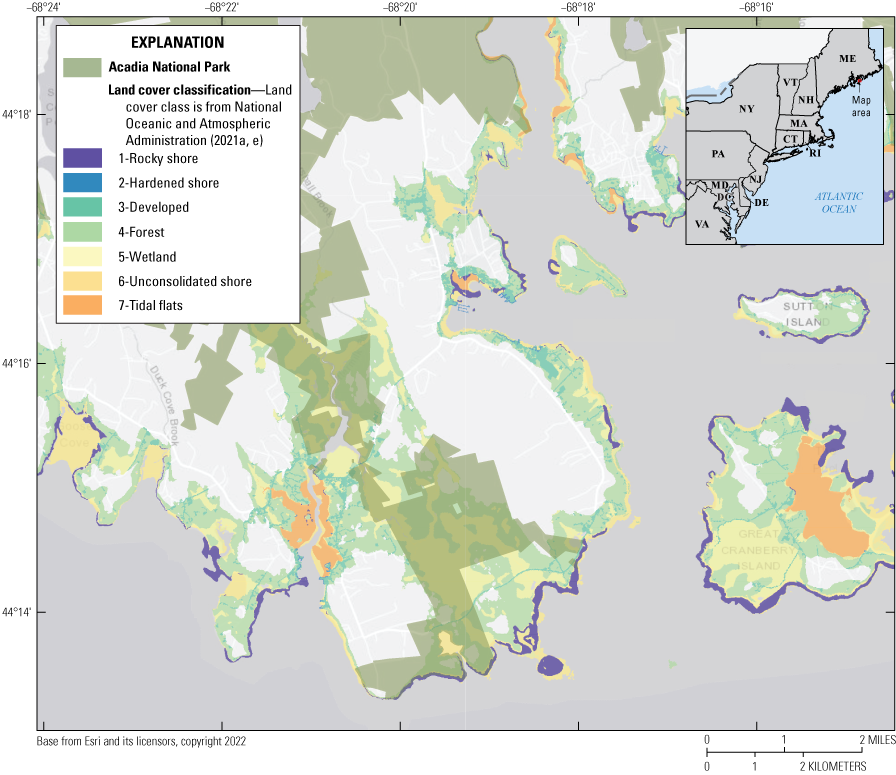
Rocky shore land cover classes have high shear strength (table 3) and are not likely to change on a decadal scale. Rocky shore landscapes are a terminal node in the decision tree (fig. 7A) and are assigned the lowest fabric value of 1 (fig. 7B), or extremely resistant to change due to their high shear strength. The elevation of a rocky shore coast with regard to sea level rise will be considered in the hazards dataset described in section 2.3, which can influence the final CCL value for low-lying rocky shores.
Nonbinary decision tree and map showing the rocky shore land cover classification in a coastal change likelihood pilot study for the northeastern United States. A, Rocky shore landscapes are a terminal node in the decision tree and have a fabric value of 1, which indicates that they are extremely resistant to coastal change. B, Rocky shores with a fabric value of 1 along the Maine coastline in Acadia National Park. Fabric refers to the resistance or integrity of the coastal landscape.
2.1.6.2. Hardened Shore Landscapes
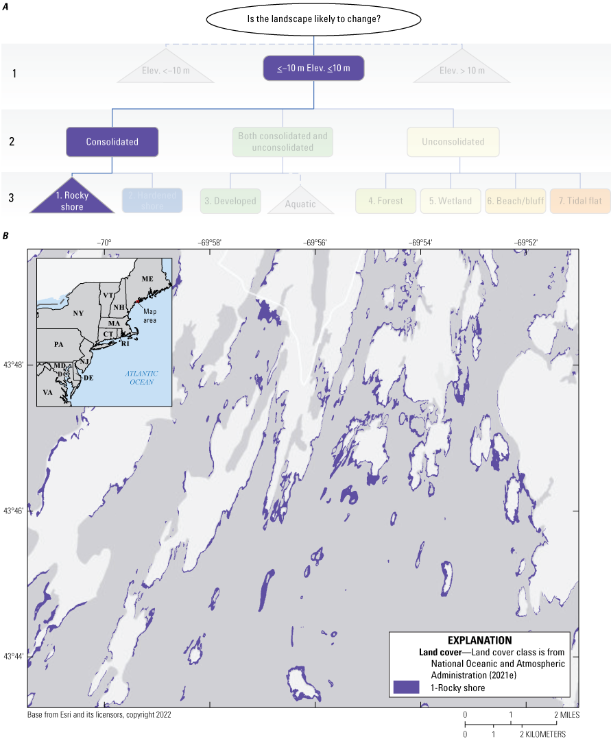
Similar to rocky shores, hardened shores also have a relatively high shear strength (table 3) thus a low likelihood of decadal-scale change. Engineered structures or hardened shorelines are often placed to minimize coastal change and hold the position of the land-water interface; however, they are inherently less resistant than bedrock shores. Shoreline change can undermine the stability of some structures, especially those along the open ocean, rendering them unstable where erosion is present or obsolete in areas of high net accretion. Likewise, dune height metrics (Doran and others, 2020) can capture low elevations commonly adjacent to seawalls and other open-ocean shore protection that can reflect an absence of natural features to buffer hazards (that is, storm) effects.
To identify where shoreline change and dune heights may affect the future integrity of hardened structures, a decision is added that reflects the availability, magnitude, and confidence of coincident USGS shoreline change data (Himmelstoss and others, 2010, 2018) and dune height metrics (Doran and others, 2020). The subtree for hardened shorelines is highlighted in figure 8A with fabric scale values of 2 to 4 for terminal nodes (fig. 8B); values of 2 indicate adjacent shoreline change or dune height information is low confidence or unavailable, values of 3 indicate adjacent high confidence shoreline change rates or low dune height, and a value of 4 indicates the presence of both high-confidence shoreline change and low dune height. As with other nodes in the tree, these values are intended to capture the inherent resistance of these features to change before the introduction of hazard-specific data (see section 3).
Nonbinary decision tree and map showing the hardened shore land cover classification in a coastal change likelihood pilot study for the northeastern United States. SCC, shoreline change confidence; DH, dune height. A, The decision tree for hardened shores has two branches: shoreline change or dune height information that is either of low confidence or unavailable (value 2) or high confidence shoreline change rates or low dune height (value 3) B, Hardened shoreline distributions along the Atlantic Ocean, adjacent to Gateway National Recreation Area in New Jersey and New York.
2.1.6.3. Developed Landscapes
Developed areas, especially those with consolidated substrate are unable to change or adapt to coastal hazards and processes without human intervention. Elevation is often considered the most important indicator of inundation or flood risk in developed areas (Gesch, 2009; National Oceanic and Atmospheric Administration, 2021h). Areas with low or no slope are also considered more vulnerable to coastal inundation (National Research Council, 2007). Elevation metrics are the key factors to assigning change likelihood for developed areas at a decadal scale because these developed areas are at an increased risk of experiencing short or long-term flooding.
To refine the fabric value determination for developed areas, four branches were created in the decision tree to reflect the significance of elevation (threshold of 2 m) and slope (threshold of 6 percent) using the same source data used in the domain determination in the root node. Developed areas with low elevation (less than [<] 2 m) and gentle slopes (less than 6 percent) are less resistant to change in the coming decade (fabric value of 5), whereas developed areas with high elevation (>2 m) and steep slopes (greater than 6 percent) are more resistant to change (fabric value of 3), due to protection afforded by setback and elevation. Combinations of high elevation and low slope or low elevation and high slope were given a fabric value of 4, or more resistant than responsive. Figure 9A shows the subtree, with ordinal scale values for terminal nodes with values between three and five, which is the fabric value based on intrinsic landscape properties (fig. 9B) before the introduction of hazard-specific data (see section 3).
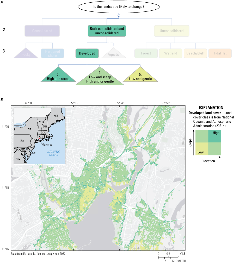
Nonbinary decision tree and map showing the developed land cover classification in a coastal change likelihood pilot study for the northeastern United States. A, Developed landscapes have three branches in the decision tree. Areas with high elevation (greater than 2-meters [m]) and steep slopes (greater than 6 percent) have a fabric value of 3. Areas with high elevation and gentle slopes (6 percent of less) or low elevation (less than or equal to 2-m) and steep slopes have a fabric value of 4. Areas with low elevation and low slopes have a fabric value of 5. B, Developed landscapes with varying slopes and elevations are mapped out according to the subtree for the developed land cover classification (fig. 9A) for an urban area of Connecticut.
2.1.6.4. Forested Landscapes
Forests at or near sea level are susceptible to die off due to sea level rise, land subsidence, and storm surge events. Ghost forests are areas of dead trees commonly found within low-lying coastal areas that occur due to saltwater intrusion into freshwater aquifers (Kirwan and Gedan, 2019). As in developed areas, forest elevation is a key factor in determining whether a forest will persist or remain unchanged in the next decade. Low relative slope can be an advantage or disadvantage in forested landscapes. For example, forests at the edge of coastal bluffs and banks are more likely to slump or slide. However, marsh migration may be more likely at low slopes.
For the purposes of this study, steep forest slopes are considered less resistant compared with steep slope developed areas. This distinction is made to account for the possibility of slope failure along forested coastal banks, which is more likely to occur over decadal timescales when compared to marsh migration. The same thresholds are used for elevation and slope for forests as in developed landscapes. However, an inverse relationship between slope and elevation was applied, where gentler slopes in forested areas were considered a lower fabric value than steep slope forested areas. Forests with low elevation (<2 m) and steep slopes (>6 percent) were assigned a fabric value of 6, whereas forests with high elevation (>2 m) and low slopes (<6 percent) were assigned a fabric value of 3. Combinations of high elevation and high slope or low elevation and low slope were given fabric values of 4, and 5, respectively. The subtree for forested landscapes is shown in figure 10A, and the mapped distribution of fabric values for terminal nodes through the subtree is shown in figure 10B.
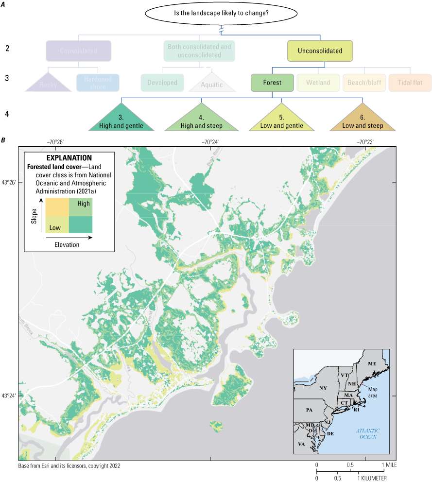
Nonbinary decision tree and map showing the forested land cover classification in a coastal change likelihood pilot study for the northeastern United States. A, Forested landscapes have four terminal nodes below land cover in the decision tree. Areas with high elevation (greater than 2-meters [m]) and gentle slopes (less than or equal to 6 percent) have a fabric value of 3. Areas with high elevation and steep slopes (greater than 6 percent) have a fabric value of 4. Low elevation (less than or equal to 2-m) and low slopes have a fabric value of 5. Areas with low elevation and steep slopes, which are more prone to slope failure, have a fabric value of 6. B, Forested landscapes with varying slopes and elevations are mapped out according to the subtree for the forested land cover classification (fig. 10A) for a forested coastal area in Maine.
2.1.6.5. Wetland Landscapes
Wetland or marsh landscapes are often initially classified according to whether they are fresh water (palustrine) or saltwater (marine and estuarine). The first step in assessing marsh landscapes included parsing all marsh pixels according to palustrine or marine and estuarine type using data from the NWI (U.S. Fish and Wildlife Service, 2020). Data reflecting saltwater intrusion into groundwater systems were not incorporated but could be an important addition to better refine palustrine systems in the future. For marine and estuarine wetlands, UVVR (Couvillion and others, 2021; Ganju and others, 2022) metrics were applied along with a mean marsh elevation (relative to mean sea level) calculated by the HUC12 hydrologic unit designation of the hydrologic basin (Moore and others, 2019; U.S. Geological Survey, 2020).
The UVVR is derived from Landsat imagery and can be used to evaluate the health of coastal wetlands (Ganju and others, 2022). Following the determination of the type of wetland (palustrine or estuarine and marine), the wetlands were sorted based on pixel elevation relative to the mean marsh elevation within the hydrologic unit. Pixel elevations below mean marsh elevation are more likely to change than pixels above mean marsh elevation, which is shown as mean sea level (fig. 11). According to Ganju and others (2020, 2022), the most resilient marshes have a UVVR less than 0.15 and high elevation relative to mean marsh unit elevation. By contrast, the marshes most susceptible to coastal change have low relative elevation and UVVR values greater than 0.4 (Ganju and others, 2017a, b) and are likely to transition to an open water or tidal flat landscape in the coming decade.
Areas with low elevation and low UVVR (<0.15), high elevation and moderate UVVR (0.15 to 0.4), and all marsh areas outside NWI marine and estuarine salt marshes were assigned a value of 5. Those with high elevation and high UVVR (greater than 0.4) were given a value of 6. Low elevation pixels with moderate UVVR (>0.15 and <0.4), were given a fabric value of 7. Estuarine wetlands, which tend to be more protected from open water conditions, were ranked with slightly higher fabric values: those with lower than mean marsh elevation and moderate UVVR (0.15 to and 0.4) were given a fabric value of 7, whereas those with higher than mean marsh elevation and high UVVR (>0.4) values were given a fabric value of 6. The subtree that shows fabric values for wetland landscapes is shown in figure 11A, and the mapped distribution of fabric values for terminal nodes through the wetland subtree is shown in figure 11B.
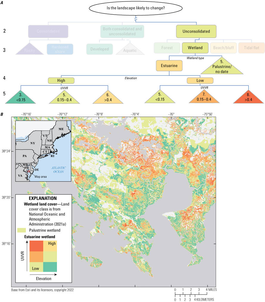
Nonbinary decision tree and map showing the wetland land cover classification in a coastal change likelihood pilot study for the northeastern United States. A, Wetland landscapes have seven terminal nodes through three branches in the subtree for the wetland land cover classification. Palustrine areas have a fabric value of 5. Areas with high elevation (above mean marsh elevation) and low (less than 0.15), moderate (0.15 to 0.4), or high (greater than 0.4) unvegetated-to-vegetated ratio (UVVR) values, have fabric values of 3, 5, and 6, respectively. Low elevation (below mean marsh elevation) and low, moderate, or high UVVR values have fabric values of 5, 7, and 8, respectively. B, Wetland landscapes with varying salinity, elevation, and UVVR metrics are mapped out according to the wetland subtree (fig. 11B) for a wetland area along the eastern shore of the Chesapeake Bay. <, less than; >, greater than.
2.1.6.6. Unconsolidated Landscapes
Shoreline change measurements and dune height metrics were used to determine change likelihood for unconsolidated shores (that is, beaches and bluffs) in the decision tree. Long-term shoreline change rates derived from historical shoreline positions were used to highlight dynamic areas of the unconsolidated coastline. Dune height metrics from Doran and others (2020) also exist for many open ocean locations where shoreline change data are present. Unconsolidated shores with no shoreline change data maintain a fabric value of 6, because there is no additional information to refine the estimate. Areas with high shoreline change confidence and high dunes were given a value of 7, and those with low elevation dunes and high shoreline change confidence were given a value of 8. The subtree that shows relative change likelihood for unconsolidated beaches and bluffs is shown in figure 12A, and the mapped distribution of fabric values for terminal nodes through the shore and bluff subtree is shown in figure 12B.
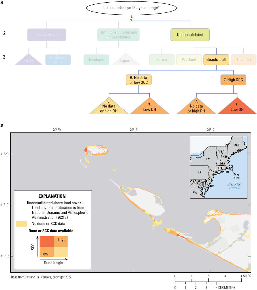
Nonbinary decision tree and map showing the unconsolidated land cover classification in a coastal change likelihood pilot study for the northeastern United States. SCC, shoreline change confidence; DH, dune height. A, Unconsolidated landscapes have three terminal nodes through two branches in the subtree for the bluff and beach land cover classification. Areas that lack shoreline change data or have a low confidence associated with change have a fabric value of 6; areas with high shoreline change confidence and high dunes or no dune height data have a fabric value of 7; and areas with high shoreline change confidence and low dune height elevations have a fabric value of 8. B, Unconsolidated landscapes with varying shoreline change confidence and dune height metrics are mapped out according to the beach and bluff subtree (fig. 12B) for the western end of Nantucket Island, Massachusetts.
2.1.6.7. Tidal Flat Landscapes
Tidal flats are treated similarly to unconsolidated shore in the decision tree, where shoreline change rates and dune heights are indicators of increased or decreased fabric value. For example, a washover-prone section of a barrier island will have tidal flats that are more likely to experience change than sheltered tidal flats protected by high elevation dunes. Tidal flats with no shoreline change data or low confidence data maintained the baseline fabric value of 7, whereas tidal flats with high shoreline change certainty or low dunes had a fabric value of 8. Tidal flats with low elevation dunes and high shoreline change certainty had a fabric value of 9. The subtree that shows fabric values for tidal flats is shown in figure 13A, and the mapped distribution of fabric values for terminal nodes through the tidal flat subtree is shown in figure 13B.
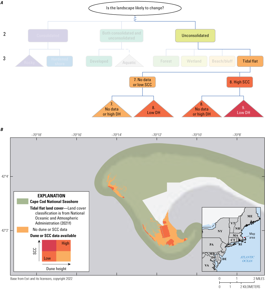
Nonbinary decision tree and map showing the tidal flats land cover classification in a coastal change likelihood pilot study for the northeastern United States. SCC, shoreline change confidence; DH, dune height. A, Tidal flat landscapes have three terminal nodes through two branches of the subtree for the tidal flats land cover classification. Areas that lack shoreline change data or have a low confidence associated with shoreline change have a fabric value of 7, areas with high shoreline change confidence and high dunes or no dune height data have a fabric value of 8; and areas with high shoreline change confidence and low dune height elevations have a fabric value of 9. B, Tidal flat landscapes with varying shoreline change confidence and dune height metrics are mapped out according to the tidal flat subtree (fig. 13A) for part of Cape Cod National Seashore in Massachusetts.
2.2. The Coastal Hazards Dataset
Once the integrity of the fabric is assessed, the next consideration is the hazards that can act on the landscape (fabric). Hazards are often also referred to as exposure (Glick and others, 2011) or as the climatic changes and events that influence the system (fabric). Coastal hazards can occur over a variety of spatial scales, from regional, over hundreds of kilometers (for example, relative sea level rise), to local, across a kilometer or less (for example, storm-driven waves); temporal scales, from ongoing and ever-present to event-driven or acute occurrences; and across all landscapes, with varying effects depending on the ecology, geology, and development of the area. Because of the interdependency of hazards, the landscape, and the spatial and temporal significance of their occurrence, a hierarchical hazard (decision tree) does not provide the same utility as it does for the fabric, but it provides a starting place for managing the hazard data layers and subsequently combining those hazard data with the fabric in the supervised machine learning step of this study (section 2.3).
2.2.1. Managing the Hazards Datasets
This section describes and illustrates the process steps, parameter thresholds, management, and data sources for the hazards dataset. Four questions guide the construction of the hazards datasets:
-
Is this hazard likely to affect the coastal landscape in the near (decadal) term?
-
Is the hazard a perpetual (ongoing, ever-present) or event-driven occurrence?
-
Is this hazard present at this location?
-
What is the magnitude of the hazard?
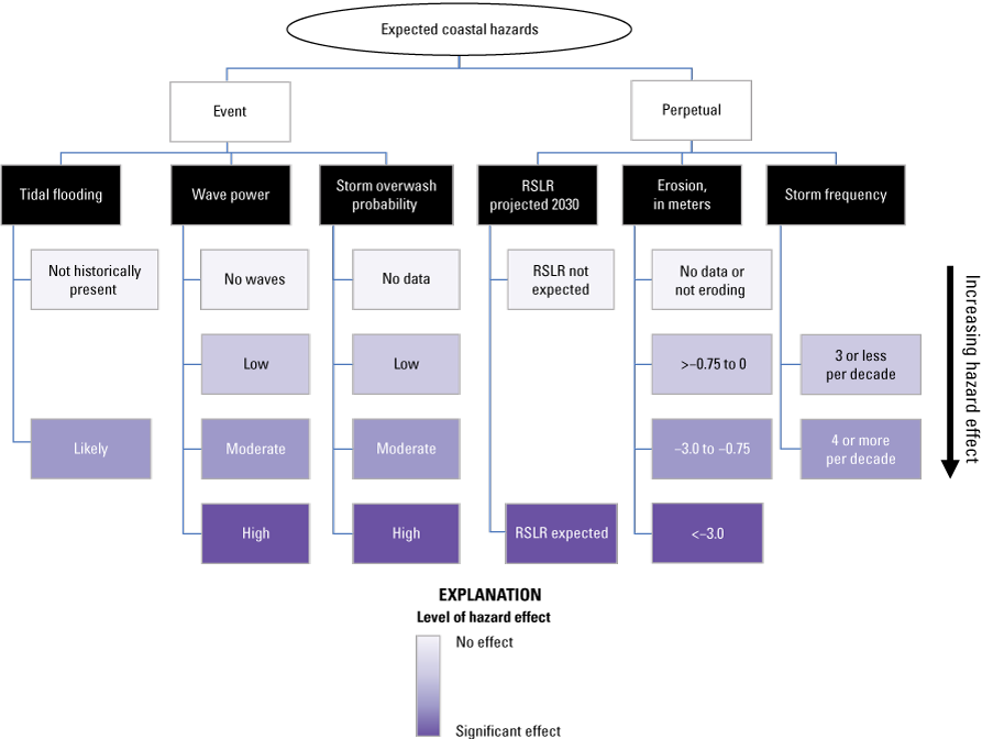
Decision tree showing common coastal hazards evaluated in a coastal change likelihood pilot study for the northeastern United States. Each hazard is broken out into categories based on presence, absence, and magnitude, if relevant. Not all hazards exist across all landscapes. RSLR, relative sea level rise; >, greater than; <, less than.
Table 5.
Common coastal hazard datasets included in a coastal change likelihood pilot study for the northeastern United States.[The hazards datasets are from Sterne and others (2023). The values associated with each threshold are assigned independent of the land cover in this table. Integration of landscape and hazard sources is described in section 2.2.2 of this report. Fabric dataset refers to the data related to the resistance or integrity of the coastal landscape. m, meter; W/m, watt per minute; m/yr, meter per year; >, greater than; <, less than; ≥, greater than or equal to]
| Hazard | Resolution | Source | Values and thresholds |
|---|---|---|---|
| Event hazards | |||
| High tide flooding | About 5 m | National Oceanic and Atmospheric Administration (2020a) | 0; not historically present 1; likely |
| Climatological wave power | Finite element grid | Aretxabaleta and others (2022) | 0; No data or 0 W/m; no wave power 1; >0 to 50 W/m; low wave power 2; >50 to 185 W/m; moderate wave power 3; >185 W/m; high wave power |
| Storm overwash probability | Vector | Doran and others (2020) | 0; no data 1; >0 to 25 percent; low probability of overwash 2; >25 to 75 percent; moderate probability of overwash 3; >75 percent; high probability of overwash |
| Perpetual hazards | |||
| Projected relative sea level rise1 for 2030 | 10 m | Sweet and others (2017) and digital elevation model from the fabric dataset (table 3) | 0; sea level rise flooding not expected by 2030 1; sea level rise flooding expected by 2030 |
| Short-term shoreline erosion rate | Vector transects at 50-m interval gridded to 10 m | Himmelstoss and others (2010, 2018) | 0; no data or not eroding 1; >−0.75 to 0 m/yr; low erosion 2; −3.0 to −0.75 m/yr; moderate erosion 3; <−3.0 m/yr; high erosion |
| Storm recurrence interval | Vector transects gridded to 10 m | Knapp and others (2010) | 0; three or fewer storms per decade; low frequency 1; four or more storms per decade; moderate frequency |
The projected relative sea level rise scenarios from Sweet and others (2017) are vector data with point locations at 1-degree spacing and tidal gage locations. These projections (in centimeters) were added to the Mean High Water datum elevation domain created in the fabric dataset to obtain a 10-m relative sea level rise extent.
2.2.2. A Baseline for Estimating Hazard Effects
Similar to the fabric dataset, an ordinal scale was established for the six hazards used in this study (table 5). The scale serves to display and compare the relative impact of a hazard based on its presence or absence and magnitude, if applicable. The hazards scale has four values, 0 to 3, that indicate the relative significance of the hazard and its magnitude, when applicable, in affecting coastal change across a generic landscape, independent of the fabric. A value of 0 indicates that the hazard is absent. A value of 1 indicates that the hazard is present and that its presence may have a low effect on a generic landscape in the near term, for example, a low erosion rate or low wave power. A value of 2 suggests the presence of a hazard with moderate potential to affect the landscape, for example, moderate erosion rates, likely area of repeat tidal flooding (for example, king tides), or moderate wave power. A value of 3 suggests the presence of a hazard with a high potential to affect the landscape, such as an area of projected sea level rise flooding, high erosion rates, or high wave energy. This ranking of hazard effects establishes additional coastal change drivers beyond those assigned in the fabric dataset (table 3).
2.2.3. The Event Hazard Dataset
Some events or punctuated hazard data, such as tidal flooding, can be classified simply by presence or absence; for example, areas likely to experience high tide (also known as recurrent or nuisance) flooding are solely based on elevation and historical records: either the area becomes submerged during flooding events or it does not. Other event hazard data, such as wave power and storm overwash probability, include discrete thresholds to differentiate between their impact. Thresholds were mined from peer-reviewed literature or established using data ranges (for example, standard deviations and equal interval binning).
To affiliate the geospatial data with the different hazards and magnitudes, unique values are assigned to each hazard using the placement of the single, tens, and hundreds digits, such that the place of the single digit is occupied by high tide flooding, the place of the tens is occupied by wave power, and the place of the hundreds is occupied by storm overwash probability and a magnitude value; for example, a value of 321 is associated with a pixel that lies within a zone characterized by a 75 to 100 percent overwash probability for a category 2 storm (the “3” in the hundred digit place), a moderate wave energy (the “2” in the teens digit place), and presence of historical high tide flooding (the “1” in the single digit place). Each event hazard has between two and four classes associated with its presence, absence, thresholds, or magnitude (fig. 14; table 5). Details about the source data and processing for each hazard layer are described in the remainder of this section and in table 5. Individual event hazards layers were combined into a single georeferenced tagged image format (GeoTIFF) image file by adding the values of the individual grids together. The resultant grid has values between 10 and 341, representing the combination of hazards and their magnitudes that exist for a given area. A complete list of event hazard values and their definitions can be found in the metadata of Sterne and others (2023).
2.2.3.1. Tidal Flooding Data
The tidal flooding layer is based on historical high tide flood events and is derived from NOAA’s flood frequency geospatial data layer (National Oceanic and Atmospheric Administration, 2020a). The original approximately 2.7-m resolution product was resampled to 10 mpp. The tidal flooding layer has two values reflecting the absence or presence of flooding: 1 where historical high tide flooding has been recorded, and thus likely to occur again, and 0 where no recorded flooding has occurred (fig. 15; table 5). Approximately 93 percent of the assessment domain is outside the zone of historical high tide flooding, with the remaining 7 percent within the historical flood zone.
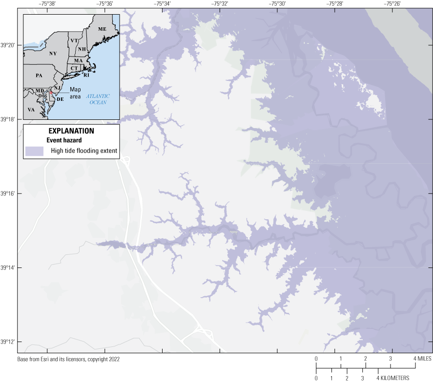
Map showing historic tidal flooding (National Oceanic and Atmospheric Administration, 2020a) for the area in coastal Delaware.
2.2.3.2. Climatological Wave Power Data
Wave power is the energy (per unit length) generated by waves in watts per meter. Aretxabaleta and others (2022) provided a climatological wave power solution, using a coupled ocean-wave model (ADCIRC) over an unstructured (that is, nonrectilinear) grid covering the eastern coast of the United States. For the pilot study in this report, wave power data from Aretxabaleta and others (2022) was rectilinearly gridded at 10-mpp resolution using the finite element grid converted to points. The wave power was interpolated to the extent of the high tide flooding surface to approximate the maximum extent of wave power across a maximum flooding surface so that areas that are likely to experience the greatest wave energy during wave events, storm events, and flooding events can be highlighted.
Wave power thresholds were divided into four classes to discretize wave powers relevant to protected, semiprotected, and unprotected coasts. Data with 0 watt per meter (W/m) or no data indicate no wave power; >0 to 50 W/m indicate low wave power, corresponding to critical wave power threshold for bed erosion used by Mariotti and others (2010) along the Virginia Coastal Reserve; >50 W/m or a significant wave height of 0.2-m to 185 W/m indicate moderate wave power and approximate a threshold between protected and semiprotected coastal settings; and >185 W/m or a significant wave height greater than 0.4 m (Aretxabaleta and others, 2022) indicate high wave power, which is a low threshold estimate based on the source data for open ocean coast wave climates in the Northeast (fig. 16). Just under 5 percent of the subaerial assessment domain is within the wave power zone, with about 0.1 percent of the domain in moderate and high wave power zone; the remaining 95 percent of the subaerial domain is outside the zone likely to be affected by waves.
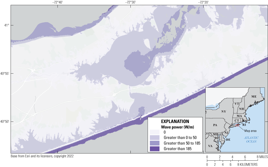
Map showing climatological wave power (energy per unit length) from wind-generated waves (Aretxabaleta, and others, 2022) along the eastern end of Long Island, New York. The areas highlighted are those within the climatological wave power domain that are expected to experience wave energy during wave events.
2.2.3.3. Storm Overwash Probability Predictions
Storm overwash probability is based on storm impact, beach morphology, and hydrodynamic models (Sallenger, 2000; Stockdon and others, 2012). Storm overwash probabilities for an overwash regime during a category 2 storm were derived from Doran and others (2020). A category 2 storm was chosen for this study to represent an intensity level of a tropical or winter storm likely to occur within the study area during the next one to five decades (National Oceanic and Atmospheric Administration, 2018). A spatial join in ArcGIS was used to append overwash probability values (0 to 100 percent) to the shoreline change transects from Himmelstoss and others (2010, 2018) that were used in the fabric dataset. Overwash probabilities were gridded at 10-mpp, and gaps between 50-m transects were interpolated. Storm overwash predictions exist along sandy open ocean coasts where beaches serve as the first line of defense against intense coastal storms (fig. 17). As such, overwash predictions exist for less than 1 percent of the assessment domain, and 0.3 percent of the study area is in the high overwash likelihood range (75 to 100 percent for a category 2 storm).
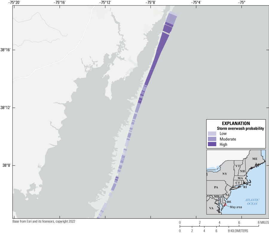
Map showing storm overwash probabilities for a category 2 storm for the eastern shore of Maryland as modeled by Doran and others (2020); the overwash probabilities are mainly in areas along sandy open ocean coasts where storm overwash occurrence during a generic category 2 storm is high (greater than [>] 75 percent), moderate (>25–75 percent), and low (>0–25 percent).
2.2.4. The Perpetual Hazard Datasets
Some perpetual or ongoing hazard datasets like relative sea level rise projections can be classified simply by presence or absence; for example, areas likely to experience sea level rise are based on elevation and sea level rise scenario projections, so either it becomes submerged, or it does not (Sweet and others, 2017). Other hazard data, such as shoreline erosion rates and storm recurrence interval, include discrete thresholds to differentiate between intensity levels. Thresholds were mined from peer-reviewed literature or established using data ranges (for example, standard deviations and equal interval binning). Each perpetual hazard has a unique integer value for data management that represents the presence/absence of the hazards and its magnitude, if applicable, such that the ones place is occupied by relative sea level rise, the tens place is occupied by storm frequency, and the hundreds place is occupied by shoreline erosion rate, and a magnitude value; for example, a value of 311 is associated with a high erosion rate, a low tropical storm recurrence interval, and expected sea level rise by 2020. Each event hazard has between 2 and 4 classes associated with its presence, absence, thresholds, or magnitude, and details about the source data for each perpetual hazard layer are described below and in table 5.
2.2.4.1. Relative Sea level Rise Projections
Relative sea level rise projections were derived from estimates in Sweet and others (2017) for 2030 (global mean sea level of 1-m rise by 2100, intermediate projection). Estimated sea level rise for this scenario was added to the MHW elevation mosaic (same as the domain grid; Danielson and others, 2018; Andrews and others, 2018; National Oceanic and Atmospheric Administration, 2021h) using the Raster Calculator tool. The root mean square error of the CONED elevation dataset is 15 centimeters (cm), and sea level rise projections were made with a low-elevation bias to maximize the extent of the sea level rise flooding surface. This layer was therefore reclassified to a value of 1 for pixels equal to or less than 0.15 m MHW, and 0 for values greater than 0.15 m MHW (fig. 18). Just over 87 percent of the subaerial assessment domain is not expected to be affected by or experience relative sea level rise by 2030, with only the remaining 12 percent likely to experience some effect. Due to the relatively high uncertainty in the elevation data (0.15 to 0.5 cm) and the comparatively low 2030 relative sea level rise estimates (0.12 to 43 cm), this dataset is considered an uncertain estimate of the extent of the effects of sea level rise (Gesch, 2012).
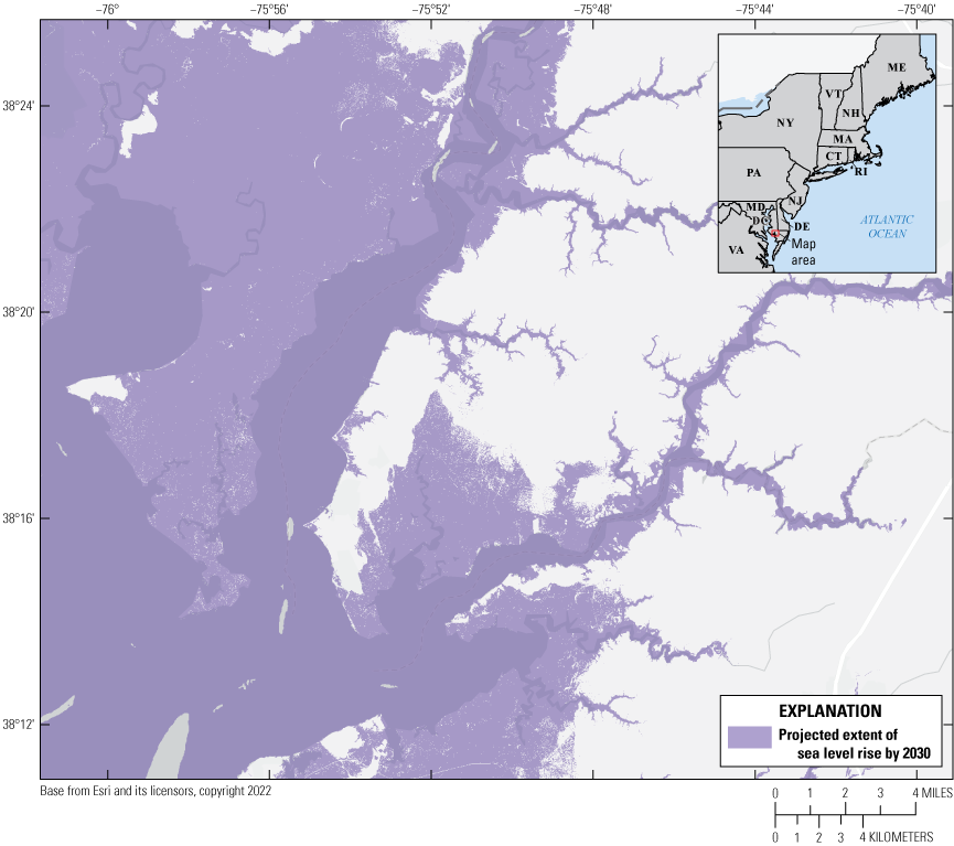
Map showing relative sea level rise projections for 2030 from Sweet and others (2017) combined with the mean high water (MHW) digital elevation model (DEM; Danielson and others, 2018; Andrews and others, 2018; National Oceanic and Atmospheric Administration, 2021h) to create an elevation surface adjusted for relative sea level rise that indicates areas that are likely to experience sea level rise or related effects by 2030 along the eastern shore of Chesapeake Bay in Maryland.
2.2.4.2. Storm Recurrence Interval
Storm tracks as associated with tropical storms or hurricanes, according to the NOAA International Best Track Archive for Climate Stewardship Project (Knapp and others, 2010), were used to compile an estimate of storm frequency from 1842 to the present (2022) for the Northeast region of the United States (fig. 19). Storm path data were first buffered using a radius of 100 nautical miles to model the potential impact zone, consistent with the methods used by the NOAA National Hurricane Center to estimate 5-day forecasts for tropical cyclones (Knapp and others, 2010). Overlapping buffered storm tracks were then counted, resulting in a new polygon layer representing the number of storm tracks overlapping in each location. The data were converted to a raster dataset over the domain extent and normalized to represent the number of storms per 10 years. Two thresholds for storm recurrence interval (or frequency) were created: a frequency of three or fewer storms per decade was considered low effect, and four or more storms per decade was considered moderate effect. Approximately 72 percent of the assessment domain fell within the moderate category, with the remainder outside it.
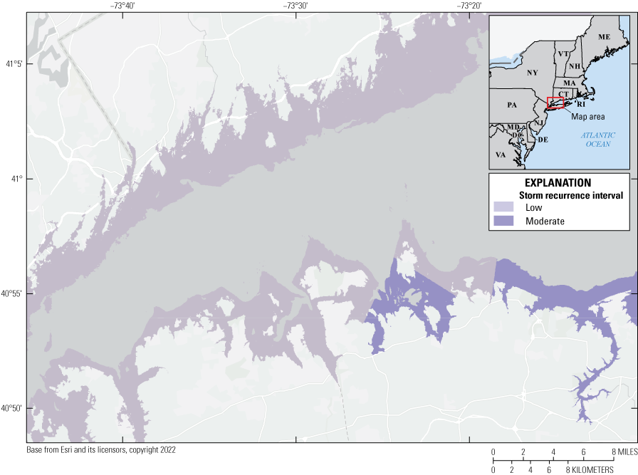
Map showing tropical storm recurrence interval, using historical storm track information from National Oceanic and Atmospheric Administration (Knapp and others, 2010) along the western side of Long Island Sound to highlight areas of the coast that have historically been more affected by tropical storms than other areas. Moderate storm recurrence intervals indicate areas that have four or more tropical storms per decade.
2.2.4.3. Erosion Hazard Data
USGS short-term shoreline change rates (Himmelstoss and others, 2010, 2018) were selected as an important estimator of future erosion hazards, because they capture more recent changes (during the past 30 to 40 years) of erosion, accretion, and engineering influences on coasts compared with the long-term erosion rates (during the past 50 or more years). The shoreline change transects from Himmelstoss and others (2010, 2018) were processed using the same methods described in the fabric dataset that used long-term shoreline change data (see section 2.1.5). End-point rates on transects with negative values (erosion hazards) were converted to raster and interpolation was used to fill small data gaps between the 50-m-spaced transects. Thresholds for erosion rates were defined as follows: less than −0.75 to 0 meter per year (m/yr) as low erosion, –3.0 to −0.75 m/yr as moderate erosion, and less than –3.0 m/yr as high erosion (fig. 20).
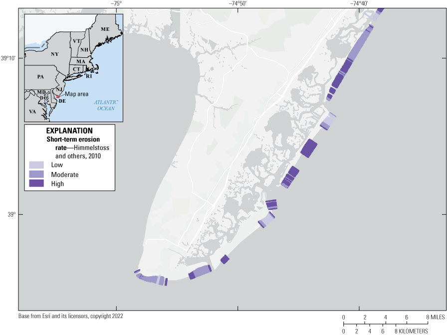
Map showing short-term erosion rates (Himmelstoss and others, 2010) on shore-perpendicular transects gridded for sandy open ocean coasts to highlight areas of the coast that are more and less likely to experience future erosion for the coastal area near Cape May, New Jersey, that is characterized as a series of barrier islands fronting back barrier saltmarshes. The erosion thresholds are defined in table 5.
2.3. CCL Outcomes: Supervised Classification of Fabric Plus Hazards
This section describes the process and classification schema for combining the fabric and hazards data. The overarching question that guided the creation of labeled classes in this step of this study was “Does this combination of landscape and hazard(s) make the coast more likely to change in the coming decade?”
As used in spatial analysis, supervised machine learning is a process by which users create training samples that identify characteristics of a phenomenon (in this case, combinations of fabric and hazards); these characteristics inform an algorithm that uses these samples as a reference to classify and create a new dataset. This new raster dataset is made up of pixels whose values are constrained by the training samples created by the user. The process of supervised classification is relatively straightforward once the number of classes and criteria for class assignment has been established.
Image classification in ArcGIS Pro (ver. 2.5) was the primary tool used to create the final CCL dataset. Fabric and hazards datasets were banded together as multilayer raster images, as is required for use in ArcGIS image classification. One banded image included the fabric dataset with the event hazards (tidal flooding, wave power, and storm overwash probability), and one included the fabric dataset with the perpetual hazards (relative sea level rise projections by 2030, short-term shoreline erosion, and storm recurrence interval). Supervised machine learning was used to assign labels to fabric and hazard combinations.
2.3.1. A Baseline for Estimating Hazard Impact
Establishing the criteria for classes relies on user knowledge of landscape and hazard interaction. For example, given a tidal flood event or a high wave event (or both), a bedrock coastal landscape is likely to remain unchanged; however, a forest or a wetland that experiences a high wave event or sea level rise flooding is likely to experience impacts that could result in landscape change. Using the ordinal hazard scale outlined in the hazard section, the relative effect of each possible hazard combination on each landscape type was estimated based on prior knowledge and expert opinion (supervision). Tables 6 and 7 outline the matrices that are used to create labeled classes that synthesize the hazard effects as a function of landscape type. Although the fabric tree scale discretizes beyond the landcover value (1 to 7, prior to subtrees, by landcover type), this classification step focuses just on the seven subaerial landscapes (rocky, hardened shores, developed, forested, wetlands, unconsolidated bluffs and beaches, and tidal flats).
Table 6.
The scale that creates labeled classes to combine event hazards and landscape type generated for the supervised machine learning process.[Event hazards include high tide flooding, wave power, and storm overwash probability. Hazard classifications are detailed in table 5]
Table 7.
The scale that creates labeled classes to combine perpetual hazards and landscape type for supervised machine learning process.[Perpetual hazards include storm frequency, relative sea level rise, and erosion. Hazard classifications are detailed in table 5]
2.3.2. Supervised Machine Learning
The CCL approach combines the fabric and the hazards data using supervised machine learning to identify relationships between the landscape and hazards; in other words, landscape and hazards are not independent variables, and not all hazards have the same degree of effect, allowing for the capture of different landscape hazard dependencies. For example, a category 2 storm on a barrier island does not have the same effect as a king tide on the same barrier island. Likewise, sea level rise will eventually turn a rocky intertidal zone into an aquatic seabed but may have limited effect on a sandy beach with an adequate sediment supply over the same timeframe. Furthermore, the weighting of hazards used in the supervised classification (tables 6 and 7) approach can be adjusted or refined without influencing the individual fabric or hazard datasets, making this framework flexible and updateable as knowledge of coastal landscape change increases given an associated increase in climate-driven coastal hazard effects.
Two individual sets of training samples were created to combine the landscape and hazards datasets for the supervised classification. For the fabric and event hazards dataset, 30 classes that represented combinations of landscapes and hazards were created for a total of 461 samples (fig. 21; table 6). For the fabric and perpetual hazards dataset, 25 classes that represented combinations of landscapes and hazards were created, for a total of 377 samples (fig. 22; table 7).
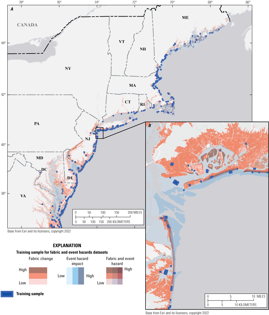
Map showing training sample locations used for the support vector machine supervised learning using the fabric and event hazards datasets for A, the northeastern United States and B, detail for Sandy Hook National Recreation Area in New Jersey and Fort Tilden (Gateway National Recreation Area) and Breezy Point Tip in New York.
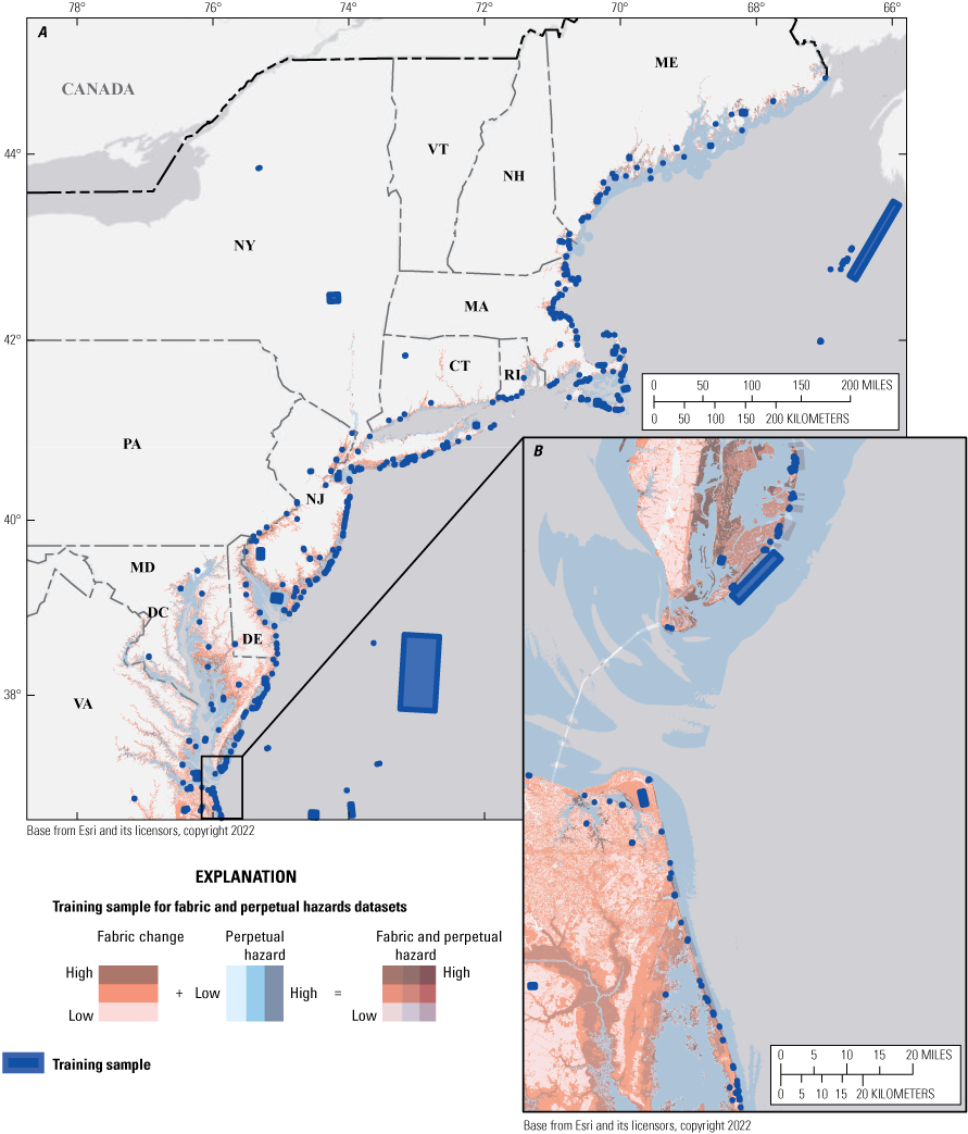
Map showing training sample locations used for the support vector machine supervised learning using the fabric and perpetual hazards datasets for A, the northeastern United States and B, detail for the mouth of the Chesapeake Bay in Virginia.
Once the class schema was established and training samples were created for each hazard type, the support vector machine classifier was used to create an 8-bit integer-value raster. In accordance with the schema in which training samples were created, the land cover type in the fabric dataset and the magnitude to which change likelihood would be increased (tables 6 and 7) were considered, and the latter served as an estimate of exposure based on the fabric dataset. Together, this fabric and hazard merged dataset provided ordinal-scale values to execute a modified version of the Glick and others (2011) equation (after Peek and others, 2022; see section 1.2) of sensitivity (fabric) plus exposure (hazard) refined with additional information to reflect the varying effects that a hazard or combinations of hazards will have across the landscape types (section 3). For example, an unconsolidated shore with high confidence shoreline change and high dunes has a fabric value of 7. If this landscape exists in an area that has a moderate shoreline erosion rate, moderate storm frequency, and is not expected to experience relative sea level rise, it will have a hazard-effect value of 2 for perpetual hazards. The combined CCL value is then the fabric value (7) plus the perpetual hazard value (2), resulting in a CCL value of 9. If the same unconsolidated shore (fabric value = 7) is in an area that experiences high storm overwash probability, then, with moderate wave power and likely high tide flooding, the event hazard effect value is 3, which would equate to a CCL value of 10 (fabric of 7 plus event hazard of 3). A final CCL raster is created by selecting the maximum CCL value from the two output rasters—event hazards and perpetual hazards—to capture the landscape-specific CCL due to all hazards (fig. 23). In the unconsolidated shore example, the maximum CCL value is 10. The ordinal scale of CCL is the same as the fabric ordinal scale (0-10), but CCL is either greater than or equal to the fabric value, because the CCL includes hazard information and is expressed in terms of high, low, or uncertain change likelihood (table 8).
Table 8.
Coastal change likelihood values and definitions for the outcomes of the framework for a coastal change likelihood assessment.[CCL dataset refers to the resistance or integrity of the coastal landscape and the hazards or combination of hazards that act on the landscape]
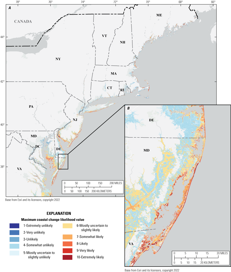
Map showing the maximum coastal change likelihood value derived from support vector machine supervised learning that combines the fabric data with the event and perpetual hazards and selects the maximum outcome of that combination for A, the northeastern United States and B, detail for an area along the Delmarva Peninsula that is characterized by developed and undeveloped barrier islands fronting saltmarshes.
Separate datasets for perpetual hazards and event hazards allow for examination of which type of hazard may have the greatest effect in certain areas based on user knowledge and intrinsic properties and hazards present. To better assess this, a derivative of the CCL supervised classification outputs was created by identifying threshold values within the event and hazard supervised learning outputs. For example, a CCL value of 8 indicates that coastal change is likely in that area in the next decade, whereas areas with values below this value, change is less likely. This determination allows distinguishing between the significance of event or perpetual hazards in influencing coastal change outcomes; areas with event outcomes above this threshold but perpetual outcomes below the threshold are likely dominated by event hazards, such as storms or tidal flooding. For areas dominated by perpetual hazards, change will be more likely linked to ongoing hazards, such as erosion or relative sea level rise. Areas with both event and perpetual hazards above the threshold are equally likely to experience change as a result of perpetual or event hazards, whereas those with both below the threshold are either more uncertain or not likely to change in response to these hazards in the next decade. Therefore, the final dataset created using these data is a raster data layer in which cell values range from 1 to 4, where a value of 1 corresponds to low event and low perpetual change expected, 2 corresponds to low event and high perpetual change expected, 3 corresponds to high event and low perpetual change expected, and 4 corresponds to high event and high perpetual change expected (fig. 24).
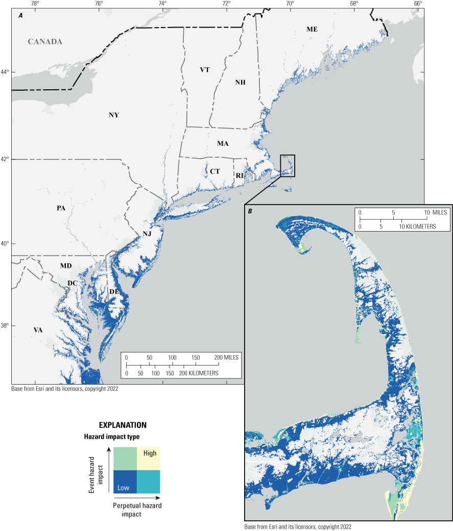
Map showing the hazards type layer, which highlights the hazard type (event or perpetual) that may be most influential in coastal change for A, the northeastern United States and B, detail for the outer extent of Cape Cod in eastern Massachusetts.
3. Data Access, Accuracy, and Limitations
3.1. Overview
This section describes the geospatial structure and distribution of the CCL datasets, how to access and ways to view the data, and their intended use. It also presents caveats and assessment accuracy, including limitations associated with source data, inconsistencies and misalignments associated with spatial data assimilation, and the gaps in data and knowledge.
3.2. Data Access
The fabric and hazards datasets of the CCL assessment and change likelihood outcomes are available in Sterne and others (2023). The CCL includes five GeoTIFFs: the fabric (section 2.1), the event and perpetual hazards (two GeoTIFFs; section 2.2), maximum CCL outcomes, and the event or perpetual hazard type indicator (section 2.3). These data can be updated as new and improved source data become available. Federal Geographic Data Committee-compliant metadata provided with each of the five CCL-related GeoTIFFs include detailed information on source data, definitions, geospatial processing and classification, references, and download instructions.
3.3. Data Viewing
The fabric geospatial dataset can be displayed in several ways using the attribute value table (.vat file) associated with the GeoTIFF. Data can be displayed by land cover classification (fig. 25), by fabric resistance value (prehazards; fig. 26), or by land cover specific decisions (figs. 7, 8, 9, 10, 11, 12, and 13). The hazard geospatial datasets can also be displayed in several ways. Perpetual (fig. 27) and event (fig. 28) hazards can be viewed according to their values (section 2.2), thresholds (figs. 15, 16, 17, 18, 19, and 20; section 2.2), or as combinations of hazards by using the attribute table associated with the hazard GeoTIFFs.
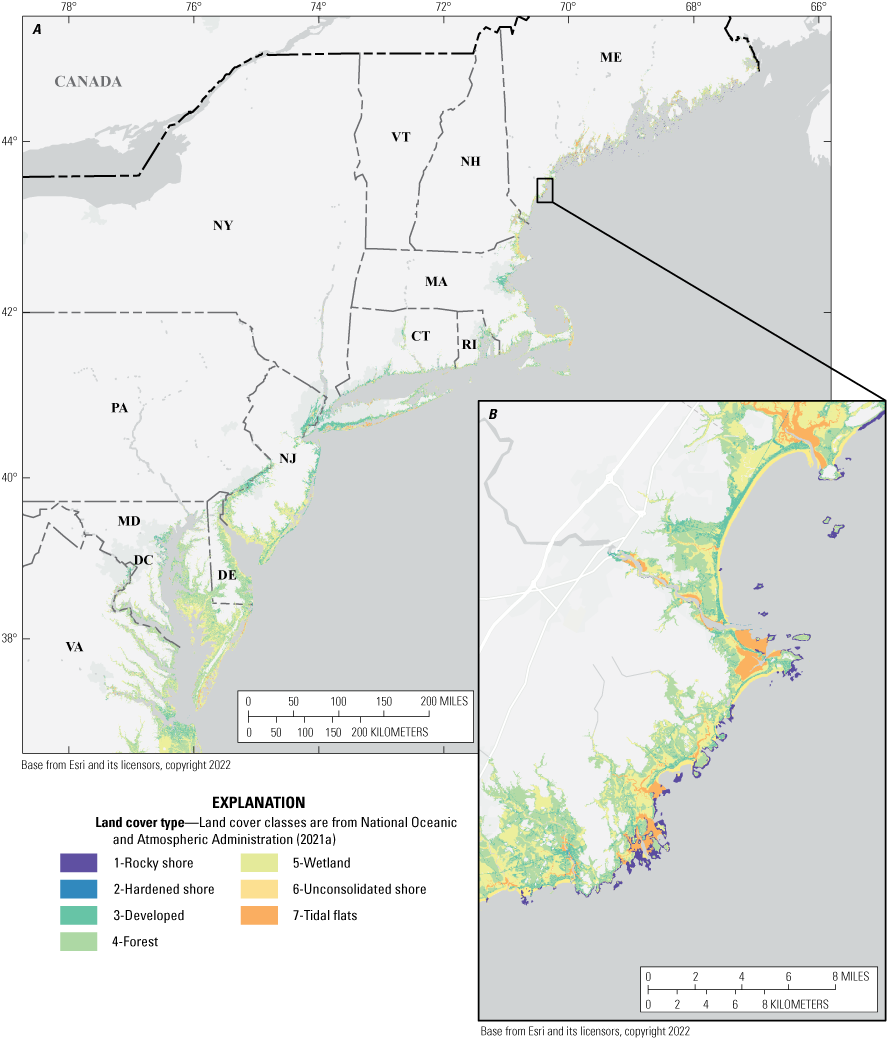
Maps showing the fabric dataset of the coastal change likelihood assessment pilot study, displayed by land cover type, for A, the northeastern United States and B, detail of the coastline of southern Maine.
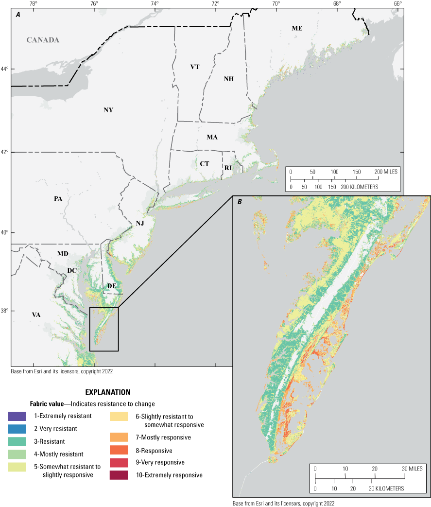
Maps showing the fabric dataset of the coastal change likelihood assessment pilot study, displayed by the fabric value, for A, the northeastern United States and B, detail for the southern extent of the Eastern Shore of Virginia near the mouth of the Chesapeake Bay. The fabric value is a measure of the inherent resistance of the landscape and is assigned after land cover-specific decisions have been made for the model, but before combining the landscape fabric data with the event and perpetual hazards datasets in the machine learning step.
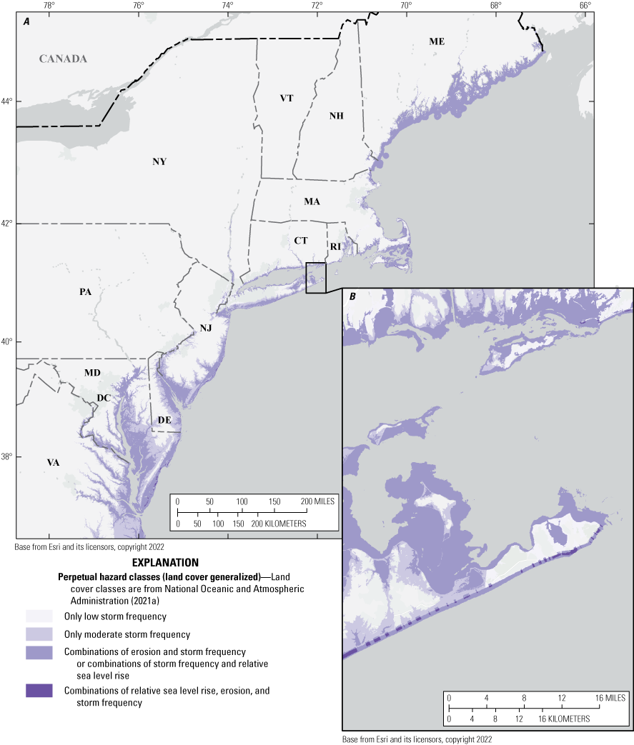
Maps showing perpetual hazard information in the coastal change likelihood assessment pilot study for A, the northeastern United States and B, detail of the eastern end of Long Island, New York. Perpetual hazard information is shown as single hazards and combinations of hazards using the coastal hazards classification (fig. 14).
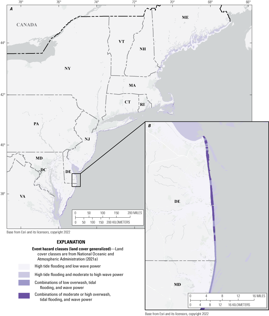
Maps showing event hazard information in the coastal change likelihood assessment pilot study for A, the northeastern United States and B, detail of the southern end of coastal Delaware. Event hazard information is shown as hazards and combinations of hazards using the coastal hazards classification (fig. 14).
The maximum CCL dataset can be displayed using the cell values that represent the maximum relative change likelihood (table 8) calculated when combining the support vector machine output from both the event and hazards datasets detailed in section 2.3 (figs. 21, 22, and 23; tables 6 and 7). The hazard type geospatial dataset can be displayed using the cell values that define which type of hazard a given location is most likely to be affected by (fig. 24).
3.3. Land Cover Accuracy
The overall accuracy of the eight primary land cover types is 80 percent (table 9), with a kappa coefficient of 0.77, which suggest good agreement between the land cover grouping of CCL and reference aerial imagery. The land cover classes derived from raster land cover sources had a producer’s accuracy—where pixels of a known class are classified as another class—of 81 percent. By contrast, the land cover classes that were derived from ESI vector data sources (National Oceanic and Atmospheric Administration, 2017, 2021b-g) had a producer’s accuracy of 85 percent. Water level differences in source imagery creates inaccuracies and inconsistencies in both the user and producer (ESI) accuracies for intertidal areas. No further accuracy assessments were conducted within the subtrees or hazard layers of this dataset. Comparing historical land cover change analyses to CCL outcomes produced through this methodology was beyond the parameters of the pilot study.
Table 9.
Confusion matrix for the land cover accuracy assessment.[Data are from Sterne and others (2023). Data are percentages of producer (rows) and user (columns) accuracy by land cover type. NA, not applicable]
Indicates landscape classes from environmental sensitivity index vector sources. All other classes are land cover derived from raster sources (see table 4 for land cover source information).
3.4. Limitations and Caveats
The CCL assessment and methods for the data build presented here serve as a first-order summary and analysis of intrinsic physical factors that characterize the coast and six common hazards that play a role in coastal change. This pilot study can be used as a decision support tool, a base layer for coastal landscape assessments, a synthesis of common coastal hazards, and a geospatial inventory of more than 20 source coastal geomorphic, remote sensing, topobathymetric, and oceanographic datasets. Although the resolution of this assessment was conducted at a 10-mpp scale, the intended scale of use is 1:10,000. Although pixel-level (10-mpp) detail is provided, this level of scrutiny should be used with caution. The intended scale of application of CCL is over the parcel level (>30 m) and should be used in conjunction with other data, tools, and local knowledge. This section describes details related to accuracy, and spatial and temporal scales. More information on individual layers (fabric, event and perpetual hazards, CCL, and hazard type) and their spatial and temporal accuracy can be found in the metadata of Sterne and others (2023).
3.5. Source Elevation Data
CONED (Danielson and others, 2018) was the preferred source of high-resolution seamless bathymetry and topography for the study area. However, CONED data were not available at the time of the polit study for areas north of Cape Ann, Mass. Additional digital elevation models (DEMs; Andrews and others, 2018; National Oceanic and Atmospheric Administration, 2021h) were added to the CONED to fill in gaps in the CCL domain in northern Massachusetts, New Hampshire, and Maine. The offshore domain in Maine and New Hampshire was approximated using the C–CAP domain extent due to a lack of high-resolution, seamless bathymetric data. Therefore, the domain does not uniformly represent the 10-m isobath contour in these two States. The CONED dataset has a root mean square error of 15 cm. The Massachusetts DEM (Andrews and others, 2018) has an assumed accuracy of better than 1 m, and the accuracy of the sea level rise DEMs from NOAA are considered accurate to 50 cm (National Oceanic and Atmospheric Administration, 2021h). Elevation data reflect the MHW elevation at the date of collection and are assumed to be current elevation, except within the relative sea level rise hazard estimate, which reflects elevation plus an estimate of sea level rise by 2030.
3.6. Source Land Cover Data
The beta version of the 10-m C–CAP land cover data (National Oceanic and Atmospheric Administration, 2021a) was the definitive source of land cover data wherever available. Alternative land cover data sources were used for New Jersey, Virginia, and Pennsylvania (along the Delaware River) where 10-m C–CAP data were not available (table 4). The change in the sources of land cover data created some seams along and within State boundaries as well as some differences in landscape classification. For example, the New Jersey land cover source associates recreational lands with urban landscapes, which is different than C–CAP, which associates green open space with undeveloped land cover. This difference in classification algorithm causes parts of New Jersey to appear more developed compared with other States and other land cover datasets. Land cover data for the Aberdeen, Md., proving ground military installation are masked for security purposes and have been given a “no data” classification, which is the same for the purposes of the CCL framework as the aquatic land cover class. A change in imagery date in the Maryland C–CAP data creates an unnatural boundary in the land cover data. The District of Columbia land cover is sourced from the Chesapeake Bay Program, as are parts of Pennsylvania along the Delaware River, and there are seams where different land cover sources meet up within the CCL domain. Land cover data reflect the land cover type at the date of imagery collection, which is between 2013 and 2017 for the data used in the fabric layer.
3.7. Source Shoreline-Type Data
Three land cover classes in this study were derived from NOAA ESI vector shoreline data (National Oceanic and Atmospheric Administration, 2017, 2021b-g). Both polyline and polygon datasets were rasterized and merged with the land cover source data. Some inconsistencies exist in the ESI data between the regional and national data products, and these can be seen in the landscape classification. For example, differences in the Maryland and Virginia and the Chesapeake Bay ESI datasets may result in overlapping or misaligned features (such as seawalls) in proximity. Spatial alignment issues arise from datum adjustments and shoreline source imagery year differences in the land cover data and the ESI data. Additionally, the rasterization of vector data can create irregularly or jagged shorelines when converted to pixels.
Although the translation of these vector shoreline feature classifications is not perfect, the overall benefit of including the three additional land cover classes from vector sources (rocky, hardened, and tidal flats) to support a comprehensive, regional change likelihood assessment far exceeds the limitations of the methods used to derive and incorporate them. Additionally, a seamless hardened shoreline database that classifies the type of hardened structure present (for example, pier, groin, jetty, bulkhead, seawall) is not currently available but exists along the Great Lakes (National Oceanic and Atmospheric Administration, 2022). This type of data source in the Northeast would add value to inform change likelihood within the hardened shore class in future assessments.
ESI data reflect the shoreline location and type at the date of imagery collection used to delineate shoreline features and attributes. The metadata for the fabric data layer of Sterne and others (2023) includes information about the source ESI ages.
3.8. Source Shoreline Change Data
The shoreline change rate data are more extensive for Massachusetts (Himmelstoss and others, 2018) than they are for other States in this study. Shoreline change data derived from the national assessment of shoreline change are only available along sandy, open ocean-facing coasts. However, the shoreline change data for Massachusetts often cover embayments, wetlands, and back barrier shorelines. This difference in data availability results in a more detailed assessment of shorelines in Massachusetts compared with other States. Additionally, shoreline change transects were edited in the national assessment dataset of Himmelstoss and others (2010) to prevent the transects from extending beyond the front side of the ocean coast. Transects lengths were more discrete and limited to the land cover area of interest in the Massachusetts dataset (Himmelstoss and others, 2018). Historic shoreline change trends are used in both the fabric and the hazards data layers. The long-term (>50 years) shoreline change metrics, specifically the 90 percent confidence interval, are applied to the fabric as intrinsic landscape properties, and the short-term (typically much less than 50 years) erosion rates are applied to the perpetual hazards layer.
3.9. Source UVVR Data
The UVVR data (Couvillion and others, 2021; Ganju and others, 2022) are the only fabric source data that did not exist at 10-mpp or finer resolution. The 30-mpp UVVR product was used in this study to resolve the decision nodes associated with salt marshes; the difference in resolution affects the apparent resolution of salt marshes where UVVR data were applied. UVVR data reflect the change in unvegetated-to-vegetated ratio between 2014 and 2018.
3.10. Source Hydrologic Units
Hydrologic units as defined in the USGS National Hydrography Dataset (U.S. Geological Survey, 2022) are used in the CCL framework to aggregate marsh elevation. Defne and Ganju (2016) outlined geospatial methods for assigning conceptual marsh units, but absent these units across the entire assessment domain, hydrologic basin segments are substituted from the HUC12 database (U.S. Geological Survey, 2022) to approximate an area within a contiguous marsh to represent a mean marsh elevation. This marsh elevation averaging approach was in close agreement with mean marsh elevations derived through conceptual marsh units in three marshes—Blackwater, Plum Island, and Chincoteague—outlined in Ganju and others (2020). Elevation data reflect the MHW elevation at the date of collection (table 4).
3.11. Source Dune Height and Storm Overwash Probability
Storm overwash probability and dune height metrics were sourced from Doran and others (2020). These data were joined to the shoreline change transects for ingestion into the CCL framework. There may be spatial misalignments associated with the geospatial conversion of these vector data from one container file to another. Dune heights reflect the light detection and ranging (lidar)-derived elevation of the source data at the date of collection.
3.12. Source Storm Recurrence
The storm recurrence dataset (Knapp and others, 2010) is for tropical storms only and therefore ignores the coastal change contributions that winter and extratropical storms have on the coastal landscape. To mitigate the tropical storm bias of this dataset, only two thresholds were established for storm recurrence, wherein the intent was to capture the difference between tropical storminess in the northern half of the study area compared with the southern half. The storm recurrence interval is based on storms from 1842 to the present, and the recurrence interval represents the number of storms per decade in a location for the past 150 or more years.
3.13. Source Relative Sea Level Rise Layer
Relative sea level rise is the only hazard used in this pilot study that consists of projected data. All other hazard layers used in this pilot study are based on recorded historical observations. The relative sea level rise or zone of possible inundation is created by adding an intermediate relative sea level rise (1 m by 2100) projection for 2030 (Sweet and others, 2017) to the DEM (Danielson and others, 2018; Andrews and others, 2018; National Oceanic and Atmospheric Administration, 2021h). A negative elevation bias of 15 cm (section 2.2.4.1) was included as well to offset the root mean square error of CONED, which accounts for more than 75 percent of the total domain. The effect zone of RSLR can be considered a maximum extent for 2030 because elevation errors were biased as being above MHW. Gesch (2012) would caution that the uncertainty associated with these elevation data is higher than the uncertainty associated with the RSLR projections for 2030 used for this study. For example, the CONED data have a root mean square error vertical accuracy of 15 cm and should not be used to estimate sea level rise inundation values less than about 58 cm. The perpetual hazard layer of relative sea level rise should be considered the layer with the most vertical positional uncertainty and used as a maximum surface that represented an area that could be affected by sea level rise in the next decade.
3.14. Source High Tide Flooding
Historical high tide flooding data (National Oceanic and Atmospheric Administration, 2020a) were resampled from their native resolution of about 3- to 10-mpp. This resampling of flood extent can create slight offsets (less than 5-m horizontal positional accuracy) along the wet/dry boundary. High tide flooding is a historical record of high-water lines measured on land and at tidal gage locations.
3.15. Source Wave Power
Climatological wave power (Aretxabaleta and others, 2022) was interpolated from a finite element grid. These data were interpolated to the extent of the high tide flood layer to approximate the maximum extent of wave propagation onto a flooded landscape. Interpolation by nearest neighbor was used to transform the wave power data onto the 10-mpp assessment domain. Climatological wave powers are based on model simulations between 2000 and 2018 (Aretxabaleta and others, 2022), and therefore we assume that past climatological wave power will be similar to wave power in the coming decade.
4. Summary
The U.S. Geological Survey, under the auspices of the Natural Resource Preservation Program and in cooperation with the National Park Service, compiled previously published data from numerous agencies to investigate the coastal landscape change likelihood to support archeological resource management in national parks. This report presents a methodology to assess coastal change likelihood and a pilot study of the methodology for the northeastern U.S. These data products include the fabric dataset, which summarizes coastal landforms between −10 and +10 m relative to the Mean High Water datum and an estimate of the likelihood of these landforms to change as a function of their intrinsic physical properties, shear strength, and resistance to change; two hazards data layers (event and perpetual hazards) that provide a synthesis of six common coastal hazards that are likely to affect the coastal landscape in the coming decade; a combined estimate of change likelihood according to both hazard types as a function of landscape-type and the hazards present and their magnitude; and an assessment of hazard types (event, perpetual, or both) most likely to influence coastal change. The data can be used to support near-term (approximately 10 years) decision making in the coastal zone and are intended to be used in conjunction with other data and expertise. When combined with stakeholder knowledge, the results of this study provide a tool to gage climate effects on coastal infrastructure and identify where critical habitats and resources are in danger of disappearing in response to coastal hazards.
The coastal change likelihood assessment is a computer-aided interpretation of the coastal landscape and the hazards that act on it. The outcomes provide a flexible framework that indicates where the myriads of factors that influence coastal change across a variety of landscapes exist; these outcomes can be used to support decision making in the coastal zone, including but not limited to informing and identifying areas for further investigation, baseline data to inform asset and resource vulnerability assessments, and to help prioritize scientific research data and knowledge needs regarding the future physical landscape response to coastal hazards.
5. Selected References
Andrews, B.D., Baldwin, W.E., Sampson, D.W., and Schwab, W.C., 2018, Continuous bathymetry and elevation models of the Massachusetts coastal zone and continental shelf (ver. 3.0, December 2019): U.S. Geological Survey data release, accessed September 19, 2022, at https://doi.org/10.5066/F72806T7.
Aretxabaleta, A.L., Defne, Z., Kalra, T.S., Blanton, B.O., and Ganju, N.K., 2022, Climatological wave height, wave period and wave power along coastal areas of the east coast of the United States and Gulf of Mexico: U.S. Geological Survey data release, accessed September 19, 2022, at https://doi.org/10.5066/P9HJ0JIQ.
Boudreaux, J.P., 2012, Shear strength evaluation of an erosional soil system at Fourchon Beach: Louisiana State University thesis, 118 p., accessed August 2022 at https://core.ac.uk/download/pdf/217403683.pdf.
Chesapeake Conservancy, 2018, Landcover data project 2013/2014: Chesapeake Conservancy web page, accessed September 19, 2022, at https://www.chesapeakeconservancy.org/conservation-innovation-center/high-resolution-data/land-cover-data-project/.
Couvillion, B.R., Ganju, N.K., and Defne, Z., 2021, An unvegetated to vegetated ratio (UVVR) for coastal wetlands of the conterminous United States (2014–2018): U.S. Geological Survey data release, accessed September 19, 2022, at https://doi.org/10.5066/P97DQXZP.
Danielson, J.J., Poppenga, S.K., Tyler, D.J., Palaseanu-Lovejoy, M., and Gesch, D.B., 2018, Coastal national elevation database: U.S. Geological Survey Fact Sheet 2018–3037, 2 p., accessed September 19, 2022, at https://doi.org/10.3133/fs20183037.
Defne, Z., and Ganju, N.K., 2016, Conceptual salt marsh units for wetland synthesis: Edwin B. Forsythe National Wildlife Refuge, New Jersey: U.S. Geological Survey data release, accessed September 19, 2022, at https://doi.org/10.5066/F7QV3JPG.
Defne, Z., Aretxabaleta, A.L., Ganju, N.K., Kalra, T.S., Jones, D.K., and Smith, K.E.L., 2020, A geospatially resolved wetland vulnerability index—Synthesis of physical drivers: PLoS One, v. 15, no. 1, paper e0228504, 27 p., accessed September 19, 2022, at https://doi.org/10.1371/journal.pone.0228504.
Doran, K.S., Birchler, J.J., Hardy, M.W., Bendik, K.J., Pardun, J.M., and Locke, H.A., 2020, National assessment of hurricane-induced coastal erosion hazards (ver. 2.0, February 2021): U.S. Geological Survey data release, accessed September 19, 2022, at https://doi.org/10.5066/P99ILAB9.
Dupigny-Giroux, L.A., Mecray, E.L., Lemcke-Stampone, M.D., Hodgkins, G.A., Lentz, E.E., Mills, K.E., Lane, E.D., Miller, R., Hollinger, D.Y., Solecki, W.D., Wellenius, G.A., Sheffield, P.E., MacDonald, A.B., and Caldwell, C., 2018, Northeast, chap. 18 of Reidmiller, D.R., Avery, C.W., Easterling, D.R., Kunkel, K.E., Lewis, K.L.M., Maycock, T.K., and Stewart, B.C., eds., Impacts, risks, and adaptation in the United States: U.S. Global Change Research Program Fourth National Climate Assessment, v. II, p. 669–742, accessed November 17, 2022, at https://doi.org/10.7930/NCA4.2018.CH18.
Emery, K.O., and Aubrey, D.G., 1991, Sea levels, land levels, and tide gauges: New York, Springer-Verlag, 237 p. [Also available at https://doi.org/10.1007/978-1-4613-9101-2.]
Emery, K.O., and Uchupi, E., 1984, The geology of the Atlantic Ocean: New York, Springer-Verlag, 1,050 p. [Also available at https://doi.org/10.1007/978-1-4612-5278-8.]
Esri, 2020a, ArcGIS Pro 2.6 patch 3 is available: Esri community web page, accessed June 21, 2021, at https://community.esri.com/t5/arcgis-pro-documents/arcgis-pro-2-6-patch-3-is-available/ta-p/918428.
Esri, 2020b, What is ArcPy?: Esri web page, accessed June 21, 2021, at https://pro.arcgis.com/en/pro-app/latest/arcpy/get-started/what-is-arcpy-.htm.
Ganju, N.K., Couvillion, B.R., Defne, Z., and Ackerman, K.V., 2022, Development and application of Landsat-based wetland vegetation cover and unvegetated-vegetated marsh ratio (UVVR) for the conterminous United States: Estuaries and Coasts, May 2, 18 p., accessed September 19, 2022, at https://doi.org/10.1007/s12237-022-01081-x.
Ganju, N.K., Defne, Z., and Fagherazzi, S., 2020, Are elevation and open‐water conversion of salt marshes connected?: Geophysical Research Letters, v. 47, no. 3, paper e2019GL086703, 10 p., accessed September 19, 2022, at https://doi.org/10.1029/2019GL086703.
Ganju, N.K., Defne, Z., Kirwan, M.L., Fagherazzi, S., D’Alpaos, A., and Carniello, L., 2017a, Spatially integrative metrics reveal hidden vulnerability of microtidal salt marshes: Nature Communications, v. 8, article 14156, 7 p., accessed November 15, 2022, at https://doi.org/10.1038/ncomms14156.
Ganju, N.K., Suttles, S.E., Beudin, A., Nowacki, D.J., Miselis, J.L., and Andrews. B.D., 2017b, Quantification of storm-induced bathymetric change in a back-barrier estuary: Estuaries and Coasts, v. 40, no. 1, p. 22–36., accessed November 15, 2022, at https://doi.org/10.1007/s12237-016-0138-5.
Gesch, D.B., 2009, Analysis of lidar elevation data for improved identification and delineation of lands vulnerable to sea level rise: Journal of Coastal Research, v. 10053, special issue 53, p. 49–58, accessed September 20, 2022, at https://doi.org/10.2112/SI53-006.1.
Gesch, D.B., 2012, Elevation uncertainty in coastal inundation hazard assessments, chap. 6 of Cheval, S., ed., Natural disasters: IntechOpen, p. 121–140, accessed August 20, 2022, at https://doi.org/10.5772/31972.
Glick, P., Stein, B.A., and Edelson, N.A., eds., 2011, Scanning the conservation horizon—A guide to climate change vulnerability assessment: National Wildlife Federation, 168 p., accessed September 20, 2022, at https://www.nwf.org/~/media/pdfs/global-warming/climate-smart-conservation/nwfscanningtheconservationhorizonfinal92311.ashx.
Gornitz, V., 1990, Vulnerability of the east coast, U.S.A. to future sea level rise, in Proceedings of the Skagen Symposium (2–5 September 1990): Journal of Coastal Research, special issue 9, p. 201–237, accessed September 20, 2022, at https://www.jstor.org/stable/44868636.
Himmelstoss, E.A., Farris, A.S., and Weber, K.M., 2018, Massachusetts shoreline change project, 2018 update—A GIS compilation of shoreline change rates calculated using Digital Shoreline Analysis System version 5.0, with supplementary intersects and baselines for Massachusetts: U.S. Geological Survey data release, accessed September 20, 2022, at https://doi.org/10.5066/P9RRBEYK.
Himmelstoss, E.A., Kratzmann, M., Hapke, C., Thieler, E.R., and List, J., 2010, The national assessment of shoreline change—A GIS compilation of vector shorelines and associated shoreline change data for the New England and mid-Atlantic coasts: U.S. Geological Survey Open-File Report 2010–1119, accessed September 20, 2022, at https://doi.org/10.3133/ofr20101119.
Intergovernmental Panel on Climate Change, 2014, Climate change 2014—Impacts, adaptation, and vulnerability—Summary for policymakers, in Field, C.B., ed., Contribution of Working Group II to the fifth assessment report: Intergovernmental Panel on Climate Change, 32 p., accessed September 20, 2022, at https://www.ipcc.ch/site/assets/uploads/2018/02/ar5_wgII_spm_en.pdf.
Intergovernmental Panel on Climate Change, 2021, Climate change 2021—The physical science basis, in Masson-Delmotte, V., Zhai, P., Pirani, A., Connors, S.L., Péan, C., Berger, S., Caud, N., Chen, Y., Goldfarb, L., Gomis, M.I., Huang, M., Leitzell, K., Lonnoy, E., Matthews, J.B.R., Maycock, T.K., Waterfield, T., Yelekçi, O., Yu, R., and Zhou, B., eds., Working Group I contribution to the IPCC sixth assessment report: Intergovernmental Panel on Climate Change, 2,391 p., accessed September 20, 2022, at https://doi.org/10.1017/9781009157896.
Jafari, N.H., Harris, B.D., Cadigan, J.A., Day, J.W., Sasser, C.E., Kemp, G.P., Wigand, C., Freeman, A., Sharp, L.A., Pahl, J., Shaffer, G.P., Holm, G.O., Jr, and Lane, R.R., 2019, Wetland shear strength with emphasis on the impact of nutrients, sediments, and sea level rise: Estuarine, Coastal, and Shelf Science, v. 229, article 106394, 27 p., accessed September 20, 2022, at https://doi.org/10.1016/j.ecss.2019.106394.
Jupyter, 2020, Jupyter: Jupyter software, accessed June 21, 2021, at https://jupyter.org/.
Kirwan, M.L., and Gedan, K.B., 2019, Sea level driven land conversion and the formation of ghost forests: Nature Climate Change, v. 9, p. 450–457, accessed September 20, 2022, at https://doi.org/10.1038/s41558-019-0488-7. [Author correction published at https://doi.org/10.1038/s41558-019-0568-8.]
Knapp, K.R., Kruk, M.C., Levinson, D.H., Diamond, H.J., and Neumann, C.J., 2010, The international best track archive for climate stewardship (IBTrACS)—Unifying tropical cyclone best track data: Bulletin of the American Meteorological Society, v. 91, no. 3, p. 363–376, accessed September 20, 2022, at https://doi.org/10.1175/2009BAMS2755.1.
Lentz, E.E., Stippa, S.R., Thieler, E.R., Plant, N.G., Gesch, D.B., and Horton, R.M., 2015, Evaluating coastal landscape response to sea level rise in the northeastern United States—Approach and methods (ver. 2.0, December 2015): U.S. Geological Survey Open-File Report 2014–1252, 27 p., accessed September 20, 2022, at https://doi.org/10.3133/ofr20141252.
Lentz, E.E., Thieler, E.R., Plant, N.G., Stippa, S.R., Horton, R.M., and Gesch, D.B., 2016, Evaluation of dynamic coastal response to sea level rise modifies inundation likelihood: Nature Climate Change, v. 6, p. 696–700, accessed September 20, 2022, at https://doi.org/10.1038/nclimate2957.
Mariotti, G., Fagherazzi, S., Wiberg, P.L., McGlathery, K.J., Carniello, L., and Defina, A., 2010, Influence of storm surges and sea level on shallow tidal basin erosive processes: Journal of Geophysical Research, v. 115, no. C11, article C11012, 17 p., accessed September 20, 2022, at https://doi.org/10.1029/2009JC005892.
McGarigal, K., Compton, B.W., Plunkett, E.B., DeLuca, W.V., and Grand, J., 2020, Designing sustainable landscapes: University of Massachusetts Amherst project website, accessed September 20, 2022, at http://umassdsl.org/.
Molino, G.D., Kennedy, M.A., and Sutton-Grier, A.E., 2020, Stakeholder-defined scientific needs for coastal resilience decisions in the northeast U.S: Marine Policy, v. 118, article 103987, 10 p., accessed September 20, 2022, at https://doi.org/10.1016/j.marpol.2020.103987.
Moore, R.B., McKay, L.D., Rea, A.H., Bondelid, T.R., Price, C.V., Dewald, T.G., and Johnston, C.M., 2019, User’s guide for the national hydrography dataset plus (NHDPlus) high resolution: U.S. Geological Survey Open-File Report 2019–1096, 66 p., https://doi.org/10.3133/ofr20191096.
National Geophysical Data Center, 1988, Digital relief of the surface of the Earth—Data announcement 88–MGG–02: National Geophysical Data Center digital data, accessed September 19, 2022, at https://www.ngdc.noaa.gov/mgg/global/etopo5.HTML.
National Oceanic and Atmospheric Administration, 2017, Environmental sensitivity index (ESI) maps and data: National Oceanic and Atmospheric Administration data, accessed September 20, 2022, at https://response.restoration.noaa.gov/esi.
National Oceanic and Atmospheric Administration, 2018, What are the chances a hurricane will hit my home?: National Oceanic and Atmospheric Administration web page, accessed August 2022 at https://www.noaa.gov/stories/what-are-chances-hurricane-will-hit-my-home.
National Oceanic and Atmospheric Administration, 2019, Derived C–CAP land cover data [beta]: National Oceanic and Atmospheric Administration C–CAP Regional Land Cover and Change website, accessed January 2021 at https://www.coast.noaa.gov/htdata/raster1/landcover/bulkdownload/.
National Oceanic and Atmospheric Administration, 2020a, Coastal flood frequency: National Oceanic and Atmospheric Administration Digital Coast website, accessed September 20, 2022, at https://coast.noaa.gov/digitalcoast/data/floodfrequency.html.
National Oceanic and Atmospheric Administration, 2020b, VDatum (version 4.3): National Oceanic and Atmospheric Administration software tool, accessed January 2022, at http://vdatum.noaa.gov.
National Oceanic and Atmospheric Administration, 2021a, C–CAP derived land cover—Beta: National Oceanic and Atmospheric Administration data, accessed November 16, 2022, at https://coast.noaa.gov/digitalcoast/data/ccapderived.html.
National Oceanic and Atmospheric Administration, 2021b, Chesapeake Bay and the outer coasts of Maryland and Virginia 2016 ESI polygons [2010–06–15 to 2010–08–15]: National Oceanic and Atmospheric Administration dataset, accessed September 20, 2022, at https://www.fisheries.noaa.gov/inport/item/40644.
National Oceanic and Atmospheric Administration, 2021c, Delaware/New Jersey/Pennsylvania 2014 ESI polygons [2010–06–15 to 2010–08–15]: National Oceanic and Atmospheric Administration dataset, accessed September 20, 2022, at https://www.fisheries.noaa.gov/inport/item/53861.
National Oceanic and Atmospheric Administration, 2021d, Long Island Sound 2016 ESI polygons [2010–06–15 to 2010–08–15]: National Oceanic and Atmospheric Administration dataset, accessed September 20, 2022, at https://www.fisheries.noaa.gov/inport/item/40470.
National Oceanic and Atmospheric Administration, 2021e, Maine and New Hampshire 2016 ESI polygons [2010–06–15 to 2010–08–15]: National Oceanic and Atmospheric Administration dataset, accessed September 20, 2022, at https://www.fisheries.noaa.gov/inport/item/40371.
National Oceanic and Atmospheric Administration, 2021f, Massachusetts and Rhode Island 2016 ESIP (ESI shoreline types—Polygons) [2010–06–15 to 2010–08–15]: National Oceanic and Atmospheric Administration dataset, accessed September 20, 2022, at https://www.fisheries.noaa.gov/inport/item/51698.
National Oceanic and Atmospheric Administration, 2021g, NY/NJ metro area, Hudson River, and south Long Island 2016 ESIP (environmental sensitivity index polygons) [2010–06–15 to 2010–08–15]: National Oceanic and Atmospheric Administration dataset, accessed September 20, 2022, at https://www.fisheries.noaa.gov/inport/item/40466.
National Oceanic and Atmospheric Administration, 2021h, Sea level rise data download: National Oceanic and Atmospheric Administration data, accessed September 20, 2022, at https://coast.noaa.gov/slrdata/.
National Oceanic and Atmospheric Administration, 2022, Great lakes hardened shorelines classification 2019: National Oceanic and Atmospheric Administration dataset, accessed September 20, 2022, at https://www.fisheries.noaa.gov/inport/item/59439.
National Park Service, 2022, NPS—Land Resources Division boundary and tract data service: National Park Service data, accessed November 15, 2022, at https://public-nps.opendata.arcgis.com/maps/c8d60ffcbf5c4030a17762fe10e81c6a/about.
National Research Council, 2007, Elevation data for floodplain mapping: National Academy of Sciences, 151 p., accessed November 15, 2022, at https://doi.org/10.17226/11829.
Neumann, B., Vafeidis, A.T., Zimmermann, J., and Nicholls, R.J., 2015, Future coastal population growth and exposure to sea level rise and coastal flooding—A global assessment: PLoS One, v. 10, no. 3, article e0118571, 34 p., accessed September 20, 2022, at https://doi.org/10.1371/journal.pone.0118571.
New Jersey Department of Environmental Protection Bureau of GIS, 2019, Land use/land cover of New Jersey 2015: New Jersey Department of Environmental Protection data, accessed September 20, 2022, at https://gisdata-njdep.opendata.arcgis.com/documents/6f76b90deda34cc98aec255e2defdb45/about.
Onasch, C., 2010, Some useful numbers on the engineering properties of materials (geologic and otherwise): Pennsylvania State University Geology 615 notes, 6 p., accessed November 7, 2022, at https://cpb-us-e1.wpmucdn.com/sites.psu.edu/dist/1/57960/files/2016/10/Some-Useful-Numbers-1g1rkuu.pdf.
Osman, N., and Barakbah, S.S., 2006, Parameters to predict slope stability—Soil water and root profiles: Ecological Engineering, v. 28, no. 1, p. 90–95, accessed September 20, 2022, at https://doi.org/10.1016/j.ecoleng.2006.04.004.
Peek, K., Tormey, B., Thompson, H., Young, R., Norton, S., McNamee, J., and Scavo, R., 2017, Coastal hazards & sea level rise asset vulnerability assessment & tsunami vulnerability case study: National Park Service, 28 p., accessed September 20, 2022, at https://doi.org/10.36967/2293653.
Peek, K.M., Tormey, B.R., Thompson, H.L., and Young, R.S., 2022, Coastal hazards & climate change asset vulnerability assessment protocol—Updated protocol description & methodology: National Park Service National Resource Report 2022/2427, 45 p., accessed September 20, 2022, at https://doi.org/10.36967/2293653.
Ricci, G., Robadue, D.D., Jr., Rubinoff, P., Casey, A., and Babson, A.L., 2019, Integrated coastal climate change vulnerability assessment—Colonial National Historical Park: National Park Service Natural Resource Report NPS/COLO/NRR—2019/1945, 308 p., accessed September 20, 2022, at https://irma.nps.gov/DataStore/Reference/Profile/2264709.
Ricci, G., Robadue, D.D., Jr., Rubinoff, P., Casey, A., and Babson, A.L., 2020, Integrated coastal climate change vulnerability assessment—Fire Island National Seashore: National Park Service Natural Resource Report NPS/FIIS/NRR—2020/2156, 192 p., accessed September 20, 2022, at https://irma.nps.gov/DataStore/Reference/Profile/2276834.
Sallenger, A.H., Jr., 2000, Storm impact scale for barrier islands: Journal of Coastal Research, v. 16, no. 3, p. 890–895, accessed September 20, 2022, at https://www.jstor.org/stable/4300099.
Shaw, J., Taylor, R.B., Forbes, D.L., Ruz, M.-H., and Solomon, S., 1998, Sensitivity of the coasts of Canada to sea level rise: Geological Survey of Canada Bulletin 505, 79 p., accessed September 20, 2022, at https://publications.gc.ca/collections/collection_2017/rncan-nrcan/M42-505-eng.pdf.
Sterne, T.K., Pendleton, E.A., Lentz, E.E., and Henderson, R.E., 2023, Coastal change likelihood in the U.S. northeast region—Maine to Virginia: U.S. Geological Survey data release, https://doi.org/10.5066/P96A2Q5X.
Stockdon, H.F., Doran, K.J., Thompson, D.M., Sopkin, K.L., Plant, N.G., and Sallenger, A.H., 2012, National assessment of hurricane-induced coastal erosion hazards—Gulf of Mexico: U.S. Geological Survey Open-File Report 2012–1084, 51 p., accessed September 20, 2022, at https://doi.org/10.3133/ofr20121084.
Sweet, W.V., Kopp, R.E., Weaver, C.P., Obeysekera, J., Horton, R.M., Thieler, E.R., and Zervas, C., 2017, Global and regional sea level rise scenarios for the United States: National Oceanic and Atmospheric Administration Technical Report NOS CO–OPS 083, 75 p., accessed September 20, 2022, at https://tidesandcurrents.noaa.gov/publications/techrpt83_Global_and_Regional_SLR_Scenarios_for_the_US_final.pdf.
Thieler, E.R., and Hammar-Klose, E.S., 1999, National assessment of coastal vulnerability to sea level rise; U.S. Atlantic Coast: U.S. Geological Survey Open-File Report 99–593, accessed September 20, 2022, at https://doi.org/10.3133/ofr99593.
Twomey, E.R., and Signell, R.P., 2013, Construction of a 3-arcsecond digital elevation model for the Gulf of Maine: U.S. Geological Survey Open-File Report 2011–1127, 24 p., accessed September 20, 2022, at https://doi.org/10.3133/ofr20111127.
U.S. Fish and Wildlife Service, 2020, National wetlands inventory website: U.S. Fish and Wildlife Service database, accessed September 20, 2022, at http://www.fws.gov/wetlands/.
U.S. Geological Survey, 2020, National hydrography dataset plus high resolution (NHDPlus HR) availability map: U.S. Geological Survey Watershed Boundary Dataset, accessed September 20, 2022, at https://usgs.maps.arcgis.com/apps/MapTools/index.html?appid=41a5c2ca49bd4a83b239450e61022d53.
U.S. Geological Survey, 2022, National hydrography dataset: U.S. Geological Survey data, accessed November 16, 2022, at https://www.usgs.gov/national-hydrography/national-hydrography-dataset.
University of Vermont Spatial Analysis Laboratory, 2017, High-resolution land cover, state of New Jersey, Delaware River basin, 2013–2017: University of Vermont Spatial Analysis Laboratory dataset, accessed September 20, 2022, at http://www.pasda.psu.edu/uci/DataSummary.aspx?dataset=3147.
Virginia Geographic Information Network, 2020, 1-meter Virginia land cover, raster digital data: Virginia Geographic Information Network dataset, accessed September 20, 2022, at https://vgin.vdem.virginia.gov/pages/clearinghouse. [Direct access to the data from https://vgin.maps.arcgis.com/home/item.html?id=6ae731623ff847df91df767877db0eae; VGIN ArcGIS Online account required.]
Ward, N.D., Megonigal, J.P., Bond-Lamberty, B., Bailey, V.L., Butman, D., Canuel, E.A., Diefenderfer, H., Ganju, N.K., Goñi, M.A., Graham, E.B., Hopkinson, C.S., Khangaonkar, T., Langley, J.A., McDowell, N.G., Myers-Pigg, A.N., Neumann, R.B., Osburn, C.L., Price, R.M., Rowland, J., Sengupta, A., Simard, M., Thornton, P.E., Tzortziou, M., Vargas, R., Weisenhorn, P.B., and Windham-Myers, L., 2020, Representing the function and sensitivity of coastal interfaces in earth system models: Nature Communications, v. 11, article 2458, 14 p., accessed September 20, 2022, at https://doi.org/10.1038/s41467-020-16236-2.
Wessel, P., and Smith, W.H.F., 1996, A global, self-consistent, hierarchical, high-resolution shoreline database: Journal of Geophysical Research: Solid Earth, v. 101, no. B4, p. 8741–8743, accessed September 20, 2022, at https://doi.org/10.1029/96JB00104.
Western Carolina University and National Park Service, 2016, Coastal hazards & climate change asset vulnerability assessment protocol—Protocol description and methodology: National Park Service, 6 p., accessed September 20, 2022, at https://irma.nps.gov/DataStore/DownloadFile/649325.
Appendix 1. Coastal Change Likelihood in the Northeastern United States
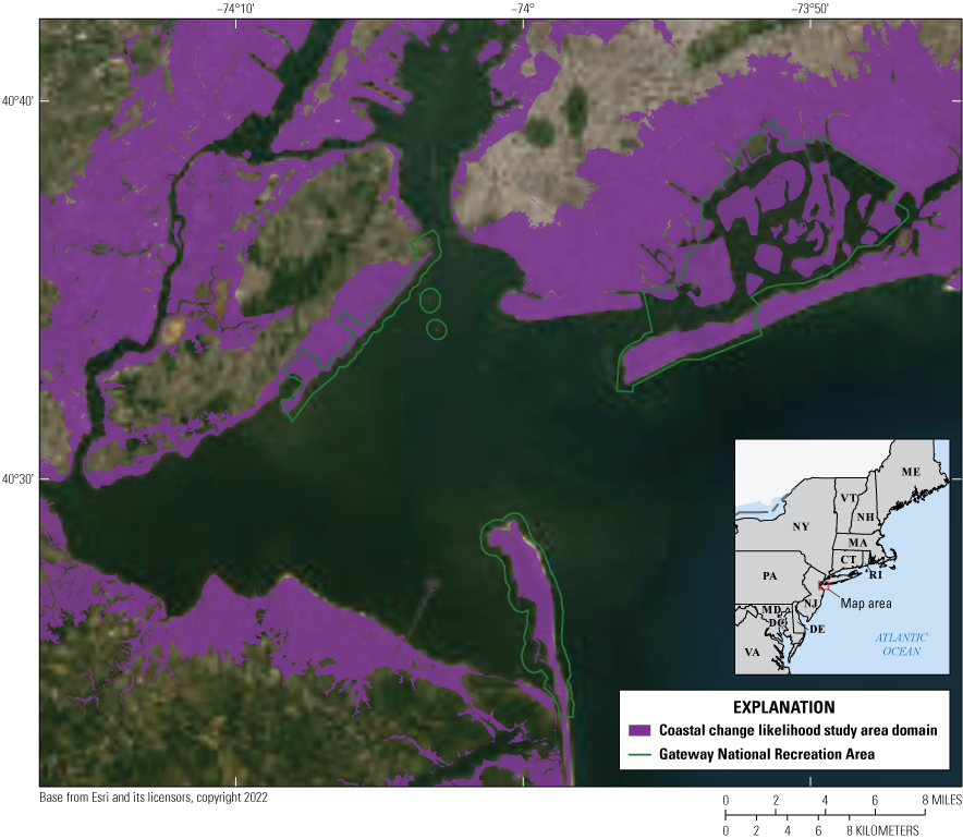
Map showing Gateway National Recreation Area in New York and New Jersey, used to illustrate the pilot study of the methodology of a coastal change likelihood assessment.
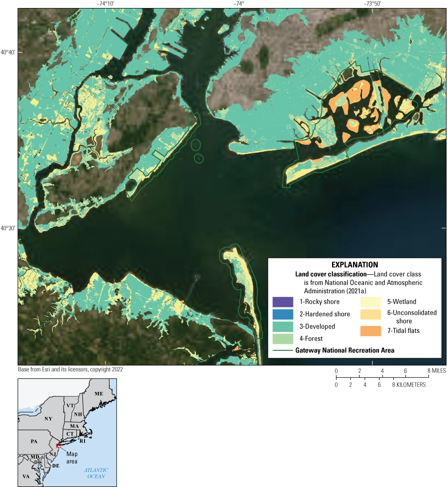
Map showing land cover, which forms the foundation of the fabric data, for Gateway National Recreation Area in New York and New Jersey, used as part of the pilot study of the methodology of a coastal change likelihood assessment.
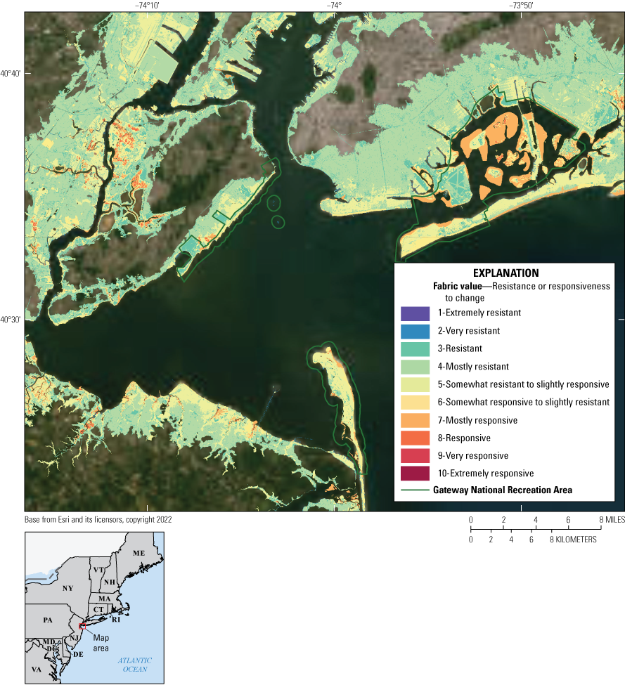
Map showing responsiveness (or conversely, resistance) of landscapes in Gateway National Recreation Area in New York and New Jersey, as part of the pilot study of the methodology of a coastal change likelihood assessment. Fabric value is determined through a decision tree framework that considers the land cover type and intrinsic properties of the landscape that affects its ability to resist change.
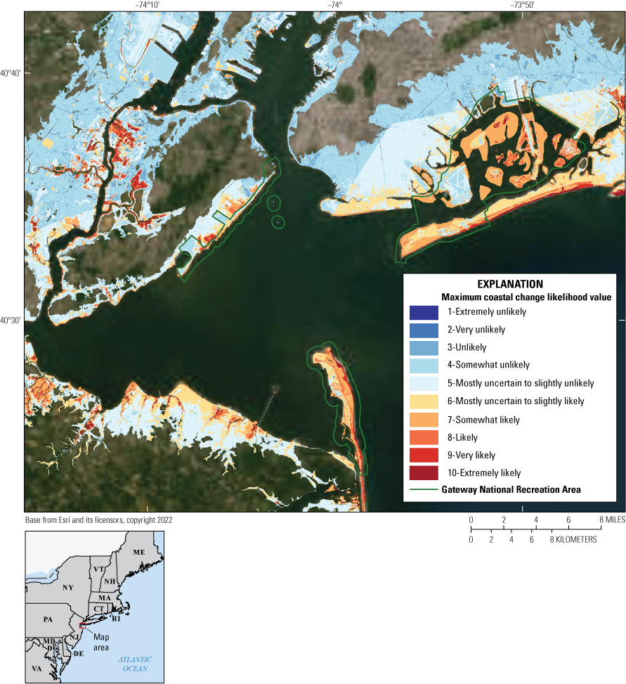
Map showing coastal change likelihood in Gateway National Recreation Area in New York and New Jersey, as part of the pilot study of the methodology of a coastal change likelihood assessment. The maximum coastal change likelihood value derived from support vector machine supervised learning combines the fabric data with the event and perpetual hazards and selects the maximum outcome of that combination.
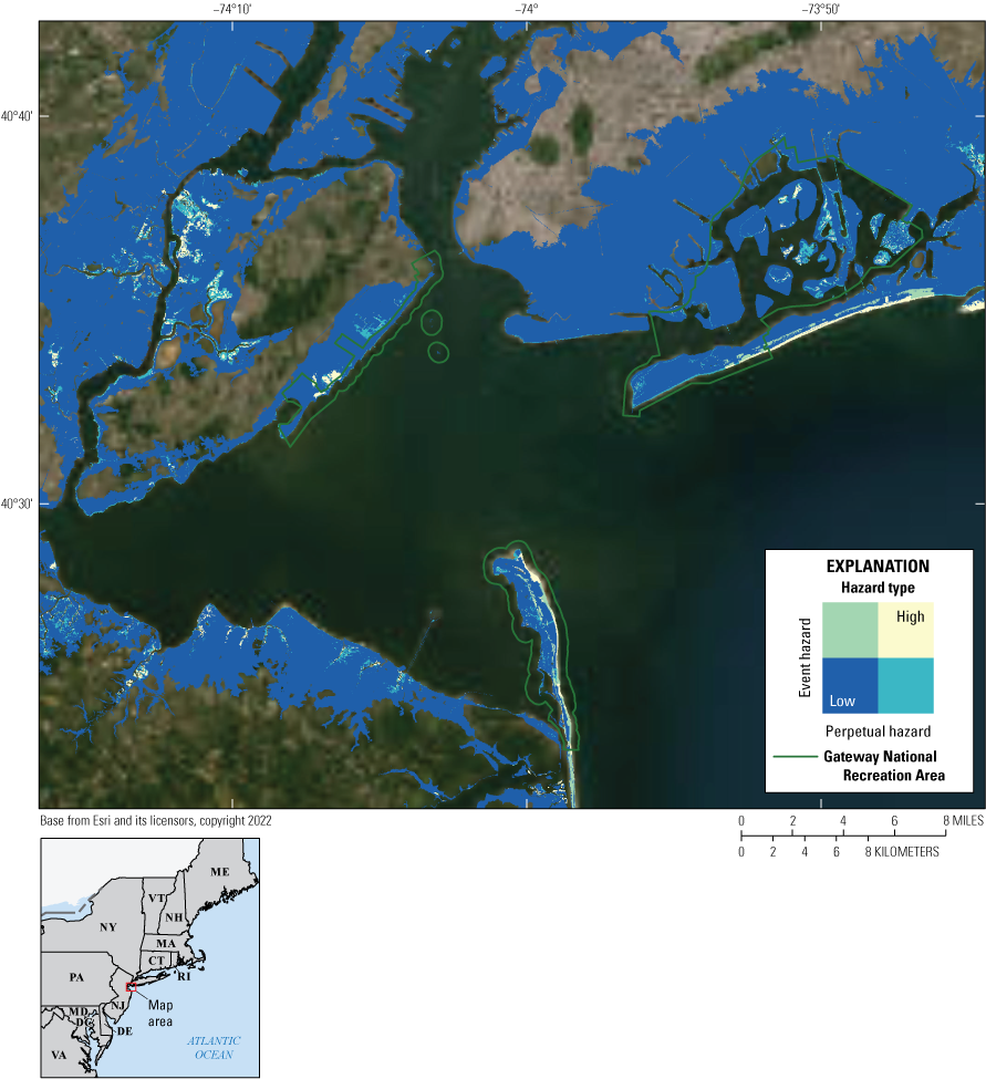
Map showing coastal change likelihood in Gateway National Recreation Area in New York and New Jersey, as part of the pilot study of the methodology of a coastal change likelihood assessment. The layer shows the hazards type (event or perpetual) that may be most influential to coastal change based on the comparison between the event and perpetual support vector machine output.
Datum
Vertical coordinate information is referenced to North American Vertical Datum of 1988 (NAVD 88) or Mean High Water (MHW) level.
Horizontal coordinate information is referenced to the World Geodetic System of 1984 (WGS 1984). Elevation, as used in this report, refers to distance above the vertical datum.
Abbreviations
C–CAP
Coastal Change Analysis Program
CCL
coastal change likelihood
CONED
Coastal National Elevation Database
CVI
coastal vulnerability index
DEM
digital elevation model
FWS
U.S. Fish and Wildlife Service
IPCC
Intergovernmental Panel on Climate Change
MHW
mean high water
NOAA
National Oceanic and Atmospheric Administration
NWI
National Wetland Inventory
USGS
U.S. Geological Survey
UVVR
unvegetated-to-vegetated ratio
Suggested Citation
Pendleton, E.A., Lentz, E.E., Sterne, T.K., and Henderson, R.E., 2023, Development and application of a coastal change likelihood assessment for the northeast region, Maine to Virginia: U.S. Geological Survey Data Report 1169, 56 p., https://doi.org/10.3133/dr1169.
ISSN: 2771-9448 (online)
Study Area
| Publication type | Report |
|---|---|
| Publication Subtype | USGS Numbered Series |
| Title | Development and application of a coastal change likelihood assessment for the northeast region, Maine to Virginia |
| Series title | Data Report |
| Series number | 1169 |
| DOI | 10.3133/dr1169 |
| Year Published | 2023 |
| Language | English |
| Publisher | U.S. Geological Survey |
| Publisher location | Reston, VA |
| Contributing office(s) | Woods Hole Coastal and Marine Science Center |
| Description | Report: viii, 56 p.; Data Release |
| Country | United States |
| State | Connecticut, Delaware, Maine, Maryland, Massachusetts, New Hampshire, New Jersey, New York, Rhode Island, Virginia |
| Online Only (Y/N) | Y |
| Additional Online Files (Y/N) | N |
| Google Analytic Metrics | Metrics page |