

A User Guide to Selecting Invasive Annual Grass Spatial Products for the Western United States
Links
- Document: Report (936 kB pdf) , HTML , XML
- Related Works:
- Data Report 1152 Compendium to Invasive Annual Grass Spatial Products for the Western United States, January 2010–February 2021
- Rangeland Ecology and Management Bridging the gap between spatial modeling and management of invasive annual grasses in the imperiled sagebrush biome
- Data Release: USGS Data Release— Database of invasive annual grass spatial products for the western United States January 2010 to February 2021
- Download citation as: RIS | Dublin Core
Background
Invasive annual grasses (IAGs)—including Bromus tectorum (cheatgrass), Taeniatherum caput-medusae (medusahead), and Ventenata dubia (ventenata) species—present significant challenges for rangeland management by altering plant communities, impacting ecosystem function, reducing forage for wildlife and livestock, and increasing fire risk (D’Antonio and Vitousek, 1992). Numerous spatial data products are used to map IAGs, and understanding the similarities, differences, and potential tradeoffs among these products is key to selecting the right maps for specific applications (Vaz and others, 2018; Sofaer and others, 2019). This short guide outlines considerations for selecting regional- and national-scale spatial data to support the management of IAGs.
Spatial Data Basics
Maps are generally developed based on remotely sensed inputs, including satellite or aerial photos, which are measured over time (fig. 1A). These are paired with field measurements of IAGs and other data, such as elevation, to create a model that predicts a map of IAGs (fig. 1B; Vaz and others, 2018; Funk and others, 2020). Several factors make this challenging, including variation in IAG cover over time owing to precipitation and fire, low percent cover within map pixels where IAGs occur, and confusion of IAGs with other vegetation (Smith and others, 2019). Some models combine data from multiple years to reduce error (fig. 1C; Rocchini and others, 2015), though this sacrifices some information about the current landscape and its changes over time (Funk and others, 2020). Models that do not use remote sensing data generally map only the potential for invasion. All models contain errors that result in imperfect maps; however, several kinds of evaluation metrics can be used to assess the level of confidence in map accuracy (Uden and others, 2015). Aerial imagery, such as that freely available on Google Earth and other web-based maps, and local monitoring information can be used together with map data to reduce uncertainty (Vaz and others, 2018). Knowing how best to use imperfect data is essential to their successful application (Sofaer and others, 2019).
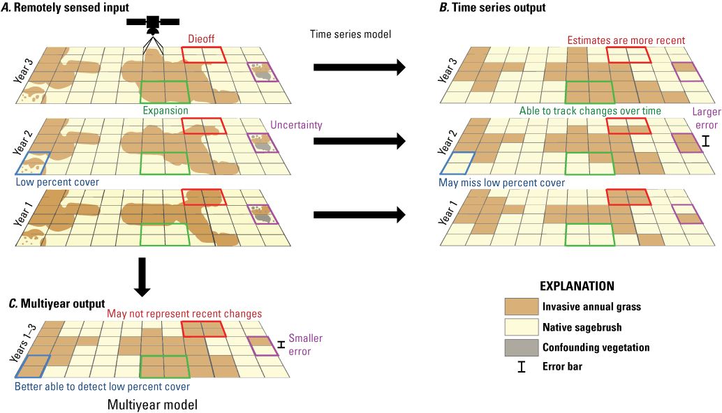
A, Example of invasive annual grass (IAG) spatial model development using remote sensing. B, A spatial map showing variability in IAG distribution over time, but which has inconsistent characterization of the right-most area resulting in larger error. C, A multiyear map of maximum or average IAG cover over a timeframe, which does not show variability over time but has smaller error. Colored outlines refer to IAG expansion (green), IAG dieoff (red), low IAG cover (blue), and uncertainty in IAG cover (purple).
U.S. Geological Survey Resources for Comparing and Selecting Spatial Data
For over 20 spatial data products representing annual grasses in the western United States published since 2010, refer to the following resources:
Product database.—Compares spatial data product attributes in a sortable, filterable spreadsheet: https://doi.org/10.5066/P9VW97AO.
Product compendium.—Includes 2-page spatial product summaries with key attributes, comparison tables, and web resources: https://doi.org/10.3133/dr20221152.
Journal article.—A review bridging science, spatial data, and action to manage invasive annual grasses: https://doi.org/10.1016/j.rama.2022.01.006.
Considerations for Selecting Spatial Data
The choice of IAG spatial products is not always easy. Consider these seven key criteria in the order listed when selecting maps for IAG management.
A. Geographic Extent
Determine if your geographic area is fully covered in the IAG map, which can sometimes be time consuming. Refer to our IAG product compendium for at-a-glance lists of States and thumbnails depicting the geographic extent of each map product. More detailed information, such as the range of latitude and longitude coordinates the product covers, can be found in our detailed product database.
B. Type of Map Outputs
Different map outputs and data types are better suited for different IAG management objectives. Spatial data describing species occurrence (presence or absence) are suitable for identifying areas where invasion has already occurred. Maps of habitat suitability predict the potential for invasion. Abundance metrics like percent cover or total biomass describe the intensity of invasion and are useful for targeting actions designed for early or fully established invasions (He and others, 2015). Many regional-scale map products do not distinguish among different species of annual grasses.
C. Spatial Resolution
Higher-resolution maps provide estimates of IAGs using smaller pixels (for example, 30×30 meters). A 30-m map will have 9 pixels for every pixel in a 90-m map. If accurate, higher-resolution maps can allow you to distinguish fine-scale differences in IAG occurrence or cover across the landscape. High resolution does not necessarily mean high accuracy: resolution describes the scale at which the map tries to distinguish pixels, and accuracy describes how well the map actually does this.
D. Recentness
The distribution and cover of IAGs are dynamic and highly variable within the growing season and across years. The timeframe represented in the map can affect interpretation and confidence in using the map for management applications. Recent data may provide a better snapshot of recent change than an older product. Time-series maps can estimate IAG expansion and contraction over time. Products that combine several years of data to create one map may better map areas with persistent IAG infestation, but they may not highlight recent changes (fig. 1; Rocchini and others, 2015).
E. Recommended Use and Caveats
Developers of IAG maps often indicate how their products are intended to be used and note key limitations. To ensure map data are used appropriately, users should consider whether their management needs align with the developer’s recommendations and examples of the product being used for similar purposes. Our product compendium and product database describe any recommendations and caveats stated by the authors of each map product.
F. Evaluation of Accuracy
Accuracy describes how well the map’s estimated locations and percent cover for IAGs represents the actual locations and percent cover on the ground. Although technically complex, a basic understanding of how spatial data products are evaluated is important when comparing and selecting products. A diversity of methods and metrics with varying statistical rigor are used to evaluate accuracy of products (Liu and others, 2009). Refer to “Evaluating the Accuracy of Spatial Products” for more details.
G. Model Approach and Inputs
When making a final decision on a map product, it is best to look at the technical details of the model approach. The relevance and quality of model inputs (for example, aerial or satellite imagery or field measurements) can influence model limitations and applications (Sofaer and others, 2019). Ideally, inputs represent the full range of environmental conditions that exist in the area of interest (He and others, 2015). Models that use dated inputs or exclude some environmental predictors of where IAGs occur may limit how maps can be interpreted and used to support management activities (Uden and others, 2015; Sofaer and others, 2019).
Selecting a Final Product
Narrow down the full set of map products to five or fewer that might meet your needs by assessing basic information (considerations A–D above). Then, move towards your final selection by considering the complex details in depth (steps 1–2). Finally, assess the product’s overall applicability by visualizing it with other information (steps 3–5).
Step 1—Compare and Contrast the Details
Learn how each product was developed and applied (considerations E and F), then scrutinize the details important for your application. Our product database characterizes more than 40 attributes for each product that we reviewed, and our product compendium provides simplified comparison tables and 2-page summaries.
Step 2—Compare Model Evaluation Results
Most models provide an accuracy score for model predictions (consideration F), but comparisons among products can be challenging owing to the variety of evaluation methods and metrics used. Accuracy scores themselves may have inaccuracy. Products with moderate accuracy scores estimated with more rigorous tests (for example, evaluated with fully independent data) may be as good as products with high accuracy scores estimated with less rigorous methods (for example, evaluated with nonindependent data). Tests that included data from your region of interest (consideration G) may yield higher confidence in the accuracy score than tests that did not (Smith and others, 2019). See “Evaluating the Accuracy of Spatial Products” for a detailed guide to accuracy.
Step 3—Examine the Map Product within Your Management Area
Overlay IAG maps with other data (for example, IAG point locations, maps of other landscape features) and evaluate the completeness of coverage. Use complementary vegetation maps and high-resolution aerial imagery to assess the degree of agreement among data. Individually, all such information will be incomplete and have limitations (Rocchini and others, 2015; Smith and others, 2019), but together these other data types can indicate areas of higher or lower confidence in IAG maps.
Step 4—Pair the Map Product with Local Information
Local information (for example, field and monitoring data) and field knowledge can help identify how well map products represent on-the-ground conditions. Regional map data are general characterizations of IAGs and should not always be expected to map small locations with high accuracy. Incorporating local information can help identify and account for discrepancies between regional and local patterns. Pairing IAG maps with high-resolution aerial imagery (fig. 2), field data, and local knowledge can help guide the appropriate use of regional spatial products for local applications (Sofaer and others, 2019).
Step 5—Reassess Limitations
To resolve questions about the limitations of IAG spatial data, consider reading the original documentation or contacting the map developer. Use-case examples can also provide insight into common applications and highlight potential limitations.

Prediction of invasive annual grass (IAG) distribution (left; from Dahal and others [2020], https://doi.org/10.5066/P9537QG9) can be paired with high-resolution aerial imagery (right) to spot check the accuracy of map products and identify areas in need of field surveys. IAGs appear as splotches of light green in early spring, which turn grayish green by summer (pictured). Native vegetation’s appearance (light tan in this example) will vary locally. Some native grasses can be difficult to distinguish from IAGs, but shrubs and trees are visible as individual plants.
Evaluating the Accuracy of Spatial Products
Accuracy evaluation is a complex topic, and a rigorous comparison requires more than simply determining whether one product's accuracy score is higher than another product’s accuracy score. It is important to examine whether and how the scoring measures can be compared and what dataset was used to estimate them.
Types of Measures
Many different accuracy measures are used to evaluate IAG models (Liu and others, 2009). Accuracy measures differ between products that map continuous outputs (for example, percent cover) and those that map categorical outputs (for example, occurrence; table 1). Accuracy may vary locally, but metrics are often reported only for the mapped area overall (Rocchini and others, 2015). For categorical maps, models estimate continuous probabilities, and a threshold cutoff is often selected to classify the landscape (for example, greater than 90-percent probability of presence yields “presence”). These accuracy measures report the prediction’s success dependent on the chosen threshold. Models are designed to optimize accuracy, but they do so in different ways. Some measures focus on correct prediction of actual IAG presence (optimizing true positives or false negatives) because these are relevant to early detection of invasion (Uden and others, 2015). Some models are designed to avoid overpredicting IAG where it is really absent (optimizing true negatives and false positives; Sofaer and others, 2019).
Rigor of Evaluation Dataset
Evaluations using independent data are more rigorous than those that reuse model building data for validation (Sofaer and others, 2019). Within-sample metrics compare model-building data to values predicted by the model and can overestimate accuracy. Cross-validation or bootstrapping uses all data to fit the final published model, but it assesses accuracy by refitting the model just to subsets of the data and seeing how well those models can predict other subsets of the data that are held out from fitting. This approach is less likely to overestimate accuracy. Fully independent evaluations compare model predictions to data never used in model building and are the most rigorous test type.
Table 1.
Overview of common accuracy measures, including the range of values observed in the IAG products reviewed in our product database.[All measures listed could be applied to either within-sample or fully independent data. IAG, invasive annual grass; %, percent; R2, coefficient of determination; MAE, mean of absolute error; RMSE, root mean squared error; nMAE, normalized mean of absolute error; nRMSE, normalized root mean squared error; >, greater than; <, less than; PCC, percent correctly classified; ROC, receiver operating characteristic; AUC, area under the curve; AUC-ROC, area under the curve receiver operating characteristic; AUPRC, area under the precision recall curve]
Assessing Tradeoffs in Product Choice
More than one spatial product may be suitable for an intended application, with potential tradeoffs (Sofaer and others, 2019). This section provides an example of such considerations using two hypothetical IAG maps for two applications: early detection and rapid response (table 2), and wildlife habitat assessments (table 3).
Table 2.
Example application of early detection and rapid response (for example, herbicide application) for cheatgrass invasion.[IAG, invasive annual grass; R2, coefficient of determination; AUC, area under the curve; %, percent]
| Consideration | Product A | Product B | Tradeoffs for application |
|---|---|---|---|
| Product type | Percent-cover map | Presence-absence map | The percent-cover map of product A may provide information on low to moderate percent cover of invasion in areas that could be targeted for herbicide application (for example, areas representing early infestation; Uden and others, 2015). The presence-absence map of product B lacks abundance information but may be suitable for identifying areas for additional early-detection surveys and rapid response. Adding a product that maps habitat suitability (not provided in this example) can also help identify watch list areas at high risk of invasion. |
| Species | IAGs (any species) | Cheatgrass | Both products are suitable if manager does not need species-specific information. If product B can reliably distinguish cheatgrass from other IAGs, it may provide species-specific information, but may include other IAGs as cheatgrass if discrimination is limited. |
| Spatial extent | Desert ecoregions of the western U.S.A. | Entirety of western U.S.A. | Both products cover the smaller extent. Examining the model details and evaluation may help determine whether the smaller-extent model, with spatially constrained environmental inputs, better represents IAGs than the larger-extent model representing a wider range of environmental conditions (Uden and others, 2015). If model inputs are tailored to a specific region, they may better reflect IAGs in that region but only if accuracy is also high. Regional products may perform well or poorly, depending on how well the smaller extent is represented in the larger model. |
| Spatial resolution | 30 meters | 250 meters | Product A supports spatial targeting of treatment areas using higher-resolution maps. Higher spatial resolution can more accurately map smaller patches of IAGs, but not necessarily. Examine for tradeoffs between resolution and accuracy (see “Evaluation accuracy”). |
| Recentness | Single map of average condition, 2016–2020 | Annual maps that create a time series, 1990–2016 | The composite map of product A can highlight recent IAG infestations and may better map all the areas suitable for the species by accounting for annual variation in IAG patches owing to weather. The time series of annual maps can be used to map where IAGs are changing through time, such as invasion fronts, but product B does not characterize recent coverage of IAGs. |
| Model inputs | Spectral imagery, topography, soil, climate, vegetation | Spectral imagery, topography, climate | Additional input variables may increase local accuracy of product A, but not necessarily, since some models with very few variables have high accuracy. Note that overreliance on indirect predictors like topography can reduce model performance (Uden and others, 2015). Models assessing large areas tend to place more emphasis on climatic covariates, which can be problematic in the context of climate change (He and others, 2015; Uden and others, 2015). |
| Evaluation of accuracy | Within sample R2 = 0.71 | Cross-validation sample AUC = 0.91 | Because product A is a continuous variable and product B is a categorical variable, they use different accuracy measures that cannot be directly compared. Product A’s R2 indicates good accuracy (71% of the variability in IAG percent cover is explained by their model) but it is based on within-sample validation which is less rigorous and likely to overestimate accuracy. Product B’s cross-validation sample is more rigorous, and 0.91 AUC value gives it an outstanding accuracy rating, but users should check region-specific accuracy (if possible). |
Table 3.
Example application of assessing wildlife habitat degradation by cheatgrass and other invasive annual grasses.[IAG, invasive annual grass; R2, coefficient of determination; AUC, area under the curve]
| Consideration | Product A | Product B | Tradeoffs for application |
|---|---|---|---|
| Product type | Percent cover map | Presence-absence map | Both products are suitable to assess areas affected by IAGs at some scale. Percent cover (product A) may better represent level of habitat degradation at a local or patch scale. Presence or absence (product B) can show habitat degradation at a landscape scale. |
| Species | IAGs (any species) | Cheatgrass | The species-level maps may not be needed if the wildlife species of interest responds similarly to different IAG species and management options are similar among IAGs. |
| Spatial extent | Desert ecoregions of the western U.S.A. | Entirety of western U.S.A. | Broader-extent maps may support comparisons of IAG threats across the full extent of the wildlife species’ range, whereas ecoregion-specific maps may not cover the species’ range. |
| Spatial resolution | 30 meters | 250 meters | If the wildlife species selects habitat and responds to habitat degradation at scales generally greater than 250 meters, both resolutions should represent the scale of habitat selection well. If it is a small-bodied species that selects at fine spatial scales, product A may be more suitable. |
| Recentness | Single map of average condition, 2016–20 | Annual maps that create a time series, 1990–2016 | The more recent years (2016–2020) of product A describe current coverage, and the multiyear composite may better capture the full range of climatic conditions that can support IAG in different years. The time series (product B) could be useful to assess long-term trends in habitat degradation and support assessments that link IAGs with population change. |
| Model inputs | Spectral imagery, topography, soil climate, vegetation | Spectral imagery, topography, climate | Additional input variables may increase local accuracy of product A, but not necessarily. Fewer input variables could increase the generality of the IAG map, allowing extrapolation and comparison across the full extent of wildlife habitat. |
| Evaluation of accuracy | Within sample R2 = 0.71 | Cross-validation sample AUC = 0.91 | See discussion in table 2. Product A is acceptable but has a less rigorous accuracy rating. Product B has outstanding accuracy and increases confidence in the map. Check to see if the product was evaluated using data from your region, as error can vary spatially. |
References Cited
Dahal, D., Wylie, B.K., Parajuli, S., and Pastick, N.J., 2020, Fractional estimates of invasive annual grass cover in dryland ecosystems of western United States (2016–2018): U.S. Geological Survey data release, accessed April 5, 2021, at https://doi.org/10.5066/P9537QG9.
D’Antonio, C.M., and Vitousek, P.M., 1992, Biological invasions by exotic grasses, the grass/fire cycle, and global change: Annual Review of Ecology and Systematics, v. 23, no. 1, p. 63–87. [Also available at https://doi.org/10.1146/annurev.es.23.110192.000431.]
Funk, J.L., Parker, I.M., Matzek, V., Flory, S.L., Aschehoug, E.T., D’Antonio, C.M., Dawson, W., Thomson, D.M., and Valliere, J., 2020, Keys to enhancing the value of invasion ecology research for management: Biological Invasions, v. 22, no. 8, p. 2431–2445. [Also available at https://doi.org/10.1007/s10530-020-02267-9.]
He, K.S., Bradley, B.A., Cord, A.F., Rocchini, D., Tuanmu, M.-N., Schmidtlein, S., Turner, W., Wegmann, M., and Pettorelli, N., 2015, Will remote sensing shape the next generation of species distribution models?: Remote Sensing in Ecology and Conservation, v. 1, no. 1, p. 4–18. [Also available at https://doi.org/10.1002/rse2.7.]
Liu, C., White, M., and Newell, G., 2009, Measuring the accuracy of species distribution models—A review, in Anderssen, R.S., Braddock, R.D., and Newham, L.T.H., eds., Proceedings of the 18th World IMACs/MODSIM Congress, Cairns, Australia, July 13–17, 2009: International Association for Mathematics and Computers in Simulation and Modelling and Simulation Society of Australia and New Zealand, p. 4241–4247.
Rocchini, D., Andreo, V., Förster, M., Garzon-Lopez, C.X., Gutierrez, A.P., Gillespie, T.W., Hauffe, H.C., He, K.S., Kleinschmit, B., Mairota, P., Marcantonio, M., Metz, M., Nagendra, H., Pareeth, S., Ponti, L., Ricotta, C., Rizzoli, A., Schaab, G., Zebisch, M., Zorer, R., and Neteler, M., 2015, Potential of remote sensing to predict species invasions: Progress in Physical Geography, v. 39, no. 3, p. 283–309. [Also available at https://doi.org/10.1177/0309133315574659.]
Smith, W.K., Dannenberg, M.P., Yan, D., Herrmann, S., Barnes, M.L., Barron-Gafford, G.A., Biederman, J.A., Ferrenberg, S., Fox, A.M., Hudson, A., Knowles, J.F., MacBean, N., Moore, D.J.P., Nagler, P.L., Reed, S.C., Rutherford, W.A., Scott, R.L., Wang, X., and Yang, J., 2019, Remote sensing of dryland ecosystem structure and function—Progress, challenges, and opportunities: Remote Sensing of Environment, v. 233, p. 111401. [Also available at https://doi.org/10.1016/j.rse.2019.111401.]
Sofaer, H.R., Jarnevich, C.S., Pearse, I.S., Smyth, R.L., Auer, S., Cook, G.L., Edwards, T.C., Jr., Guala, G.F., Howard, T.G., Morisette, J.T., and Hamilton, H., 2019, Development and delivery of species distribution models to inform decision-making: Bioscience, v. 69, no. 7, p. 544–557. [Also available at https://doi.org/10.1093/biosci/biz045.]
Uden, D.R., Allen, C.R., Angeler, D.G., Corral, L., and Fricke, K.A., 2015, Adaptive invasive species distribution models—A framework for modeling incipient invasions: Biological Invasions, v. 17, no. 10, p. 2831–2850. [Also available at https://doi.org/10.1007/s10530-015-0914-3.]
Vaz, A.S., Alcaraz-Segura, D., Campos, J.C., Vicente, J.R., and Honrado, J.P., 2018, Managing plant invasions through the lens of remote sensing—A review of progress and the way forward: The Science of the Total Environment, v. 642, p. 1328–1339. [Also available at https://doi.org/10.1016/j.scitotenv.2018.06.134.]
Suggested Citation
Van Schmidt, N.D., Shyvers, J.E., Saher, D.J., Tarbox, B.C., Heinrichs, J.A., and Aldridge, C.L., 2022, A user guide to selecting invasive annual grass spatial products for the western United States: U.S. Geological Survey Fact Sheet 2022-3001, 6 p., https://doi.org/10.3133/fs20223001.
ISSN: 2327-6932 (online)
Study Area
| Publication type | Report |
|---|---|
| Publication Subtype | USGS Numbered Series |
| Title | A user guide to selecting invasive annual grass spatial products for the western United States |
| Series title | Fact Sheet |
| Series number | 2022-3001 |
| DOI | 10.3133/fs20223001 |
| Year Published | 2022 |
| Language | English |
| Publisher | U.S. Geological Survey |
| Publisher location | Reston, VA |
| Contributing office(s) | Fort Collins Science Center |
| Description | Fact Sheet: 6 p.; Data Release |
| Country | United States |
| Other Geospatial | western United States |
| Google Analytic Metrics | Metrics page |