

Documentation of Models Describing Relations Between Continuous Real-Time and Discrete Water-Quality Constituents in the Little Arkansas River, South-Central Kansas, 1998–2019
Links
- Document: Report (1.82 MB pdf) , HTML , XML
- Appendixes:
- Appendix 1 (zip) —Model Archive Summaries for the Little Arkansas River at Highway 50 near Halstead, Kansas (Halstead Site; U.S. Geological Survey Station Number 07143672)
- Appendix 2 (zip) —Model Archive Summaries for the Little Arkansas River near Sedgwick, Kansas (Sedgwick Site; U.S. Geological Survey Station Number 07144100)
- Dataset: USGS National Water Information System database —USGS water data for the Nation
- Download citation as: RIS | Dublin Core
Acknowledgments
The authors thank Shawn Maloney and Scott Macey of the City of Wichita for technical assistance. The authors appreciate the assistance of Vernon Strasser and the laboratory staff at the City of Wichita Municipal Water and Wastewater Laboratory for providing a substantial proportion of the chemical analyses used for model development.
The authors thank the U.S. Geological Survey staff that assisted with data collection, analysis, and interpretation, including Trudy Bennett, Barbara Dague, Carlen Collins, John Rosendale, David Eason, Patrick Eslick, and Diana Restrepo-Osorio. The authors also thank U.S. Geological Survey technical reviewers Kyle Juracek, Patrick Eslick-Huff, and Dale Robertson.
Abstract
Data were collected at two monitoring sites along the Little Arkansas River in south-central Kansas that bracket most of the easternmost part of the Equus Beds aquifer. The data were used as part of the city of Wichita’s aquifer storage and recovery project to evaluate source water quality. The U.S. Geological Survey, in cooperation with the City of Wichita, has continued to monitor the water quality of these sites through 2019 to update previously published regression-based models using continuously measured physicochemical properties and discretely sampled water-quality constituents of interest. The purpose of this report is to provide an update of the previously published linear regression models that have been used to continuously compute estimates of water-quality constituent concentrations or densities at these two sites. Water-quality constituent model updates include those for dissolved and suspended solids, suspended-sediment concentration, hardness, alkalinity, primary ions (bicarbonate, calcium, sodium, chloride, and sulfate), nutrients (total Kjeldahl nitrogen and total phosphorus), total organic carbon, indicator bacteria (Escherichia coli and fecal coliform bacteria), a trace element (arsenic), and a pesticide (atrazine).
Regression analyses were used to develop surrogate models that related continuously measured physicochemical properties, streamflow, and seasonal components to discretely sampled water-quality constituent concentrations or densities. Specific conductance was an explanatory variable for dissolved solids, primary ions, and atrazine. Turbidity was an explanatory variable for total suspended solids and sediment, nutrients, total organic carbon, and indicator bacteria. Streamflow and water temperature were explanatory variables for dissolved arsenic. Seasonal components were included as explanatory variables for atrazine models. The amount of variance explained by most of the updated models was within 5 percent of previously published models.
Introduction
The water supply of the city of Wichita in south-central Kansas comes from two primary sources—the Equus Beds aquifer and Cheney Reservoir (fig. 1). Historically, the volume of water pumped out of parts of the Equus Beds aquifer exceeded the natural recharge rate and aquifer water levels have decreased (Hansen and others, 2014; Whisnant and others, 2015; Klager, 2016). The easternmost area of the aquifer that includes the Wichita well field (fig. 1) is susceptible to saltwater contamination from the Arkansas River (fig. 1) and saltwater intrusion from the oil field evaporation pit contamination plumes created in the 1930s (Whittemore, 2007; Klager and others, 2014). The Equus Beds aquifer storage and recovery project was created to help Wichita meet increasing water demands and, as an added benefit, inhibit saltwater encroachment (Ziegler and others, 2010; Klager and others, 2014). Source water for artificial recharge is obtained from the Little Arkansas River (fig. 1) and is injected into the Equus Beds aquifer for later use.
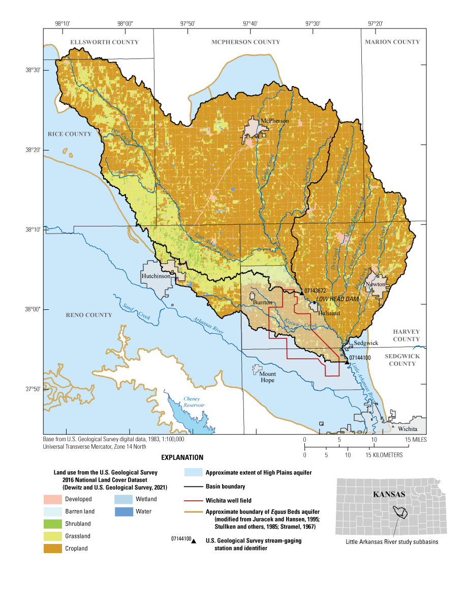
Study area location in the Little Arkansas River drainage basin in south-central Kansas and its land use categories.
The sites Little Arkansas River at Highway 50 near Halstead, Kansas (hereafter referred to as the “Halstead site,” U.S. Geological Survey [USGS] station 07143672, fig. 1) and Little Arkansas River near Sedgwick, Kansas (hereafter referred to as the “Sedgwick site,” USGS station 07144100, fig. 1) bracket most of the easternmost part of the Equus Beds aquifer. Data were collected for these two sites as part of the aquifer storage and recovery project to evaluate source water quality. Real-time water-quality monitors were installed to provide continuous measures of water temperature, specific conductance, pH, dissolved oxygen, turbidity, nitrate plus nitrite, and colored dissolved organic matter fluorescence (fDOM). Continuous measurement of water-quality physicochemical properties in near real time allowed characterization of surface water during conditions in the Little Arkansas River at time scales that would not have been possible otherwise and serves as a complement to discrete water-quality sampling. Regression models based on surrogate water-quality measurements in real time are useful to compute estimates of continuous water-quality constituent concentrations to support water treatment and recharge decisions, to compare to water-quality criteria, and to compute loads and yield to assess drainage basin transport. Physicochemical properties and water-quality constituents in the Little Arkansas River that may exceed Federal (U.S. Environmental Protection Agency, 2009) drinking water regulations or are of potential interest or concern for artificial recharge operations include streamflow, chloride, sulfate, nitrate plus nitrite, total coliform bacteria, iron (not addressed in this study), manganese (not addressed in this study), arsenic, and atrazine (Ziegler and others, 2010; Tappa and others, 2015; Stone and others, 2019).
Linear regression models for the Halstead and Sedgwick sites were developed from relations between continuously measured physicochemical properties and discretely sampled water-quality constituents. The models were published by Christensen and others (2003) and Rasmussen and others (2016) as part of monitoring aquifer storage and recovery source water efforts. The USGS, in cooperation with the City of Wichita, has continued water-quality monitoring, in part, to update the previously published regression-based models developed by Rasmussen and others (2016) using continuously measured physicochemical properties and discretely sampled water-quality constituents of interest during 1998 through 2019.
Purpose and Scope
The purpose of this report is to provide an update of previously published regression models (Rasmussen and others, 2016) that have been used to continuously compute estimates of water-quality constituent concentrations or densities at the Halstead and Sedgwick sites along the Little Arkansas River in south-central Kansas. Water-quality constituent model updates include those for dissolved and suspended solids, suspended-sediment concentration, hardness, alkalinity, primary ions (bicarbonate, calcium, sodium, chloride, and sulfate), nutrients (total Kjeldahl nitrogen and total phosphorus), total organic carbon, indicator bacteria (Escherichia coli [E. coli] and fecal coliform bacteria), a trace element (arsenic), and a pesticide (atrazine). Site-specific regression models were updated to provide real-time information to the city of Wichita to adjust water treatment and to provide water-quality information for source water used for recharge. Real-time computations of water-quality concentrations are available at the USGS National Real-Time Water-Quality website (https://nrtwq.usgs.gov). The water-quality information in this report allows the concentrations or densities of many potential constituents of concern, including chloride, nutrients, sediment, bacteria, and atrazine to be estimated in real time and characterized during conditions and time scales that would not be possible otherwise. Additionally, the methods and techniques in this study can be applied to other sites regionally, nationally, and globally.
Description of Study Area
The study area is in south-central Kansas (fig. 1). The Halstead and Sedgwick sites are USGS stations on the Little Arkansas River near Halstead and Sedgwick, Kansas, respectively. The Little Arkansas River has a contributing drainage area of 1,266 square miles (Albert and Stramel, 1966) of primarily agricultural land that produces corn, sorghum, soybeans, and wheat. The Halstead site has a contributing drainage area of 685 square miles, and the Sedgwick site has a contributing drainage area of 1,165 square miles (U.S. Geological Survey, 2021). Streamflow at both sites is affected by groundwater withdrawals, surface-water diversions, and return flow from irrigated areas. In the study area, long-term mean annual precipitation (1900 through 2019), based on data recorded near Mount Hope, Kansas (fig. 1; National Oceanic and Atmospheric Administration, 2020), was 30.2 inches (table 1). During the study period (1998 through 2019), mean annual precipitation was 33.7 inches (table 1).
Table 1.
Annual total and mean-annual precipitation during 1998 through 2019 and mean-annual precipitation during 1900 through 2019 at the “MT HOPE” (Global Historical Climatology Network–Daily:USC00145539) station.[Data are from National Oceanic and Atmospheric Administration (2020)]
The Kansas Department of Health and Environment has listed several streams in the Little Arkansas River drainage basin as impaired waterways under section 303(d) of the 1972 Clean Water Act (Kansas Department of Health and Environment, 2020). Impairments for streams in or near the study area include arsenic and chloride for water supply; dissolved oxygen, selenium, total suspended solids, atrazine, copper, total phosphorus, biology (nutrients and oxygen demand impact on aquatic life), and sediment for aquatic life; and E. coli bacteria for recreation (Kansas Department of Health and Environment, 2020). Main pollutants of concern listed in the Little Arkansas River Watershed Restoration and Protection Strategy were atrazine, sediment, nutrients, and fecal coliform bacteria (Kansas State University Research and Extension and others, 2011). The Little Arkansas River has defined total maximum daily loads for atrazine (Kansas Department of Health and Environment, 2008), nutrients and oxygen demand (Kansas Department of Health and Environment, 2000b), sediment (Kansas Department of Health and Environment, 2000a), chloride (Kansas Department of Health and Environment, 2006a, 2006b), fecal coliform bacteria (Kansas Department of Health and Environment, 2000c), total suspended solids (Kansas Department of Health and Environment, 2014), and total phosphorus and pH (Kansas Department of Health and Environment, 2019).
Methods
Continuously measured physicochemical properties and seasonal components (also used as surrogates in regression relations) and discretely collected water-quality constituent data during January 1998 through December 2019 were used to update previously published site-specific linear regression models developed by Rasmussen and others (2016) for the Halstead and Sedgwick sites along the Little Arkansas River. Models were updated for dissolved and suspended solids, suspended-sediment concentration, hardness, alkalinity, primary ions (bicarbonate, calcium, sodium, chloride, and sulfate), nutrients (total Kjeldahl nitrogen and total phosphorus), total organic carbon, indicator bacteria (E. coli and fecal coliform bacteria), a trace element (arsenic), and a pesticide (atrazine). Additional streamflow-based (without other continuous surrogates, with the exception of seasonal components) models were developed to compute concentrations during periods when concomitant continuous water-quality data were unavailable.
Continuous Streamflow and Water-Quality Monitoring
Continuous (1-hour maximum interval) streamflow and water-quality physicochemical properties were measured at the Halstead and Sedgwick sites during the study period. Streamflow has been measured at the Halstead and Sedgwick sites since May 1995 and November 1993, respectively. Streamflow was measured using standard USGS methods (Sauer and Turnipseed, 2010; Turnipseed and Sauer, 2010; Painter and Loving, 2015). Water-quality physicochemical properties (continuous surrogates) used for model development in this report included water temperature, specific conductance, pH, dissolved oxygen, turbidity, nitrate plus nitrite, and fDOM.
Since June-October 1988, both sites have been equipped with a YSI Incorporated 6600 Extended Deployment System water-quality monitor (YSI Incorporated, 2012a) to continuously measure (60-minute interval) water temperature, specific conductance, pH, dissolved oxygen (YSI Clark cell or optical dissolved oxygen sensors), and turbidity (YSI 6026 or 6136 optical turbidity sensors). Detailed method descriptions for continuous water-quality monitoring by the USGS Kansas Water Science Center are in Bennett and others (2014). Nitrate sensors (HACH Nitratax plus sc; HACH Company, 2014) were installed at the Sedgwick site in March 2012 and the Halstead site in February 2017. Nitrate sensor data include nitrite and, therefore, are reported and referred to as nitrate plus nitrite concentrations (Pellerin and others, 2013) in this report. Surface-water monitors were installed near the centroid of the stream cross section to best represent stream width conditions and were maintained following standard USGS procedures (Wagner and others, 2006; Rasmussen and others, 2008; Pellerin and others, 2013; Bennett and others, 2014).
Some equipment was upgraded throughout the life of the project. YSI 6136 turbidity sensors were initially installed at both sites in July 2004. A Xylem YSI EXO2 water-quality monitor (YSI Incorporated, 2012b) equipped with water temperature, specific conductance, pH, dissolved oxygen, turbidity, and YSI EXO fDOM sensors was installed in September 2014 at the Sedgwick site and in January 2017 at the Halstead site. Because of differences in turbidity sensor readings between the YSI 6136 and YSI EXO turbidity sensors (Stone and others, 2019), only YSI EXO turbidity sensor data were used for model development in this report although turbidity data were available since June-October 1998. Continuous water-quality data for Kansas are available at the National Water Information System database (U.S. Geological Survey, 2021).
Discrete Water-Quality Data Collection
During 1998 through 2019, about eight discrete surface-water water-quality samples were collected annually at both study sites across a range of Little Arkansas River streamflow conditions using USGS equal-width increment methods (U.S. Geological Survey, 2006; Stone and others, 2012; Rasmussen and others, 2014; Stone and others, 2019). These samples were analyzed for dissolved (number of samples [n] at the Halstead site [Halstead n]=218 and n at the Sedgwick site [Sedgwick n]=345) and suspended solids (Halstead n=186 and Sedgwick n=234); suspended-sediment concentration (Halstead n=178 and Sedgwick n=315); hardness (Halstead n=218 and Sedgwick n=351); alkalinity (Halstead n=34 and Sedgwick n=147); primary ions (bicarbonate [Halstead n=34 and Sedgwick n=147]; calcium [Halstead n=217 and Sedgwick n=351]; sodium [Halstead n=217 and Sedgwick n=351]; chloride [Halstead n=219 and Sedgwick n=360]; and sulfate [Halstead n=217 and Sedgwick n=356]); nutrients (total Kjeldahl nitrogen [Halstead n=168 and Sedgwick n=304] and total phosphorus [Halstead n=168 and Sedgwick n=304]); total organic carbon (Halstead n=130 and Sedgwick n=167); indicator bacteria (E. coli [Halstead n=151 and Sedgwick n=183] and fecal coliform bacteria [Halstead n=216 and Sedgwick n=261]); arsenic (Halstead n=167 and Sedgwick n=312); and atrazine (Halstead n=176 and Sedgwick n=323). Collection and analyses for dissolved and total suspended solids, suspended-sediment concentration, primary ions, nutrients, total organic carbon, arsenic, bacteria, and pesticides followed methods described by Ziegler and Combs (1997), Ziegler and others (1999, 2010), Stone and others (2012, 2016, 2019), and Tappa and others (2015). Indicator bacteria analyses were done using methods described by the U.S. Environmental Protection Agency (2000, 2006a, 2006b) and Myers and others (2014).
Dissolved solids, primary ions, nutrients, total organic carbon, and arsenic samples were analyzed by the Wichita Municipal Water and Wastewater Laboratory and the USGS National Water Quality Laboratory (Denver, Colorado). Suspended-sediment concentrations were analyzed at the USGS Iowa Sediment Laboratory (Iowa City, Iowa) following methods described in Guy (1969). Indicator bacteria samples were analyzed by the USGS Kansas Water Science Center (Lawrence, Kansas). Atrazine was analyzed by the USGS National Water Quality Laboratory. Discrete water-quality data are available at the National Water Information System database (U.S. Geological Survey, 2021).
Quality Assurance and Quality Control
Quality-assurance and quality-control samples were collected routinely during the study period to identify, quantify, and document bias and variability in data resulting from collecting, processing, handling, and analyzing samples (U.S. Geological Survey, 2006). Relative percentage difference (RPD) was calculated to quantify differences in water-quality monitor measurements and discrete sample analyte concentrations detected in replicate water-quality samples. The RPD was calculated by dividing the difference between replicate pairs by the mean and multiplying that value by 100, resulting in a value representing the percentage difference between replicate samples (Zar, 1999).
Water temperature, specific conductance, pH, and dissolved oxygen sensor data did not exceed operational limits and the Xylem YSI EXO turbidity sensor did not exceed the maximum operational limit (4,000 formazin nephelometric units) during the study period. Time-series measurements were occasionally missing or deleted from the dataset because of equipment malfunction, excessive fouling caused by environmental conditions, extreme low- or no-flow conditions, or temporary removal of equipment because of ice. During the study period (January 1998 through December 2019), 3 and 4 percent of the hourly streamflow record, 6 and 3 percent of the water temperature record, 8 and 9 percent of the specific conductance record, 6 and 4 percent of the pH record, 8 and 6 percent of the dissolved oxygen record, 2 and 6 percent of the YSI EXO turbidity record, 4 and 7 percent of the fDOM record, and 1 and 11 percent of the nitrate plus nitrite record were missing or deleted (table 2) at the Halstead and Sedgwick sites, respectively. Most of the missing data were because of low flow or icy conditions and occasionally sensor fouling. The fDOM data were temperature and turbidity corrected following protocols described by Downing and others (2012).
Table 2.
Summary statistics for continuously (hourly) measured physicochemical properties for the Little Arkansas River at Highway 50 near Halstead, Kansas (Halstead site; U.S. Geological Survey station number 07143672), and Little Arkansas River near Sedgwick, Kansas (Sedgwick site; U.S. Geological Survey station number 07144100), during 1998 through 2019.[Continuous real-time water-quality data are available on the U.S. Geological Survey (USGS) National Real-Time Water-Quality website (https://nrtwq.usgs.gov/ks); n, number of measurements; pcode, parameter code; <, less than]
Data temperature and turbidity corrected following Downing and others (2012).
Comparison of field cross-sectional measurements collected during high- and low-flow conditions at the surface-water sites with the continuous data provided verification that bias in continuous data because of monitor location within the stream cross section was minimal. Median RPDs between continuous and field water-quality monitor measurements were less than (<) 2 percent, except for dissolved oxygen (<4 percent), Xylem YSI EXO sensor turbidity (<6 percent), and fDOM (<19 percent; table 3). The largest differences between continuous and field-monitor values commonly occurred when conditions were changing rapidly.
Table 3.
Summary of quality-control replicate and blank results for the Little Arkansas River at Highway 50 near Halstead, Kansas (Halstead site; U.S. Geological Survey station number 07143672), and Little Arkansas River near Sedgwick, Kansas (Sedgwick site; U.S. Geological Survey station number 07144100), during 1998 through 2019.[RPD, relative percentage difference; Min, minimum; Max, maximum; Med, median; °C, degree Celsius; pcode, U.S. Geological Survey parameter code; --, not applicable; µS/cm, microsiemen per centimeter at 25 degrees Celsius; mg/L, milligram per liter; FNU, formazin nephelometric unit; µg/L, microgram per liter; QSE, quinine sulfate equivalent; CaCO3, calcium carbonate; mpn/100 mL, most probable number per 100 milliliters; col/100 mL, colony per 100 milliliters]
About 10 percent of the discrete water-quality samples were quality-assurance and quality-control samples and included concurrent replicates, field and equipment blanks, and standard reference samples. Concurrent replicate samples were collected to quantify variability potentially introduced by sample collection, processing techniques, and analytical method (Bennett and others, 2014, Mueller and others, 2015). RPDs were not calculated for replicate pairs that had consistent nondetections (both values in the replicate pair were censored) or inconsistent detections (one value in the replicate pair was a detected value and the other value was censored; Mueller and others, 2015); these pair types occurred only in three indicator bacteria replicate pairs. Replicate comparisons included 86 dissolved and total suspended solids pairs, 34 suspended-sediment concentration pairs, 205 primary ion pairs, 70 nutrient pairs, 27 total organic carbon pairs, 68 indicator bacteria pairs (containing 1 inconsistent E. coli bacteria pair detection and 2 consistent fecal coliform bacteria pair nondetections), 32 dissolved arsenic pairs, and 25 atrazine pairs. Median dissolved solids, hardness, calcium, sodium, alkalinity, bicarbonate, chloride, sulfate, and total phosphorus RPDs were <2 percent; median total suspended solids, total Kjeldahl nitrogen, arsenic, atrazine, total organic carbon, and suspended sediment RPDs were <6 percent; median E. coli bacteria RPD was 8.8 percent; and median fecal coliform bacteria RPD was 20 percent (table 3). Largest RPD values generally occurred when the values were near the laboratory reporting level.
Blank samples consisted of deionized water, inorganic blank water, or organic blank water, depending on analyses. During the study period, 63 blank samples for modeled analytes were collected and analyzed for dissolved and suspended solids, hardness, calcium, sodium, chloride, sulfate, total Kjeldahl nitrogen, total phosphorus, total organic carbon, E. coli and fecal coliform bacteria, dissolved arsenic, and atrazine. Suspended solids, hardness, chloride, sulfate, total phosphorus, and arsenic blank samples did not have any detections during the study period. Blank samples with analyte detections included dissolved solids (four detections), calcium and sodium (three detections each), total Kjeldahl nitrogen (five detections), total organic carbon (six detections), E. coli and fecal coliform bacteria (one detection each), and atrazine (two detections table 3). Blank sample analyte detections were at or below either the analytical detection limit or minimum reporting limit except for one dissolved solids detection, one total Kjeldahl nitrogen detection, and one total organic carbon detection. Detection or minimum reporting limit exceedances were near the analytical detection or minimum reporting limit.
Standard reference samples were analyzed by the Wichita Municipal Water and Wastewater Laboratory and analytical results were submitted to the USGS Branch of Quality Systems annually and oftentimes biannually for laboratory-performance evaluation. Standard reference sample data are available at https://bqs.usgs.gov/srs. Most of the reported values were within 10 percent of the most probable value during the study. Median RPDs between laboratory results and most probable values indicated that laboratory data generally were consistent and unbiased.
Regression Model Development
Simple linear (ordinary least squares [OLS]) and Tobit regression analyses were used to develop regression models that related continuously measured physicochemical properties (continuous surrogates), streamflow, and seasonal components to discretely sampled water-quality constituent concentrations or densities (Rasmussen and others, 2009; Helsel and others, 2020). The previously published (Rasmussen and others, 2016) models for dissolved solids, suspended solids, suspended-sediment concentration, hardness, alkalinity, bicarbonate, calcium, sodium, chloride, sulfate, total Kjeldahl nitrogen, total phosphorus, total organic carbon, E. coli bacteria, fecal coliform bacteria, arsenic, and atrazine were updated following methods described in Rasmussen and others (2009, 2016). Additional streamflow-based models (with streamflow and seasonal components) were developed to compute estimates of concentrations or densities during periods when concomitant continuous surrogate measurements were unavailable.
Regression models were developed using OLS estimation for constituents that had datasets without left-censored data (< values). Tobit regression methods were used for fitting linear models for constituents that had datasets with left-censored data using absolute maximum likelihood estimation (AMLE; Hald, 1949; Cohen, 1950; Tobin, 1958; Helsel and others, 2020). Discrete datasets containing left-censored data included total suspended solids (5–8 percent left-censored data), chloride (<1–2 percent left censored data), sulfate (3–4 percent left-censored data), E. coli bacteria (1 percent left-censored data), fecal coliform bacteria (<1 percent left-censored data), dissolved arsenic (<1–2 percent left-censored data), and atrazine (1–3 percent left-censored data). Data and models for this report were analyzed and developed using R (version 4.0.0) programming language (R Core Team, 2020). Tobit regression models were developed using absolute maximum likelihood estimation methods using the smwrQW (v.0.7.9) package in R programming language (R Core Team, 2020).
Model datasets had different numbers of measurements for the following two primary reasons:
-
The sampling date ranges and frequencies of each discrete water-quality constituent were not always identical.
-
Available concomitant real-time data date ranges were not identical among data and sensor type—streamflow, water temperature, specific conductance, pH, and dissolved oxygen data were available during 1998 through 2019 (Halstead and Sedgwick sites); YSI EXO turbidity and fDOM data were available during 2014 through 2019 (Sedgwick site) and 2017 through 2019 (Halstead site); and nitrate plus nitrite data were available during 2017 through 2019 (Halstead and Sedgwick sites) (table 2).
Model datasets and modeled constituents included available concomitant real-time physicochemical properties as explanatory variables during model development. Potential explanatory variables were evaluated individually and in combination and included available concomitant continuously measured streamflow, water temperature, specific conductance, pH, dissolved oxygen, turbidity (YSI EXO turbidity sensor), fDOM, and nitrate plus nitrite concentration for the updated models. Periodic functions (seasonal components sine and cosine variables) also were evaluated as potential explanatory variables using day of the year. Explanatory variables were interpolated within the continuous record based on discrete sample time. The maximum time span between two continuous data points used for interpolation was 2 hours.
Potential linear regression models were evaluated based on diagnostic statistics (coefficient of determination [R2], or adjusted R2 for OLS-estimated models; pseudo-R2 for AMLE-estimated models; Mallow’s Cp for OLS-estimated models; root mean square error for OLS-estimated models; prediction error sum of squares for OLS-estimated models; and residual standard error for AMLE-estimated models), patterns in residual plots, and the range and distribution of discrete and continuous data (Helsel and others, 2020). Updated models were selected regardless of the date ranges of available concomitant real-time surrogate data (table 2) that
-
maximized response variable variance explained by the model (R2 or adjusted R2 for OLS-estimated models and pseudo-R2 for AMLE-estimated models),
-
maximized fit to the data (Mallow’s Cp for OLS-estimated models), and
-
minimized heteroscedasticity (irregular scatter) in residual plots and uncertainty associated with computed values (root mean square error and prediction error sum of squares for OLS-estimated models and residual standard error for AMLE-estimated models).
If either a sine or cosine seasonality variable was included in the model, a corresponding counterpart also was included in the model. A bias correction factor was calculated for models with logarithmically transformed response variables because transformation of estimates to original units results in a low biased estimate (Duan, 1983; Helsel and others, 2020).
Potential outliers were identified following Rasmussen and others (2009) and Helsel and others (2020). Studentized residuals, leverage, Cook’s D (Cook, 1977), and difference in fits values were used to identify influential data points for OLS-estimated models; and leverage and Cook’s D values were used to identify influential data points for AMLE-estimated models. Studentized residuals are used to identify outliers with high leverage, Cook’s D is a combination of each observation’s leverage and residual value (large values indicate influential observations), and difference in fits is the product of the Studentized residual and leverage (large values indicate influential observations). Removing data points that were based only on outlier criteria may only overestimate the certainty of the model. Data points that were not representative of the dataset and exceeded Cook’s D and difference in fits thresholds for OLS-estimated models and Cook’s D thresholds for AMLE-estimated models were removed from model datasets to avoid erroneous inflation of model-computed values at the upper range of surrogate relations.
Updated Regression Models
Previously published (Rasmussen and others, 2016) regression models were updated for the 17 water-quality constituents (solids and primary ions, nutrients, total organic carbon, indicator bacteria, a trace element, and a pesticide) for the Halstead and Sedgwick sites along the Little Arkansas River. Additional streamflow-based models were developed to compute estimates of constituents of interest when concomitant continuous data were unavailable to compute more complete load estimates. Additional models are not intended to stand alone, are not intended to be used under any other circumstance, and are not discussed further in this report; these additional models are the second model listed in tables 4, 5, 6, 7, and 8 for the updated Halstead and Sedgwick regression models. Regression model summaries are presented in appendixes 1 (Halstead site) and 2 (Sedgwick site). Model forms (independent and explanatory variables) and the amount of variance explained by the updated models were generally similar to the original models (Rasmussen and others, 2016; tables 4–8). Model forms (selected explanatory variables) for most updated models remained unchanged (tables 4–8). Continuously measured physicochemical properties that were included as surrogates in final models for this study were streamflow, water temperature, specific conductance, and turbidity (tables 4–8). Continuously measured physicochemical properties that were not selected as surrogates for the updated models in this report included pH, dissolved oxygen, nitrate plus nitrite, and fDOM (tables 4–8).
Table 4.
Regression models and summary statistics for continuous dissolved solids, hardness, alkalinity, suspended sediment, and total suspended solids concentration computations for the Little Arkansas River at Highway 50 near Halstead, Kansas (Halstead site; U.S. Geological Survey [USGS] station 07143672), and Little Arkansas River near Sedgwick, Kansas (Sedgwick site; USGS station 07144100), during 1998 through 2019.[Data are from the U.S. Geological Survey (USGS) National Water Information System database (USGS, 2021). Dates are shown as month (abbreviated) year. App., model archive summary appendix; R2, coefficient of determination; Adj., adjusted; MSE, mean square error; RMSE, root mean square error; RSE, residual standard error; Avg. MSPE, average model standard percentage error; BCF, bias correction factor (Duan, 1983); DR, model dataset date range; n, number of discrete samples; %, percentage of left-censored data; RoV, range of values in variable measurements; DS, dissolved solids, in milligrams per liter (mg/L); SC, specific conductance, in microsiemens per centimeter at 25 degrees Celsius; -, not applicable; log, log10; Q, streamflow, in cubic feet per second; sin, sine; D, day of year; cos, cosine; HD, hardness, in mg/L as calcium carbonate (CaCO3); ALK, alkalinity, in mg/L as CaCO3; SSC, suspended sediment, in mg/L; TBY6136, Yellow Springs Incorporated 6136 optical turbidity, in formazin nephelometric units (FNU); TBYEXO, EXO Smart Sensor turbidity, in FNU; <, less than; TSS, total suspended solids, in mg/L]
| Regression model | App. | R2 | Adj. R2 | Pseudo-R2 | MSE | RMSE | RSE | Avg. MSPE | BCF | Discrete data | |||||
|---|---|---|---|---|---|---|---|---|---|---|---|---|---|---|---|
| DR | n | % | RoV | Mean | Median | ||||||||||
| Dissolved solids (USGS parameter code 70300) | |||||||||||||||
| Halstead, Rasmussen and others (2016) | |||||||||||||||
| DS = 0.566(SC) + 18.6 | - | 0.99 | 0.99 | - | 600 | 24.5 | 24.7 | 6 | 1.00 | May 1998–Aug. 2014 | 150 | 0 | DS: 66–1,150 | 441 | 382 |
| SC: 76–2,060 | 746 | 651 | |||||||||||||
| Sedgwick, Rasmussen and others (2016) | |||||||||||||||
| DS = 0.576(SC) + 13.2 | - | 0.97 | 0.97 | - | 416 | 20.4 | 20.5 | 6 | 1.00 | May 1998–Oct. 2014 | 215 | 0 | DS: 50–839 | 366 | 394 |
| SC: 88–1,390 | 613 | 658 | |||||||||||||
| Halstead updated | |||||||||||||||
| log(DS) = 0.918log(SC) + 0.0121 | 1.1 | 0.98 | 0.98 | - | 0.0021 | 0.0458 | 0.0460 | 11 | 1.01 | May 1998–Dec. 2019 | 191 | 0 | DS: 66–1,150 | 424 | 374 |
| SC: 75–2,060 | 711 | 615 | |||||||||||||
| log(DS) = −0.258log(Q) + 0.137sin(2πD/365) + 0.0782cos(2πD/365) + 3.08 | 1.2 | 0.65 | 0.64 | - | 0.0361 | 0.1900 | 0.1909 | 45 | 1.10 | Jan. 1998–Dec. 2019 | 218 | 0 | DS: 66–1,960 | 452 | 394 |
| Q: 1–10,900 | 781 | 75 | |||||||||||||
| Sedgwick updated | |||||||||||||||
| log(DS) = 0.93log(SC) − 0.0205 | 2.1 | 0.98 | 0.98 | - | 0.0012 | 0.0341 | 0.0342 | 8 | 1.00 | May 1998–Dec. 2019 | 315 | 0 | DS: 50–839 | 367 | 397 |
| SC: 90–1,380 | 607 | 658 | |||||||||||||
| log(DS) = −0.246log(Q) + 0.0875sin(2πD/365) + 0.0712cos(2πD/365) + 3.05 | 2.2 | 0.78 | 0.77 | - | 0.0156 | 0.1250 | 0.1254 | 29 | 1.04 | Jan. 1998–Dec. 2019 | 345 | 0 | DS: 50–839 | 370 | 405 |
| Q: 1–15,600 | 1,100 | 96 | |||||||||||||
| Hardness (USGS parameter code 00900) | |||||||||||||||
| Halstead, Rasmussen and others (2016) | |||||||||||||||
| log(HD) = 1.02log(SC) − 0.582 | - | 0.98 | 0.98 | - | 0.0026 | 0.0513 | 0.0516 | 12 | 1.01 | May 1998–Aug. 2014 | 152 | 0 | HD: 22–515 | 216 | 188 |
| SC: 76–2,060 | 741 | 651 | |||||||||||||
| Sedgwick, Rasmussen and others (2016) | |||||||||||||||
| log(HD) = 1.04log(SC) − 0.607 | - | 0.97 | 0.97 | - | 0.0029 | 0.0534 | 0.0536 | 12 | 1.01 | May 1998–Aug. 2014 | 220 | 0 | HD: 31–487 | 202 | 224 |
| SC: 88–1,390 | 618 | 663 | |||||||||||||
| Halstead updated | |||||||||||||||
| log(HD) = 1.01log(SC) − 0.554 | 1.3 | 0.97 | 0.97 | - | 0.0038 | 0.0616 | 0.0619 | 14 | 1.01 | May 1998–Dec. 2019 | 191 | 0 | HD: 21–515 | 212 | 186 |
| SC: 75–2,060 | 711 | 615 | |||||||||||||
| log(HD) = −0.296log(Q) + 0.141sin(2πD/365) + 0.0774cos(2πD/365) + 2.84 | 1.4 | 0.69 | 0.68 | - | 0.0384 | 0.1960 | 0.1969 | 47 | 1.10 | Jan. 1998–Dec. 2019 | 218 | 0 | HD: 21–584 | 226 | 202 |
| Q: 1–10,900 | 781 | 75 | |||||||||||||
| Sedgwick updated | |||||||||||||||
| log(HD) = 1.05log(SC) − 0.611 | 2.3 | 0.97 | 0.97 | - | 0.0027 | 0.0519 | 0.0521 | 12 | 1.01 | May 1998–Dec. 2019 | 320 | 0 | HD: 31–487 | 206 | 227 |
| SC: 90–1,380 | 610 | 662 | |||||||||||||
| log(HD) = −0.289log(Q) + 0.0843sin(2πD/365) + 0.0755cos(2πD/365) + 2.88 | 2.4 | 0.78 | 0.78 | - | 0.0199 | 0.1410 | 0.1414 | 33 | 1.05 | Jan. 1998–Dec. 2019 | 351 | 0 | HD: 16–487 | 208 | 236 |
| Q: 1–15,600 | 1,090 | 98 | |||||||||||||
| Alkalinity (USGS parameter codes 39087 and 39086) | |||||||||||||||
| Halstead, Rasmussen and others (2016) | |||||||||||||||
| log(ALK) = 0.687log(SC) − 0.0875log(Q) + 0.371 | - | 0.93 | 0.93 | - | 0.0066 | 0.0810 | 0.0815 | 19 | 1.02 | May 1998–Aug. 2014 | 151 | 0 | ALK: 28–318 | 152 | 128 |
| SC: 76–2,060 | 743 | 640 | |||||||||||||
| Q: 1–10,900 | 849 | 71 | |||||||||||||
| Sedgwick, Rasmussen and others (2016) | |||||||||||||||
| log(ALK) = 0.731log(SC) − 0.094log(Q) +0.36 | - | 0.95 | 0.95 | - | 0.0041 | 0.0644 | 0.0647 | 15 | 1.01 | May 1998–Aug. 2014 | 187 | 0 | ALK: 20–318 | 155 | 134 |
| SC: 56–1,340 | 585 | 584 | |||||||||||||
| Q: 2–15,100 | 1,400 | 142 | |||||||||||||
| Halstead updated | |||||||||||||||
| log(ALK) = 0.974log(SC) − 0.531 | 1.11 | 0.89 | 0.89 | - | 0.0117 | 0.1080 | 0.1115 | 25 | 1.03 | June 2013–Dec. 2019 | 33 | 0 | ALK: 22–330 | 168 | 207 |
| SC: 81–1,250 | 656 | 742 | |||||||||||||
| log(ALK) = −0.289log(Q) + 2.72 | 1.12 | 0.78 | 0.78 | - | 0.0190 | 0.1380 | 0.1425 | 32 | 1.05 | Mar. 2013–Dec. 2019 | 33 | 0 | ALK: 39–330 | 172 | 207 |
| Q: 6–8,410 | 633 | 69 | |||||||||||||
| Sedgwick updated | |||||||||||||||
| log(ALK) = 0.988log(SC) − 0.503 | 2.11 | 0.94 | 0.94 | - | 0.0041 | 0.0644 | 0.0649 | 15 | 1.01 | Sept. 2012–Dec. 2019 | 135 | 0 | ALK: 32–293 | 190 | 210 |
| SC: 114–1,130 | 651 | 722 | |||||||||||||
| log(ALK) = −0.279log(Q) + 2.79 | 2.12 | 0.75 | 0.75 | - | 0.0164 | 0.1280 | 0.1289 | 30 | 1.04 | Sept. 2012–Dec. 2019 | 147 | 0 | ALK: 31–301 | 194 | 220 |
| Q: 3–15,600 | 777 | 65 | |||||||||||||
| Suspended sediment (USGS parameter code 80154) | |||||||||||||||
| Halstead, Rasmussen and others (2016) | |||||||||||||||
| log(SSC) = 0.854log(TBY6136) + 0.0332log(Q) + 0.517 | - | 0.93 | 0.93 | - | 0.0253 | 0.1590 | 0.1613 | 37 | 1.07 | July 2004–June 2014 | 71 | 0 | SSC: 8–3,050 | 401 | 261 |
| TBY6136: 2–970 | 200 | 143 | |||||||||||||
| Q: 4–10,900 | 1,350 | 174 | |||||||||||||
| Sedgwick, Rasmussen and others (2016) | |||||||||||||||
| log(SSC) = 0.933log(TBY6136) + 0.0431log(Q) + 0.262 | - | 0.98 | 0.98 | - | 0.0072 | 0.0848 | 0.0855 | 20 | 1.02 | July 2004–Aug. 2014 | 120 | 0 | SSC: 6–1,680 | 243 | 136 |
| TBY6136: 3–784 | 138 | 83 | |||||||||||||
| Q: 2–15,100 | 1,630 | 82 | |||||||||||||
| Halstead updated | |||||||||||||||
| log(SSC) = 1.1log(TBYEXO) + 0.143 | 1.33 | 0.98 | 0.98 | - | 0.0073 | 0.0855 | 0.0899 | 20 | 1.02 | Mar. 2017–Oct. 2019 | 22 | 0 | SSC: 27–3,270 | 537 | 81 |
| TBYEXO: 15–1,040 | 192 | 39 | |||||||||||||
| log(SSC) = 1.1log(Q) + 0.143 | 1.34 | 0.58 | 0.58 | - | 0.1521 | 0.3900 | 0.3922 | 102 | 1.44 | Nov. 1998–Dec. 2019 | 178 | 0 | SSC: 4–3,270 | 399 | 190 |
| Q: <1–10,900 | 956 | 98 | |||||||||||||
| Sedgwick updated | |||||||||||||||
| log(SSC) = 1.13log(TBYEXO) + 0.0959 | 2.33 | 0.94 | 0.93 | - | 0.0269 | 0.1640 | 0.1656 | 39 | 1.08 | Oct. 2014–Dec. 2019 | 108 | 0 | SSC: 2–1,790 | 197 | 59 |
| TBYEXO: 3–450 | 77 | 30 | |||||||||||||
| log(SSC) = 0.534log(Q) + 0.84 | 2.34 | 0.56 | 0.56 | - | 0.1781 | 0.4220 | 0.4234 | 113 | 1.51 | Dec. 1998–Dec. 2019 | 315 | 0 | SSC: 2–1,970 | 253 | 94 |
| Q: 1.4–15,600 | 1,140 | 95 | |||||||||||||
| Total suspended solids (USGS parameter code 00530) | |||||||||||||||
| Halstead, Rasmussen and others (2016) | |||||||||||||||
| log(TSS) = 0.953log(TBY6136) + 0.194 | - | 0.93 | 0.93 | - | 0.0342 | 0.1850 | 0.1198 | 44 | 1.09 | Mar. 2005–Aug. 2014 | 67 | 9 | TSS: <4–2,390 | 229 | 126 |
| TBY6136: 1–960 | 172 | 120 | |||||||||||||
| Sedgwick, Rasmussen and others (2016) | |||||||||||||||
| log(TSS) = 1.01log(TBY6136) + 0.076 | - | 0.92 | 0.92 | - | 0.0331 | 0.1820 | 0.1607 | 43 | 1.08 | July 2004–Aug. 2014 | 93 | 8 | TSS: <4–1,670 | 196 | 95 |
| TBY6136: 3–910 | 151 | 110 | |||||||||||||
| Halstead updated | |||||||||||||||
| log(TSS) = 1.0175log(TBYEXO) + 0.2545 | 1.5 | - | - | 0.97 | - | - | 0.1198 | - | 1.04 | Mar. 2017–Oct. 2019 | 24 | 8 | TSS: <15–2,790 | 352 | 78 |
| TBYEXO: 4–1,038 | 177 | 35 | |||||||||||||
| log(TSS) = 0.4745log(Q) + 0.03315sin(2πD/365) − 0.34304cos(2πD/365) + 0.94997 | 1.6 | - | - | 0.63 | - | - | 0.4098 | - | 1.50 | Jan. 1998–Dec. 2019 | 186 | 7 | TSS: <4–2,790 | 244 | 103 |
| Q: 1–8,409 | 681 | 67 | |||||||||||||
| Sedgwick updated | |||||||||||||||
| log(TSS) = 0.9478log(TBYEXO) + 0.2936 | 2.5 | - | - | 0.94 | - | - | 0.1540 | - | 1.05 | Feb. 2015–Dec. 2019 | 40 | 5 | TSS: <15–928 | 194 | 116 |
| TBYEXO: 3.6–479 | 130 | 90 | |||||||||||||
| log(TSS) = 0.460185log(Q) − 0.008763sin(2πD/365) − 0.365144cos(2πD/365) + 0.834206 | 2.6 | - | - | 0.64 | - | - | 0.3841 | - | 1.44 | Jan. 1998–Dec. 2019 | 233 | 5 | TSS: <4–1,820 | 227 | 108 |
| Q: 1–14,865 | 1,315 | 137 | |||||||||||||
Table 5.
Regression models and summary statistics for continuous calcium, sodium, bicarbonate, chloride, and sulfate concentration computations for the Little Arkansas River at Highway 50 near Halstead, Kansas (Halstead site; U.S. Geological Survey [USGS] station 07143672), and Little Arkansas River near Sedgwick, Kansas (Sedgwick site; USGS station 07144100), during 1998 through 2019.[Data are from the U.S. Geological Survey (USGS) National Water Information System database (USGS, 2021). Dates are shown as month (abbreviated) year. App., model archive summary appendix; R2, coefficient of determination; Adj., adjusted; MSE, mean square error; RMSE, root mean square error; RSE, residual standard error; Avg. MSPE, average model standard percentage error; BCF, bias correction factor (Duan, 1983); DR, model dataset date range; n, number of discrete samples; %, percentage of left-censored data; RoV, range of values in variable measurements; log, log10; Ca, calcium, dissolved, in milligrams per liter (mg/L); SC, specific conductance, in microsiemens per centimeter at 25 degrees Celsius; -, not applicable; Q, streamflow, in cubic feet per second; sin, sine; D, day of year; cos, cosine; Na, sodium, dissolved, in mg/L; BC, bicarbonate, in mg/L; Cl, chloride, dissolved, in mg/L; <, less than; SO4, sulfate, dissolved, in mg/L]
| Regression model | App. | R2 | Adj. R2 | Pseudo-R2 | MSE | RMSE | RSE | Avg. MSPE | BCF | Discrete data | |||||
|---|---|---|---|---|---|---|---|---|---|---|---|---|---|---|---|
| DR | n | % | RoV | Mean | Median | ||||||||||
| Calcium (USGS parameter code 00915) | |||||||||||||||
| Halstead, Rasmussen and others (2016) | |||||||||||||||
| log(Ca) = 1.04log(SC) − 1.14 | - | 0.98 | 0.98 | - | 0.0027 | 0.0519 | 0.0522 | 12 | 1.01 | May 1998–Aug. 2014 | 151 | 0 | Ca: 6.5–165 | 68 | 58 |
| SC: 76–2,060 | 738 | 640 | |||||||||||||
| Sedgwick, Rasmussen and others (2016) | |||||||||||||||
| log(Ca) = 1.04log(SC) − 1.11 | - | 0.97 | 0.97 | - | 0.0024 | 0.0493 | 0.0495 | 11 | 1.01 | May 1998–Aug. 2014 | 219 | 0 | Ca: 9.6–138 | 62 | 70 |
| SC: 88–1,390 | 619 | 664 | |||||||||||||
| Halstead updated | |||||||||||||||
| log(Ca) = 1.03log(SC) − 1.12 | 1.7 | 0.97 | 0.97 | - | 0.0040 | 0.0631 | 0.0634 | 15 | 1.01 | May 1998–Dec. 2019 | 190 | 0 | Ca: 6.5–165 | 66 | 58 |
| SC: 75–2,060 | 706 | 609 | |||||||||||||
| log(Ca) = −0.306log(Q) + 0.14sin(2πD/365) + 0.0743cos(2πD/365) + 2.36 | 1.8 | 0.70 | 0.69 | - | 0.0380 | 0.1950 | 0.1959 | 47 | 1.10 | Jan. 1998–Dec. 2019 | 217 | 0 | Ca: 6.5–174 | 71 | 66 |
| Q: 1–10,900 | 785 | 76 | |||||||||||||
| Sedgwick updated | |||||||||||||||
| log(Ca) = 1.05log(SC) − 1.14 | 2.7 | 0.97 | 0.97 | - | 0.0028 | 0.0528 | 0.0530 | 12 | 1.01 | May 1998–Dec. 2019 | 320 | 0 | Ca: 9.6–138 | 63 | 70 |
| SC: 90–1,380 | 610 | 662 | |||||||||||||
| log(Ca) = −0.291log(Q) + 0.0805sin(2πD/365) + 0.0735cos(2πD/365) + 2.37 | 2.8 | 0.78 | 0.78 | - | 0.0202 | 0.1420 | 0.1424 | 33 | 1.05 | Jan. 1998–Dec. 2019 | 351 | 0 | Ca: 4.7–138 | 64 | 72 |
| Q: 1–15,600 | 1,090 | 98 | |||||||||||||
| Sodium (USGS parameter code 00930) | |||||||||||||||
| Halstead, Rasmussen and others (2016) | |||||||||||||||
| log(Na) = 1.32log(SC) − 2.00 | - | 0.98 | 0.98 | - | 0.0040 | 0.0635 | 0.0639 | 15 | 1.01 | May 1998–Aug. 2014 | 152 | 0 | Na: 2.1–257 | 68 | 56 |
| SC: 76–2,060 | 761 | 684 | |||||||||||||
| Sedgwick, Rasmussen and others (2016) | |||||||||||||||
| log(Na) = 1.33log(SC) − 2.08 | - | 0.97 | 0.97 | - | 0.0046 | 0.0681 | 0.0684 | 16 | 1.01 | May 1998–Aug. 2014 | 217 | 0 | Na: 2.5–132 | 48 | 48 |
| SC: 88–1,390 | 623 | 664 | |||||||||||||
| Halstead updated | |||||||||||||||
| log(Na) = 1.32log(SC) − 2.03 | 1.9 | 0.97 | 0.97 | - | 0.0068 | 0.0823 | 0.0827 | 19 | 1.02 | May 1998–Dec. 2019 | 190 | 0 | Na: 2.1–257 | 61 | 46 |
| SC: 75–2,060 | 706 | 609 | |||||||||||||
| log(Na) = −0.374log(Q) + 0.208sin(2πD/365) + 0.112cos(2πD/365) + 2.4 | 1.10 | 0.67 | 0.66 | - | 0.0692 | 0.2630 | 0.2642 | 64 | 1.20 | Jan. 1998–Dec. 2019 | 217 | 0 | Na: 2.1–498 | 67 | 53 |
| Q: 1–10,900 | 785 | 76 | |||||||||||||
| Sedgwick updated | |||||||||||||||
| log(Na) = 1.36log(SC) − 2.16 | 2.9 | 0.97 | 0.97 | - | 0.0048 | 0.0696 | 0.0698 | 16 | 1.01 | May 1998–Dec. 2019 | 320 | 0 | Na: 2.1–132 | 44 | 46 |
| SC: 90–1,380 | 610 | 662 | |||||||||||||
| log(Na) = −0.359log(Q) + 0.169sin(2πD/365) + 0.108cos(2πD/365) + 2.33 | 2.10 | 0.77 | 0.77 | - | 0.0346 | 0.1860 | 0.1865 | 44 | 1.09 | Jan. 1998–Dec. 2019 | 351 | 0 | Na: 1.5–126 | 45 | 47 |
| Q: 1–15,600 | 1,090 | 98 | |||||||||||||
| Bicarbonate (USGS parameter codes 29806 and 00453) | |||||||||||||||
| Halstead, Rasmussen and others (2016) | |||||||||||||||
| log(BC) = 0.665log(SC) − 0.102log(Q) + 0.546 | - | 0.92 | 0.92 | - | 0.0075 | 0.0864 | 0.0870 | 20 | 1.02 | May 1998–Aug. 2014 | 147 | 0 | BC: 34–390 | 186 | 160 |
| SC: 19–2,060 | 746 | 640 | |||||||||||||
| Q: 1–10,900 | 830 | 71 | |||||||||||||
| Sedgwick, Rasmussen and others (2016) | |||||||||||||||
| log(BC) = 0.727log(SC) − 0.0959log(Q) + 0.460 | - | 0.95 | 0.95 | - | 0.0049 | 0.0700 | 0.0704 | 16 | 1.01 | May 1998–Aug. 2014 | 186 | 0 | BC: 24–390 | 190 | 165 |
| SC: 56–1,340 | 587 | 585 | |||||||||||||
| Q: 2–15,100 | 1,380 | 139 | |||||||||||||
| Halstead updated | |||||||||||||||
| log(BC) = 0.976log(SC) − 0.453 | 1.13 | 0.89 | 0.89 | - | 0.0117 | 0.1080 | 0.1115 | 25 | 1.03 | June 2013–Dec. 2019 | 33 | 0 | BC: 26–399 | 203 | 251 |
| SC: 81–1,250 | 656 | 742 | |||||||||||||
| log(BC) = −0.289log(Q) + 2.8 | 1.14 | 0.78 | 0.78 | - | 0.0190 | 0.1380 | 0.1425 | 32 | 1.05 | Mar. 2013–Dec. 2019 | 33 | 0 | BC: 47–399 | 208 | 251 |
| Q: 6–8,410 | 633 | 69 | |||||||||||||
| Sedgwick updated | |||||||||||||||
| log(BC) = 0.984log(SC) − 0.409 | 2.13 | 0.94 | 0.94 | - | 0.0041 | 0.0643 | 0.0648 | 15 | 1.01 | Sept. 2012–Dec. 2019 | 135 | 0 | BC: 39–355 | 230 | 254 |
| SC: 114–1,130 | 651 | 722 | |||||||||||||
| log(BC) = −0.278log(Q) + 2.87 | 2.14 | 0.75 | 0.75 | - | 0.0161 | 0.1270 | 0.1279 | 30 | 1.04 | Sept. 2012–Dec. 2019 | 147 | 0 | BC: 38–364 | 235 | 266 |
| Q: 3–15,600 | 777 | 65 | |||||||||||||
| Chloride (USGS parameter code 00940) | |||||||||||||||
| Halstead, Rasmussen and others (2016) | |||||||||||||||
| log(Cl) = 1.36log(SC) − 1.85 | - | 0.96 | 0.96 | - | 0.0084 | 0.0915 | 0.0921 | 21 | 1.02 | May 1998–Aug. 2014 | 152 | 0 | Cl: 6.2–530 | 125 | 97 |
| SC: 76–2,060 | 752 | 673 | |||||||||||||
| Sedgwick, Rasmussen and others (2016) | |||||||||||||||
| log(Cl) = 1.82log(SC) + 0.172log(Q) − 3.64 | - | 0.92 | 0.92 | - | 0.0137 | 0.1170 | 0.1176 | 21 | 1.04 | Oct. 1998–Aug. 2014 | 203 | 2 | Cl: <5–315 | 67 | 57 |
| SC: 96–1,390 | 610 | 646 | |||||||||||||
| Q: 2–15,100 | 1,130 | 101 | |||||||||||||
| Halstead updated | |||||||||||||||
| log(Cl) = 1.337log(SC) − 1.81 | 1.15 | - | - | 0.93 | - | - | 0.1210 | - | 1.04 | May 1998–Dec. 2019 | 190 | <1 | Cl: <5–529 | 112 | 79 |
| SC: 75–2,060 | 706 | 609 | |||||||||||||
| log(Cl) = −0.3556log(Q) + 0.2360sin(2πD/365) + 0.1176cos(2πD/365) + 2.6049 | 1.16 | - | - | 0.58 | - | - | 0.3071 | - | 1.25 | Jan. 1998–Dec. 2019 | 218 | <1 | Cl: <5–932 | 124 | 93 |
| Q: 1–10,933 | 787 | 76 | |||||||||||||
| Sedgwick updated | |||||||||||||||
| log(Cl) = 1.316log(SC) − 1.903 | 2.15 | - | - | 0.88 | - | - | 0.1359 | - | 1.05 | May 1998–Dec. 2019 | 329 | 2 | Cl: <5–315 | 63 | 56 |
| SC: 90–1,383 | 610 | 658 | |||||||||||||
| log(Cl) = −0.2911log(Q) + 0.2176sin(2πD/365) + 0.1269cos(2πD/365) + 2.3153 | 2.16 | - | - | 0.60 | - | - | 0.2500 | - | 1.17 | Jan. 1998–Dec. 2019 | 360 | 2 | Cl: <5–315 | 64 | 56 |
| Q: 1–15,587 | 1,069 | 98 | |||||||||||||
| Sulfate (USGS parameter code 00945) | |||||||||||||||
| Halstead, Rasmussen and others (2016) | |||||||||||||||
| log(SO4) = 0.963log(SC) − 1.26 | - | 0.90 | 0.90 | - | 0.0117 | 0.1080 | 0.1087 | 25 | 1.03 | May 1998–Aug. 2014 | 148 | 1 | SO4: <5.0–118 | 33 | 29 |
| SC: 76–2,060 | 746 | 673 | |||||||||||||
| Sedgwick, Rasmussen and others (2016) | |||||||||||||||
| log(SO4) = 0.943log(SC) − 0.112log(Q) − 0.816 | - | 0.91 | 0.91 | - | 0.0119 | 0.1090 | 0.1095 | 26 | 1.03 | May 1998–Aug. 2014 | 222 | 2 | SO4: <5–170 | 42 | 43 |
| SC: 88–1,390 | 624 | 663 | |||||||||||||
| Q: 2–15,100 | 1,120 | 101 | |||||||||||||
| Halstead updated | |||||||||||||||
| log(SO4) = 0.9763log(SC) − 1.2927 | 1.17 | - | - | 0.84 | - | - | 0.1440 | - | 1.05 | May 1998–Dec. 2019 | 190 | 4 | SO4: <5.0–312 | 32 | 27 |
| SC: 75–2,060 | 706 | 609 | |||||||||||||
| log(SO4) = −0.27438log(Q) + 0.14611sin(2πD/365) + 0.08626cos(2πD/365) + 1.96823 | 1.18 | - | - | 0.56 | - | - | 0.2420 | - | 1.15 | Jan. 1998–Dec. 2019 | 217 | 4 | SO4: <5.0–312 | 34 | 29 |
| Q: 1–10,933 | 785 | 76 | |||||||||||||
| Sedgwick updated | |||||||||||||||
| log(SO4) = 1.257log(SC) − 1.897 | 2.17 | - | - | 0.91 | - | - | 0.1100 | - | 1.03 | May 1998–Dec. 2019 | 325 | 3 | SO4: <5–174 | 42 | 46 |
| SC: 90–1,383 | 610 | 662 | |||||||||||||
| log(SO4) = −0.35527log(Q) + 0.09987sin(2πD/365) + 0.09714cos(2πD/365) + 2.30869 | 2.18 | - | - | 0.81 | - | - | 0.1581 | - | 1.07 | Jan. 1998–Dec. 2019 | 356 | 3 | SO4: <5.0–174 | 43 | 48 |
| Q: 1–15,587 | 1,071 | 97 | |||||||||||||
Table 6.
Regression models and summary statistics for continuous total nitrogen, phosphorus, and organic carbon concentration computations for the Little Arkansas River at Highway 50 near Halstead, Kansas (Halstead site; U.S. Geological Survey [USGS] station 07143672), and Little Arkansas River near Sedgwick, Kansas (Sedgwick site; USGS station 07144100), during 1998 through 2019.[Data are from the U.S. Geological Survey (USGS) National Water Information System database (USGS, 2021). Dates are shown as month (abbreviated) year. App., model archive summary appendix; R2, coefficient of determination; Adj., adjusted; MSE, mean square error; RMSE, root mean square error; RSE, residual standard error; Avg. MSPE, average model standard percentage error; BCF, bias correction factor (Duan, 1983); DR, model dataset date range; n, number of discrete samples; %, percentage of left-censored data; RoV, range of values in variable measurements; log, log10; TKN, nitrogen, ammonia plus organic, total, in milligrams per liter (mg/L); TBY6136, Yellow Springs Incorporated 6136 optical turbidity, in formazin nephelometric units (FNU); sin, sine; D, day of year; cos, cosine; -, not applicable; TBYEXO, EXO Smart Sensor turbidity, in FNU; Q, streamflow, in cubic feet per second; TP, phosphorus, total, in mg/L; TOC, total organic carbon, in mg/L]
| Regression model | App. | R2 | Adj. R2 | Pseudo-R2 | MSE | RMSE | RSE | Avg. MSPE | BCF | Discrete data | |||||
|---|---|---|---|---|---|---|---|---|---|---|---|---|---|---|---|
| DR | n | % | RoV | Mean | Median | ||||||||||
| Total nitrogen (USGS parameter code 00625) | |||||||||||||||
| Halstead, Rasmussen and others (2016) | |||||||||||||||
| log(TKN) = 0.443log(TBY6136) + 0.0419sin(2πD/365) + 0.0885cos(2πD/365) − 0.652 | - | 0.93 | 0.93 | - | 0.0068 | 0.0826 | 0.0839 | 19 | 1.02 | July 2004–Aug. 2014 | 67 | 0 | TKN: 0.36–6.5 | 1.8 | 1.6 |
| TBY6136: 4–1,040 | 130 | 30 | |||||||||||||
| Sedgwick, Rasmussen and others (2016) | |||||||||||||||
| log(TKN) = 0.387log(TBY6136) + 0.077sin(2πD/365) + 0.0326cos(2πD/365) − 0.541 | - | 0.90 | 0.90 | - | 0.0064 | 0.0797 | 0.0804 | 18 | 1.02 | July 2004–Sept. 2014 | 123 | 0 | TKN: 0.41–5.2 | 1.6 | 1.5 |
| TBY6136: 3–915 | 131 | 61 | |||||||||||||
| Halstead updated | |||||||||||||||
| log(TKN) = 0.556log(TBYEXO) − 0.893 | 1.19 | 0.95 | 0.95 | - | 0.0060 | 0.0772 | 0.0812 | 18 | 1.01 | Mar. 2017–Dec. 2019 | 22 | 0 | TKN: 0.31–7.1 | 1.6 | 0.9 |
| TBYEXO: 4–1,040 | 130 | 30 | |||||||||||||
| log(TKN) = 0.219log(Q) + 0.0363sin(2πD/365) − 0.0711cos(2πD/365) − 0.34 | 1.20 | 0.54 | 0.53 | - | 0.0445 | 0.2110 | 0.2123 | 51 | 1.12 | Feb. 2000–Dec. 2019 | 168 | 0 | TKN: 0.27–9.0 | 1.8 | 1.5 |
| Q: 1–10,900 | 821 | 68 | |||||||||||||
| Sedgwick updated | |||||||||||||||
| log(TKN) = 0.419log(TBYEXO) − 0.66 | 2.19 | 0.83 | 0.83 | - | 0.0110 | 0.1050 | 0.1060 | 25 | 1.03 | Oct. 2014–Dec. 2019 | 111 | 0 | TKN: 0.26–4.4 | 1.2 | 1.0 |
| TBYEXO: 3–479 | 79 | 29 | |||||||||||||
| log(TKN) = 0.17log(Q) + 0.0784sin(2πD/365) − 0.125cos(2πD/365) − 0.321 | 2.20 | 0.55 | 0.54 | - | 0.0331 | 0.1820 | 0.1826 | 43 | 1.09 | Mar. 2000–Dec. 2019 | 304 | 0 | TKN: 0.26–5.9 | 1.5 | 1.2 |
| Q: 1–15,600 | 1,070 | 90 | |||||||||||||
| Total phosphorus (USGS parameter code 00665) | |||||||||||||||
| Halstead, Rasmussen and others (2016) | |||||||||||||||
| log(TP) = 0.386log(TBY6136) − 0.954 | - | 0.81 | 0.81 | - | 0.0072 | 0.0846 | 0.0864 | 20 | 1.02 | July 2004–Aug. 2014 | 50 | 0 | TP: 0.29–2.35 | 0.82 | 0.71 |
| TBY6136: 15–960 | 219 | 171 | |||||||||||||
| Sedgwick, Rasmussen and others (2016) | |||||||||||||||
| log(TP) = 0.2log(TBY6136) − 0.493 | - | 0.62 | 0.61 | - | 0.0096 | 0.0982 | 0.0990 | 23 | 1.03 | July 2004–Sept. 2014 | 120 | 0 | TP: 0.30–2.11 | 0.77 | 0.77 |
| TBY6136: 3–915 | 134 | 62 | |||||||||||||
| Halstead updated | |||||||||||||||
| log(TP) = 0.378log(TBYEXO) − 0.901 | 1.21 | 0.86 | 0.85 | - | 0.0094 | 0.0971 | 0.1018 | 23 | 1.02 | Mar. 2017–Dec. 2019 | 23 | 0 | TP: 0.19–2.49 | 0.68 | 0.45 |
| TBYEXO: 4–1,040 | 141 | 33 | |||||||||||||
| log(TP) = 0.174log(Q) − 0.581 | 1.22 | 0.46 | 0.45 | - | 0.0324 | 0.1800 | 0.1811 | 43 | 1.09 | Feb. 2000–Dec. 2019 | 168 | 0 | TP: 0.14–3.11 | 0.70 | 0.61 |
| Q: 1–10,900 | 821 | 68 | |||||||||||||
| Sedgwick updated | |||||||||||||||
| log(TP) = 0.236log(TBYEXO) − 0.613 | 2.21 | 0.68 | 0.67 | - | 0.0086 | 0.0926 | 0.0935 | 22 | 1.02 | Oct. 2014–Dec. 2019 | 111 | 0 | TP: 0.23–1.26 | 0.61 | 0.58 |
| TBYEXO: 2.7–479 | 79 | 29 | |||||||||||||
| log(TP) = 0.0723log(Q) + 0.00714sin(2πD/365) + 0.0794cos(2πD/365) − 0.359 | 2.22 | 0.25 | 0.24 | - | 0.0256 | 0.1600 | 0.1605 | 38 | 1.07 | Mar. 2000–Dec. 2019 | 304 | 0 | TP: 0.07–2.11 | 0.72 | 0.67 |
| Q: 1–15,600 | 1,070 | 90 | |||||||||||||
| Total organic carbon (USGS parameter code 00680) | |||||||||||||||
| Halstead, Rasmussen and others (2016) | |||||||||||||||
| log(TOC) = 0.355log(TBY6136) + 0.421 | - | 0.83 | 0.83 | - | 0.0142 | 0.1190 | 0.1212 | 28 | 1.03 | July 2004–Aug. 2014 | 57 | 0 | TOC: 3.2–54 | 15 | 15.0 |
| TBY6136: 1–960 | 188 | 129 | |||||||||||||
| Sedgwick, Rasmussen and others (2016) | |||||||||||||||
| log(TOC) = 0.391log(TBY6136) + 0.318 | - | 0.84 | 0.84 | - | 0.0119 | 0.1090 | 0.1104 | 25 | 1.03 | July 2004–Aug. 2014 | 82 | 0 | TOC: 3.8–32 | 13 | 12 |
| TBY6136: 3–910 | 150 | 107 | |||||||||||||
| Halstead updated | |||||||||||||||
| log(TOC) = 0.501log(TBYEXO) + 0.113 | 1.31 | 0.91 | 0.90 | - | 0.0117 | 0.1080 | 0.1133 | 25 | 1.03 | Mar. 2017–Dec. 2019 | 23 | 0 | TOC: 3.1–52 | 14 | 7.6 |
| TBYEXO: 4–1,040 | 175 | 33 | |||||||||||||
| log(TOC) = 0.195log(Q) + 0.592 | 1.32 | 0.45 | 0.44 | - | 0.0433 | 0.2080 | 0.2096 | 50 | 1.12 | June 1998–Dec. 2019 | 130 | 0 | TOC: 2.8–53 | 13 | 11 |
| Q: <1–10,900 | 1,020 | 162 | |||||||||||||
| Sedgwick updated | |||||||||||||||
| log(TOC) = 0.445log(TBYEXO) + 0.192 | 2.31 | 0.89 | 0.88 | - | 0.0097 | 0.0985 | 0.1013 | 23 | 1.02 | Dec. 2014–Dec. 2019 | 38 | 0 | TOC: 3.4–28 | 12 | 12 |
| TBYEXO: 4–479 | 123 | 81 | |||||||||||||
| log(TOC) = 0.177log(Q) + 0.573 | 2.32 | 0.43 | 0.43 | - | 0.0376 | 0.1940 | 0.1952 | 46 | 1.10 | May 1998–Dec. 2019 | 167 | 0 | TOC: 3.4–32 | 12 | 9.4 |
| Q: 1.4–14,900 | 1,530 | 207 | |||||||||||||
Table 7.
Regression models and summary statistics for continuous Escherichia coli and fecal coliform bacteria concentration computations for the Little Arkansas River at Highway 50 near Halstead, Kansas (Halstead site; U.S. Geological Survey [USGS] station 07143672), and Little Arkansas River near Sedgwick, Kansas (Sedgwick site; USGS station 07144100), during 1998 through 2019.[Data are from the U.S. Geological Survey (USGS) National Water Information System database (USGS, 2021). Dates are shown as month (abbreviated) year. App., model archive summary appendix; R2, coefficient of determination; Adj., adjusted; MSE, mean square error; RMSE, root mean square error; RSE, residual standard error; Avg. MSPE, average model standard percentage error; BCF, bias correction factor (Duan, 1983); DR, model dataset date range; n, number of discrete samples; %, percentage of left-censored data; RoV, range of values in variable measurements; log, log10; EC, Escherichia coli bacteria, in most probable number per 100 milliliters (mL); TBY6136, Yellow Springs Incorporated 6136 optical turbidity, in formazin nephelometric units (FNU); -, not applicable; TBYEXO, EXO Smart Sensor turbidity, in FNU; Q, streamflow, in cubic feet per second; FC, fecal coliform bacteria, in colonies per 100 mL; sin, sine; D, day of year; cos, cosine; <, less than]
| Regression model | App. | R2 | Adj. R2 | Pseudo-R2 | MSE | RMSE | RSE | Avg. MSPE | BCF | Discrete data | |||||
|---|---|---|---|---|---|---|---|---|---|---|---|---|---|---|---|
| DR | n | % | RoV | Mean | Median | ||||||||||
| Escherichia coli bacteria (USGS parameter code 90902) | |||||||||||||||
| Halstead, Rasmussen and others (2016) | |||||||||||||||
| log(EC) = 0.993log(TBY6136) + 0.832 | - | 0.68 | 0.68 | - | 0.2209 | 0.4700 | 0.4771 | 131 | 1.73 | July 2004–Aug. 2014 | 69 | 0 | EC: 6–26,000 | 1,900 | 720 |
| TBY6136: 1–960 | 175 | 129 | |||||||||||||
| Sedgwick, Rasmussen and others (2016) | |||||||||||||||
| log(EC) = 1.35log(TBY6136) + 0.174 | - | 0.73 | 0.73 | - | 0.2735 | 0.5230 | 0.5286 | 152 | 1.99 | July 2004–Sept. 2014 | 96 | 0 | EC: 3–46,000 | 3,270 | 545 |
| TBY6136: 3–915 | 163 | 120 | |||||||||||||
| Halstead updated | |||||||||||||||
| log(EC) = 0.964log(TBYEXO) + 1.08 | 1.23 | 0.73 | 0.72 | - | 0.1303 | 0.3610 | 0.3795 | 93 | 1.41 | May 2017–Dec. 2019 | 22 | 0 | EC: 36–18,300 | 1,880 | 380 |
| TBYEXO: 4–1,000 | 130 | 30 | |||||||||||||
| log(EC) = 0.5452log(Q) + 1.6349 | 1.24 | - | - | 0.40 | - | - | 0.6287 | - | 2.51 | Oct. 2001–Dec. 2019 | 151 | <1 | EC: <1–25,700 | 2,050 | 680 |
| Q: 1–10,933 | 803 | 67 | |||||||||||||
| Sedgwick updated | |||||||||||||||
| log(EC) = 1.17log(TBYEXO) + 0.699 | 2.23 | 0.79 | 0.78 | - | 0.1452 | 0.3810 | 0.3935 | 99 | 1.46 | Dec. 2014–Oct. 2019 | 33 | 0 | EC: 16–25,700 | 2,480 | 1,120 |
| TBYEXO: 4–479 | 139 | 79 | |||||||||||||
| log(EC) = 0.753log(Q) + 1.03 | 2.24 | 0.56 | 0.55 | - | 0.4264 | 0.6530 | 0.6566 | 214 | 2.90 | Oct. 2001–Dec. 2019 | 183 | 0 | EC: 1–46,000 | 3,610 | 790 |
| Q: 1–14,900 | 1,470 | 146 | |||||||||||||
| Fecal coliform bacteria (USGS parameter code 31625) | |||||||||||||||
| Halstead, Rasmussen and others (2016) | |||||||||||||||
| log(FC) = 0.999log(TBY6136) + 0.943 | - | 0.68 | 0.68 | - | 0.2323 | 0.4820 | 0.4889 | 135 | 1.92 | July 2004–Aug. 2014 | 72 | 0 | FC: 4–30,000 | 2,560 | 800 |
| TBY6136: 1–960 | 170 | 120 | |||||||||||||
| Sedgwick, Rasmussen and others (2016) | |||||||||||||||
| log(FC) = 1.30log(TBY6136) + 0.356 | - | 0.66 | 0.66 | - | 0.3399 | 0.5830 | 0.5892 | 178 | 2.24 | July 2004–Aug. 2014 | 96 | 0 | FC: 4–62,000 | 3,870 | 595 |
| TBY6136: 3–915 | 155 | 110 | |||||||||||||
| Halstead updated | |||||||||||||||
| log(FC) = 1.13log(TBYEXO) + 0.91 | 1.25 | 0.84 | 0.83 | - | 0.1005 | 0.3170 | 0.3325 | 80 | 1.25 | Mar. 2017–Dec. 2019 | 23 | 0 | FC: 27–19,300 | 3,170 | 520 |
| TBYEXO: 4–1,000 | 139 | 32 | |||||||||||||
| log(FC) = 0.527log(Q) − 0.1837sin(2πD/365) − 0.3663cos(2πD/365) + 1.6710 | 1.26 | - | - | 0.47 | - | - | 0.6234 | - | 2.99 | Jan. 1998–Dec. 2019 | 216 | <1 | FC: <666–88,000 | 3,635 | 744 |
| Q: 1–10,933 | 878 | 87 | |||||||||||||
| Sedgwick updated | |||||||||||||||
| log(FC) = 1.22log(TBYEXO) + 0.738 | 2.25 | 0.77 | 0.76 | - | 0.1490 | 0.3860 | 0.3975 | 101 | 1.55 | Dec. 2014–Oct. 2019 | 36 | 0 | FC: 18–25,000 | 3,010 | 1,250 |
| TBYEXO: 4–450 | 120 | 90 | |||||||||||||
| log(FC) = 0.732log(Q) − 0.183sin(2πD/365) − 0.383cos(2πD/365) + 1.07 | 2.26 | 0.62 | 0.61 | - | 0.3493 | 0.5910 | 0.5933 | 182 | 2.53 | Jan. 1998–Dec. 2019 | 261 | 0 | FC: 4–102,000 | 5,150 | 800 |
| Q: 1–14,900 | 1,420 | 153 | |||||||||||||
Table 8.
Regression models and summary statistics for continuous dissolved arsenic and atrazine concentration computations for the Little Arkansas River at Highway 50 near Halstead, Kansas (Halstead site; U.S. Geological Survey [USGS] station 07143672), and Little Arkansas River near Sedgwick, Kansas (Sedgwick site; USGS station 07144100), during 1998 through 2019.[Data are from the U.S. Geological Survey (USGS) National Water Information System database (USGS, 2021). Dates are shown as month (abbreviated) year. App., model archive summary appendix; R2, coefficient of determination; Adj., adjusted; MSE, mean square error; RMSE, root mean square error; RSE, residual standard error; Avg. MSPE, average model standard percentage error; BCF, bias correction factor (Duan, 1983); DR, model dataset date range; n, number of discrete samples; %, percentage of left-censored data; RoV, range of values in variable measurements; log, log10; As, dissolved arsenic, in micrograms per liter (µg/L); Q, streamflow, in cubic feet per second; T, water temperature, in degrees Celsius; -, not applicable; <, less than; ATR, atrazine, in µg/L; SC, specific conductance, in microsiemens per centimeter at 25 degrees Celsius; sin, sine; D, day of year; cos, cosine]
| Regression model | App. | R2 | Adj. R2 | Pseudo-R2 | MSE | RMSE | RSE | Avg. MSPE | BCF | Discrete data | |||||
|---|---|---|---|---|---|---|---|---|---|---|---|---|---|---|---|
| DR | n | % | RoV | Mean | Median | ||||||||||
| Dissolved arsenic (USGS parameter code 01000) | |||||||||||||||
| Halstead, Rasmussen and others (2016) | |||||||||||||||
| log(As) = −0.239log(Q) + 0.0151(T) + 0.907 | - | 0.75 | 0.74 | - | 0.0209 | 0.1444 | 0.1455 | 34 | 1.05 | May 1998–Aug. 2014 | 133 | 3 | As: <1–16.2 | 5.31 | 4.90 |
| Q: 1–10,900 | 833 | 82 | |||||||||||||
| T: 0.1–28 | 16 | 17 | |||||||||||||
| Sedgwick, Rasmussen and others (2016) | |||||||||||||||
| log(As) = −0.183log(Q) + 0.014(T) + 0.880 | - | 0.74 | 0.74 | - | 0.0130 | 0.1140 | 0.1146 | 27 | 1.03 | May 1998–Aug. 2014 | 189 | 0 | As: 1.1–15.9 | 5.75 | 5.00 |
| Q: 2–15,100 | 1,230 | 110 | |||||||||||||
| T: 0.2–29 | 17 | 18 | |||||||||||||
| Halstead updated | |||||||||||||||
| log(As) = −0.22085log(Q) + 0.01336(T) + 0.90451 | 1.27 | - | - | 0.79 | - | - | 0.1163 | - | 1.04 | June 1998–Dec. 2019 | 163 | 3 | As: <1–16.2 | 5.39 | 4.80 |
| Q: 1–10,933 | 773 | 84 | |||||||||||||
| T: 0.1–28 | 17 | 18 | |||||||||||||
| log(As) = −0.21log(Q) + 1.101 | 1.28 | - | - | 0.60 | - | - | 0.1597 | - | 1.07 | June 1998–Dec. 2019 | 167 | 2 | As: <1–16.2 | 5.43 | 4.80 |
| Q: 1–10,933 | 755 | 76 | |||||||||||||
| Sedgwick updated | |||||||||||||||
| log(As) = −0.194log(Q) + 0.0133(T) + 0.913 | 2.27 | 0.77 | 0.77 | - | 0.0110 | 0.1050 | 0.1054 | 24 | 1.03 | May 1998–Dec. 2019 | 298 | 0 | As: 1.05–15.9 | 5.84 | 5.04 |
| Q: 1.6–15,600 | 1,070 | 92 | |||||||||||||
| T: 0.0–30 | 17 | 19 | |||||||||||||
| log(As) = −0.1821log(Q) + 1.1088 | 2.28 | - | - | 0.53 | - | - | 0.1517 | - | 1.06 | May 1998–Dec. 2019 | 312 | <1 | As: <1–15.9 | 5.83 | 5.04 |
| Q: 1–15,587 | 1,108 | 93 | |||||||||||||
| Atrazine (USGS parameter code 39632) | |||||||||||||||
| Halstead, Rasmussen and others (2016) | |||||||||||||||
| log(ATR) = −0.634log(SC) + 0.336sin(2πD/365) − 0.24cos(2πD/365) − 0.186sin(4πD/365) + 0.395cos(4πD/365) + 1.58 | - | 0.42 | 0.40 | - | 0.3931 | 0.6270 | 0.6322 | 200 | 1.89 | May 1998–Sept. 2014 | 124 | 3 | ATR: <0.025–32 | 3.8 | 1.3 |
| SC: 76–1,960 | 712 | 639 | |||||||||||||
| Sedgwick, Rasmussen and others (2016) | |||||||||||||||
| log(ATR) = −0.67log(SC) + 0.39sin(2πD/365) − 0.393cos(2πD/365) − 0.363sin(4πD/365) + 0.13cos(4πD/365) + 1.68 | - | 0.54 | 0.53 | - | 0.2520 | 0.5020 | 0.5039 | 143 | 1.63 | May 1998–Sept. 2014 | 261 | 1 | ATR: <0.025–48 | 5.4 | 2.4 |
| SC: 88–1,210 | 567 | 572 | |||||||||||||
| Halstead updated | |||||||||||||||
| log(ATR) = −0.7602log(SC) + 0.3871sin(2πD/365) − 0.2823cos(2πD/365) − 0.199sin(4πD/365) + 0.3122cos(4πD/365) + 1.8584 | 1.29 | - | - | 0.41 | - | - | 0.6440 | - | 2.01 | May 1998–June 2019 | 157 | 3 | ATR: <0.025–32 | 3.5 | 1.4 |
| SC: 75–1,883 | 694 | 632 | |||||||||||||
| log(ATR) = 0.2579log(Q) + 0.2998sin(2πD/365) − 0.2915cos(2πD/365) − 0.1662sin(4πD/365) + 0.3615cos(4πD/365) − 0.7409 | 1.30 | - | - | 0.44 | - | - | 0.6230 | - | 2.12 | Jan. 1998–June 2019 | 176 | 2 | ATR: <0.025–32 | 3.5 | 1.1 |
| Q: <1–10,933 | 787 | 86 | |||||||||||||
| Sedgwick updated | |||||||||||||||
| log(ATR) = −0.73534log(SC) + 0.40846sin(2πD/365) − 0.44283cos(2πD/365) − 0.36216sin(4πD/365) + 0.08861cos(4πD/365) + 1.80364 | 2.29 | - | - | 0.54 | - | - | 0.5199 | - | 1.68 | Apr. 1998–June 2019 | 309 | 1 | ATR: <0.025–48 | 5.1 | 2.4 |
| SC: 90–1,360 | 583 | 601 | |||||||||||||
| log(ATR) = 0.2572log(Q) + 0.3025sin(2πD/365) − 0.4249cos(2πD/365) − 0.3222sin(4πD/365) + 0.1412cos(4πD/365) − 0.7491 | 2.30 | - | - | 0.52 | - | - | 0.5284 | - | 1.71 | Feb. 1998–June 2019 | 323 | <1 | ATR: <0.025–48 | 5.0 | 2.4 |
| Q: 1–14,865 | 1,245 | 158 | |||||||||||||
Solids and Primary Ions
Specific conductance was the sole explanatory variable for dissolved solids, hardness, alkalinity, bicarbonate, calcium, sodium, chloride, and sulfate at both study sites (tables 4–5). Specific conductance was positively related to dissolved solids and primary ions because specific conductance measures water’s capacity to conduct an electrical current and is related to the concentration of ionized substances in water (Hem, 1992). Model forms (selected explanatory variables) for dissolved solids, hardness, calcium, and sodium were similar to previously published models at both sites (tables 4–5; Christensen and others, 2003; Rasmussen and others, 2016). Updated model forms (selected explanatory variables) for chloride and sulfate were similar to the most recently published models at the Halstead site but did not include streamflow as an explanatory variable like the most recently published models did at the Sedgwick site (table 5, Rasmussen and others, 2016); previously published chloride and sulfate models by Christensen and others (2003) also did not include streamflow as an explanatory variable. Updated model forms (selected explanatory variables) for alkalinity and bicarbonate did not include streamflow as an additional explanatory variable like the most recently published models did at both study sites (tables 4–5, Rasmussen and others, 2016). Earlier published alkalinity and bicarbonate model forms (selected explanatory variables) included streamflow at the Halstead site and streamflow and specific conductance at the Sedgwick site (Christensen and others, 2003).
The amount of variance explained by updated dissolved solids, hardness, calcium, and sodium ranged from 97 to 98 percent (tables 4–5). The amount of variance explained by updated alkalinity and bicarbonate models ranged from 89 percent at the Halstead site to 94 percent at the Sedgwick site (tables 4–5). The amount of variance explained by updated chloride models ranged from 88 percent at the Sedgwick site to 93 percent at the Halstead site (table 5). The amount of variance explained by the updated sulfate models ranged from 84 percent at the Halstead site to 91 percent at the Sedgwick site (table 5). The amount of variance explained by updated primary ions models was within 5 percent of the most recently published models, except for the updated sulfate model at the Halstead site (R2 decreased from 0.90 to 0.84, table 5, Rasmussen and others, 2016).
Turbidity was the sole explanatory variable for total suspended solids and suspended-sediment concentration (table 4). Turbidity is caused by suspended and dissolved matter such as clay, silt, finely divided organic material, plankton and other microscopic organisms, organic acids, and dyes. Total suspended solids and suspended-sediment concentration were positively correlated with turbidity (table 4) because turbidity measures light scattered by particulates in water. Model forms for total suspended solids were similar to previously published models at both sites (table 4; Rasmussen and others, 2016; Christensen and others, 2003). Updated model forms (selected explanatory variables) for suspended-sediment concentration at both sites did not include streamflow as an explanatory variable like the most recently published models did (table 4, Rasmussen and others, 2016). Suspended-sediment concentration models published by Christensen and others (2003) included turbidity as the sole explanatory variable at the Halstead site and streamflow and turbidity as explanatory variables at the Sedgwick site.
The amount of variance explained by the updated total suspended solids models ranged from 94 percent at the Sedgwick site to 97 percent at the Halstead site (table 4). The amount of variance explained by the updated suspended-sediment concentration models ranged from 93 percent at the Sedgwick site to 98 percent at the Halstead site (table 4). The amount of variance explained by updated total suspended solids and suspended-sediment concentration models was within 5 percent of the most recently published models (table 4, Rasmussen and others, 2016).
Nutrients and Total Organic Carbon
Turbidity was the sole explanatory variable for total Kjeldahl nitrogen (TKN), total phosphorus, and total organic carbon (table 6). TKN, total phosphorus, and total organic carbon were positively related to turbidity (table 6). TKN (which includes organic nitrogen), total phosphorus (which sorbs to suspended sediment), and total organic carbon contain organic material (which is a substantial component of total suspended solids; Hem, 1992). Updated model forms (selected explanatory variables) for TKN, total phosphorus, and total organic carbon were similar to the most recently published models; however, updated TKN models did not include a seasonal component (table 6; Rasmussen and others, 2016). Updated TKN and total phosphorus model forms (selected explanatory variables) were similar to those published previously by Christensen and others (2003) by having turbidity as the sole explanatory variable.
The amount of variance explained by updated TKN models ranged from 83 percent at the Sedgwick site to 95 percent at the Halstead site (table 6). The amount of variance explained by updated total phosphorus models ranged from 68 percent at the Sedgwick site to 86 percent at the Halstead site (table 6). The amount of variance explained by the updated total organic carbon models ranged from 89 percent at the Sedgwick site to 91 percent at the Halstead site (table 6). The amount of variance explained by updated nutrient and total organic carbon models was within 5 percent of the most recently published models, except for the updated TKN model for the Sedgwick site (decrease of 7 percent), the updated total phosphorus model for the Sedgwick site (increase of 6 percent), and the updated total organic carbon model for the Halstead site (increase of 8 percent; table 6; Rasmussen and others, 2016).
Indicator Bacteria
Turbidity was the sole explanatory variable for E. coli and fecal coliform bacteria and was positively related to indicator bacteria (table 7), likely because bacteria sorbs to suspended particles. Suspended material in streams provide a medium for bacterial accumulation and transport. Updated model forms (selected explanatory variables) for E. coli and fecal coliform bacteria were similar to previously published models (table 7; Christensen and others, 2003; Rasmussen and others, 2016).
The amount of variance explained by updated indicator bacteria models ranged from 73 to 84 percent (table 7). The amount of variance explained by updated E. coli bacteria models increased from 5 percent (updated Halstead site R2=0.73) to 6 percent (updated Sedgwick site R2=0.79) from the most recent published models, and the amount of variance explained by updated fecal coliform bacteria models increased from 11 percent (updated Sedgwick site R2=0.77) to 16 percent (updated Halstead site R2=0.84) (table 7; Rasmussen and others, 2016).
Dissolved Arsenic and Atrazine
Streamflow and water temperature were explanatory variables for dissolved arsenic (table 8). Dissolved arsenic was negatively correlated with streamflow and positively correlated with water temperature (table 8). Updated model forms (selected explanatory variables) for dissolved arsenic were similar to the most recently published model forms (table 8; Rasmussen and others, 2016). Streamflow was the sole explanatory variable for dissolved arsenic in earlier published models (Christensen and others, 2003). The amount of variance explained by updated dissolved arsenic models ranged from 77 percent at the Sedgwick site to 79 percent at the Halstead site (table 8). The amount of variance explained by updated dissolved arsenic models was within 5 percent of the most recent published models (table 8; Rasmussen and others, 2016).
Specific conductance and seasonal components were explanatory variables for atrazine (table 8). Atrazine was negatively correlated with specific conductance at both study sites and model forms (selected explanatory variables) were similar to the most recently published models (table 8; Rasmussen and others, 2016). Previously published atrazine models by Christensen and others (2003) also included specific conductance and seasonal components as explanatory variables. The amount of variance explained by the updated atrazine models was 41 percent at the Halstead site and 54 percent at the Sedgwick site (table 8). The amount of variance explained by updated atrazine models was within 5 percent of the most recent published models (table 8; Rasmussen and others, 2016).
Summary
The city of Wichita’s water supply comes from two primary sources—the Equus Beds aquifer and Cheney Reservoir. Two sampling sites along the Little Arkansas River bracket most of the easternmost part of the Equus Beds aquifer and were sampled as part of the city of Wichita’s aquifer storage and recovery project to evaluate source water quality. Real-time water-quality monitors provided continuous measurement of water temperature, specific conductance, pH, dissolved oxygen, turbidity, nitrate plus nitrite, and fluorescent dissolved organic matter. Continuous measurement of water-quality physicochemical properties in near real time allowed characterization of Little Arkansas River surface water during conditions and time scales that would not have been possible otherwise and served as a complement to discrete water-quality sampling. Regression models based on surrogate water-quality measurements in real time are useful to compute water-quality constituent concentrations or densities of interest to support water treatment and recharge decisions, to compare to water-quality criteria, and to compute loads and yield to assess drainage basin transport. The U.S. Geological Survey, in cooperation with the City of Wichita, has continued water-quality monitoring in part to update previously published regression-based models using continuously measured physicochemical properties and discretely sampled water-quality constituents of interest during 1998 through 2019.
The purpose of this report is to provide an update ofpreviously published linear regression models that continuously compute estimates of water-quality constituent concentrations or densities at two sites along the Little Arkansas River. Water-quality constituent model updates include those for dissolved and suspended solids, suspended-sediment concentration, hardness, alkalinity, primary ions (bicarbonate, calcium, sodium, chloride, and sulfate), nutrients (total Kjeldahl nitrogen and total phosphorus), total organic carbon, indicator bacteria (E. coli and fecal coliform bacteria), a trace element (arsenic), and a pesticide (atrazine). The water-quality information in this report is important because the information allows the concentrations or densities of many potential constituents of concern, including chloride, nutrients, sediment, bacteria, and atrazine to be estimated in real time and characterized during conditions and time scales that would not be possible otherwise.
Regression analyses were used to develop surrogate models that related continuously measured physicochemical properties, streamflow, and seasonal components to discretely sampled water-quality constituent concentrations or densities. Previously published models were updated for dissolved solids, suspended solids, suspended-sediment concentration, hardness, alkalinity, bicarbonate, calcium, sodium, chloride, sulfate, total Kjeldahl nitrogen, total phosphorus, total organic carbon, E. coli bacteria, fecal coliform bacteria, arsenic, and atrazine. Additional streamflow-based models were developed to allow computation of concentrations or densities during periods when concomitant continuous measurements are unavailable.
Specific conductance was the sole explanatory variable for dissolved solids, hardness, alkalinity, bicarbonate, calcium, sodium, chloride, and sulfate. The amount of variance explained by updated models for dissolved solids, hardness, alkalinity, bicarbonate, calcium, sodium, chloride, and sulfate ranged from 84 to 98 percent and was within 6 percent in comparison to the most recently published models. Turbidity was the sole explanatory variable for total suspended solids and suspended-sediment concentration. The amount of variance explained by updated total suspended solids and suspended-sediment concentration models ranged from 93 to 98 percent and was within 5 percent of the most recently published models.
Turbidity was the sole explanatory variable for total Kjeldahl nitrogen, total phosphorus, and total organic carbon. The amount of variance explained by nutrient and total organic carbon models ranged from 68 to 95 percent and was within 8 percent of the most recently published models. Turbidity was the sole explanatory variable for E. coli and fecal coliform bacteria. The amount of variance explained by updated indicator bacteria models ranged from 73 to 84 percent and was within 16 percent of the most recently published models. Streamflow and water temperature were the explanatory variables for dissolved arsenic. The amount of variance explained by updated dissolved arsenic models ranged from 77 percent at the Sedgwick site to 79 percent at the Halstead site and was within 5 percent of the most recently published models. Specific conductance and season were explanatory variables for atrazine. The amount of variance explained by updated atrazine models ranged from 41 percent at the Halstead site to 54 percent at the Sedgwick site and was within 5 percent of the most recently published models.
References Cited
Albert, C.D., and Stramel, G.J., 1966, Fluvial sediment in the Little Arkansas River Basin, Kansas: U.S. Geological Survey Water-Supply Paper 1798–B, 30 p. [Also available at https://pubs.usgs.gov/wsp/1798b/report.pdf.]
Bennett, T.J., Graham, J.L., Foster, G.M., Stone, M.L., Juracek, K.E., Rasmussen, T.J., and Putnam, J.E., 2014, U.S. Geological Survey quality-assurance plan for continuous water-quality monitoring in Kansas, 2014: U.S. Geological Survey Open-File Report 2014–1151, 34 p. plus appendixes. [Also available at https://doi.org/10.3133/ofr20141151.]
Christensen, V.G., Ziegler, A.C., Rasmussen, P.P., and Jian, X., 2003, Continuous real-time water-quality monitoring of Kansas streams, in Proceedings of 2003 Spring Specialty Conference on Agricultural Hydrology and Water Quality, Kansas City, Mo., May 12–14, 2003: Middleburg, Va., American Water Resources Association Technical Publication Series No. TPS–03–1, compact disc. [Also available at https://nrtwq.usgs.gov/ks/methods/christensen2003.]
Cohen, A.C., Jr., 1950, Estimating the mean and variance of normal populations from singly truncated and doubly truncated samples: Annals of Mathematical Statistics, v. 21, no. 4, p. 557–569. [Also available at https://doi.org/10.1214/aoms/1177729751.]
Cook, D.R., 1977, Detection of influential observation in linear regression: Technometrics, v. 19, no. 1, p. 15–18. [Also available at https://www.jstor.org/stable/1268249?seq=4#metadata_info_tab_contents.]
Dewitz, J., and U.S. Geological Survey, 2021, National Land Cover Database (NLCD) 2019 products (ver. 2.0, June 2021): U.S. Geological Survey data release, accessed December 2021 at https://doi.org/10.5066/P9KZCM54.
Downing, B.D., Pellerin, B.A., Bergamaschi, B.A., Saraceno, J.F., and Kraus, T.E.C., 2012, Seeing the light—The effects of particles, dissolved materials, and temperature on in situ measurements of DOM fluorescence in rivers and streams: Limnology and Oceanography, Methods, v. 10, no. 10, p. 767–775. [Also available at https://doi.org/10.4319/lom.2012.10.767.]
Duan, N., 1983, Smearing estimate—A nonparametric retransformation method: Journal of the American Statistical Association, v. 78, no. 383, p. 605–610. [Also available at https://doi.org/10.1080/01621459.1983.10478017.]
Guy, H.P., 1969, Laboratory theory and methods for sediment analysis: U.S. Geological Survey Techniques of Water-Resources Investigations, book 5, chap. C1, 58 p. [Also available at https://doi.org/10.3133/twri05C1.]
HACH Company, 2014, Nitratax sc user manual (6th ed.): Hach Company, 40 p. [Also available at https://www.hach.com/asset-get.download-en.jsa?id=7639982966.]
Hald, A., 1949, Maximum likelihood estimation of the parameters of a normal distribution which is truncated at a known point: Scandinavian Actuarial Journal, v. 1949, no. 1, p. 119–134. [Also available at https://doi.org/10.1080/03461238.1949.10419767.]
Hansen, C.V., Whisnant, J.A., and Lanning-Rush, J.L., 2014, Status of groundwater levels and storage volume in the Equus Beds aquifer near Wichita, Kansas, 2012 to 2014: U.S. Geological Survey Scientific Investigations Report 2014‒5185, 39 p. [Also available at https://doi.org/10.3133/sir20145185.]
Helsel, D.R., Hirsch, R.M., Ryberg, K.R., Archfield, S.A., and Gilroy, E.J., 2020, Statistical methods in water resources: U.S. Geological Survey Techniques and Methods, book 4, chap. A3, 458 p. [Also available at https://doi.org/10.3133/tm4A3.] [Supersedes U.S. Geological Survey Techniques of Water-Resources Investigations, book 4, chap. A3, version 1.1.]
Hem, J.D., 1992, Study and interpretation of chemical characteristics of natural water (3d ed.): U.S. Geological Survey Water-Supply Paper 2254, 263 p. [Also available at https://pubs.usgs.gov/wsp/wsp2254/.]
Kansas Department of Health and Environment, 2019, Lower Arkansas River Basin total maximum daily load, Waterbody—Arkansas River, Wichita to Arkansas City and Little Arkansas River, Valley Center to Wichita, water quality impairment—Total phosphorus and pH: Topeka, Kansas Department of Health and Environment, 107 p.
Kansas State University Research and Extension, Kansas Center for Agricultural Resources and the Environment, and Kansas Department of Health & Environment, 2011, Little Arkansas River watershed—Watershed restoration and protection strategy: Kansas State University Research and Extension, Kansas Center for Agricultural Resources and the Environment, and Kansas Department of Health & Environment, 365 p. [Also available at https://www.kcare.k-state.edu/documents/little%20ark.pdf.]
Klager, B.J., 2016, Status of groundwater levels and storage volume in the Equus Beds aquifer near Wichita, Kansas, January 2016: U.S. Geological Survey Scientific Investigations Report 2016–5165, 15 p. [Also available at https://doi.org/10.3133/sir20165165.]
Klager, B.J., Kelly, B.P., and Ziegler, A.C., 2014, Preliminary simulation of chloride transport in the Equus Beds aquifer and simulated effects of well pumping and artificial recharge on groundwater flow and chloride transport near the city of Wichita, Kansas, 1990 through 2008: U.S. Geological Survey Open-File Report 2014‒1162, 76 p. [Also available at https://doi.org/10.3133/ofr20141162.]
Mueller, D.K., Schertz, T.L., Martin, J.D., and Sandstrom, M.W., 2015, Design, analysis, and interpretation of field quality-control data for water-sampling projects: U.S. Geological Survey Techniques and Methods, book 4, chap. C4, 54 p. [Also available at https://doi.org/10.3133/tm4C4.]
Myers, D.N., Stoeckel, D.M., Bushon, R.N., Francy, D.S., and Brady, A.M.G., 2014, Fecal indicator bacteria (ver. 2.1): U.S. Geological Survey Techniques of Water-Resources Investigations, book 9, chap. A7, sec. 7.1, 73 p. [Also available at https://doi.org/10.3133/twri09A7.1.]
National Oceanic and Atmospheric Administration, 2020, Daily summaries station details, accessed August 2020, at https://www.ncdc.noaa.gov/cdo-web/datasets/GHCND/stations/GHCND:USC00145539/detail.
Painter, C.C., and Loving, B.L., 2015, U.S. Geological Survey quality-assurance plan for surface-water activities in Kansas, 2015: U.S. Geological Survey Open-File Report 2015–1074, 33 p. [Also available at https://doi.org/10.3133/ofr20151074.]
Pellerin, B.A., Bergamaschi, B.A., Downing, B.D., Saraceno, J.F., Garrett, J.D., and Olsen, L.D., 2013, Optical techniques for the determination of nitrate in environmental waters—Guidelines for instrument selection, operation, deployment, maintenance, quality assurance, and data reporting: U.S. Geological Survey Techniques and Methods, book 1, chap. D5, 37 p. [Also available at https://doi.org/10.3133/tm1D5.]
R Core Team, 2020, R—A language and environment for statistical computing: Vienna, Austria, R Foundation for Statistical Computing, version 4.0.0. [Also available at https://www.r-project.org.]
Rasmussen, P.P., Eslick, P.J., and Ziegler, A.C., 2016, Relations between continuous real-time physical properties and discrete water-quality constituents in the Little Arkansas River, south-central Kansas, 1998–2014: U.S. Geological Survey Open-File Report 2016–1057, 16 p. [Also available at https://doi.org/10.3133/ofr20161057.]
Rasmussen, P.P., Gray, J.R., Glysson, G.D., and Ziegler, A.C., 2009, Guidelines and procedures for computing time-series suspended-sediment concentrations and loads from in-stream turbidity sensor and streamflow data: U.S. Geological Survey Techniques and Methods, book 3, chap. C4, 53 p. [Also available at https://doi.org/10.3133/tm3C4.]
Rasmussen, T.J., Bennett, T.J., Stone, M.L., Foster, G.M., Graham, J.L., and Putnam, J.E., 2014, Quality-assurance and data-management plan for water-quality activities in the Kansas Water Science Center, 2014: U.S. Geological Survey Open-File Report 2014–1233, 41 p. [Also available at https://doi.org/10.3133/ofr20141233.]
Rasmussen, T.J., Lee, C.J., and Ziegler, A.C., 2008, Estimation of constituent concentrations, loads, and yields in streams of Johnson County, northeast Kansas, using continuous water-quality monitoring and regression models, October 2002 through December 2006: U.S. Geological Survey Scientific Investigations Report 2008–5014, 103 p. [Also available at https://doi.org/10.3133/sir20085014.]
Sauer, V.B., and Turnipseed, D.P., 2010, Stage measurement at gaging stations: U.S. Geological Survey Techniques and Methods, book 3, chap. A7, 45 p. [Also available at https://doi.org/10.3133/tm3A7.]
Stone, M.L., Garrett, J.D., Poulton, B.C., and Ziegler, A.C., 2016, Effects of aquifer storage and recovery activities on water quality in the Little Arkansas River and Equus Beds aquifer, south-central Kansas, 2011–14: U.S. Geological Survey Scientific Investigations Report 2016–5042, 88 p. [Also available at https://doi.org/10.3133/sir20165042.]
Stone, M.L., Klager, B.J., and Ziegler, A.C., 2019, Water-quality and geochemical variability in the Little Arkansas River and Equus Beds aquifer, south-central Kansas, 2001–16: U.S. Geological Survey Scientific Investigations Report 2019–5026, 79 p. [Also available at https://doi.org/10.3133/fs20193017.]
Stone, M.L., Rasmussen, T.J., Bennett, T.J., Poulton, B.C., and Ziegler, A.C., 2012, Protocols for collection of streamflow, water-quality, streambed-sediment, periphyton, macroinvertebrate, fish, and habitat data to describe stream quality for the Hydrobiological Monitoring Program, Equus Beds Aquifer Storage and Recovery Program, city of Wichita, Kansas: U.S. Geological Survey Open-File Report 2012–1055, 55 p. [Also available at https://doi.org/10.3133/ofr20121055.]
Stramel, G.J., 1967, Progress report on the ground-water hydrology of the Equus beds area, Kansas 1966: Kansas Geological Survey Bulletin 187, part 2, 27 p. [Also available at https://www.kgs.ku.edu/Publications/Bulletins/187_2/.]
Stulken, L.E., Watts, K.R., and Lindgren, R.J., 1985, Geohydrology of the High Plains aquifer, western Kansas: U.S. Geological Survey Water-Resources Investigations Report 85–4198, 86 p. [Also available at https://doi.org/10.3133/wri854198.]
Tappa, D.J., Lanning-Rush, J.L., Klager, B.J., Hansen, C.V., and Ziegler, A.C., 2015, Water quality of the Little Arkansas River and Equus Beds aquifer before and concurrent with large-scale artificial recharge, south-central Kansas, 1995‒2012 (ver. 1.1, May 6, 2015): U.S. Geological Survey Scientific Investigations Report 2015‒5023, 67 p. [Also available at https://doi.org/10.3133/sir20155023.]
Tobin, J., 1958, Estimation of relationships for limited dependent variables: Econometrica, v. 26, no. 1, p. 24–36. [Also available at https://doi.org/10.2307/1907382.]
Turnipseed, D.P., and Sauer, V.B., 2010, Discharge measurements at gaging stations: U.S. Geological Survey Techniques and Methods, book 3, chap. A8, 87 p. [Also available at https://doi.org/10.3133/tm3A8.]
U.S. Environmental Protection Agency, 2000, Improved enumeration methods for the recreational water quality indicators—Enterococci and Escherichia coli: Washington, D.C., U.S. Environmental Protection Agency, Office of Science and Technology, EPA/821/R–97/004, 40 p. [Also available at https://nepis.epa.gov/Exe/ZyPDF.cgi/200036RZ.PDF?Dockey=200036RZ.PDF.]
U.S. Environmental Protection Agency, 2006a, Method 1103.1—Escherichia coli (E. coli) in water by membrane filtration using membrane-thermotolerant Escherichia coli agar (mTEC): Washington, D.C., U.S. Environmental Protection Agency, Office of Water, EPA–821–R–06–010, 45 p. [Also available at https://nepis.epa.gov/Exe/ZyPDF.cgi/P1002D92.PDF?Dockey=P1002D92.PDF.]
U.S. Environmental Protection Agency, 2006b, Method 1603—Escherichia coli (E. coli) in water by membrane filtration using modified membrane-thermotolerant Escherichia coli agar (modified mTEC): Washington, D.C., U.S. Environmental Protection Agency, Office of Water, EPA–821–R–06–011, 42 p. [Also available at https://nepis.epa.gov/Exe/ZyPDF.cgi/P1002DAB.PDF?Dockey=P1002DAB.PDF.]
U.S. Environmental Protection Agency, 2009, National primary drinking water regulations: U.S. Environmental Protection Agency, EPA 816–F–09–004, 7 p. [Also available at https://epa.gov/sites/production/files/2016-06/documents/npwdr_complete_table.pdf.]
U.S. Geological Survey, 2006, Collection of water samples (ver. 2.0): U.S. Geological Survey Techniques of Water-Resources Investigations, book 9, chap. A4, 231 p. [Also available at https://doi.org/10.3133/twri09A4.]
U.S. Geological Survey, 2021, USGS water data for the Nation: U.S. Geological Survey National Water Information System database, accessed December 8, 2021, at https://doi.org/10.5066/F7P55KJN.
Wagner, R.J., Boulger, R.W., Jr., Oblinger, C.J., and Smith, B.A., 2006, Guidelines and standard procedures for continuous water-quality monitors—Station operation, record computation, and data reporting: U.S. Geological Survey Techniques and Methods, book 1, chap. D3, 96 p. [Also available at https://doi.org/10.3133/tm1D3.]
Whisnant, J.A., Hansen, C.V., and Eslick, P.J., 2015, Groundwater-level and storage-volume changes in the Equus Beds aquifer near Wichita, Kansas, predevelopment through January 2015: U.S. Geological Survey Scientific Investigations Report 2015‒5121, 27 p. [Also available at https://doi.org/10.3133/sir20155121.]
Whittemore, D.O., 2007, Fate and identification of oil-brine contamination in different hydrogeologic settings: Applied Geochemistry, v. 22, no. 10, p. 2099–2114. [Also available at https://doi.org/10.1016/j.apgeochem.2007.04.002.]
YSI Incorporated, 2012a, 6-series multiparameter water quality sondes—User manual, revision J: Yellow Springs, Ohio, YSI Incorporated, 379 p. [Also available at https://www.ysi.com/File%20Library/Documents/Manuals/069300-YSI-6-Series-Manual-RevJ.pdf.]
YSI Incorporated, 2012b, EXO user manual, revision K: Yellow Springs, Ohio, YSI Incorporated, 243 p. [Also available at https://www.ysi.com/file%20library/documents/manuals/exo-user-manual-web.pdf.]
Ziegler, A.C., Christensen, V.G., and Ross, H.C., 1999, Baseline water-quality and preliminary effects of artificial recharge on ground water, south-central Kansas, 1995–98: U.S. Geological Survey Water-Resources Investigations Report 99–4250, 74 p. [Also available at https://doi.org/10.3133/wri994250.]
Ziegler, A.C., and Combs, L.J., 1997, Baseline data-collection and quality control protocols and procedures for the Equus Beds ground-water recharge demonstration project near Wichita, Kansas, 1995–96: U.S. Geological Survey Open-File Report 97–235, 57 p. [Also available at https://doi.org/10.3133/ofr97235.]
Ziegler, A.C., Hansen, C.V., and Finn, D.A., 2010, Water quality in the Equus Beds aquifer and the Little Arkansas River before implementation of large-scale artificial recharge, south-central Kansas, 1995‒2005: U.S. Geological Survey Scientific Investigations Report 2010‒5023, 143 p. [Also available at https://doi.org/10.3133/sir20105023.]
Appendix 1. Model Archive Summaries for the Little Arkansas River at Highway 50 near Halstead, Kansas (Halstead Site; U.S. Geological Survey Station Number 07143672)
Appendix 2. Model Archive Summaries for the Little Arkansas River near Sedgwick, Kansas (Sedgwick Site; U.S. Geological Survey Station Number 07144100)
Conversion Factors
U.S. customary units to International System of Units
Temperature in degrees Fahrenheit (°F) may be converted to degrees Celsius (°C) as follows: °C = (°F – 32) / 1.8.
International System of Units to U.S. customary units
Temperature in degrees Celsius (°C) may be converted to degrees Fahrenheit (°F) as follows: °F = (1.8 × °C) + 32.
Supplemental Information
Specific conductance is given in microsiemens per centimeter at 25 degrees Celsius (µS/cm at 25 °C).
Concentrations of chemical constituents in water are given in either milligrams per liter (mg/L) or micrograms per liter (µg/L).
Turbidity is given in formazin nephelometric units (FNU).
Abbreviations
<
less than
AMLE
absolute maximum likelihood estimation
E. coli
Escherichia coli
fDOM
fluorescent dissolved organic matter
n
number of samples
OLS
ordinary least squares
R2
coefficient of determination
RPD
relative percentage difference
TKN
total Kjeldahl nitrogen
USGS
U.S. Geological Survey
VIF
variance inflation factor
For more information about this publication, contact:
Director, USGS Kansas Water Science Center
1217 Biltmore Drive
Lawrence, KS 66049
785–842–9909
For additional information, visit:
https://www.usgs.gov/centers/kswsc
Publishing support provided by the
Rolla Publishing Service Center
Suggested Citation
Stone, M.L., and Klager, B.J., 2022, Documentation of models describing relations between continuous real-time and discrete water-quality constituents in the Little Arkansas River, south-central Kansas, 1998–2019: U.S. Geological Survey Open-File Report 2022–1010, 34 p., https://doi.org/10.3133/ofr20221010.
ISSN: 2331-1258 (online)
Study Area
| Publication type | Report |
|---|---|
| Publication Subtype | USGS Numbered Series |
| Title | Documentation of models describing relations between continuous real-time and discrete water-quality constituents in the Little Arkansas River, south-central Kansas, 1998–2019 |
| Series title | Open-File Report |
| Series number | 2022-1010 |
| DOI | 10.3133/ofr20221010 |
| Year Published | 2022 |
| Language | English |
| Publisher | U.S. Geological Survey |
| Publisher location | Reston, VA |
| Contributing office(s) | Kansas Water Science Center |
| Description | Report: vii, 34 p.; 2 Appendixes; Dataset |
| Country | United States |
| State | Kansas |
| Other Geospatial | Little Arkansas River |
| Online Only (Y/N) | Y |
| Google Analytic Metrics | Metrics page |