

Yuma Ridgway’s Rail Selenium Exposure and Occupancy Within Managed and Unmanaged Emergent Marshes at the Salton Sea
Links
- Document: Report (8 MB pdf) , HTML , XML
- Data Releases:
- Download citation as: RIS | Dublin Core
Acknowledgments
This project was funded by the U.S. Fish and Wildlife State of Birds Program and the Sonny Bono Salton Sea National Wildlife Refuge and was greatly facilitated though the cooperation and efforts of T. Baird, C. Roberts, C. Schoneman, and P. Sorenson (U.S. Fish and Wildlife Service). We also thank the Imperial Irrigation District for land access and cooperation. R. Taylor (Trace Element Research Lab) and R. Stewart (U.S. Geological Survey) provided expert advice regarding selenium analytical chemistry and biogeochemistry. T. Bui, M. Falcon, H. Pavisch, and N. Young (U.S. Geological Survey) collected field data, M. Chenaille (U.S. Geological Survey) produced selenium concentration maps, and L. Parker and K. Bollens (U.S. Geological Survey) provided administrative support. We extend particular gratitude to D. Barnum (U.S. Geological Survey) for science advice regarding broad ecological and socio-political complexities involved with Salton Sea restoration efforts. Report drafts were thoughtfully reviewed by G. Herring, G. Reyes, T. Kimball, and K. Miles (U.S. Geological Survey).
Abstract
Yuma Ridgway’s rail (Rallus obsoletus yumanensis, hereafter, rail) is an endangered species for which patches of emergent marsh within the Salton Sea watershed comprise a substantial part of habitat for the species’ disjointed range in the southwestern United States. These areas of emergent marsh include (1) marshes managed by federal (particularly the U.S. Fish and Wildlife Service’s Sonny Bono Salton Sea National Wildlife Refuge), state (California Department of Fish and Wildlife), and local (Imperial Irrigation District) resource agencies that are sustained by direct deliveries of Colorado River water and (2) unmanaged marshes sustained by agricultural drainage water. Management of rail habitat in this arid environment is complicated by increasingly limited availability of unimpaired freshwater owing to water management decisions associated with the Quantification Settlement Agreement and risks posed by potentially harmful concentrations of selenium found in agricultural drainage water that can readily bioaccumulate in aquatic food webs.
To provide timely science for managers, herein we report summary statistics for managed and unmanaged emergent marshes sampled at the Salton Sea during the rail breeding season of 2016 pertaining to (1) selenium concentrations in food webs representing dietary pathways of selenium exposure and (2) patterns of rail occupancy and inter-marsh movements, estimated abundance, and regional population size of rail. For selenium-specific objectives, we sampled unfiltered surface water, midge larvae (Chironomidae), water boatmen (Corixidae), mosquitofish (Gambusia spp.) and crayfish (Astacidae). Selenium samples were collected from 15 fixed sampling points, each in managed and unmanaged marshes, during late February, April, and June 2016, which corresponded to rail pre-nesting, nesting, and fledgling reproductive life-stages, respectively. Two areas within the two treatment types (managed versus unmanaged marsh) were of particular interest to help assess risks associated with changing sea dynamics and different water-management strategies: (1) a large unmanaged marsh (Morton Bay) unintentionally created in approximately 2008 when it became separated from the Salton Sea as water inflows began to drop and a berm formed from accumulated sediment and (2) a restored marsh (HZ9A) managed by the Sonny Bono Salton Sea National Wildlife Refuge, which is currently supplied with Colorado River water but may be sustained in the future by a blend of clean (that is, low selenium) Colorado River and agricultural drainage water with higher selenium from the Alamo River. Hence, baseline data for these marshes are important for future management decisions. We also report selenium concentrations in rail blood, head feathers, and breast feathers from rails captured as part of the movement study. Results indicated relatively higher risks from dietary selenium exposure for rails occupying unmanaged marshes compared to managed marshes and similar risks among unmanaged marshes. However, risks also were potentially elevated for rails occupying some managed marshes (that is, the Hazard Marshes), where relatively high proportions of Chironomidae and mosquitofish exceeded dietary thresholds for selenium effects on avian reproduction.
For rail-specific objectives, we quantified occupancy and spatial distribution using call count data analyzed with imperfect detection models. Imperfect detection models allowed us to jointly estimate detection probability and abundance of detected rails in association with habitats. We then used estimates of detection probability and abundance at the habitat level to extrapolate rail population abundance for the Salton Sea region. Inter and intra marsh movements were described from over 5,000 locations obtained from 15 radio-marked rails. Resultant space use patterns indicated that, in general, selenium risk to individuals is not equally shared because of high levels of territoriality and very limited movement throughout the landscape. Moreover, the largest contiguous blocks of habitat are associated with unmanaged marshlands located on the former southeastern shoreline and outside traditional management areas and authorities. Thus, a substantial proportion of the rail population that is using unmanaged marsh on the southeastern shoreline may have disproportionate risk of elevated selenium exposure, yet how that risk translates to population-level effects remains unknown.
Introduction
Desert wetlands provide critical resources for wildlife inhabiting inland-arid environments. However, desert wetlands in the southwestern United States have been affected for more than a century by a combination of drought and diversion of freshwater inflows to meet increasing municipal and agricultural demands (MacDonald, 2010; Sabo and others, 2010). Drought restrictions and municipality usage directly remove water that would otherwise be available for maintenance and management of desert wetlands, yet water diverted for agricultural use often presents a more complex dilemma (Seiler and others, 1999; MacDonald, 2010). Owing to the presence of subterranean hard-pans or other water-impermeable substrates, desert agriculture often requires the use of underground tiles to adequately drain excess water and prevent build-up of salts (Kelley and Nye, 1984). This agricultural drainage water can be made available for desert wetlands to help mitigate the loss of freshwater inflows, yet the quality of this water is often impaired by high concentrations of nutrients and trace elements (U.S. Department of the Interior, 1998; Ohlendorf, 1999; Lemly and Ohlendorf, 2002). Accordingly, using agricultural drainage water to sustain desert wetlands presents management dilemmas that require innovative solutions that weigh the benefits of providing habitat (that might otherwise not exist) against the risks of exposing wildlife that use these wetlands to toxic elements that can impair their survival and reproduction (Hamilton, 2004; Miles and others, 2009; Saiki and others, 2010).
One such dilemma involves the management of freshwater wetlands along the Salton Sea in southeastern California. The Salton Sea is formed by a terminal basin that has filled and receded over millennia as the Colorado River shifted course (U.S. Department of the Interior, 1998, 2007). The most recent event occurred in the early 1900s when flood conditions on the Colorado River overwhelmed control structures at the All-American Canal, which delivered river water to nascent agricultural operations in the Imperial Valley of California. The flood caused most of the Colorado River to be diverted into the canal and flow into the Salton Sea basin, thus creating the contemporary Salton Sea. The expansion of irrigated agriculture in the Imperial Valley during the 20th century resulted in large discharges of agricultural drainage water that sustained and enlarged the Salton Sea and became California’s largest inland waterbody (Schroeder and others, 2002; Cohen, 2005). The Salton Sea and its surrounding wetlands has provided habitat for a diverse assemblage of migratory and resident avifaunal communities along the Pacific Flyway (Shuford and others, 2002). Management of these habitats typically is charged to federal (U.S. Fish and Wildlife Service, Bureau of Reclamation), state (California Department of Wildlife), and local (Imperial Irrigation District) resource agencies. However, water transfers from agricultural to municipal uses threaten the ecological integrity of this important ecosystem and complicate management options. Agreements defined in the Quantification Settlement Agreement (QSA) that reallocated deliveries of Colorado River water to the Imperial Valley were predicted to reduce agricultural runoff to the Salton Sea by an estimated 30 percent by 2018 (when mitigation deliveries ceased) and its surface area is expected to shrink by 364 square kilometers (km2; approximately 60 percent) by 2078 (California Resources Agency, 2007 cited in Barnum and others, 2017).
Ecological risks posed by elevated concentrations of selenium in agricultural drainage water further complicate management of Salton Sea wetlands. Selenium is a trace element that occurs naturally in western-mountain shale formations. Rivers carry selenium from these formations to lowland alluvial soils, where it becomes biologically available in organic-matter-rich wetlands that facilitate conversion of inorganic selenium to organic forms (Ohlendorf, 2003; Presser and Luoma, 2010; U.S. Environmental Protection Agency, 2016). Dietary exposure to selenium in organisms often elicits a hormetic response, whereby a narrow range of low doses is required for maintenance of normal metabolic function, but harmful effects begin to occur once that threshold is surpassed (Ohlendorf, 1998; Lemly, 2004; Luoma and Presser, 2009). Concentrations of total recoverable selenium in water exceeding 2.0 micrograms per liter (µg/L) can pose elevated selenium risk (relative to baseline concentrations) to biota in wetland food webs (U.S. Department of the Interior, 1998; Hamilton, 2004). Ecological risks associated with using selenium-laden agricultural drainage water for wetland creation, including the ecological disaster at Kesterson National Wildlife Refuge, in which high selenium concentrations caused severe reproductive impairment, hatchling deformity, and mortality in waterbirds, have been well documented (Skorupa, 1998; Ohlendorf, 1998, 200238). Agricultural drainage water that flows into the Salton Sea typically has concentrations of total recoverable selenium exceeding 5.5 µg/L (Setmire and Schroeder, 1998; Miles and others, 2009; Saiki and others, 2010), hence, this drainage water presents risks for maintaining wetlands at the Salton Sea. However, simply using direct deliveries of Colorado River water (which has low levels of selenium) may not be a viable option for large-scale restoration of Salton Sea wetlands given the conditions imposed by the QSA. Management strategies for Salton Sea wetlands could be optimized by mitigating for wetland habitat loss while minimizing ecological risks from selenium exposure (Schroeder and others, 2002; Cohen, 2005; Case and others, 2013; Barnum and others, 2017). Spatial and temporal monitoring of potential selenium exposure pathways and patterns of use by higher trophic level species, coupled with estimates of species occupancy and density in these habitats, is a key component of these strategies.
To date, most restoration planning for the Salton Sea has focused on how to provide complexes of saline wetland habitat that mitigate the loss of similar littoral habitats for waterbirds along the rim of the Salton Sea as surface elevation drops with declining inflows. Importantly, these strategies have sought to minimize selenium risk by blending high selenium agricultural drainage water with low selenium ( <2.0 μg/L) Salton Sea water (Miles and others, 2009; Case and others, 2013; Barnum and others, 2017). Water-borne concentrations of selenium in the Salton Sea are low because selenium bound to particulate matter becomes sequestered in Salton Sea sediments (Schroeder and others, 2002; Cohen, 2005). Mixing of fresh and saline water sources can dilute the selenium concentration in the agricultural drainage water portion and increases total salinity of the blend. The latter helps inhibit growth of emergent vegetation such as cattails (Typha spp.), which provide high amounts of organic matter that can increase selenium bioavailability (Ohlendorf, 1998, 2002; Fan and others, 2002; Hamilton, 2004; Luoma and Presser, 2009) but also provide habitat for wildlife dependent on freshwater wetlands that support emergent vegetation. These wetlands currently line parts of the existing rim of the Salton Sea and its watershed. Particularly large wetland complexes along the southeastern shoreline of the Salton Sea are sustained by inflows of agricultural drainage water with relatively high selenium (Miles and others, 2009; Saiki and others, 2012; De La Cruz and others, 2022; Groover and others, 2022 23), along with smaller wetlands sustained with low selenium Colorado River water delivered by federal, state, and local resource agencies. Importantly, these unmanaged (that is, sustained primarily by agricultural drainage water) and managed (that is, sustained primarily by direct Colorado River water) freshwater wetlands provide habitat for endangered species in the desert southwest, which include desert pupfish (Cyprinodon macularius) and Yuma Ridgway’s rail (Rallus obsoletus yumanensis, hereafter rail). For rails, wetlands along the Salton Sea and its watershed provide significant habitat for the species’ disjoint range in the United States (U.S. Fish and Wildlife Service, 2014a, b, c). Management dilemmas arise inherently when considering risks and benefits of providing habitat for rails sustained with inexpensive and available, but selenium-laden, agricultural drainage water versus habitat sustained with less risky, but increasingly limited and expensive, Colorado River water.
Populations of rails were historically documented in the managed Salton Sea wetlands. However, surveys of these secretive marsh birds were done in these managed wetlands from 2005 to 2013 and results estimated declines approaching 50 percent, with a historic low count of 432 in 2013 (U.S. Fish and Wildlife Service, 2014a). Although many candidate reasons for this decline exist, one possibility is that rails are emigrating from the managed marshes to newly created areas of emergent wetland habitat developing at the termini of agricultural drainage canals along the southeastern perimeter of the Salton Sea as it recedes. In particular, an approximate 350-hectare (ha) area of littoral and saline wetland habitat separated from the Salton Sea in approximately 2008 as the Sea began to recede significantly (Miles and others, 2009; Barnum and others, 2017). Thereafter, a berm of sediment extending north from the mouth of the Alamo River (one of two primary inlets to the Salton Sea) prevented mixing of saline (>45 milligrams per liter [mg/L]) Salton Sea water with mesohaline (<5 mg/L) agricultural drainage water from outlet canals. Over approximately 10 years, this area (hereafter called Morton Bay, fig. 1) underwent a state-transition from a littoral and hyperhaline ‘mud-flat’ habitat to littoral meso-to-oligohaline emergent wetland that connected with an expansive unmanaged emergent wetland (hereafter called Freshwater (FW) Marsh) directly to the north (fig. 1).
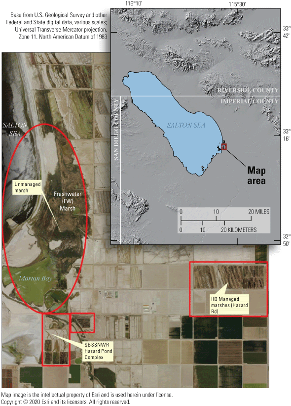
Sonny Bono Salton Sea National Wildlife Refuge (SBSSNWR) with existing marshes comprising unit 2 of the SBSSNWR and the 6-acre proposed restoration project to be created with Alamo River water are at the southwest, marshes managed by the Imperial Irrigation District (IID) are to the east, and a large unmanaged habitat maintained with agricultural drainage is located to the north of unit 2. Imperial Wildlife Area Wister Unit, north of Freshwater Marsh, not shown.
Preliminary results from surveys completed in 2014 confirmed rail use of these new and unmanaged emergent marshes (U.S. Fish and Wildlife Service, 2014b). Accordingly, their unintended creation could represent a tradeoff between increasing extant suitable habitat for an endangered species and the creation of ecological traps (in the sense of, Battin, 2004) owing to potentially harmful levels of dietary selenium exposure. Indeed, unmanaged marshes could compensate from possible decreases in managed wetlands as unimpaired Colorado River water becomes increasingly scarce and expensive (California Resources Agency, 2007). Conversely, these unmanaged marshes could act as an ecological trap for rails if elevated dietary exposure to selenium results in reduced survival and reproductive success. Moreover, selenium exposure risk to rails in these unmanaged marshes is of management concern because low salinity and high oxygen conditions typical of these marshes could increase bioavailability of selenium previously sequestered in sediments under saline conditions of the Salton Sea (Byron and Ohlendorf, 2007). Furthermore, breeding territories of most subspecies of Rallus obsoletus are restricted to small patches of emergent vegetation and corresponding food webs that reflect the local biogeochemical conditions. Consequently, the local biogeochemistry influences selenium bioavailability in rail territories (Rusk, 1991; Ackerman and others, 2012; Casazza and others, 2014).
The greater Salton Sea ecosystem continues to change owing in part to the QSA and other water-use regulations (California Resources Agency, 2007). The use of known impaired water sources by federal land managers (including within the Salton Sea) presents challenges for wetland management owing to risks to the wildlife populations that managers intend to support (Miles and others, 2009). Therefore, managers maintaining and restoring emergent marsh-dependent wildlife populations could benefit from science-based information to formulate effective water management strategies.
First, an assessment of relative selenium concentrations in water and biota sampled across spatially replicated managed and unmanaged emergent marshes during the rail breeding season would provide an indication of risk to rails and other marsh birds foraging at upper trophic levels (U.S. Department of the Interior, 2007; McKernan and others, 2016;Salton Sea Management Program, 2017). Spatial and temporal variation in selenium risk is expected given the variable selenium loadings of tile versus tail water in agricultural drains emptying into unmanaged marshes and seasonally dynamic biogeochemical conditions that affect selenium bioavailability in wetland food webs (Miles and others, 2009; Saiki and others, 2012). Furthermore, concentrations of trace elements, like selenium, in prey provide a useful proxy for exposure risk to the local rail populations (Casazza and others, 2014).
Second, an assessment of selenium risk associated with management strategies that blend agricultural drainage water with direct delivery of Colorado River water for the creation of new emergent-marsh habitats could be particularly useful to federal land managers. For example, all available habitat for rails managed by the U.S. Fish and Wildlife Service (USFWS) Sonny Bono Salton Sea National Wildlife Refuge is sustained by direct deliveries of Colorado River water. Many of these wetlands are managed primarily for resident and migratory waterfowl habitat and sport-hunting opportunities and they experience concomitant fluctuations in seasonal water-levels and emergent vegetation cover. Existing deliveries of Colorado River water could be stretched by mixing with unrestricted flows of agricultural drainage water to dilute selenium concentrations in water inflows. However, baseline estimates of selenium exposure in managed marshes before mixing are needed because benthic food webs in some managed emergent marshes around the Salton Sea can exceed selenium toxicity thresholds (Miles and others, 2009; De La Cruz and others, 2022).
Third, statistically robust estimates of rail occupancy that account for variable probabilities of detection across available managed and unmanaged emergent marshes are needed to assess the current distribution of rails relative to potential selenium risk. This effort includes identifying marsh characteristics associated with rail occupancy. Also, estimates of rail movement rates within and among managed and unmanaged marshes using high frequency location data are necessary to determine rail site fidelity and duration of selenium dietary exposure.
Objectives
To provide timely science for managers, herein we report summary statistics for managed and unmanaged emergent marshes sampled at the Salton Sea during the rail breeding season of 2016 pertaining to (1) selenium concentrations in food webs representing dietary pathways of selenium exposure and (2) patterns of rail occupancy and inter-marsh movements, estimated abundance, and regional population size of rail. Data collection and analysis for this study was designed to provide information in support of management of Yuma Ridgway’s rail and their habitats at the Salton Sea.
Selenium
-
Quantify selenium concentrations in representative rail prey (mosquitofish and crayfish), along with concentrations in source water and invertebrates representing benthic (Chironomidae) and epipelagic (Corixidae) routes of dietary exposure in managed and unmanaged freshwater wetlands adjacent to or near the Salton Sea.
-
Further quantify these patterns temporally by sampling during periods corresponding to reproductive life-history stages of rails: (1) pre-nesting/pair formation, (2) nesting, and (3) fledgling.
-
Assess aquatic food webs of unmanaged emergent marshes and managed wetlands for differences in selenium transfer patterns and the potential contaminant exposure to rails with a focus on selenium concentrations representative of different pathways (waterboatman: epipelagic, midge larvae: benthic) and prey items (crayfish, freshwater fish).
-
Obtain baseline selenium conditions for a newly restored and federally managed emergent marsh (HZ9A) before proposed mixing of Colorado River and agricultural drainage water.
-
Determine how potential selenium exposure has changed in unmanaged marshes pre- and post-transition from saline to emergent marsh wetland (Morton Bay) and with increasing emergent vegetation cover (Freshwater [FW] Marsh).
-
Quantify selenium concentrations in blood and feather samples from adult rails captured and radio-marked at managed and unmanaged wetlands as part of a companion study of rail occupancy and movements.
Rail Population and Movements
-
Quantify rail movement and space use patterns to assess spatiotemporal extent of selenium exposure risk.
-
Estimate patterns of rail detection and abundance relative to habitat conditions from call count surveys.
-
Extrapolate abundance measures to regional population estimates for rail under specific simplifying assumptions.
Methods
We sampled and analyzed selenium concentrations in the environment (water), diet (invertebrates and fish), and body (feathers and blood) of Yuma Ridgway’s rails inhabiting marshes in the Salton Sea in 2016. In the same year, we performed rail call count surveys and telemetry designed to evaluate rail habitat use, movement, and abundance. Water, dietary, and rail samples for selenium analyses were collected from managed and unmanaged marshes in February (only water and diet), April, and June. Call count surveys were done in March and April and telemetry was completed between April and November. Selenium concentration data and survey and movement data for rails in marshlands of the Salton Sea used to support our analyses are provided in USGS data releases (Overton and others, 2022; Ricca and others, 2022, respectively).
Selenium Sampling Design
In the spring and summer 2016, we established and repeatedly sampled a total of 30 fixed points to estimate spatial and temporal variation of selenium exposure to rails within 2 unmanaged and 2 managed marshes situated near the southeastern shoreline of the Salton Sea (fig. 2). These marshes corresponded with areas acoustically sampled for rail occupancy (see the “Rail Sampling Design” section). The two unmanaged marshes were spatially connected, but Morton Bay (MB) to the south was characterized by a ring of emergent vegetation (primarily cattail Typha spp.) approximately 25–100 meters (m) wide that encompassed larger patches of open water, whereas the FW Marsh to the north was characterized by extremely dense emergent vegetation (primarily cattail and salt cedar [Tamarix spp.]) surrounding smaller pockets of open water and drainage canals. We established 15 fixed sampling points throughout the unmanaged marshes (nmb=9, nfw=6) at accessible sites (spaced systematically) to reflect a range of increasing distances from the outlets of drainage canals that sustained these marshes (fig. 2). Accessibility through dense vegetation and deep mud prohibited a truly random sampling design. Five of these points (FW-2, FW-3, MB-1, MB-2, MB-3) were sampled during previous studies (Miles and others, 2009; De La Cruz and others, 2022), which allowed for a general comparison of selenium concentration in water and invertebrate samples as habitats at these sites changed over time (from 2006–10 to 2016) from hyper- to meso- to oligo-haline wetlands (Morton Bay points) and from less dense to denser cattail and salt-cedar (FW points). The two managed marshes were characterized by a system of interconnected shallow water ponds with variable cover of emergent vegetation. The Hazard Marsh complex (HZ) was managed by the USFWS Sonny Bono Salton Sea National Wildlife Refuge (SSNWR) primarily for migratory shorebirds and waterfowl and generally experienced seasonal variation in water deliveries and vegetation management. The Imperial Irrigation District (IID) Marsh complex was managed by the IID primarily as mitigation habitat and was created in the late 2000s. We established 15 fixed sampling points throughout the managed marsh complexes (nhz=12, niid=3), with points placed near the inflow, middle, and outflow of each marsh. Four marshes were sampled at Hazard Marsh complex (HZ6, HZ3A, HZ9A, HZ10) and one marsh was sampled at IID Marsh (fig. 2). These marshes were selected to represent a wide range of emergent vegetation cover and because these marshes would remain at least partially flooded across all sampling periods. In addition, Hazard Marsh HZ9A was newly restored with cattails in 2015 by the SSNWR. Marsh HZ9A was sampled to provide baseline information on selenium risk before implementation of proposed water management, described in the “Introduction” section, that would blend unmanaged Alamo River water with direct deliveries of Colorado River to reduce selenium risk.
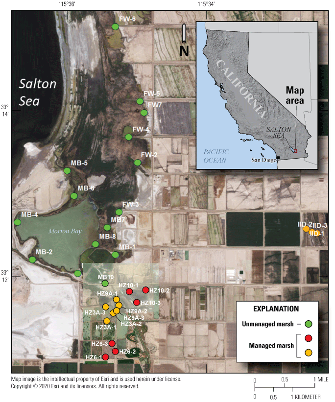
Fixed sampling points (30) established for environmental and dietary selenium risk to Yuma Ridgway’s rails occupying managed (orange points for HZ9A and IID Marshes; red points for HZ10 and HZ6 Marshes) and unmanaged (green points) marshes near the southeastern shore of the Salton Sea, California, during February, April, and June 2016.
We performed sampling to determine selenium concentrations in multiple matrices, defined as types of environmental samples (water, fish, and invertebrates), during three sampling periods that represented significant times of potential selenium exposure during key reproductive life stages for rails (table 1). Sampling during late February represented selenium exposure during the pre-nesting period and nesting pair formation; mid-April represented exposure during nesting; and mid-June represented exposure during fledging. Samples from at least one matrix were collected at all fixed points across all sampling periods except for points at the IID Marsh, which were not accessible during the February sampling period and were only sampled during the mid-April and mid-June periods.
Table 1.
Number of water, invertebrate, and fish samples collected for selenium analysis at fixed points in managed and unmanaged Salton Sea emergent marsh wetlands during February, April, and June 2016.[Site and period combinations with no samples collected are denoted by ‘–‘. Abbreviations: FW, Freshwater; IID, Imperial Irrigation District]
At each fixed point and across all sampling periods, we attempted to collect samples of (1) unfiltered surface water (for total recoverable selenium), (2) three taxonomic orders of invertebrates, and (3) two taxonomic classes of vertebrates (table 1). This sampling design reflected baseline waterborne selenium concentrations and subsequent exposure and bioaccumulation across multiple trophic levels in Salton Sea emergent marsh food webs during the rail reproductive season. Low available biomass (<0.5 grams [g], wet weight) resulted in missing analyzable samples for some matrix-point-period combinations (table 1). Whole-body samples of animal tissue were comprised of (1) Chironomidae (midge larvae), (2) Corixidae (water boatmen), (3) Gambusia spp (mosquitofish), and (4) crayfish. Corixidae are epipelagic macro invertebrates that can represent more water-borne pathways of selenium exposure to higher trophic levels, whereas Chironomidae larvae are more representative of benthic pathways (Miles and others, 2009). Mosquitofish can broadly index selenium toxicity in aquatic food webs, according to the U.S. Environmental Protection Agency (2016) guidelines, but we sampled mosquitofish and crayfish because of their ubiquity as readily apparent rail prey items (Pyle, 2008; García-Fernández and others, 2013; Overton and others, 2014; Eddleman and Conway, 202017). Lastly, head and body contour feathers, along with a smaller number of whole blood samples, were collected from rails that were captured and marked as part of the rail movement component of our study.
All biological samples were collected under California Department of Fish and Wildlife scientific collecting permits (SCP-8090) and USFWS Memoranda of Understanding (TE020548-14). Specific details regarding sampling of each matrix and subsequent analytical chemistry are listed in the next section.
Unfiltered Surface Water
We collected water samples at all fixed sampling points and across all sampling periods (except at IID Marsh; table 1). Undisturbed samples of surficial water (with algae and biofilm displaced with a simple mesh strainer) were collected and placed in 500-milliliter (mL) Trace Clean® high-density polyethylene (HDPE) bottles. Samples were placed immediately on ice, acidified (pH=2) with Optima™ nitric acid within 8 hours of collection and refrigerated before analytical chemistry. All water samples were unfiltered and represented concentrations of total recoverable selenium. Although selenium in water alone does not strongly predict bioaccumulation of selenium in upper trophic levels (Hamilton, 2004), estimates of total recoverable selenium in water represented a minimal selenium exposure baseline of biota inhabiting each marsh across all periods sampled.
Chironomidae (Midge larvae) and Corixidae (Waterboatman)
We collected composite samples of Corixidae and Chironomidae at all fixed sampling points where present in sufficient biomass and across all sampling periods (except the IID Marsh; table 1). Corixidae and Chironomidae matrices were sampled extensively in previous studies of selenium risk in Salton Sea wetland food webs (Miles and others, 2009; Saiki and others, 2010; De La Cruz and others, 202216) and are therefore useful for inter- and intra-habitat comparisons. Samples from each taxa and site were collected using a combination of techniques that included a D-ring net swept rapidly in a circular motion though the water column and from surficial sediments <5-centimeter (cm) passed through a 1.0-millimeter (mm) sieve. Invertebrates were placed in clean glass jars filled with water from the respective site for 12–24 hours to allow their guts to purge. Each sample was then sorted and rinsed in deionized water, blotted, and placed in 60-mL HDPE jars until a composite-blotted wet-weight of approximately 0.8 g was achieved. Samples were then frozen at –20 degrees Celsius (°C) before analytical chemistry.
Mosquitofish
We collected composite samples of mosquitofish at all fixed sampling sites where present in sufficient biomass and across all sampling periods (except IID Marsh; table 1). Selenium concentrations in mosquitofish likely represented a pathway of direct selenium exposure to rails given the prevalence of fish in rail diets (McKernan and others, 2016; Eddleman and Conway, 202017). Samples were collected at each point by rapidly sweeping a D-ring net through the water column or visually stalking and netting fish. An average of 12.8 (standard deviation [SD]=5.6) individual fish were collected at each site and sampling period and placed in 500-mL glass jars filled with site water. We then rinsed each fish with deionized water and blotted dry before obtaining individual whole-body mass (to the nearest 0.1 g) and standard length (nose to peduncle, to the nearest 0.1 mm). Individuals were then pooled into a composite sample for each point and sampling period. Mass and standard lengths of fish comprising composite samples averaged 0.19 g (SD=0.26) and 19.1 mm (SD=5.5), respectively. Although variation in selenium concentration and overall body burden related to variation in body size is best controlled through analyses of individual fish (Ackerman and Eagles-Smith, 2010), limited funding for analytical chemistry precluded selenium analysis of individual fish.
Crayfish
We collected crayfish representing three different size classes at fixed sampling sites where present in sufficient biomass and across all sampling periods (except for the IID Marsh; table 1). Unlike other sample matrices, we did not collect crayfish samples for all points and time periods because our objective was to focus on variation among individuals of different weight classes, and crayfish availability and capture success was highly variable. At each point, we set one to three minnow traps baited with chicken legs accessible for consumption. Traps were left out overnight and checked daily. Crayfish were processed and analyzed for selenium primarily on an individual basis within weight classes to evaluate selenium risk to rails that forage on different sizes of crayfish, as opposed to compositing different size classes that could confound measured differences in selenium concentrations among sites (Ackerman and Eagles-Smith, 2010). We rinsed each crayfish with deionized water and blotted dry. Each crayfish was then weighed to the nearest 0.01 g and length measured from rostrum to peduncle to the nearest 0.1 cm. The size classes (based on cut-points in slopes from weight to length relationships) were as follows: small=0.1–5 g, medium=5–15 g, and large>15 g. Crayfish comprising the small size class at a sampling point were composited if their individual mass was too light to allow for selenium analysis. Crayfish were analyzed for selenium on a whole-body basis.
Rail Feather and Blood
We collected samples of rail feathers and whole blood opportunistically from adult individuals captured as part of the rail telemetry part of this study and feathers from adult and juvenile individuals as part of a related rail movement study (Harrity and Conway, 2020). Samples were heavily skewed toward managed marshes because only three birds were captured from unmanaged marshes (all at Morton Bay). Managed marshes included the Hazard and IID Marshes and the Imperial Wildlife Area Wister Unit managed by the California Department of Fish and Wildlife. The Wister Unit borders the northern extent of the FW Marsh. Samples from Hazard and IID were collected from mid-March 2016 through the end of April 2016, whereas samples from Wister were collected during June 2016. Approximately five head feathers, three to five breast feathers, or both head and breast feathers were collected per individual. Feathers were cleaned of any skin or debris and then stored dry in a coin envelope. Collection of blood was dependent on bird condition during handling; blood was only taken if the bird stayed alert during processing. In those cases, blood was subsequently drawn from the femoral artery with heparinized needles and hematocrit tubes and then immediately frozen in chemically cleaned plastic vials.
Selenium Analytical Chemistry and Reporting
All selenium samples were analyzed by the Trace Element Research Lab (TERL; Texas A&M University, College Station) under established contract with the USFWS Analytical Control Facility (ACF). Selenium concentrations were determined using inductively coupled plasma mass spectroscopy (ICP-MS). Water samples were digested for 2 hours at 85 °C in HDPE containers with ultrapure nitric and hydrochloric acids. Tissue samples were digested with nitric acid and then freeze-dried and homogenized. Measures for quality assurance/quality control (QA/QC) were conducted by the TERL for two sets of analytical runs under ACF catalogs G040061 and G040062. Results for QA/QC were verified to be in accordance with standards set by the ACF. In brief, percent recovery of selenium in standard references materials averaged 100.0 (SD=5.5) in water (National Institute of Standards and Technology [NIST] 1643e) and 101.3 (SD=5.9) in tissues (NIST 2976). Percent recovery of selenium in spiked sample matrices averaged 97.7 (SD=3.3) in water and 99.1 (SD=7.2) in tissues. Relative percent difference in duplicate samples averaged 5.3 (SD=8.4) in water and 4.6 (SD=5.6) in tissues. We report all selenium concentrations in all water samples on a wet weight (ww) basis as parts per billion (or μg/L), and all tissue samples (other than blood) on a dw basis as part per million (or μg/g). Selenium concentrations in whole blood are reported as μg/g, ww. Except for one water sample, selenium was detected in all samples above the average method limit of detection (water=0.2 μg/L; tissue=0.8 μg/g, dry weight [dw]; whole blood=0.004 μg/g ww). We report estimated body burden of selenium in crayfish as the product of whole-body dry weight mass and dry weight selenium concentration (Ackerman and Eagles-Smith, 2010). For any composited small crayfish samples (n=3), we used the average whole-body dry weight mass. We report basic summary statistics (mean±2 standard error [SE]) across all marshes, sample periods, and sample matrices. We illustrate sampling distributions of selenium across marshes and sample periods for each matrix with boxplots, where boxes represent the 25th and 75th percentiles for concentrations, lines inside boxes are median values, whiskers represent the 5th and 95th percentiles, and dots represent outlying values. We then overlaid suggested toxicity thresholds or chronic values (for example, EC10) for selenium concentrations from the literature (2.0 μg/L for unfiltered water; 3.0–4.0 μg/g for invertebrates and fish [U.S. Department of the Interior, 1998; Hamilton, 2004] and calculated the percentage of samples within each marsh that exceed thresholds for each matrix. We use these thresholds for ready comparison to past studies in the study area (Miles and others, 2009) by interested readers, but we note that more recent chronic values for water and whole fish have been set forth by the U.S. Environmental Protection Agency (EPA; U.S. Environmental Protection Agency, 2016). Accordingly, where relevant, we report percentages of samples exceeding EPA chronic values for the protection of aquatic life (U.S. Environmental Protection Agency, 2016). Thresholds for rails have not been established, so we compared selenium concentrations in blood and feather samples to those reported for rails by McKernan and others (2016) and waterbirds by Ohlendorf (2003). Selenium in rail feathers reflect dietary exposure and internal depuration before molt and new feather growth (Pyle, 2008; García-Fernández and others, 2013), which corresponds to the start of the breeding season in April (Eddleman and Conway, 2020). In contrast, selenium in whole blood is a more instantaneous measure of exposure and circulating levels (García-Fernández and others, 2013; Burger and others, 2015). Finally, we present spatially explicit ‘heat maps’ depicting binned selenium concentrations at each sample location across the three sample periods for each matrix.
We used boxplots to illustrate changes in selenium concentrations in water, Chironomidae, and Corixidae sampled at the five points in the unmanaged marsh across the current and previous studies (Miles and others, 2009; De La Cruz and others, 2022). This use of boxplots allows for a visualization of trends across the generalized state-transition of these habitats over 10 years (2006–16). Time periods were pooled into three groups describing Salton Sea water elevation: (1) high (2006–07), (2) declining (2008–10), and (3) low (2016), which inversely relate to periods of high salinity and low wetland vegetation cover. We note that selenium analytical methods used in this study differ from those (EPA method 7742) used by Miles and others (2009) when Morton Bay was in a high salinity state. These analytical differences likely do not confound interpretation of trends due to the relatively high selenium concentrations reported across all studies (R. Taylor, Trace Element Research Lab, written commun., February 2, 2016).
Rail Sampling Design
Secretive Marsh-Bird Surveys
Call counts were done for rails by using protocols based on the North American Marsh Bird Monitoring Protocol (NAMBMP; Conway, 2011) along 14 current or historically occupied marshes along the southeastern edge of the Salton Sea and southern Imperial Valley. This survey method uses a series of listening stations (hereafter, transect or marsh) located at least 200 m apart and along the perimeter of accessible rail habitats. Survey period for all stations extended through the crepuscular periods and included no more than a half hour of twilight periods (before sunrise or after sunset) or an hour and a half of daylit periods (after sunrise or before sunset). Each transect was surveyed three times between March 8 and April 17, 2016, with alternating a.m. and p.m. survey periods. Two transects were surveyed a fourth time, which also was included in the analysis. Each station was surveyed for 10 minutes and included 5 minutes of passive call detection followed immediately by playback of a sequence of recorded secretive marsh bird calls. Each 1-minute-long sequence consisted of three calls played 15 seconds (second=0, 15, and 30) apart, followed by 30 seconds of silence. The species selected for call playback can be tailored to the local bird community, but we elected to use the same sequence used for NAMBMP during operational survey development in San Francisco Bay because we were only interested in providing detection information for Yuma Ridgway’s rail. The species present in our recordings were, in order of playback, black rail, Yuma Ridgway’s rail, sora, Virginia rail, and American bittern. Upon detection of a call, observers recorded the approximate (±20 m) location on a map of recent satellite imagery and distance and direction calculated to the call, along with the time of detection. Subsequent detections of the same individual were determined by visual identification when possible or “dead-reckoning” of multiple calls from the same location. Subsequent calls were recorded within survey and when the same individual was heard or seen at subsequently visited stations in a transect, but only the initial detection was analyzed in occupancy and abundance modeling.
Rail Population Modeling
Rail call count data were aggregated to represent the total number of Yuma Ridgway’s rail detections per survey session per station and analyzed using an imperfect-detection abundance model with repeated measures (Royle, 2004). This model allowed us to estimate relationships between detection of rail vocalization and temporal and environmental variables. An important clarification relevant to territorial secretive marshbirds is that our detection probabilities are not for individuals but rather occurrence and detection of a vocalization by a rail. Survey site occupancy is static between survey rounds and not necessarily by specific individuals but by a specific number of individuals. Given the despotic nature of territorial rails before breeding, we feel this assumption is valid and that any population turn-over between survey rounds represents the exchange of individuals and not the addition or removal of individuals. Additionally, we assume that calling rates are equal across individuals after accounting for environmental or seasonal factors. The resulting detection probabilities were used to estimate approximate abundance and relationships of environmental covariates, such as habitat composition and spatial arrangement, with abundance. Four factors, including some known to influence detection probability of Ridgway’s rail in San Francisco Bay (Liu and others, 2012), were assessed: period of survey (a.m. versus p.m.), Julian date, time of survey relative to dawn and dusk, and temperature. Temporal covariates were determined based on Global Positioning System (GPS) location of survey station and local sunrise and sunset timing. Temperature was recorded hourly at the closest METeorological Aerodrome Report (METAR) station (Station: KIPL, Imperial, CA) to all survey locations. Models assessing factors that affect abundance of calling Yuma Ridgway’s rail included site-level habitat characteristics derived from aerial or satellite orthoimagery.
Two methods were used to classify habitat type into two sets of habitat metrics used in subsequent analysis of rail abundance. For the first set of metrics, proportion of “Potential” habitat was delineated from orthophotos based on current and past surveyed habitats and consisted of all contiguous non-agricultural vegetation and wet areas. For the second set, potential habitats were further analyzed by performing a maximum likelihood classification of contemporaneous USGS Landsat imagery to separate vegetated from barren and open-water landcovers, resulting in a vegetated “Classified” habitat. The proportions of potential and classified habitats were measured at three spatial scales from each station: 300, 1,000, and 5,000 m. Large contiguous habitats are suspected to have greater abundance of rails in San Francisco Bay. Although use of one candidate variable, perimeter:area ratio, would have allowed investigation of the relationship between size of habitat patches and rail abundance, we excluded this variable from our analysis because it was apparent that new levees and berms had been constructed between the time of available orthoimagery and data collection.
Habitats were classified based on management type and broad composition classes. Managed marshes involved some degree of water management and anthropogenic impoundment, usually with active vegetation management (for example, mowing/burning). Unmanaged marshes contained suitable vegetation, but any impoundments were naturally formed and included no vegetation or direct water management. Habitat type was considered “dominant” if at least 80 percent of the available habitat within 300 m of a survey station was of a single management class. This classification scheme resulted in the habitat classes: “managed marsh dominant,” “unmanaged marsh dominant,” “managed: unmanaged marsh edge,” “managed: non-habitat edge,” and “unmanaged: non-habitat edge.”
Quadratic relationships were included in candidate models that estimated the effect of classified habitat type on abundance and for temperature, date, and time of day effects on detection probability. Model uncertainty was assessed using the Akaike information criterion (AIC) with ranking of competing models within the suite of candidates identified by a delta-AIC (increase in AIC scores relative to the best performing model). Models with delta-AIC scores <2 are considered nearly equivalently effective at explaining dependent variables; models with delta-AIC scores <6 are presented. We performed a priori analysis comparing model performance of the similar two groups of habitat variables “potential” versus “classified” habitat. Models incorporating the potential habitat metrics outperformed equivalent models with classified habitat metrics (in other words, at same 300-, 1,000-, and 5,000-m scale) by 3 to 6 AIC units. Therefore, we omitted classified habitat metrics from our final suite of candidate models to reduce overall model selection uncertainty. Dependent variables from the best performing model according to AIC model selection are presented as back-transformed values of variables analyzed on the logit (detection probability) or log scale (abundance). In total, we evaluated 13 formulations of detection probability and 25 formulations of rail abundance, resulting in 325 candidate models plus a null model to evaluate relative model fit.
The development of abundance estimates tied to environmental variables that influence estimates allow for extrapolation to regional estimates encompassing areas where surveys were not performed. Relationships between predictor variables and rail abundance from the best performing imperfect detection model were used to extrapolate regional estimates of rail abundance. Confounding the relationship between calls heard and abundance is that the operational NAMBMP resulted in non-independence among survey stations. Survey stations in the NAMBMP are placed 200 m apart, but rail detection extends well beyond 200 m. This non-independence between stations means that extrapolating rail abundance using a census with the same protocol as NAMBMP (200-m spacing) would effectively overrepresent parts of the landscape where adjacent survey stations are. Therefore, we provide an estimate of the total number of birds expected to be counted from a survey effort consisting of independently placed survey stations (400 m apart) that saturate available habitats in the study area. Statistical modelling was performed using the ‘pcount’ function in R package “unmarked” (https://cran.r-project.org/web/packages/unmarked/index.html; Fiske and Chandler, 2011). Habitat classification using maximum likelihood supervised classification and extrapolation of abundance estimate were performed using ArcGIS—ArcMap software (Environmental Systems Research Institute, 2011).
Rail Ultra High Frequency Telemetry
There were 16 rails captured by hand, with a long-handled net, mist net, or with the use of modified drop-door traps (Zembal and Massey, 1983; Conway and others, 1993; Albertson, 1995; Bui and others, 2015). All birds were measured, banded, radio-marked, and released in situ with minimal handling time. Capture occurred in early morning or evening to minimize heat stress. Transmitters were Ecotone© Sterna model GPS that transmitted data through ultra high frequency (UHF) radio frequencies to small portable base stations. Transmitters could be set to record locations from 1-minute to 4-hour intervals and would suspend data collection when battery levels dropped below a threshold and would be restarted upon solar recharging by top-mounted solar cells. Transmitters were attached using backpack harnesses previously used on Ridgway’s rails (Albertson, 1995; Overton and others, 2014) and all marking occurred between April 3 and April 27. Whole blood was collected (up to 1 mL) using brachial, medial metatarsal, or jugular venipuncture on 14 individuals using 24- to 28-gauge heparinized needles. To establish a tissue comparison, we collected two to three breast and head feathers collected at the time of capture to assess selenium concentrations.
All transmitters were initially deployed with a 15-minute GPS collection interval that could be maintained under full, direct sunlight (for example, while testing transmitters) but was too taxing for continuous data collection when deployed on a rail due to shading by vegetation. Transmitters that could be reconnected with a base station were adjusted to a 4-hour cycle for the remainder of the study. However, many transmitters could not reconnect and did not sufficiently recharge to enable continued tracking following the initial period of deployment. As a result, we were not able to determine the fate of most individuals due to battery failures. Geographic (World Geodetic System 1984) location data were projected to North American Datum of 1983 Universal Transverse Mercator zone 11 before analysis to facilitate estimation of home range and movement patterns in metric units.
Location data were analyzed across each individual to determine patterns of space use as indicated by spatial distribution. Point pattern analyses were used to quantify the amount of space typically used by an individual, which has relevance to territorial patterns, potential reproductive patterns (nesting), and potentially for habitat quality. Available data were analyzed across all individuals to determine the duration at which sufficient relocations had been obtained to calculate stable estimates of home range size. Once a suitable temporal range was identified, estimates of home range size across this duration were calculated with a daily incrementing start date. The time necessary for home range size to equilibrate to within 20 percent of “final” home range size for an individual was used to gauge the minimum sample size needed to develop robust home range estimates. Smaller (approximately 1.5 ha) home ranges tended to take longer to reach stability than median (approximately 2.5 ha) or larger (>4 ha) home ranges, but 75 percent of individuals reached stable home range size estimates around 5 days. Therefore, we decided to calculate home range size in weekly increments through the available period of data. Given substantial heterogeneity of vegetation and landscape features in the study area that could influence the shape and sizes of rail home ranges, weekly home range size was calculated using a kernel utilization distribution and local convex hull methods. Both kernel and local convex hull are accepted methods for analyzing space use of wild animal populations. Although kernel methods have been suggested to perform better than local convex hull generally, for species that exhibit sharp boundaries in availability of habitat or demonstrate spatial gaps due to territorial aggression among neighbors, local convex hull may more effectively limit unused area in home ranges that otherwise result in elevated bias in home range size (Lichti and Swihart, 2011). Kernels were based on least square cross-validation to estimate a smoothing parameter/bandwidth (Worton, 1989). Local convex hulls were based on the nearest neighbor method (LoCoH-k) to develop hulls across eight neighbors (Getz and Wilmers, 2004). Utilization distributions were calculated using the 95 percent-isopleth for each method, with all analysis employing the R package “adehabitatHR” (Calenge, 2006), and movement patterns were calculated using the ‘dist’ function within the core R stats package (R Development Core Team, 2017).
Results
We report spatial and seasonal patterns of selenium concentrations across all matrices sampled at the Salton Sea. We analyzed selenium concentrations from 470 samples across 7 marshes, 7 sample matrices, and 3 periods (table 2). We also report patterns of rail occupancy, movements, and abundance.
Selenium
Unfiltered Surface Water
Selenium was detected in all but one water sample. Mean concentrations (plus or minus 2 SE) are reported in table 2, and marsh sampling distributions of selenium concentration are illustrated in figure 3. Mean concentrations ranged from a low of 0.4 μg/L in managed IID Marshes during April to 2.0 μg/L in the unmanaged FW Marsh during June. Distributions of selenium concentrations of unmanaged marshes largely overlapped each other, but unmanaged marsh concentrations were higher than those from managed marshes (fig. 3). At unmanaged marshes, concentrations of samples varied substantially within marsh location and season combinations. Median concentration differed relatively little among seasons at FW Marsh, whereas the concentration median and variability of among samples declined from February to June at Morton Bay (fig. 3). At managed marshes, distributions of selenium from Hazard Marshes were distinct and higher than those at IID that most closely resembled background concentrations, and seasonal trends were not apparent at either marsh (fig. 3). Average concentrations from HZ9A were higher across all seasons (particularly in June) in comparison to concentrations averaged across all Hazard Marshes (table 2).
Table 2.
Mean (±2 standard error [SE]) concentrations for selenium in the water (micrograms per liter [µg/L] of unfiltered water) and aquatic food web samples (micrograms per gram [µg/g] dry weight animal tissue) in sites at Salton Sea (California), summarized for the two management units (Sonny Bono Salton Sea National Wildlife Refuge Hazard Marshes and Imperial Irrigation District) and two unmanaged units (Morton Bay and Freshwater Marsh), with HZ9A summarized separately because of special management status.[No values are indicated by “—”. Abbreviations: SE, standard error; µg/L, microgram per liter; µg/g, microgram per gram; FW, freshwater; IID, Imperial Irrigation District]
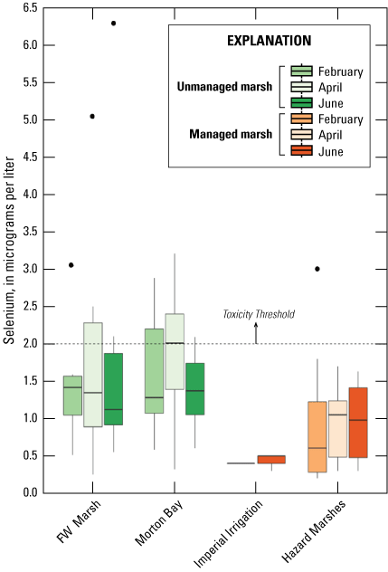
Distribution of total recoverable selenium concentrations in micrograms per liter (μg/L) in unfiltered water sampled from managed and unmanaged marshes near the southeastern shore of the Salton Sea, California, during February, April, and June 2016. Boxes represent the 25th and 75th percentiles for concentrations, line inside the box is the median, whiskers are 5th and 95th percentiles, and dots are outlying values. The dashed line represents a suggested threshold of 2.0 µg/L for aquatic food webs (U.S. Department of the Interior, 1998; Hamilton, 2004). Note that no samples were collected in Imperial Irrigation District Marshes during February.
A suggested toxicity threshold for total recoverable selenium in water is 2.0 μg/L, whereas concentrations greater than 1–2 μg/L are considered elevated above background concentrations (U.S. Department of the Interior, 1998; Hamilton, 2004). Across the study, concentrations of selenium in 29 and 33 percent of water samples from unmanaged marshes at FW Marsh and Morton Bay, in comparison to 3 percent and 0 percent of water samples from managed marshes at Hazard and IID exceeded 2.0 μg/L, respectively (fig. 4). If we assume that our measures of total recoverable selenium reflect a minimum concentration of 1.5 μg/L total dissolved selenium over a 30-day period and more than one sample collected at a fixed point over a 3-year period exceeds that concentration according to the new U.S. Environmental Protection Agency (2016) criteria for lentic systems, then chronic risk to waterborne selenium exposure is roughly 30 percent higher for aquatic life in unmanaged compared to managed marshes. Selenium concentrations consistently exceeded 2.0 μg/L across all sampling periods at FW-3 and during two (February and April) of three sampling periods at MB-1, MB-7, and MB-10 (all points near or at termini of drainage canals; see fig. 2, sampling locations; fig. 4, selenium concentrations). Finally, only two samples across the study (FW-4 during April, FW-5 during June) exceeded a previously used threshold of 5.0 μg/L for protection of aquatic life (U.S. Environmental Protection Agency, 1987).
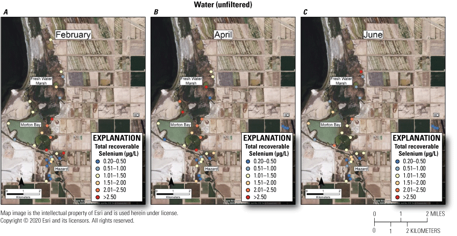
Spatially explicit concentrations of total recoverable selenium (in micrograms per liter [µg/L]) in unfiltered water collected at fixed sampling points in managed and unmanaged marshes near the southeastern shore of the Salton Sea, California, during A, February; B, April; and C, June 2016. Colors from blue to red represent relative increases in selenium and are scaled around a suggested threshold of 2.0 µg/L for aquatic food webs (U.S. Department of the Interior, 1998; Hamilton, 2004). The pink to red colors represent selenium concentrations at or above this threshold.
Chironomidae (Midge larvae) and Corixidae (Waterboatman)
Selenium was detected in all Chironomidae and Corixidae samples. Mean concentrations (plus or minus 2 SE) are reported in table 2 and sampling distributions are illustrated in figure 5. For Chironomidae, mean concentrations ranged from a low of 1.45 μg/g (dry weight) in managed IID Marshes during June to >6.0 μg/g in unmanaged FW Marsh and the managed HZ9A Marsh in Hazard during February (table 2). For Corixidae, mean concentrations ranged from a low of 1.10 μg/g in managed IID Marshes during June to 3.13 μg/g in managed Marsh HZ9A during April (table 2). Distributions across all sampling periods and marsh complexes indicated higher and largely non-overlapping concentrations of selenium in Chironomidae compared to Corixidae (fig. 5). For Chironomidae, variation in concentrations steadily tracked sampling periods, whereby concentrations at unmanaged FW Marsh and managed Hazard and IID Marshes decreased steadily across time, with relatively higher concentrations during February and April compared to much lower concentrations during June. In contrast, concentrations in Chironomidae from unmanaged Morton Bay followed an opposite seasonal pattern that increased from February to June. For Corixidae, seasonal trends were only evident at Morton Bay that followed a similar February to June increase in concentrations as seen in Chironomids from the same marsh (fig. 5). At managed marshes, distributions of selenium in both taxa from Hazard were distinct from, and higher than, those at IID. Also, distributions of selenium in both taxa from Hazard more closely resembled those at both unmanaged marshes.
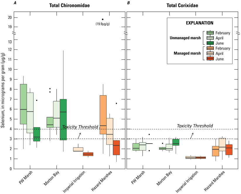
Distribution of total selenium concentrations (micrograms per gram [μg/g], dry weight [dw]) in A, Chironomidae (midge larvae); and B, Corixidae (water boatmen). Sampled from managed and unmanaged marshes near the southeastern shore of the Salton Sea, California, during February, April, and June 2016. Boxes represent the 25th and 75th percentiles for concentrations, line inside the box is the median, whiskers are 5th and 95th percentiles, and dots are outlying values. The dashed lines represent a suggested dietary threshold of 3.0–4.0 μg/g (dw) for taxa consuming invertebrates in aquatic food webs (U.S. Department of the Interior, 1998; Hamilton, 2004). Note that no samples were collected at Imperial Irrigation Marshes during February.
Suggested dietary toxicity thresholds for selenium in invertebrate avian prey range between 3.0 and 4.0 μg/g dry weight (Hamilton, 2004). For Chironomidae across the study, concentrations of selenium in 73 percent and 85 percent of samples from unmanaged marshes at FW Marsh and Morton Bay and 52 percent and 0 percent of samples from managed marshes at Hazard and IID, respectively exceeded a more protective 3.0 μg/g threshold (see fig. 2, sample locations; fig. 6, selenium concentrations). The highest concentration of selenium across all samples was detected in Chironomidae at HZ6-1 (19.9 μg/g) during February. However, abundance of Chironomidae was too low to effectively sample HZ6-1, a marsh inlet, during April and June. Chironomidae samples from FW-7 and MB-3 harbored selenium concentrations that consistently exceeded 6.0 μg/g across all three sampling periods, whereas samples from MB-7 and MB-5 exceeded 6.0 μg/g across two (April and June) of three sampling periods (see fig. 2, sample locations; fig. 6, selenium concentrations). At the managed Hazard Marsh complex, percentages of Chironomidae samples from HZ6, HZ3, and HZ9 with selenium concentrations exceeding 3.0 μg/g decreased markedly from 71 percent during February and April to 0 percent during June (fig. 6). In contrast, selenium concentrations in 33 percent and 50 percent of Chironomidae samples across the study from HZ10 exceeded 6.0 μg/g and 3.0 μg/g, respectively. For Corixidae, selenium concentrations exceeded 3.0 μg/g in 13 percent and 11 percent of samples from unmanaged FW Marsh and Morton Bay and 16 percent and 0 percent of samples from managed Hazard and IID Marshes, respectively (fig. 7). No sampled concentrations of selenium in Corixidae exceeded 4.0 μg/g. “Hot spots” with Corixidae concentrations exceeding 3.0 μg/g among unmanaged marshes included FW-7 during April and June, MB-7 during April, and MB-3 and MB-8 during June. Among managed marshes, similar hot spots occurred at all sampling points in HZ9A and HZ10-1 during April and at HZ10-2 during February. These overall patterns of higher selenium concentrations in Chironomidae compared to Corixidae, as well as relatively high percentages of Chironomidae samples from both unmanaged marshes and from Hazard that exceeded dietary thresholds are similar to patterns reported by Miles and others (2009) and De La Cruz and others (2022) in the same marsh complexes from 2006 through 2010.
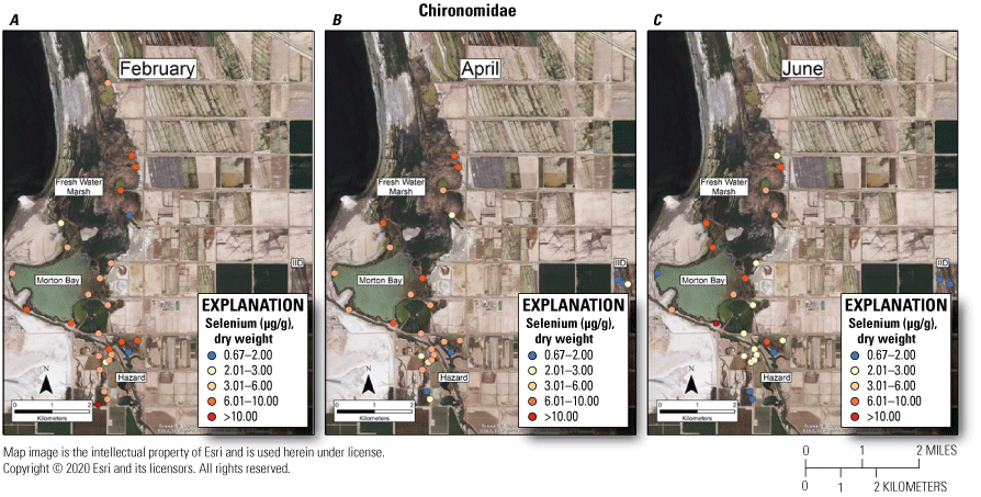
Spatially explicit concentrations of total selenium (micrograms per gram [µg/g], dry weight [dw]) in Chironomidae (midge larvae) collected at fixed sampling points in managed and unmanaged marshes near the southeastern shore of the Salton Sea, California, during A, February, B, April, and C, June 2016. Colors from blue to red represent relative increases in selenium and are scaled around a minimum suggested threshold of 3.0 µg/g (dw) for taxa consuming invertebrates in aquatic food webs (U.S. Department of the Interior, 1998; Hamilton, 2004). The pink to red colors represent selenium concentrations at or above this threshold.
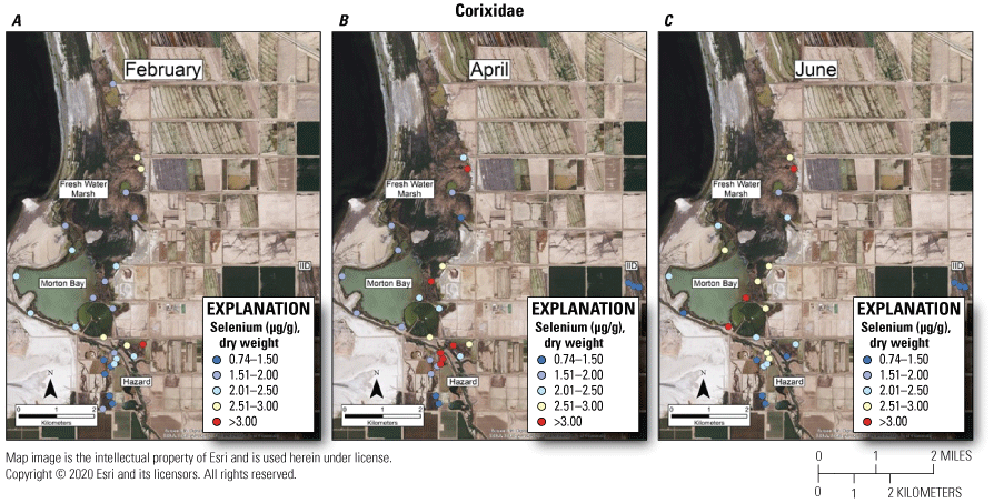
Spatially explicit concentrations of total selenium (micrograms per gram [µg/g], dry weight [dw]) in Corixidae (water boatmen) collected at fixed sampling points in managed and unmanaged marshes near the southeastern shore of the Salton Sea, California, during A, February; B, April; and C, June 2016. Colors from blue to red represent relative increases in selenium, and are scaled around a minimum suggested threshold of 3.0 µg/g (dw) for taxa consuming invertebrates in aquatic food webs (U.S. Department of the Interior, 1998; Hamilton, 2004). The red color represents selenium concentrations at or above this threshold.
Mosquitofish (Gambusia spp.)
Selenium was detected in all mosquitofish (Gambusia spp.) samples. Mean concentrations (±2 SE) are reported in table 2 and sampling distributions are illustrated in figure 8. Mean concentrations ranged from a low of 2.51 μg/g in managed IID Marshes during June to a high of 5.42 μg/g in Hazard Marsh HZ9A also during June (table 2). Distributions of selenium concentrations across all marsh complexes showed relatively low variation among sampling periods. Among marshes, distributions indicated generally higher selenium concentrations in mosquitofish from unmanaged marshes and the managed Hazard Marshes (where all median concentrations exceeded 3.0 μg/g) compared to the IID Marshes (fig. 8).
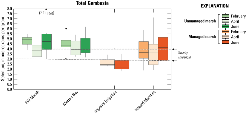
Distribution of total selenium concentrations (micrograms per gram [μg/g], dry weight [dw]) in mosquitofish (Gambusia spp.) sampled from managed and unmanaged marshes near the southeastern shore of the Salton Sea, California, during February, April, and June 2016. Boxes represent the 25th and 75th percentiles for concentrations, line inside the box is the median, whiskers are 5th and 95th percentiles, and dots are outlying values. The dashed lines represent a suggested dietary threshold of 3.0–4.0 μg/g (dw) for taxa consuming invertebrates in aquatic food webs, which was used as surrogate for fish (U.S. Department of the Interior, 1998; Hamilton, 2004). Note that no samples were collected at Imperial Irrigation (IID) Marshes during February.
To assess relative dietary risk to rails from consuming mosquitofish, we used the upper suggested dietary threshold of 4.0 μg/g (dry weight) for taxa consuming invertebrates in aquatic food webs (U.S. Department of the Interior, 1998; Hamilton, 2004) as a surrogate for consuming fish. Across the study, concentrations of selenium in 67 percent and 56 percent of samples from unmanaged marshes at FW Marsh and Morton Bay and 43 percent and 0 percent of samples from managed marshes at Hazard and IID, respectively exceeded 4.0 μg/g (fig. 9). No sampled concentrations in mosquitofish exceeded the more recent chronic value of 8.5 μg/g (dry weight) for selenium in whole fish samples (U.S. Environmental Protection Agency, 2016). However, during June, mosquitofish from FW-7 harbored 7.9 μg/g of selenium, which approached the 8.5 μg/g chronic value. Among unmanaged marshes, relative hot spots where selenium exceeded 4.0 μg/g across all sampling periods included FW-3, FW-5, FW-7, MB-3, MB-4, MB-7, and MB-8. Among managed marshes, HZ10-1, HZ10-2, and all points within HZ9A exceeded 4.0 μg/g across all sampling periods (see fig. 2, sample locations; fig. 9, selenium concentrations).
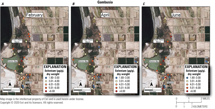
Spatially explicit concentrations of total selenium (micrograms per gram [µg/g], dry weight [dw]) in mosquitofish (Gambusia spp.) collected at fixed sampling points in managed and unmanaged marshes near the southeastern shore of the Salton Sea, California, during A, February; B, April; and C, June 2016. Colors from blue to red represent relative increases in selenium, and are scaled around an upper suggested threshold of 4.0 µg/g (dw) for taxa consuming invertebrates in aquatic food webs, which was used as surrogate for fish (U.S. Department of the Interior, 1998; Hamilton, 2004). The pink to red colors represent selenium concentrations at or above this threshold.
Crayfish
Selenium was detected in all crayfish samples. Mean concentrations (±2 SE) are reported in table 2, and sampling distributions for selenium concentrations and body burden are illustrated in figures 10 and 11, respectively. Mean concentrations of selenium in all size classes of crayfish were generally lowest (1.02–2.13 μg/g) for managed IID Marshes across sampling periods, although concentrations also were relatively low for medium-sized crayfish in Hazard Marshes across periods (1.96–2.13 μg/g). Concentrations in small and large crayfish were highest (small=4.84 and large=2.51 μg/g) during June in the unmanaged Morton Bay Marshes; concentrations in medium-sized crayfish were highest (3.47 μg/g) in FW Marsh during April. No crayfish of any size-class were captured from HZ9A during any sampling event (table 2), and sample sizes varied substantially across marshes and sampling periods (table 1).
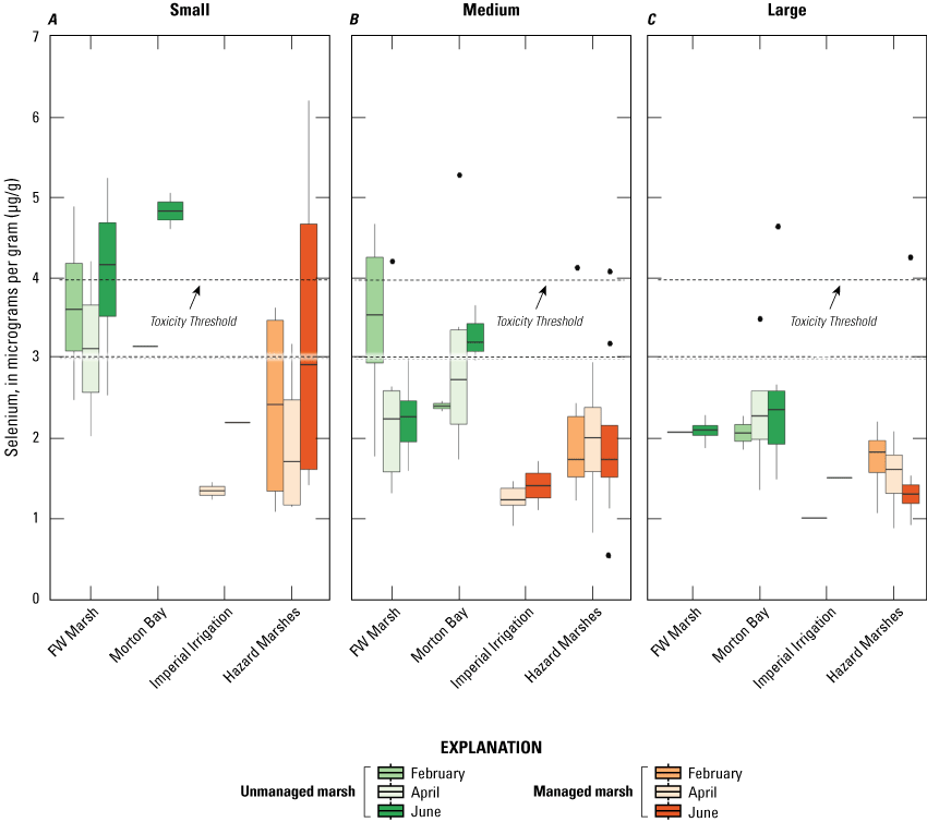
Distribution of total selenium concentrations (micrograms per gram [μg/g], dry weight [dw]) in A, small (<5 grams); B, medium (5–15 grams); and C, large (>15 grams) sized crayfish sampled from managed and unmanaged marshes near the southeastern shore of the Salton Sea, California, during February, April, and June 2016. Boxes represent the 25th and 75th percentiles for concentrations, line inside the box is the median, whiskers are 5th and 95th percentiles, and dots are outlying values. The dashed lines represent a suggested dietary threshold of 3.0–4.0 μg/g (dw) for taxa consuming invertebrates in aquatic food webs (U.S. Department of the Interior, 1998; Hamilton, 2004). Note that no samples were collected at Imperial Irrigation (IID) Marshes during February, and samples were not collected at all sample point–season combinations.
Distribution of total selenium body burden (micrograms per crayfish, dry weight [dw]) in A, small (<5 grams); B, medium (5–15 grams); and C, large (>15 grams) sized crayfish sampled from managed and unmanaged marshes near the southeastern shore of the Salton Sea, California, during February, April, and June 2016. Y-axis values vary among size-classes. Boxes represent the 25th and 75th percentiles for concentrations, line inside the box is the median, whiskers are 5th and 95th percentiles, and dots are outlying values. The dashed lines represent a suggested dietary threshold of 3.0–4.0 μg/g (dw) for taxa consuming invertebrates in aquatic food webs (U.S. Department of the Interior, 1998; Hamilton, 2004). Note that no samples were collected at Imperial Irrigation (IID) Marshes during February, and samples were not collected at all sample point–season combinations.
Distributions of selenium concentrations across all marsh complexes showed high variation among sampling periods (fig. 10). Among small crayfish, distributions from FW and Hazard Marshes indicated relatively higher selenium concentrations during February and June and lower concentrations during April. Median concentrations of both unmanaged marsh complexes exceeded 3.0 μg/g across all periods, whereas in managed marshes, concentrations did not exceed 3.0 μg/g in any period. For medium-sized crayfish, distributions from FW Marsh indicated relatively higher selenium concentrations during February and lower concentrations during April and June, whereas distributions from Morton Bay Marshes followed an opposite seasonal pattern. No strong seasonal pattern was evident for distributions at any managed marsh. Among large crayfish, steadily decreasing distributions over sampling periods from Hazard Marshes was the only seasonal pattern evident. Among marshes, distributions indicated generally higher selenium concentrations in crayfish from all size-classes and sampling periods from unmanaged compared to managed marshes. Among size-classes, concentrations were generally higher in small crayfish and lower in large crayfish (fig. 10).
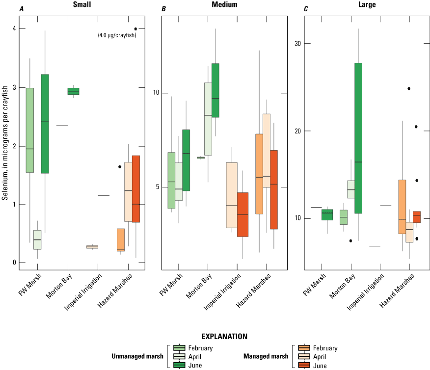
When selenium concentrations are converted to body burdens of total selenium to account for size-related variation in dietary exposure to higher trophic levels, distributions were highly variable among marshes and sampling periods (fig. 11). However, distributions of body burden selenium for large crayfish were generally at least 10 times higher compared to those from small crayfish. As within concentrations, distributions of body burden selenium were higher at unmanaged than managed marshes across most sampling periods and size class, although burdens were notably low for small size-class crayfish from FW Marsh during April. Across sampling periods and marshes, selenium body burdens followed patterns opposite of those observed for concentration, where maximum burdens for small crayfish approached 4 micrograms (μg) of selenium, medium crayfish approached 15 μg, and large crayfish approached 30 μg.
As with mosquitofish, we used the upper suggested dietary threshold of 4.0 μg /g (dw) for taxa consuming invertebrates in aquatic food webs (U.S. Department of the Interior, 1998; Hamilton, 2004) as a surrogate for consuming fish. Patterns indicated higher risk on a concentration basis for small versus large crayfish. Among small crayfish across the study, concentrations of selenium in 38 percent and 67 percent of samples from unmanaged marshes at FW Marsh and Morton Bay compared to 17 percent and 0 percent of samples from managed marshes at Hazard and IID, respectively exceeded 4.0 μg/g (fig. 12). Among medium-sized crayfish across the study, concentrations of selenium in 14 percent and 9 percent of samples from unmanaged marshes at FW Marsh and Morton Bay and 11 percent and 0 percent of samples from managed marshes at Hazard and IID, respectively exceeded 4.0 μg/g (fig. 13). Among large size-class crayfish across the study, concentrations of selenium in 0 percent and 7 percent of samples from unmanaged marshes at FW Marsh and Morton Bay compared to 4 percent and 0 percent of samples from managed marshes at Hazard and IID, respectively exceeded 4.0 μg/g (fig. 14). Sampling at fixed points was too variable to assess hot spots exceeding 4.0 μg/g across sampling periods and size-classes.

Spatially explicit concentrations of total selenium (microgram per gram [µg/g], dry weight [dw]) in small size-class (<5 g) crayfish collected at fixed sampling points in managed and unmanaged marshes near the southeastern shore of the Salton Sea, California, during A, February; B, April; and C, June 2016. Colors from blue to red represent relative increases in selenium and are scaled around an upper suggested threshold of 4.0 µg/g (dw) for taxa consuming invertebrates in aquatic food webs, which was used as surrogate for crayfish (U.S. Department of the Interior, 1998; Hamilton, 2004). The red colors represent selenium concentrations at or above this threshold and the pink color represents concentrations between 3.0 and 4.0 µg/g. For some months, the abundance of this size class was too low to sample at all points.
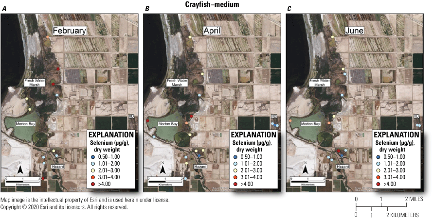
Spatially explicit concentrations of total selenium (micrograms per gram [µg/g], dry weight [dw]) in medium size-class (5–15 grams) crayfish collected at fixed sampling points in managed and unmanaged marshes near the southeastern shore of the Salton Sea, California, during A, February; B, April; and C, June 2016. Colors from blue to red represent relative increases in selenium and are scaled around an upper suggested threshold of 4.0 µg/g (dw) for taxa consuming invertebrates in aquatic food webs, which was used as surrogate for crayfish (U.S. Department of the Interior, 1998; Hamilton, 2004). The red color represents selenium concentrations at or above this threshold and the pink color represents concentrations between 3.0 and 4.0 µg/g. For some months, the abundance of this size class was too low to sample at all points.
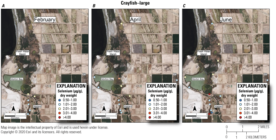
Spatially explicit concentrations of total selenium (micrograms per gram [µg/g], dry weight [dw]) in large size-class (>15 grams) crayfish collected at fixed sampling points in managed and unmanaged marshes near the southeastern shore of the Salton Sea, California, during A, February; B, April; and C, June 2016. Colors from blue to red represent relative increases in selenium and are scaled around an upper suggested threshold of 4.0 µg/g (dw) for taxa consuming invertebrates in aquatic food webs, which was used as surrogate for crayfish (U.S. Department of the Interior, 1998; Hamilton, 2004). The red colors represent selenium concentrations at or above this threshold and pink colors represent concentrations between 3.0 and 4.0 µg/g. For some months, the abundance of this size class was too low to sample at all points.
Rail Blood and Feathers
Selenium was detected in all rail tissue matrices. Mean concentrations (±2 SE) and sample sizes from opportunistic collections from rails captured as part of the movement component of the study are shown in table 3, and sampling distributions for selenium concentrations in feathers and blood are illustrated on figures 15 and 16, respectively. Additionally, spatially explicit selenium concentrations for feathers and whole blood are illustrated in figure 17. All blood samples (n=12) were collected in April. Feather samples were collected in April for rails at Hazard and IID Marshes (except for one in June); April (n =3) and June (n=2) for rails at Morton Bay; and June for rails at Wister. No rails were captured and sampled from HZ9A.
Table 3.
Descriptive statistics for selenium concentrations in head feather, body feathers, and whole blood of Yuma Ridgway’s rails from managed and unmanaged marshes near the southeastern shore of the Salton Sea, California, during April and June 2016.[Samples from Wister Unit were approximately 1 kilometer north of the Freshwater Marsh. Not all head and body feather samples were paired from the same individual. Abbreviations: Se, selenium; n, standard nomenclature to indicate sample size; µg/g, microgram per gram; dw, dry weight; ww, wet weight; SE, standard error; IID, Imperial Irrigation District]
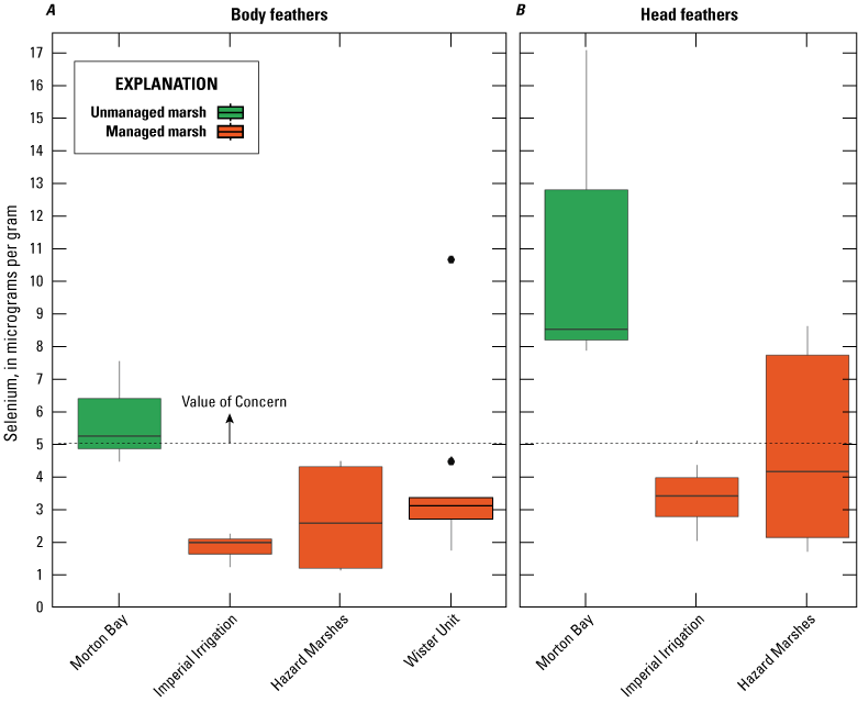
Distribution of total selenium concentrations (micrograms per liter [μg/g], dry weight [dw]) in A, body; and B, head feathers sampled from Yuma Ridgway’s rails captured in managed and unmanaged marshes near the southeastern shore of the Salton Sea, California, during April and June 2016. Boxes represent the 25th and 75th percentiles for concentrations, line inside the box is the median, whiskers are 5th and 95th percentiles, and dots are outlying values. The dashed line represents a suggested level of concern of 5.0 μg/g (dw; McKernan and others, 2016). Note: “Imperial Irrigation” represents IID indicated in main text of manuscript.
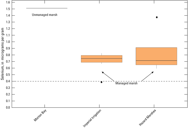
Distribution of total selenium concentrations (micrograms per gram [μg/g], wet weight) in whole blood sampled from Yuma Ridgway’s rails captured in managed and unmanaged marshes near the southeastern shore of the Salton Sea, California, during April 2016. Boxes represent the 25th and 75th percentiles for concentrations, line inside the box is the median, whiskers are 5th and 95th percentiles, and dots are outlying values. The dashed line represents background concentrations of 0.4 μg/g (wet weight) U.S. Department of the Interior (1998, p. 167). Note: “Imperial Irrigation” represents IID indicated in main text of manuscript.
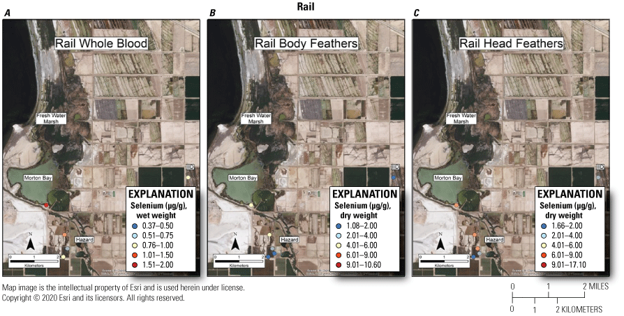
Spatially explicit concentrations of total selenium in wet weight in A, whole blood (µg/g, ww); dry weight in B, body feathers (µg/g, dw); and dry weight in C, head feathers (µg/g, dw) sampled from Yuma Ridgway’s rails captured in managed and unmanaged marshes near the southeastern shore of the Salton Sea, California, during April and June 2016 at figure 2 sampling sites. Concentrations for rails sampled at Wister are not shown.
Low sample size precluded strong inference to populations, but general trends were apparent. Distributions of selenium concentrations in head and body feathers were generally higher in rails from Morton Bay compared to those from all managed marshes (fig. 15). Head feather selenium concentrations were generally higher than concentration in body feathers among marshes (fig. 15) and head and body feather concentrations were strongly correlated with each other among paired samples (r2 0.92, n=14). Among limited blood samples, the lone sample from Morton Bay had a higher selenium concentration (1.51 μg/g, ww) than samples from managed marshes, although, one sample from Hazard Marshes had similar concentration (1.37 μg/g, ww; fig. 16).
Avian species display a wide range of sensitivity to selenium (Burger and others, 2015), and tolerance to selenium generally increases with salt-tolerance (Hamilton, 2004; Presser and Luoma, 2010). U.S. Department of the Interior (1998, p. 167) suggested feather and blood selenium concentrations below 4.0 μg/g (dw) and 0.4 μg/g (ww), respectively, reflect background concentrations, and McKernan and others (2016) suggested a concentration of 5.0 μg/g (dw) in rails that could warrant concern. Among unmanaged marshes, 100 percent of head feathers and 40 percent of body feathers sampled exceeded 5.0 μg/g (fig. 15). Among managed marshes, 50 percent and 0 percent of head and body feather samples, respectively, from Hazard Marsh, and 0 percent of all head and body feathers from IID, exceeded 5.0 μg/g. Only one (8 percent) of the body feather samples from Wister exceeded 5.0 μg/g. All blood samples, except one at IID, exceeded background concentrations of 0.4 μg/g (fig. 16).
Time Series of Selenium in Unmanaged Marshes with Lowering Salton Sea Elevation
Distributions of total recoverable selenium in unfiltered water, collected from five fixed-sampling points (FW-2, FW-3, MB-1, MB-2, MB-3), indicated an overall drop in concentrations from 2006 to 2010 when the Salton Sea was at higher elevation and the FW Marsh was less vegetated, compared to conditions in 2016 (fig. 18). In particular, during 2016, distributions from FW-2, MB-2, and MB-3 were lower and completely non-overlapping from those in 2006–10. Median selenium concentrations for 4 out of 5 points were at or below the 2.0 μg/L threshold during 2016. Selenium concentrations in Chironomidae also appeared to drop over time in some fixed sampling points (fig. 19). During 2016, distributions of selenium from FW-2 and MB-1 were lower and did not overlap those from 2008 to 2010, whereas distributions from FW-3, MB-2, and MB-3 overlapped among time periods. Greater proportions of pre-2016 selenium concentrations in Chironomidae exceeded dietary thresholds of 3.0–4.0 μg/g compared to those from 2016. We note that conditions were too saline in Morton Bay to support Chironomidae during 2006–08. Distributions of selenium in Corixidae among time periods were more variable, and non-overlapping declines during 2016 were most evident at FW-3, MB-1, and MB-2 (fig. 20). Like Chironomidae, selenium concentrations for Corixidae before 2016 (especially 2008–10) exceeded 3.0–4.0 μg/g in higher proportion than during 2016 (fig. 20). These overall patterns among water and invertebrate selenium distributions correlated with the state-transition that occurred following 2010, when Morton Bay became isolated completely from the Salton Sea and was colonized by cattails and the FW Marsh became more densely vegetated. However, this pattern may be confounded, to some extent, by differences in selenium analytical chemistry, and results should not be broadly extrapolated.
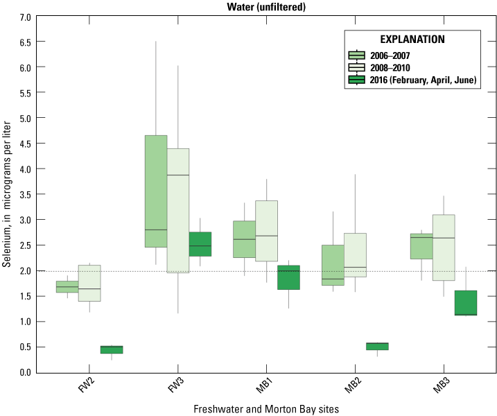
Distributions of total recoverable selenium concentrations in micrograms per liter (μg/L) along a time series of water samples from fixed points in unmanaged marshes. Periods were pooled into three groups describing Salton Sea water elevation: (1) high (2006–07), (2) declining (2008–10), and (3) low (2016), which inversely relate to periods of high salinity and low wetland vegetation cover. Boxes represent the 25th and 75th percentiles for concentrations, line inside the box is the median, whiskers are 5th and 95th percentiles, and dots are outlying values. The dashed line represents a suggested threshold of 2.0 µg/L for aquatic food webs (U.S. Department of the Interior, 1998; Hamilton, 2004).
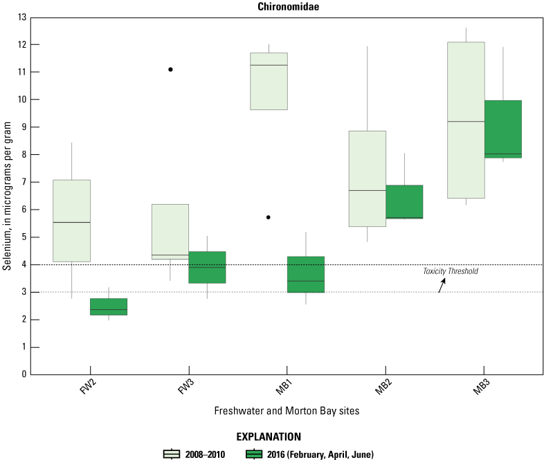
Distributions of total selenium concentrations in micrograms per gram (μg/g; dw, dry weight) along a time series of Chironomidae samples from fixed points in unmanaged marshes. Time periods were pooled into two groups describing Salton Sea water elevation: (1) declining (2008–10) and (2) low (2016), which inversely relate to periods of high salinity and low wetland vegetation cover. Boxes represent the 25th and 75th percentiles for concentrations, line inside the box is the median, whiskers are 5th and 95th percentiles, and dots are outlying values. The dashed lines represent a suggested dietary threshold of 3.0–4.0 μg/g (dw) for taxa consuming invertebrates in aquatic food webs (U.S. Department of the Interior, 1998; Hamilton, 2004). Salinity concentrations in water were too high to support Chironomidae during the high (2006–07) Salton Sea water elevation period.
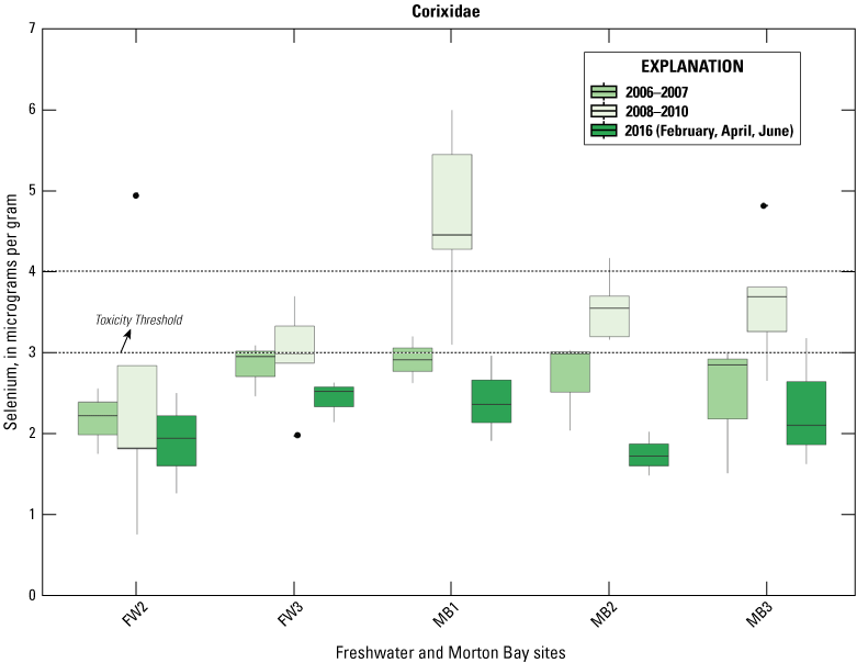
Distributions of total selenium concentrations in micrograms per gram (μg/g; dw, dry weight) along a time series of Corixidae samples from fixed points in unmanaged marshes. Time periods were pooled into three groups describing Salton Sea water elevation: (1) high (2006–07), (2) declining (2008–10), and (3) low (2016), which inversely relate to periods of high salinity and low wetland vegetation cover. Boxes represent the 25th and 75th percentiles for concentrations, line inside the box is the median, whiskers are 5th and 95th percentiles, and dots are outlying values. The dashed lines represent a suggested dietary threshold of 3.0–4.0 μg/g (dw) for taxa consuming invertebrates in aquatic food webs (U.S. Department of the Interior, 1998; Hamilton, 2004).
Rail Population and Movements
Rail Population Modeling
Among the 14 transects surveyed, call count surveys for rails resulted in 269 individual rail detections (85 stations; table 4), which included a total of 245 individual surveys across stations. Zero rails were detected at 3 (21 percent) transects, the greatest total number of detections along a transect was 48, and the greatest number of detections in a single round of surveys was 25 calls. The greatest number of calls detected at a station was six calls (in a single survey).
Table 4.
Yuma Ridgway’s rail detections in marshes of the Salton Sea, from 85 survey stations, along 14 call count transects surveyed 3 times during March 8–April 17, 2016, using the North American Marsh Bird Monitoring Protocol (Conway, 2011).On average, across all observations, estimated call detection probability at a survey station was 19.6 percent and mean number of rail calls detectable around each station was 5.1 calls among stations where detection was confirmed (approximately 1 call per station among all stations). Our candidate suite of models was effective at identifying factors associated with variation in rail call detection probability and estimated rail abundance. Our top model performed 43.8 delta-AIC units better than the null model; that did not account for variation in detection probability or rail abundance (table 5). The formulation of the detection probability was the primary source of model uncertainty of the imperfect detection modelling. Among the 326 models, the top 7 differed only in the factors identified as being most closely associated with difference in detection probability (table 5). For each of these models, which included all models up to a delta-AIC of 4, abundance of rails was estimated to vary non-linearly with the quantity of habitat adjacent to the survey station (within 300 m; fig. 21) and increased as the total habitat within 5 kilometers (km) of the survey station increased (fig. 22). These models suggest that Yuma Ridgway’s rail abundance, like Ridgway’s rail abundance in San Francisco Bay (Liu and others, 2012), is influenced by landscape level habitat availability and that smaller and isolated habitats have fewer rails. Detection probability was nearly identically described (delta-AIC <2) in four models that included temperature at the time of the survey (table 5). Thus, model selection indicated that although temperature and time of day are strongly correlated variables, call occurrence was more precisely estimated using temperature at the time of the survey than the time of the survey more generally. The top model included only a temperature effect on detection probability and estimated just over a 1.8 percent decrease in detection probability for every degree increase in temperature during the survey. The three other competing models each included temperature along with additional influence of either specific habitat type at the survey station (delta-AIC=1.15), curvilinear (delta-AIC=1.4), or linear (delta-AIC=1.999) relationship with date of the survey. The relationship between detection probability and habitat was not very strong. Detection probabilities were highest at stations near the edges of managed or unmanaged marshes (about 50 percent of the land around a station was either habitat type), whereas detection probability was significantly lower where managed and unmanaged marshland met (100 percent habitat cover). Detection probabilities within marsh fragments (<25-percent habitat around a point) or at contiguous habitats, either managed or unmanaged, were not significantly different than any other habitat class.
Table 5.
Best performing imperfect detection models (and null model) quantifying Yuma Ridgway’s rail detection probability and habitats associated with abundance in marshes of the Salton Sea (California) during spring of 2016.[Only models with delta-Akaike information criterion (AIC) values within 6 units of the best performing model are presented. All four competing models (delta-AIC less than 2.0) differed only in descriptors of detection probability. These and the next three best ranked models included the same factors associated with rail abundance. Abbreviations: w/i, within; m, meters; km, kilometers; +, plus; AM/PM, before midday/after midday]
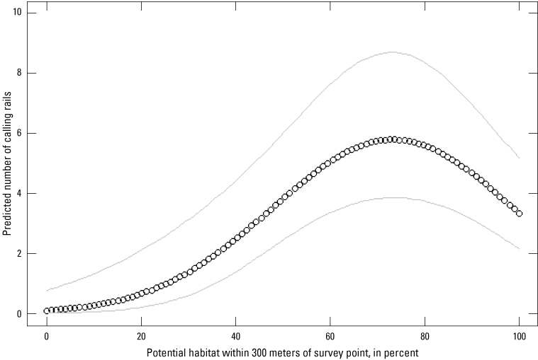
In all top performing models (delta-AIC<2.0) considered, the abundance of Yuma Ridgway’s rail in marshes of the Salton Sea (California) during spring of 2016 was predicted to vary non-linearly with quantity of habitat within 300 meters of a survey point and demonstrated greatest abundance along habitat edges. Model predictions shown are based on the best performing model.
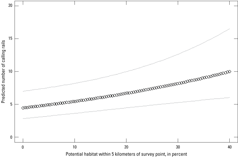
In all top performing models (delta-AIC<2.0) considered, the abundance of Yuma Ridgway’s rail in marshes of the Salton Sea (California) during spring of 2016 was predicted to increase with the total quantity of habitat within 5 kilometers of a survey point. This reflected higher population abundance near the core, or among larger, and more interconnected habitat patches with lower abundance among fragmented and isolated habitats. Model predictions shown are based on the best performing model.
Classification of remotely sensed imagery using unsupervised maximum likelihood classification techniques did not result in a stronger relationship between estimated rail abundance and habitat metrics. The top 21 models (delta-AIC <10.2) included only potential habitat as identified from past orthophoto interpretation, which could include large areas of open water and barren ground that do not provide high quality rail habitat on their own. Lack of support for the predicted relationship between call abundance and classified habitat, based on more refined maps, could be due to the relatively narrow range of classified habitats at our observation points but is likely influenced by the observed greater abundance (and potentially detection probability) along habitat edges. As a result, models including potential habitat estimated lower abundance per hectare of habitat than models including classified habitat but had a more consistent relationship across all observed data. In addition, the top performing classified habitat maps tended not to include the amount of classified habitat at the 300-m scale, and this could result from imprecision in estimates due to the relatively large, 30-m pixel size present in Landsat data.
We produced population size estimates by extrapolating the habitat relationships of the best performing imperfect detection model to characteristics of the landscape with survey stations situated to perform a complete census of available habitat (fig. 23). Major limitations of this approach include the inability to assign fine-scale habitat relationships such as vegetation composition or plant cover to imperfect detection models. In addition, the model is only able to provide estimates of the number of uniquely calling individuals detected and it remains ambiguous how this value relates to the total number of individuals within the population. Despite its limitations, our approach allowed a complete survey without double-counting rails. Such a complete survey of the southern Salton Sea and Imperial Valley result in an expected detection (that is, accounting for imperfect detection) of 1,752 rails. This estimate for rail population size in 2016 could be low compared to most years because other research indicates counts of Yuma Ridgway’s rail populations at the Salton Sea likely were lowest in 2016 for the 13-year period of 2006–18 (fig. s11 in Harrity and others, 2020).
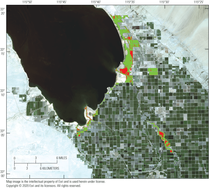
Available Yuma Ridgway’s rail vegetated habitats (green) and unvegetated marsh components (bare ground, open water; red) in marshes of the Salton Sea (California), during spring of 2016, used to extrapolate population abundance from the best performing imperfect detection model.
Although we did not evaluate relationships of finer-scale vegetation cover characteristics as indicated earlier, landscape characteristics used to define potential habitat (fig. 23) and supported by model selection (table 5) are heuristically related to other remotely sensed vegetation characteristics important in other models predicting relative rail abundance (Harrity and others, 2020). Similarities and differences between the two models could help determine how the models may be complementary for identifying suitable rail habitat in the future. Also, estimation of rail population sizes based on respective models would allow comparison and replication of their predictions based on differing assumptions and methods. In turn, managers might better be able to assess risk to the Yuma Ridgway’s rail in the Salton Sea by using a range of predicted population estimates.
We are careful to ascribe the earlier estimate (1,752 rails) to the “number of detected rails” because survey methodology relies on a bird to vocalize in order to be “present” for the survey. The call frequency of Yuma Ridgway’s rail is unknown and likely varies according to breeding stage, age, and sex. If rails call frequently and most of the population is “available” to be heard within a survey period, then our extrapolation is likely close to a true population estimate. However, if rails call infrequently and only a small fraction of the population is detected during a survey, then our abundance estimates for “calling” rails could be much lower than actual population size. At the time of this study, there is no clear mechanism available to relate detected calls, even with extrapolation to account for detection probability, to the number of individuals in the population. Estimates of calling rate or means to assign individual identity to calls heard are two approaches that could provide insight to this relationship. For example, if the average time between calls for an individual rail is substantially less than the duration of a survey at a station then our estimated number of detected calls should be much closer to the true population size than if a rail only calls once per hour. Surveying captive birds with known population size or marking individuals with sound sensing transmitters are two approaches that can be leveraged to estimate a relationship between calls heard and actual population size.
Rail Intra- and Inter-Marsh Movements
Over 5,000 locations were obtained from 15 radio-marked Yuma Ridgway’s rail covering a period from early April through mid-November 2016 (table 6). A sixteenth individual was radio-marked but the transmitter failed and never provided any locations. Due to an error in programing the transmitter duty cycle, each transmitter was initially deployed to collect locations once every 15 minutes. This schedule was too taxing on the lithium polymer batteries and transmitters were remotely reprogrammed to collect data every 4 hours; however, several transmitters suffered premature battery failure due to this early setting (table 6). Only four birds disappeared while transmitters still retained enough charge for data transmission, indicating that they moved from the marshes and could not be relocated due to the limited transmission range of the UHF transmitters (a few hundred m; table 7). The transmitter for a fifth individual was recovered with a broken harness consistent with a depredation, but no carcass or feathers were found at the site, suggesting it could have broken due to wear or damage.
Table 6.
Number of Global Positioning System relocations, primary relocation interval, and total duration of track for 15 Yuma Ridgway’s rail radio-marked in marshes of the Salton Sea (California) during early April to early November 2016.[%, percent]
Table 7.
Transmitter battery voltage and status at last location of Global Positioning System transmitters used to track Yuma Ridgway’s rail in marshes of the Salton Sea (California) during early April to early November 2016.Weekly home range size, estimated using kernel utilization distributions, ranged from 0.27 to 29.67 hectares (ha), and the average weekly kernel utilization distribution was 3.33 ha (median: 2.5 ha; fig. 24). Home range size for Yuma rails was larger than the estimated size of home ranges for Ridgway’s rail in San Francisco Bay (Rohmer, 2010; U.S. Geological Survey, unpub. data, 2015). Due to abrupt edges in habitat patches in this landscape as well as territorial behavior between rails, local convex hull methods are likely to provide a more accurate measure of space use than kernels. The weekly LoCoH-k size ranged between 0.14 and 11.07 ha, and the mean weekly LoCoH-k utilization distribution was 1.48 ha (median=1.33 ha; fig. 25). Individual variation in mean weekly home range size was between 1.0 and 4.97 ha for kernel estimates and between 0.65 and 2.93 ha for LoCoH-k estimates. There was no relationship between duration of tracking and average home range size for either method, but the LoCoH method consistently resulted in space use estimates that were about half the size of those estimated using kernel methods. The largest space use estimates were from a single individual who relocated its territory while the wetland unit that it was using, and the surrounding units, were being drained for vegetation management purposes (indicated by black dot in fig. 25). This same individual showed periods of substantial increase in space use during the early fall as well as when it moved back into the previously used area following re-flooding of the wetland units.
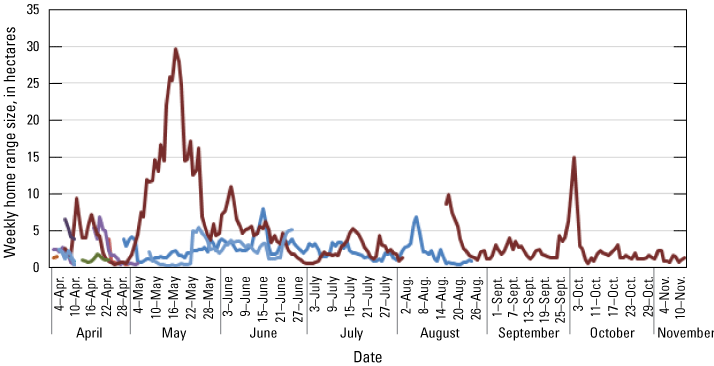
Weekly space use estimates for Yuma Ridgway’s rail in the Salton Sea (California) during 2016 from the 95-percent kernel utilization distribution estimated using kernel methods and a least-squares cross validated smoothing parameter (each line represents a unique individual).
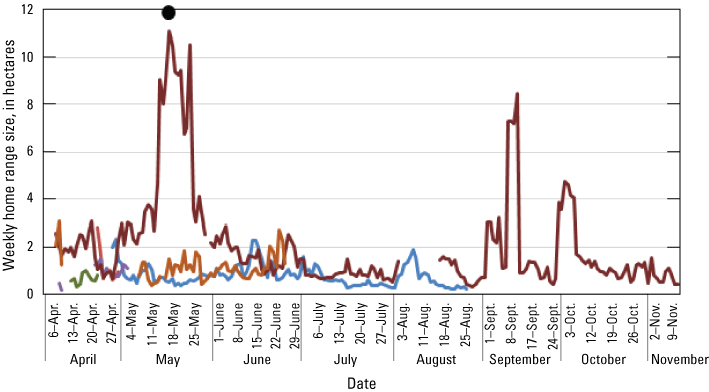
Weekly space use estimates for Yuma Ridgway’s rail in the Salton Sea (California), during 2016, from a utilization distribution estimated using 95-percent local convex hull methods with hulls connecting eight nearest neighbors. Black dot represents a rail with the single greatest home range estimate resulting from relocation upon draining of habitat (each line represents a unique individual).
Kernel estimates of space use showed substantial overlap among individuals total home range (95-percent contours; figs. 26–28). Likewise, core areas (50-percent isopleths) in the Imperial Irrigation District managed marshes showed almost complete overlap among three pairs of individuals, suggesting we had radio-marked mated pairs (fig. 29). The amount of core area overlap among adjacent mated pairs in Salton Sea was approximately the same as observed for pair-bonded Ridgway’s rails in San Francisco Bay. For adjacent unmated rails, by contrast, core area overlap was less in the Salton Sea than in San Francisco Bay (Overton, 2013). One explanation for regional differences in core area overlap is that the tidal environment of San Francisco Bay is much more dynamic on short time scales than within marsh environments of the Salton Sea and requires rails within the bay to move throughout the marsh in response to tidal inundation. Because tidal inundation does not affect rail movement in the Salton Sea, home territoriality and space use can be compressed, resulting in less overlap in core areas and greater population density than within tidal marshes. The area used by rails, in response to changes in habitat, also suggests that tidal marshes in San Francisco Bay that have the most habitat heterogeneity at very local (1 ha or less) scales should require the least amount of movement in response to tidal inundation, which in turn could facilitate greater population density. This pattern of movement related to habitat appears to exist within San Francisco Bay and is consistent with habitat association models developed for rails in that tidal environment (Liu and others, 2012; U.S. Geological Survey, unpub. data, 2015).
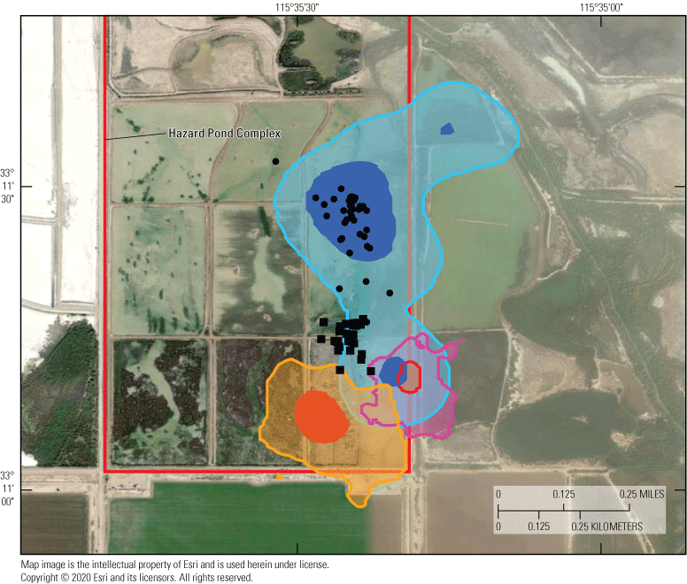
Yuma Ridgway’s rail kernel home range (50 percent and 95 percent isopleths; for birds with >100 relocations, n=3) and individual relocation data (for birds with <100 relocations, n=2) within the Hazard Marshes on Sonny Bono Salton Sea National Wildlife Refuge in 2016. Note: background imagery does not accurately portray vegetation extent during our study. Global Positioning System errors can occur and are assumed to be responsible for isolated locations occurring in unvegetated areas.
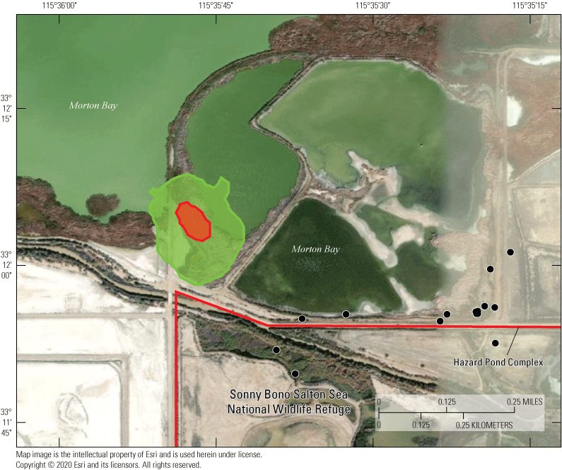
Yuma Ridgway’s rail kernel home range (50-percent and 95-percent isopleths; for birds with >100 relocations, n=1) and individual relocation data (for birds with <100 relocations, n = 1) within Morton Bay adjacent to Sonny Bono Salton Sea National Wildlife Refuge during 2016. Note: background imagery does not accurately portray vegetation extent during our study. Global Positioning System error can occur and are assumed to be responsible for isolated locations occurring in unvegetated areas.
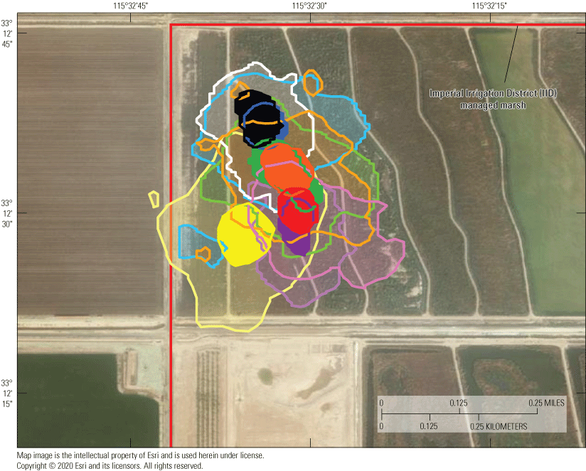
Yuma Ridgway’s rail kernel home range (50-percent and 95-percent isopleths; for birds with >100 relocations, n=7) within the Imperial Irrigation District’s managed marshes near the Salton Sea (California) in 2016. Note: background imagery does not accurately portray vegetation extent during our study. Global Positioning System error may occur and are assumed to be responsible for isolated locations occurring in unvegetated areas.
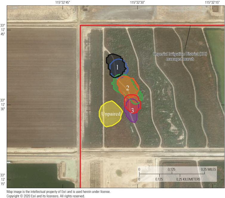
Space use distributions of Yuma Ridgway’s rails captured within the Imperial Irrigation District’s managed marshes near the Salton Sea (California) in 2016 suggest that three sets of mated pairs were radio-marked. Individuals comprising the pair exhibited significant overlap among core space use areas (50-percent kernel isopleths) while maintaining little overlap with adjacent pairs. Numbers indicate the locations of core areas for mated pairs, with each number representing a pair.
Distance between animal relocations can be a useful descriptor of behavioral choices and ecological processes affecting individuals. The maximum distance, or total displacement, between relocations of a single individual ranged between 192 m and 1.7 km, with a mean of 737 m. However, GPS location error is extremely non-normally distributed with nearly exponential error distances in extreme cases and it is impossible to distinguish between temporary extra-territorial movements and most GPS errors. A more robust measure of spatial spread is the distance range for 95 percent of all relocations for an individual. The 95-percent Maximum Displacement Distance (MDD) ranged from 141 to 305 m (mean=228 m), excluding a single outlier (MDD=677 m) with a relatively long tracking history and several territory shifts. Tracking duration ranged from 3 to 126 days (223 days for the outlying individual) and neither total displacement nor 95-percent MDD was affected by tracking duration. These findings indicate that extra-territorial movements are infrequent, but individuals can, and most likely do (despite the occurrence of GPS location error), make substantial movements that range across multiple adjacent territories.
Summary
We performed the first known assessment of relative selenium risk to Yuma Ridgway’s rails occupying unmanaged and managed marshes near the southeastern shoreline of the Salton Sea across a single breeding season (2016). Our results indicated relatively higher risks from dietary selenium exposure for rails occupying unmanaged marshes compared to managed marshes and similar risks among unmanaged marshes (that is, Freshwater [FW] Marsh and Morton Bay). Some consistent “hot spots” for environmental selenium across matrices and sampling periods also were apparent, especially at FW-7. However, risks were potentially elevated for rails occupying the managed Hazard Marshes, where relatively high proportions of Chironomidae and mosquitofish exceeded dietary thresholds for selenium effects on avian reproduction. This pattern was apparent even though Hazard Marshes were sustained by direct (and low selenium) Colorado River water. Previous sampling in these marshes also documented elevated selenium in Chironomidae despite corresponding concentrations of selenium in water and sediments below thresholds of concern (Miles and others, 2009; De La Cruz and others, 2022). Selenium risk, as measured by Chironomidae and mosquitofish, also was elevated in Hazard Marsh HZ9A, which currently receives Colorado River water that is relatively low in selenium. Hazard Marsh HZ9A may undergo future changes in water management (that is, blending of Colorado River water with Alamo River water that is higher in selenium), which could increase already relatively high selenium concentrations in HZ9A. Although the biogeochemical mechanisms driving patterns in selenium concentrations have not been quantified at our sampled sites, Hazard wetlands were created over sediments deposited by the contemporary Salton Sea, yet also received water and sediments from the adjacent Alamo River during floods. This system now has a more closed hydrological flow with emergent vegetation that provides particulates that can enhance selenium bioavailability (Luoma and Presser, 2009).
It is critical to note that one season of sampling is likely insufficient to document the full range of selenium risks to rails in relation to marsh management practices. During 2016, and according to the conditions of the Quantification Settlement Agreement (QSA), mitigation water aimed at slowing the decline in lake elevation (and associated increased salinity) was being delivered to the Salton Sea in the form of lower selenium tail-water runoff from fallowed agricultural fields. However, none of this type of water flowed into Morton Bay through the drainage canals to the east known as the “alphabet laterals.” As of January 2018, mitigation flows have ceased and agricultural producers in Imperial Valley will initiate more stringent water-conservation practices. The ramifications of this change in water management are unknown, but it is possible that the remaining water delivered to drainage canals that sustain unmanaged marshes will have proportionally more selenium laden tile-drain water. Hence, selenium risk to rails, as measured in our study, may not remain constant going forward.
Finally, tradeoffs between selenium risk and limited habitat availability for rails are apparent. The only marshes that appeared to incur consistently low selenium risk to rails were the managed Imperial Irrigation District Marshes, which were created for habitat mitigation in 2009 and 2013 and are 4 kilometers away from the Salton Sea. Due to high levels of territoriality and very limited movement throughout the landscape, the space use patterns exhibited by rails suggest that selenium risk to individuals is not equally shared. Although, we note that rails respond rapidly to changes in habitat availability and quality, as exhibited by one individual that used at least four wetland units during this study; the typical pattern is for rails to be relatively stationary. The one extensively moving individual crossed habitat boundaries as water management practices changed the prevailing habitat condition available to the bird. The selenium risk to this individual is therefore integrated among several, presumably differing, selenium exposures due to its use of a larger landscape. Most individuals do not experience different wetland, habitat, or selenium conditions once territories are established. Behavioral mechanisms, such as regional nomadism, that could mitigate selenium risk by spreading exposure are therefore unlikely to operate. Therefore, limited movement by rails in the Salton Sea could result in population sinks under extreme conditions of selenium toxicity, causing impairment to reproduction or survival in otherwise suitable habitat. The abundance of birds, and therefore the number of individuals susceptible to selenium toxicity, appears to be modestly influenced by large scale habitat availability and less influenced by wetland management or vegetation type. The largest contiguous blocks of habitat are associated with unmanaged marshlands located on the former southeastern shoreline and outside traditional management areas and authorities. Thus, a substantial proportion of the rail population that is using unmanaged marsh on the southeastern shoreline could have disproportionate risk of selenium toxicity. Going forward with the conditions of the QSA and related water management, managed wetlands suitable for rails will likely be highly limited. What remains to be determined definitively is the absolute risk that selenium in these unmanaged (as well as possibly some managed) marshes poses to rail population viability relative to the loss of emergent marsh habitat (managed or unmanaged) as freshwater becomes increasingly limited. Rails could be less sensitive to selenium owing to their evolutionary history of occupying high salinity estuarine environments (Burger and others, 2015; Eddleman and Conway, 202017). However, sublethal effects of selenium exposure concentrations on reproduction and behavior of the species have not been quantified. In the absence of such data, continued hypothesis-driven monitoring of relative rail occupancy and density and concomitant sampling of selenium in likely rail prey items as well as routes of exposure from waterborne, benthic, and epipelagic pathways, is warranted. With advances in telemetry technology, it could be possible, in the future, to track rails year-around and evaluate behavioral, survival, and reproductive rates between managed versus unmanaged marsh and across the selenium concentration gradient. Such detailed information could allow accurate assessment of future rail population viability and help support management of marsh and Yuma Ridgway’s rails at Salton Sea.
References Cited
Ackerman, J.T., and Eagles-Smith, C.A., 2010, Agricultural wetlands as potential hotspots for mercury bioaccumulation—Experimental evidence using caged fish: Environmental Science & Technology, v. 44, no. 4, p. 1451–1457. [Available at https://doi.org/10.1021/es9028364.]
Ackerman, J.T., Overton, C.T., Casazza, M.L., Takekawa, J.Y., Eagles-Smith, C.A., Keister, R.A., and Herzog, M.P., 2012, Does mercury contamination reduce body condition of endangered California clapper rails?: Environmental Pollution, v. 162, p. 439–448. [Available at https://doi.org/10.1016/j.envpol.2011.12.004.]
Albertson, J.D., 1995, Ecology of the California clapper rail in the south San Francisco Bay: San Francisco, Calif., San Francisco State University, Master thesis, 216 p., accessed December 15, 2019, at https://www.researchgate.net/publication/34061656_Ecology_of_the_California_Clapper_Rail_in_South_San_Francisco_Bay_MA_thesis/link/00b7d5314c903441e1000000/download.
Barnum, D.A., Bradley, T., Cohen, M., Wilcox, B., and Yanega, G., 2017, State of the Salton Sea—A science and monitoring meeting of scientists for the Salton Sea: U.S. Geological Survey Open-File Report 2017–1005, 20 p., accessed December 15, 2019, at https://doi.org/10.3133/ofr20171005.
Battin, J., 2004, When good animals love bad habitats—Ecological traps and the conservation of animal populations: Conservation Biology, v. 18, no. 6, p. 1482–1491. [Available at https://doi.org/10.1111/j.1523-1739.2004.00417.x.]
Bui, T.V.D., Takekawa, J.Y., Overton, C.T., Schultz, E.R., Hull, J.M., and Casazza, M.L., 2015, Movements of radio-marked California Ridgway’s rails during monitoring surveys—Implications for population monitoring: Journal of Fish and Wildlife Management, v. 6, no. 1, p. 227–237. [Available at https://doi.org/10.3996/092014-JFWM-069.]
Burger, J., Tsipoura, N., Niles, L.J., Gochfeld, M., Dey, A., and Mizrahi, D., 2015, Mercury, lead, cadmium, arsenic, chromium and selenium in feathers of shorebirds during migrating through Delaware Bay, New Jersey—Comparing the 1990s and 2011/2012: Toxics, v. 3, no. 1, p. 63–74. [Available at https://doi.org/10.3390/toxics3010063.]
Byron, E.R., and Ohlendorf, H.M., 2007, Diffusive flux of selenium between lake sediment and overlying water—Assessing restoration alternatives for the Salton Sea: Lake and Reservoir Management, v. 23, no. 5, p. 630–636. [Available at https://doi.org/10.1080/07438140709354042.]
Calenge, C., 2006, The package “adehabitat” for the R software—A tool for the analysis of space and habitat use by animals: Ecological Modelling, v. 197, no. 3–4, p. 516–519. [Available at https://doi.org/10.1016/j.ecolmodel.2006.03.017.
California Resources Agency, 2007, Salton Sea ecosystem restoration program final programmatic environmental impact report: California Department of Water Resources, accessed December 15, 2019, at https://water.ca.gov/saltonsea.
Casazza, M.L., Ricca, M.A., Overton, C.T., Takekawa, J.Y., Merritt, A.M., and Ackerman, J.T., 2014, Dietary mercury exposure to endangered California clapper rails in San Francisco Bay: Marine Pollution Bulletin, v. 86, no. 1–2, p. 254–260, [Available at https://doi.org/10.1016/j.marpolbul.2014.07.009.]
Case, H.L.I., Boles, J., Delgado, A., Nguyen, T., Osugi, D., Barnum, D.A., Decker, D., Steinberg, St., Steinberg, Sh., Keene, C., White, K., Lupo, T., Gen, S., and Baerenklau, K.A., 2013, Salton Sea ecosystem monitoring and assessment plan: U.S. Geological Survey Open-File Report 2013–1133, 220 p., accessed December 15, 2019, at https://doi.org/10.3133/ofr20131133.
Conway, C.J., 2011, Standardized North American marsh bird monitoring protocol: Waterbirds, v. 34, no. 3, p. 319–346. [Available at https://doi.org/10.1675/063.034.0307.]
Conway, C.J., Eddleman, W.R., Anderson, S.H., and Hanebury, L.R., 1993, Seasonal changes in Yuma clapper rail vocalization rate and habitat use: The Journal of Wildlife Management, v. 57, no. 2, p. 282–290. [Available at https://doi.org/10.2307/3809425.]
De La Cruz, S.E., Woo, I., Miles, A.K., Ricca, M.A., Antonino, C.Y., and Hall, L.A., 2022, Biological tissue data used to evaluate selenium hazards in the Salton Sea ecosystem (1984–2020): U.S. Geological Survey data release, https://doi.org/10.5066/P9ECP7O0.
Eddleman, W.R. and Conway, C.J., 2020, Ridgway's Rail (Rallus obsoletus), ver. 1.0, in Rodewald, P.G., ed., Birds of the World: Ithaca, NY, Cornell Lab of Ornithology. [Available at https://doi.org/10.2173/bow.ridrai1.01.]
Fan, T.W.M., Teh, S.J., Hinton, D.E., and Higashi, R.M., 2002, Selenium biotransformations into proteinaceous forms by foodweb organisms of selenium-laden drainage waters in California: Aquatic Toxicology (Amsterdam, Netherlands), v. 57, no. 1–2, p. 65–84. [Available at https://doi.org/10.1016/S0166-445X(01)00261-2.]
Fiske, I., and Chandler, R., 2011, unmarked—An R package for fitting hierarchical models of wildlife occurrence and abundance: Journal of Statistical Software, v. 43, no. 10, p. 1–23. [Available at https://doi.org/10.18637/jss.v043.i10.]
García-Fernández, A.J., Espín, S., and Martínez-López, E., 2013, Feathers as a biomonitoring tool of polyhalogenated compounds—A review: Environmental Science & Technology, v. 47, no. 7, p. 3028–3043. [Available at https://doi.org/10.1021/es302758x.]
Getz, W.M., and Wilmers, C.C., 2004, A local nearest‐neighbor convex‐hull construction of home ranges and utilization distributions: Ecography, v. 27, no. 4, p. 489–505. [Available at https://doi.org/10.1111/j.0906-7590.2004.03835.x.
Groover, K.D., Roberts, S.A., McPherson, J.W., and Rosen, M.R., 2022, Water and sediment data used to evaluate selenium hazards in the Salton Sea ecosystem: U.S. Geological Survey data release, https://doi.org/10.5066/P9VIK7LK.
Hamilton, S.J., 2004, Review of selenium toxicity in the aquatic food chain: The Science of the Total Environment, v. 326, no. 1–3, p. 1–31. [Available at https://doi.org/10.1016/j.scitotenv.2004.01.019.]
Harrity, E.J., and Conway, C.J., 2020, Satellite transmitters reveal previously unknown migratory behavior and wintering locations of Yuma Ridgway’s Rails: Journal of Field Ornithology, v. 91, no. 3, p. 300–312. [Available at https://doi.org/10.1111/jofo.12344.]
Harrity, E.J., Stevens, B.S., and Conway, C.J., 2020, Keeping up with the times—Mapping range-wide habitat suitability for endangered species in a changing environment: Biological Conservation, v. 250, 10 p. [Available at https://doi.org/10.1016/j.biocon.2020.108734.]
Lemly, A.D., 2004, Aquatic selenium pollution is a global environmental safety issue: Ecotoxicology and Environmental Safety, v. 59, no. 1, p. 44–56. [Available at https://doi.org/10.1016/S0147-6513(03)00095-2.]
Lemly, A.D., and Ohlendorf, H.M., 2002, Regulatory implications of using constructed wetlands to treat selenium-laden wastewater: Ecotoxicology and Environmental Safety, v. 52, no. 1, p. 46–56. [Available at https://doi.org/10.1006/eesa.2002.2145.]
Lichti, N.I., and Swihart, R.K., 2011, Estimating utilization distributions with kernel versus local convex hull methods: The Journal of Wildlife Management, v. 75, no. 2, p. 413–422. [Available at https://doi.org/10.1002/jwmg.48.]
Liu, L., Wood, J., Nur, N., Salas, L., and Jongsomjit., D., 2012, California clapper rail (Rallus longirostris obsoletus) population monitoring—2005–2011: Petaluma, Calif., Point Reyes Bird Observatory Conservation Science, Final technical report, 81 p., accessed April 17, 2022, at https://spartina.org/documents/CLRA2005-11FinalReportPRBO_Web.pdf.
Luoma, S.N., and Presser, T.S., 2009, Emerging opportunities in management of selenium contamination: Environmental Science & Technology, v. 43, no. 22, p. 8483–8487. [Available at https://doi.org/10.1021/es900828h.]
MacDonald, G.M., 2010, Water, climate change, and sustainability in the southwest: Proceedings of the National Academy of Sciences of the United States of America, v. 107, no. 50, p. 21256–21262. [Available at https://doi.org/10.1073/pnas.0909651107.]
McKernan, M.A., Reynolds, K.D., and Takekawa, J.Y., 2016, Final environmental contaminants program on-refuge investigations sub-activity—AZ, CA—Selenium exposure to Yuma clapper rails (Rallus longirostris yumanensis) inhabiting the lower Colorado River and the Salton Sea: Department of the Interior, U.S. Fish and Wildlife Service Region 2 Report.
Miles, A.K., Ricca, M.A., Meckstroth, A., and Spring, S.E., 2009, Salton Sea ecosystem monitoring project: U.S. Geological Survey Open-File Report 2009–1276, 150 p., accessed December 15, 2019, at https://doi.org/10.3133/ofr20091276.
Ohlendorf, H.M., 1999, Selenium was a time bomb: Human and Ecological Risk Assessment, v. 5, no. 6, p. 1181–1185. [Available at https://doi.org/10.1080/10807039.1999.10518885.]
Ohlendorf, H.M., 2002, The birds of Kesterson Reservoir—A historical perspective: Aquatic Toxicology (Amsterdam, Netherlands), v. 57, no. 1–2, p. 1–10. [Available at https://doi.org/10.1016/S0166-445X(01)00266-1.]
Overton, C.T., Casazza, M.L., Takekawa, J.Y., Strong, D.R., and Holyoak, M., 2014, Tidal and seasonal effects on survival rates of the endangered California clapper rail—Does invasive Spartina facilitate greater survival in a dynamic environment?: Biological Invasions, v. 16, no. 9, p. 1897–1914. [Available at https://doi.org/10.1007/s10530-013-0634-5.]
Overton, C.T., Ricca, M.A., Anderson, T.W., Merritt, A., Harrity, E., Matchett, E., and Casazza, M.L., 2022, Yuma Ridgway’s rail (Rallus obsoletus yumanensis) population surveys, rail movement, and potential habitat at the Salton Sea of California: U.S. Geological Survey data release, https://doi.org/10.5066/P9JRP0L6.
Presser, T.S., and Luoma, S.N., 2010, A methodology for ecosystem‐scale modeling of selenium: Integrated Environmental Assessment and Management, v. 6, no. 4, p. 685–710. [Available at https://doi.org/10.1002/ieam.101.]
R Development Core Team, 2017, R—A language and environment for statistical computing: R Foundation for Statistical Computing, Vienna, Austria, accessed December 15, 2019, at http://www.R-project.org.
Ricca, M.A, Overton, C.T., Anderson, T.W., Merritt, A., Harritty, E. Matchett, E., and Casazza, M.L., 2022, Selenium concentrations in Yuma Ridgway's Rails occupying managed and unmanaged emergent marshes at the Salton Sea: U.S. Geological Survey data release, https://doi.org/10.5066/P9R39F33.
Royle, J.A., 2004, N‐mixture models for estimating population size from spatially replicated counts: Biometrics, v. 60, no. 1, p. 108–115. [Available at https://doi.org/10.1111/j.0006-341X.2004.00142.x.]
Sabo, J.L., Sinha, T., and Bowling, L.C., Schoups, G.H.W., Wallender, W.W., Campana, M.E., Cherkauer, K.A., Fuller, P.L., Graf, W.L., Hopmans, J.W., Kominoski, J.S., Taylor, C., Trimble, S.W., Webb, R.H., and Wohl, E.E., 2010, Reclaiming freshwater sustainability in the Cadillac Desert: Proceedings of the National Academy of Sciences, v. 107, p. 21263–21269. [Available at https://doi.org/10.1073/pnas.1009734108.]
Saiki, M.K., Martin, B.A., and May, T.W., 2010, Final report—Baseline selenium monitoring of agricultural drains operated by the Imperial Irrigation District in the Salton Sea Basin: U.S. Geological Survey Open-File Report 2010–1064, 100 p., accessed December 15, 2019, at https://doi.org/10.3133/ofr20101064.
Saiki, M.K., Martin, B.A., and May, T.W., 2012, Selenium in aquatic biota inhabiting agricultural drains in the Salton Sea Basin, California: Environmental Monitoring and Assessment, v. 184, no. 9, p. 5623–5640. [Available at https://doi.org/10.1007/s10661-011-2367-1.]
Schroeder, R.A., Orem, W.H., and Kharaka, Y.K., 2002, Chemical evolution of the Salton Sea, California—Nutrient and selenium dynamics: Hydrobiologia, v. 473, no. 1, p. 23–45. [Available at https://doi.org/10.1023/A:1016557012305.]
Seiler, R., Skorupa, J., and Peltz, L., 1999, Areas susceptible to irrigation-induced selenium contamination of water and biota in the western United States: U.S. Geological Survey Circular 1180, 36 p. [Available at https://doi.org/10.3133/cir1180.]
Shuford, W.D., Warnock, N., Molina, K.C., and Sturm, K.K., 2002, The Salton Sea as critical habitat to migratory and resident waterbirds: Hydrobiologia, v. 473, no. 1/3, p. 255–274. [Available at https://doi.org/10.1023/A:1016566709096.
U.S. Environmental Protection Agency, 2016, Aquatic life ambient water quality criterion for Selenium—Freshwater: Office of Water, U.S. Environmental Protection Agency, 807 p. [Available at https://www.epa.gov/sites/production/files/2016-07/documents/aquatic_life_awqc_for_selenium_-_freshwater_2016.pdf.]
U.S. Fish and Wildlife Service, 2014c, Sonny Bono Salton Sea NWRC Final Comprehensive Conservation Plan: U.S. Fish and Wildlife Service, accessed December 15, 2019, at https://www.fws.gov/refuge/Sonny_Bono_Salton_Sea/what_we_do/planning.html.
Worton, B.J., 1989, Kernel methods for estimating the utilization distribution in home‐range studies: Ecology, v. 70, no. 1, p. 164–168. [Available at https://doi.org/10.2307/1938423.]
Conversion Factors
International System of Units to U.S. customary units
Datum
Horizontal coordinate information is referenced to the North American Datum of 1983 (NAD 83).
Data initially recorded in World Geodetic System of 1984 (WGS 84) were projected to NAD 83.
Supplemental Information
Selenium concentrations for all water samples were recorded on a wet weight (ww) basis as parts per billion (ppb), and all tissue samples (other than blood) on a dry weight (dw) basis as part per million (ppm). Units in ppb or ppm are equivalent to micrograms per liter (μg/L) and micrograms per gram (μg/g), respectively, which are used in the reporting of results for selenium concentrations herein. Selenium concentrations in whole blood are reported as μg/g, ww. Estimated body burden of selenium in crayfish is reported as the product of whole-body dry weight mass and dry weight selenium concentration (Ackerman and Eagles-Smith, 2010). Average whole-body dry weight mass was used to estimate body burden of selenium for composited small crayfish samples. Concentration data are available at https://doi.org/10.5066/P9R39F33 and data for Yuma Ridgway’s rail call count surveys, movement (GPS relocation), and remotely sensed potential habitat are available at https://doi.org/10.5066/P9JRP0L6, for the Salton Sea, California, 2016.
Abbreviations
ACF
Analytical Control Facility
AIC
Akaike information criterion
dw
dry weight
EPA
U.S. Environmental Protection Agency
FW
Freshwater
GPS
Global Positioning System
HZ
Hazard Marsh
HDPE
high-density polyethylene
IID
Imperial Irrigation District
Landsat
land satellite
LoCoH-k
local convex hulls
MB
Morton Bay
MDD
maximum displacement distance
NIST
National Institute of Standards and Technology
nfw
sample size for Freshwater Marsh
nhz
sample size for Hazard Marsh complex
niid
sample size for Imperial Irrigation District complex
nmb
sample size for Morton Bay
NAMBMP
North American Marsh Bird Monitoring Protocol
QA/QC
quality assurance/quality control
QSA
Quantification Settlement Agreement
SBSSNWR
Sonny Bono Salton Sea National Wildlife Refuge
SD
standard deviation
SE
standard error
TERL
Trace Element Research Lab
USFWS
U.S. Fish and Wildlife Service
USGS
U.S. Geological Survey
ww
wet weight
For more information concerning the research in this report, contact the
Director, Western Ecological Research Center
U.S. Geological Survey
3020 State University Drive East
Sacramento, California 95819
https://www.usgs.gov/centers/werc
Publishing support provided by the U.S. Geological Survey Science Publishing Network, Sacramento Publishing Service Center
Suggested Citation
Ricca, M.A., Overton, C.T., Anderson, T.W., Merritt, A., Harrity, E., Matchett, E., and Casazza, M.L., 2022, Yuma Ridgway’s rail selenium exposure and occupancy within managed and unmanaged emergent marshes at the Salton Sea: U.S. Geological Survey Open-File Report 2022–1045, 49 p., https://doi.org/10.3133/ofr20221045.
ISSN: 2331-1258 (online)
Study Area
| Publication type | Report |
|---|---|
| Publication Subtype | USGS Numbered Series |
| Title | Yuma Ridgway’s rail selenium exposure and occupancy within managed and unmanaged emergent marshes at the Salton Sea |
| Series title | Open-File Report |
| Series number | 2022-1045 |
| DOI | 10.3133/ofr20221045 |
| Year Published | 2022 |
| Language | English |
| Publisher | U.S. Geological Survey |
| Publisher location | Reston, VA |
| Contributing office(s) | Western Ecological Research Center |
| Description | Report: x, 49 p.; 2 Data Releases |
| Country | United States |
| State | California |
| Other Geospatial | Salton Sea |
| Online Only (Y/N) | Y |
| Google Analytic Metrics | Metrics page |