

Potential Effects of Sea Level Rise on Nearshore Habitat Availability for Surf Smelt (Hypomesus pretiosus) and Eelgrass (Zostera marina), Puget Sound, Washington
Links
- Document: Report (21.9 MB pdf) , HTML , XML
- Data Release: USGS data release — Data collected in 2010 to evaluate habitat availability for surf smelt and eelgrass in response to sea level rise on Bainbridge Island, Puget Sound, Washington State, USA
- Download citation as: RIS | Dublin Core
Abstract
In this study we examine the potential effects of three predicted sea level rise (SLR) scenarios on the nearshore eelgrass (Zostera marina L.) and surf smelt (Hypomesus pretiosus) spawning habitats along a beach on Bainbridge Island, Washington. Baseline bathymetric, geomorphological, and biological surveys were conducted to determine the existing conditions at the study site. The results of these surveys were coupled with a predictive model that estimates SLR-induced changes to coastal ecosystems based upon local topography and land-cover data. This model simulates the changes in nearshore habitat through time. The model inputs for SLR are probable values reported by the Intergovernmental Panel on Climate Change, and by user-defined values. The predicted effects of SLR are presented as (1) habitat type change and (2) the graphic response of developed dry land depicting the influence of shoreline armoring. This report describes the geophysical and biological characteristics at the Bainbridge Island study site, the modeling methods used to produce depictions of habitat changes, and a possible decrease in surf smelt spawning and an increase in eelgrass habitat availability in response to increases in sea level.
Introduction
Evidence suggests that sea level rise (SLR) will impose impacts on virtually all intertidal ecosystems (Intergovernmental Panel on Climate Change [IPCC], 2019). Examples of these impacts include, but are not limited to, coastal recession, beach scour, sediment coarsening, beach narrowing, and steepening of beach slope (Bird, 1993; Leatherman, 2001; Ranasinghe and others, 2012; Raymond and others, 2018). Projections for SLR on the Pacific coast of North America range from 0.15 to 1.6 meters (m) by 2100 (National Resource Council, 2012). In the Puget Sound, the effects of SLR along about 4,000 kilometers (km) of coastline suggest that the effects could be relatively widespread in the nearshore areas. The probability of vertical and horizontal beach impacts caused by such increases in water level has raised questions and concerns about potential deleterious effects upon nearshore species that occupy these habitats.
Nearshore areas in the Puget Sound have been identified by the Puget Sound Partnership (PSP) as important for protection and restoration to support ecosystem recovery efforts (PSP, 2008). Two valued ecosystem components of the nearshore environment are the spawning areas used by beach-spawning forage fishes, and eelgrass (Zostera sp.) beds used as fish nursery areas. Adult surf smelt (Hypomesus pretiosus) aggregate in the upper intertidal zone along the shoreline and broadcast their (approximately 1-mm diameter) adhesive eggs onto sand-gravel mix beach sediments just below the waterline during high tides. Surf smelt eggs then remain on the beach while incubation occurs (Penttila, 2007). Juvenile forage fish have been observed and captured in eelgrass beds, which indicates the use of this habitat for rearing (Johnson and others, 2008). Eelgrass, which is restricted to nearshore areas (< 10 m in depth), has deteriorated in condition and decreased in distribution in the Puget Sound (Mumford, 2007). The upper limit of eelgrass distribution is constrained by risk of desiccation (in the intertidal zone) and its lower limit is set by light penetration (Mumford, 2007). Potentially, SLR will affect the distribution of eelgrass by truncating the lower limit. If shoreline armoring is present, the upper limit of the grass also might be truncated because the eelgrass bed cannot expand upslope as water levels rise. However, if suitable substrate is present, eelgrass could expand upslope in the absence of shoreline armoring. Surf smelt have been recognized by regional entities such as the PSP and the Puget Sound Ecosystem Monitoring Program (PSEMP) as species of interest because of the recent decline in population levels of many more charismatic species at higher trophic levels (for example, seabirds, salmon, and orca; Mumford, 2007; Penttila, 2007; PSP, 2008). The PSP and PSEMP have recognized the high priority for eelgrass protection and restoration because of the cultural and ecological value of eelgrass and its connection to other species of concern, such as Pacific sand lance (Ammodytes personatus) and salmon (Oncorhynchus spp.). Furthermore, federal legislation enacted through the Clean Water Act 404(b)(1) (40 CFR 230) (1972) and the Magnuson-Stevens Fishery Conservation and Management Reauthorization Act (P.L. 109-479) (2006) requires mitigating or avoiding adverse impacts to habitats that support eelgrass within U.S. territorial waters.
Throughout the Puget Sound, extensive shoreline armoring has been constructed to prevent the landward encroachment of the sea. These shoreline modifications are designed to dissipate wave energy, maintain navigation channels, and prevent shoreline erosion, and they commonly include bulkheads, rip-rap, seawalls, jetties, and breakwaters (Williams and Thom, 2001). Nearshore habitats in the Puget Sound are likely to undergo significant changes owing to SLR because of the combined effects of deeper water and the likely response by landowners to increase shoreline armoring. The narrowing of the nearshore environment is expected as public and private entities could respond to SLR with armoring and construction of bulkheads to protect property and infrastructure (Titus, 1998; Mitsova and Esnard, 2012). Where shoreline armoring is lacking, the process of change in response to SLR will be unconstrained, and erosion and deposition associated with natural processes will modify the shoreline and alter the existing habitat. Where armoring currently exists or might be constructed in response to the threat of SLR, the change process would be constrained, and the outcome would be a narrowing or “squeeze” between SLR and stable-armored shorelines. Under the narrowing scenario, beaches used by surf smelt will be squeezed, resulting in a reduction in the habitat available for spawning (IPCC, 2007; Krueger and others, 2010). Even apart from the effects of SLR, armoring can affect spawning habitat by physical burial of the upper intertidal zone through the addition of armoring materials, or separation from feeder bluffs that nourish beaches, which in turn leads to coarsening of the beach substrate and lowering of the beach elevation (Williams and Thom, 2001). Furthermore, as the nearshore area is narrowed, eelgrass distribution will be reduced as the deepest margins are exposed to reduced light levels, and expansion upslope is restricted by armoring. Reduced eelgrass distribution then impacts surf smelt by limiting or shrinking feeding and rearing habitats. Some investigators have already suggested that rising water levels and water temperatures that would accompany predicted climate change could negatively affect eelgrass in the Northwest (Short and Neckles, 1999; Thom and others, 2005), as has been documented in eelgrass beds within Chesapeake Bay in the northeastern U.S. (Najjar and others, 2010; Bilkovic and others, 2019).
Model simulations of habitat change can provide important insights into how climate change and SLR could affect local habitats and shoreline-dependent organisms (Galbraith and others, 2002; Craft and others, 2009; Fuentes and others, 2010). In addition, SLR modeling is being used to predict ecological and societal actions in response to the effects of climate change (Lentz and others, 2015), beach overwash (Plant and others, 2014), infrastructure vulnerabilities (Donoghue and others, 2013), and landowner response to rising sea levels (McNamara and Keeler, 2013). To study the potential effects of SLR on the nearshore, we used the Sea Level Affecting Marshes Model (SLAMM; Clough and others, 2010) to simulate changes in landcover through time and under different SLR scenarios. The SLAMM model, in concert with local land-cover and topographic data, has been used throughout the coastal Pacific Northwest to forecast SLR impacts to estuarine habitats and coastal communities (Park and others, 1993; Glick and others, 2007; Clough and Larson, 2010).
The objectives of the study described in this report were to: (1) inventory existing habitat conditions, including surf smelt spawning locations, extent of eelgrass beds, beach morphology, and shoreline armoring attributes; (2) predict SLR using SLAMM, and use these projections to illustrate potential habitat alterations caused by SLR for the years 2050 and 2100; and (3) compare physical attributes and surf smelt spawning-site selection on adjacent beaches with different land-use characteristics. Using these objectives, we hypothesized that both eelgrass and surf smelt spawning habitat would be reduced with increasing SLR, with the greatest amount of reduction occurring along the developed shoreline. Associated biological variables showing surf smelt spawning presence, geological variables describing beach composition, sample locations, and modeling data for this publication are in Tomka and others (2020).
Methods
Description of Study Area
Two study sites in central Puget Sound, Washington (fig. 1) were selected to sample a suite of biological, hydrological, and geological variables. These sites, on the northern tip of Bainbridge Island (fig. 2), lie adjacent to each other, but have different land-use characteristics. The first study site, Fay Bainbridge Park, is a 6.8-hectare general-use Bainbridge Island Metropolitan Parks and Recreation District Park, with approximately 430 m of undeveloped shoreline. The coastline is an estuarine accretion beach with a backshore berm containing an accumulation of large woody debris, and the shoreline is not armored. The upland habitat is a lowland that contains a grass lawn, paved roadways and parking areas, and park shelters that abut a forested upland. The second study site, Point Monroe, lies immediately north of Fay Bainbridge Park. Point Monroe is an approximately 1-km long residentially developed, recurved spit constructed from fill (Williams and others, 2004) and an accretion beach seaward, and the site forms a tidal lagoon landward. The seaward-facing aspect of the spit is largely devoid of terrestrial vegetation, with shoreline armoring along most of the developed beachfront.
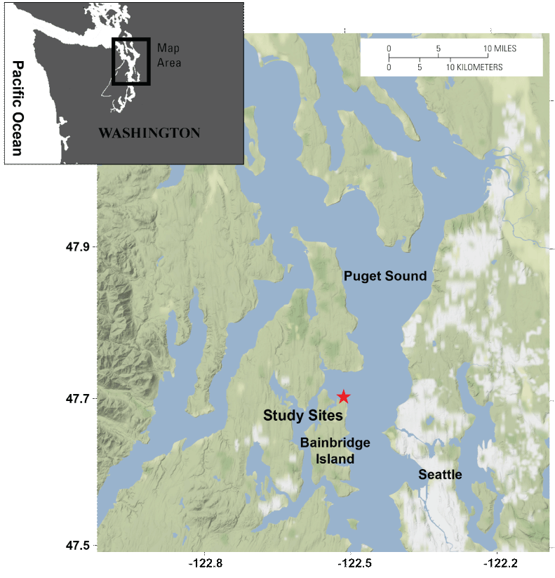
Central Puget Sound, Washington State. The location of the two study sites is indicated by the red star (see fig. 2). Base map tiles by Stamen Design, under CC BY 3.0; base map data by OpenStreetMap, under ODbL. [km, kilometer.]
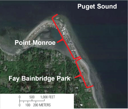
The two study sites, Fay Bainbridge Park and Point Monroe, Bainbridge Island, Washington. The base map is U.S. Geological Survey High Resolution Orthoimagery, 0.5-meter (m) resolution, 2010.
Benthic substrates at both study sites are classified as mixed-sediment, with a gravel foreshore and a sandy low-tide terrace (Pontee and others, 2004). Intertidal and subtidal vegetation observed at both sites includes primarily patchy and contiguous beds of the native eelgrass (Zostera marina L.), along with scattered patches of bull kelp (Nereocystis luetkeana), and seaweed (Ulva sp., Gracilariopsis sp.). At the time of survey, the non-native eelgrass Z. japonica was not directly observed at these sites, but it is possible that it could have been interspersed within or near the beds of Z. marina. Shoot densities of eelgrass beds at Fay Bainbridge Park (1,143±475 shoots per square meters [m2]) were about twofold greater than the eelgrass beds at Point Monroe (507±479 shoots per m2; R. Takesue, U.S. Geological Survey, written commun., 2012). These eelgrass-shoot densities are high but consistent with those in eelgrass beds at other central Puget Sound locations. Additionally, forage fish spawning surveys previously conducted near this study site indicate that these beaches could provide favorable spawning habitat for surf smelt (Penttila, 2001).
Study Methods
Bathymetric and Eelgrass Mapping
Detailed data on bathymetry and eelgrass distribution were simultaneously collected using a single beam echosounder system. The system consisted of a Biosonics 420 kilohertz (6° beam angle) transducer and deck unit, a data acquisition laptop PC, and Trimble real-time kinematic global positioning system (RTK-GPS). For a complete description of the acoustic survey system, see Stevens and others (2008). Cross-shore survey transect lines were spaced at 25-m intervals along the 3-km stretch of the study area and were followed from as close to shore as possible to a depth of 20 m. Cross-shore survey data were supplemented with several additional along-shore lines that roughly followed bathymetric contours.
Acoustic data were analyzed using a custom graphical user interface that implements a signal processing algorithm (Sabol and others, 2002) that is applied to each sonar sounding to extract the location of the bottom and presence of vegetation (Stevens and others, 2008; Depew and others, 2009). Individual acoustic returns along a survey line were grouped into packets of 10, and eelgrass percentage cover was calculated as the fractional percentage of acoustic returns that were classified as vegetated within each group, resulting in an estimate of eelgrass percentage cover every 4 to 5 m (depending on the vessel speed). Eelgrass percentage cover measurements were interpolated onto a grid with 5-m resolution using kriging (Davis, 2002).
Topographic elevation measurements were collected on foot during low tide using the RTK-GPS mounted on backpacks. Bathymetric and topographic data were merged, and linear interpolation was used to produce a representing the surface topography and nearshore bathymetry. The survey-grade global positioning system (GPS) equipment used in this project have manufacturer-reported root-mean-square accuracies of approximately ±3 centimeters (cm) + 2 parts per million of baseline length (typically 10 km or less) in the horizontal and approximately ±5 cm + 2 parts per m in the vertical while operating in real-time kinematic surveying mode (Trimble Navigation Limited, 1998). These reported accuracies are, however, additionally subject to multi-path, satellite obstructions, poor satellite geometry, and atmospheric conditions that can combine to cause a vertical GPS drift that can be as much as 10 cm (Sallenger and others, 2003). While repeatability tests and merges with topographic data collected with a backpack RTK-GPS suggest sub-decimeter vertical accuracy, significant variability in seawater temperature (about 10 degrees Celsius) and salinity can affect depth estimates by as much as 20 cm in 12 m of water. Therefore, a conservative estimate of the total vertical uncertainty for these nearshore bathymetry measurements is approximately 0.15 m.
Surf Smelt Spawning Surveys
Field Sampling
Spawning surveys were conducted October 20-21, 2010, coinciding with the local historical surf smelt spawning season (Schaefer, 1936; Penttila, 2000). To select beach areas for sampling, the northeast-facing shoreline that extended the length of the study area was divided into 30-m segments using ArcView GIS (version 3.3, Environmental Systems Research Institute Inc., Redlands, California, USA). The 30-m segment was selected as the base unit for sampling based on forage fish sampling protocols of Moulton and Penttila, (2001). The sampling reaches consisted of approximately 510 m of shoreline at Point Monroe and approximately 430 m along Fay Bainbridge Park. Random subsets of seven beach segments at Point Monroe and seven beach segments at Fay Bainbridge Park were selected for sampling.
Beach segments were sampled when tides were lower than 2.1 m above Mean Lower Low Water (MLLW), when the nearshore intertidal portion of the beach was exposed. At each beach segment, we recorded beach and beach armoring attributes. The location of each sample point, and the positions of shoreline armoring (if present) were recorded with GPS. Owing to the difficulty of observing the small (1 mm) surf smelt eggs in the field, beach sediments were collected for laboratory-based egg search and enumeration efforts. At each beach segment, 12 sediment samples were collected using both transect and random location approaches. Sediment collection by the transect approach was modeled after Moulton and Penttila (2001), and four samples of beach material (500 milliliters [mL] each) were collected along a transect line positioned at 2.4 m above MLLW elevation. One site (Site 13) had shoreline armoring present at 2.26 m above MLLW, and the transect line was positioned in sediment at the base of the armoring. For the random sample location approach, 500 mL samples were collected from randomly selected sample locations from a 1-m grid overlay of the exposed beach area. At each substrate sample location (transect and random), a plastic scoop was used to collect 500 ml of the top 3 cm of beach sediment. Samples were then transferred to 500 mL plastic jars. Stockard’s solution (85 percent water, 6 percent glycerin, 5 percent formalin and 4 percent glacial acetic acid) was added to the collected beach material to preserve any eggs that were included in the sample for further laboratory analysis. Also, at each substrate sample location, an additional 250 ml of beach sediment was collected for subsequent grain-size analysis.
Laboratory Processing of Sample
Within the laboratory, small fractions of preserved beach sediment samples were transferred to 8-cm diameter Petri dishes. Enough water to cover the sediment was added to each Petri dish to facilitate viewing. Samples were examined under a dissecting microscope (10 to 20 ×) for counts of total, viable, and dead surf smelt eggs. If surf smelt eggs were present, the first 50 eggs were removed from the sample and preserved with Stockard’s solution, and any remaining eggs were enumerated. Eggs were considered viable if their shells appeared translucent and were considered dead if they were opaque (Rice, 2006). Ruptured eggshells with no intact embryo were not counted.
Grain-Size Analysis
Sediment samples that were collected for grain-size analysis were desiccated at 60 degrees C for 48 hours in a drying oven. Sediment size and composition were determined by standard dry sieving techniques (Folk and Ward, 1957) using test sieves and a Meinzer II sieve shaker. Physical analysis of sediment size and composition was calculated using GRADISTAT (Version 6.0; Blott and Pye, 2001). Statistical parameters for grain size were calculated by the Folk and Ward (1957) graphical method, and qualitative description of the dominant sediment size at each sample site was classified according to the Udden-Wentworth scale (Udden, 1914; Wentworth, 1922). To document the physical properties of the sediment at each of the sample locations, we calculated grain size and composition properties. The following variables were used to describe the sediments: sediment grain size (in phi), grain size sorting, skewness, and kurtosis. To test for differences in sediments and spawning between Fay Bainbridge Park and Point Monroe, an analysis of variance (ANOVA) was used to determine the significance of the differences. Statistical analyses were carried out using R software (R Core Team, 2014). A significance level of α = 0.05 was used for all tests.
Modeling Habitat Selection for Spawning
Owing to the relatively small sampling area and the adjacent nature of the samples, the influence of spatial autocorrelation among sites was examined for the presence of eggs using the ‘ape’ package and R software (R Core Team, 2014). Associations of surf smelt eggs with beach characteristics were evaluated using logistic regression (generalized linear model binomial distribution with logit link) on presence/absence egg data using R software. The response variable (egg presence) was coded 0–1 (absence-presence) as was the covariate armoring. Our full model included covariates: (1) grain size (in mm), (2) grain sorting, (3) gravel percentage, (4) sand percentage, (5) armoring, (6) elevation (in m above MLLW), and (7) beach slope percentage. We used Akaike’s information criterion (AIC) to judge the fit of candidate model subsets to the data over a range of model subsets extending from a null model (intercepts only) to a full model whereby all covariates were included (Burnham and Anderson, 2002; Zuur and others, 2009). Our candidate model subsets were chosen by using a simple stepwise backwards removal procedure, whereby individual variables were dropped from the full model, and the relative change in AIC value was used to determine the relative importance of the variable to the model.
Sea Level Rise Modeling
The effect of SLR on shorelines and tidal habitats within our study area was modeled using SLAMM, a flexible modeling tool used for predicting SLR-induced changes to coastal ecosystems based upon local topography and user-defined climate change and SLR predictions (Clough and others, 2010). SLAMM uses local land-cover data, which are converted into “SLAMM classes” that are habitat classes used in the model for predicting changes in habitat through time. Our objectives were to utilize SLAMM to model three climate change scenarios to predict the effects of SLR on the coastal habitats of our study area.
We used SLAMM with the A1B-mean SLR scenario derived from a suite of the A1B climate projections computed by the IPCC based upon current and future greenhouse gas emission scenarios (Meehl and others, 2007). The A1B-mean scenario is a conservative estimate that predicts a 0.40 m global SLR by 2100. Recent generally accepted climate change and SLR models indicate variations in SLR projections (Hieronymus and Kalén, 2020), with suites of models such as the AR5 (Church and others, 2013), RCP2.6, and RCP4.5 (IPCC, 2019) predicting SLR in the likely range from 0.3 to 2.6 m. The use of constantly evolving long-range SLR estimates for regional-scale modeling, however, becomes impractical, and introduces a greater amount of variability, with results that quickly become obsolete. Therefore, to account for additional elevated SLR predictions, SLAMM was also used with more general 1-m and 2-m rise in global sea level by 2100 scenarios.
The SLAMM program utilizes a suite of habitat, land-cover, and topography data sources for computing SLR predictions. The digital elevation model used in this study was obtained from a 2000 U.S. Geological Survey National Elevation Dataset. Land-cover categories were derived from a combination of visual observations recorded during the 2010 field visit and from a National Wetlands Inventory data layer with a photo date of 1977. Although SLAMM does not model an eelgrass habitat type, a combination of SLR predictions, bathymetry data, and eelgrass distribution were used to estimate eelgrass habitat change based on the three SLR scenarios. The historical SLR trend was estimated at 2.06 millimeters per year (mm/yr) (±0.17 mm/yr) using the Seattle, Washington, National Oceanic and Atmospheric Administration (NOAA, 2020) Center for Operational Oceanographic Products and Services (n.d.) tidal gage (station no. 9447130). The rate of SLR for this station is greater than the global average for the last 100 years (approximately 1.7 mm/yr). The tidal range at this gage is 3.462 m. Tidal flat erosion rates were set to 0.1 meters per year based upon Keuler (1988). Data for bathymetry and eelgrass distributions were recorded during the field visit. Additional study site parameter settings for the SLAMM model are as described in Glick and others (2007). To graphically display habitat changes through time, predictions for 2050 were included in the analysis.
Results of Data Analyses
Bathymetry and Distribution of Eelgrass
A total of 25 km of acoustic survey lines were collected via boat, and to supplement the bathymetry data for areas too shallow to access by boat, an additional 35 km of longshore topographic measurements were collected on foot. The bathymetric grid produced by the acoustic survey data (fig. 3) indicated a varied morphology within the study area, with changes occurring from east to west. Between the southern terminus of the study area and the northern tip of Point Monroe, the low-tide terrace is relatively uniform and spans a distance from 100 to 150 m from shore. Along the northwest facing shoreline, the low-tide terrace is narrow (about 60 m), with a steep slope near the shoreline. Within the area west of Point Monroe, the low-tide terrace is broad and shallow, as much as about 350 m wide, and approximately -1 m MLLW deep.
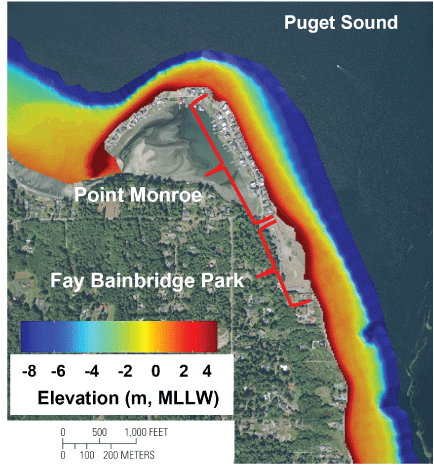
Interpolated bathymetry from acoustic survey and topographic data at Fay Bainbridge Park and Point Monroe, Bainbridge Island, Washington. Vertical datum is referenced to meters (m) above mean lower low water (MLLW).
Analyses and interpretation of acoustic survey data indicate that eelgrass is present along the entire shoreline of the Point Monroe and Fay Bainbridge study area (fig. 4). Both the total area of eelgrass and percentage eelgrass cover appears to be limited by water depth, with eelgrass observed mostly between 0.5 and -5 m MLLW, though a small quantity was observed in both shallower and deeper water. The most abundant and highest percentage cover of eelgrass were at water depths between -1 and -4 m MLLW. These findings are nearly identical to those determined in a similar Puget Sound eelgrass mapping survey (Stevens and others, 2008).
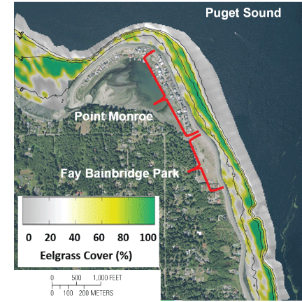
Percentage (%) cover of eelgrass at Fay Bainbridge Park and Point Monroe, Bainbridge Island, Washington. Interpolated data are from the raw fractional acoustic return data and bathymetric contour intervals are 2 meters (m).
Surf Smelt Spawning-Area Surveys
Surf smelt eggs were observed in greater quantity and within more segments along the southern Fay Bainbridge Park beach than were observed in samples collected from the more northerly Point Monroe. Eggs were present at 9 of the 14 (64.3 percent) segments that were sampled (table 1; fig.5), and eggs per sample were significantly higher at Fay Bainbridge Park than at Point Monroe (ANOVA; F1, 166 = 9.08, P =0.003; fig. 5). Every beach segment along Fay Bainbridge Park contained eggs, with eggs observed in 64 of the 84 (76.2 percent) samples. In total, 630 eggs were observed within the Fay Bainbridge Park sediments, comprising 540 live eggs and 90 dead eggs (14.3 percent mortality). The number of surf smelt eggs per segment ranged from 46 to 197, with a mean of 90 eggs per segment. Eggs were observed on 2 of the 7 segments along Point Monroe, but only on those segments located less than 100 m from Fay Bainbridge Park and that had shoreline armoring that was greater than 3.84 m above MLLW (fig. 5; table 1). Eggs were observed in 11 of the 84 (13.1 percent) Point Monroe samples. In total, 134 eggs were observed within the Point Monroe sediments, comprising 132 live eggs and 2 dead eggs (1.5 percent mortality). At Point Monroe, the number of surf smelt eggs per segment ranged from 0 to 116, with an average of 19 eggs per segment.
Table 1.
Surf smelt eggs observed and beach segment data collected at Fay Bainbridge Park and Point Monroe, Bainbridge Island, Washington.[mm, millimeter; m, meter; MLLW, mean lower low water; NA is not applicable]
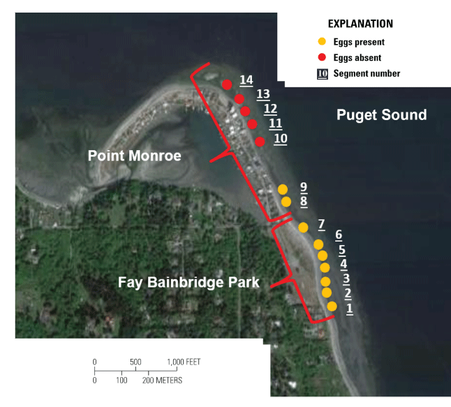
Surf smelt spawning survey segments denoting presence or absence of eggs at Fay Bainbridge Park and Point Monroe, Bainbridge Island, Washington. [m, meter]
Characteristics of bed sediment and habitat variables differed between Fay Bainbridge Park and Point Monroe (table 2). The mean sizes of sediment in samples collected from beach segments at the Fay Bainbridge Park were larger than the mean sizes of sediments collected from Point Monroe beach segments, and the differences were significant (ANOVA; F1, 166 = 24.43, P <0.001). The sorting of sediment grain sizes between the two sites were not significantly different, however (ANOVA; F1, 166 = 0.95, P =0.331), with the Point Monroe sediments being slightly less sorted than Fay Bainbridge Park sediments. Additionally, the percentage composition of sediment size classifications differed between the two sample sites. Fay Bainbridge Park sediments consisted primarily of gravel (80.30 percent), and the remainder was sand (19.69 percent). Most of the Point Monroe sediments also were gravels (58.73 percent), but the sand fraction was more than double (41.26 percent) that measured in the Fay Bainbridge Park sediments. The percentage occurrence of both gravel and sand were significantly different between sites (ANOVA; F1, 166 = 26.91, P <0.001 and F1, 166 = 26.92, P<0.001, respectively). Mud was virtually absent from both sample locations, comprising less than 1 percent of the total samples, and was not significantly different between sites (ANOVA; F1, 166 = 0.65, P =0.421). Shore slope and shoreline armoring also varied by sample location. The mean beach slope was 9.94 percent at Fay Bainbridge Park and a steeper 12.44 percent at Point Monroe and was significantly different between sites (ANOVA; F1, 166 = 222.70, P <0.001). In addition to differences in beach slope, no armoring was observed along the entirety of Fay Bainbridge Park, whereas at least a part of 6 of the 7 beach segments on Point Monroe were armored. The elevations at which samples were collected were significantly different between the two sites (ANOVA; F1, 166 = 21.26, P <0.001), with the mean elevation at Fay Bainbridge Park being higher on the beach than the Point Monroe mean elevation owing to armoring restricting the area of the upper beach on Point Monroe.
Characteristics of beach sediment and habitat variables where surf smelt eggs were present also showed some differences between Fay Bainbridge Park and Point Monroe (table 2). The mean sediment sizes in samples containing eggs from Fay Bainbridge Park beach segments were again larger than the mean sizes in sediment samples collected from the Point Monroe beach segments that contained eggs, and the differences were significant (ANOVA; F1, 73 = 6.69, P =0.012). The sorting of sediment grain sizes between the two sites were not significantly different, however (ANOVA; F1, 73 = 1.0, P =0.319), with the Fay Bainbridge Park sediments being slightly more sorted than Point Monroe sediments. The percentage composition of sediment size classifications of sample locations containing surf smelt eggs was similar to those observed in all sample locations. Fay Bainbridge Park sediments consisted primarily of gravel (78.82 percent), and the remainder was sand (21.28 percent). Most of the Point Monroe sediments were also gravels (59.72 percent), and the remainder sand. The percentage occurrence of both gravel and sand were significantly different between sites (ANOVA; F1, 73 = 7.02, P =0.01 and F1, 73 = 7.02, P =0.01, respectively). Again, mud was virtually absent in samples from both locations that contained surf smelt eggs and was not significantly different between sites (ANOVA; F1, 73 = 0.34, P =0.561). The mean beach slope for sample locations containing surf smelt eggs was 9.88 percent at Fay Bainbridge Park and a steeper 12.88 percent at Point Monroe and was significantly different between sites (ANOVA; F1, 73 = 44.66, P <0.001). Elevations of samples containing surf smelt eggs were similar at both Fay Bainbridge Park and Point Monroe and were not significantly different between sites (ANOVA; F1, 73 < 0.01, P =0.991).
Table 2.
Characteristics of beach sediment, slope, and elevation variables observed at all sample locations and at sample locations containing surf smelt eggs at Fay Bainbridge Park and Point Monroe, Bainbridge Island, Washington.[SD, standard deviation; m,meters; MLLW, mean lower low water; grain size units of phi (Φ) are calculated by a logarithmic transformation Φ = − log2 (d) where d represents the grain size diameter in mm]
Selection and Fit of Spawning Habitat Models
The influence of spatial autocorrelation on the presence of surf smelt spawning was non-significant (p = 0.57, r = -0.007), so additional adjustments for autocorrelation were not required. Simulation results showed that the best explanatory value occurred once covariates grain sorting and gravel were removed from the full model (as indicated by AIC; 174.74; table 3), with a deviance explained of 70.5 percent, an adjusted r2 of 0.35, and regression between the observed and fitted values that was indistinguishable from 1 (1.088). This model included variables such as elevation (p =0.06) and beach slope (p = 0.10), but the covariates that contributed the greatest impacts were grain size (p = 0.04), sand (p = 0.002), and armoring absence (p =0.02). Graphing of these variables show that as beach slope and grain size increase, the observations of spawning decrease (figs. 6A and 6B; respectively). Eggs were more abundant at higher elevations on the beach (fig. 6C), and there were fewer eggs observed as the proportion of sand increases (fig. 6D). The sign of the estimate (negative; -1.37) for armoring presence indicates that the presence of armoring negatively affects the presence of surf smelt eggs.
Table 3.
Model selection results showing the model, covariates, Akaike’s information criterion (AIC), the change in AIC from the AIC lowest model (ΔAIC; model 3), and the percentage deviance explained.[**, p-value less than 0.01; *, p-value less than 0.05]
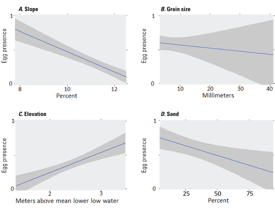
The influence of beach habitat covariates on surf smelt egg presence at Fay Bainbridge Park and Point Monroe, Washington. The y-axis denotes either the absence of eggs (0) or the presence of eggs (1). Continuous variables are percentage slope (A), grain size (in millimeters; B), elevation (in meters above mean lower low water; (C), and percentage sand (D). The solid line is the regression prediction, and the shaded areas indicate the 95 percent standard error of the prediction.
Sea Level Rise Modeling
Under all SLR scenarios, the SLAMM simulations predicted changes in habitat types from 2010 to 2100 within our study area (table 4). As expected, simulation of the most conservative scenario (A1B Mean) predicted the least change, followed by the 1-m scenario, and the 2-m scenario predicted the greatest amount of conversion of beach and upland habitat to open water. For all scenarios, the simulations predicted that swamps, tidal flats, and vegetated tidal flats were vulnerable to loss, but the initial area occupied by these habitat types was small. Under the A1B-mean scenario, both developed and undeveloped dry land lost 10 percent of their extent and were converted to transitional saltwater marsh and regularly flooded marsh habitat categories (fig. 7). The predictions of the 1-m SLR scenario were similar to the A1B-mean scenario except for estuarine beaches, which were reduced 6 percent in size (fig. 7). As expected, the greatest amount of habitat change occurred using the 2-m SLR scenario. The area of undeveloped dry land in the 2-m SLR scenario remained similar to the other scenarios, but as much as 53 percent of the developed dry land could be subjected to inundation and converted to transitional salt marsh (fig. 7). Additionally, this scenario predicted the conversion of 13 percent of the estuarine beach to open water. The loss of developed dry land and estuarine beach is predicted to occur primarily at Point Monroe.
Table 4.
Projections of area of habitat categories (in hectares) and percentage change (in parentheses) using the A1B Mean (0.4 meters), 1-meter, and 2-meter sea-level rise scenarios for 2100 at Fay Bainbridge Park and Point Monroe, Bainbridge Island, Washington, using the Sea Level Affecting Marshes Model (SLAMM).[SLR, sea level rise; NA is not applicable]
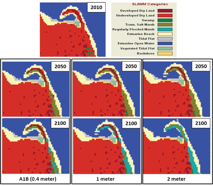
Simulated projections of habitat change at Fay Bainbridge Park and Point Monroe, Washington. Simulations project the years 2050 and 2100, under the A1B Mean (0.4 meter), 1-meter, and 2-meter sea-level rise scenarios with the Sea Level Affecting Marshes Model (SLAMM).
When SLAMM sea level predictions were overlaid on existing eelgrass habitat, the potential available habitat for eelgrass increased with increasing SLR (table 5). The model predicts that eelgrass habitat will be lost at the lower depth margins owing to light attenuation at increased water depth, but an increase in the inundation of the current intertidal beach adjacent to the existing eelgrass beds will allow for landward expansion to compensate for that loss. The least amount of eelgrass habitat gain occurred under the A1B Mean scenario (10.2 percent), followed by 22.1 percent increase under the 1-m SLR scenario, while the 2-m SLR scenario had the greatest increase in potential eelgrass habitat (37.6 percent).
Surf smelt use habitat falls within the SLAMM estuarine beach habitat category for deposition of their eggs during spawning. Under all three SLR scenarios, the area of potential surf smelt spawning habitat was reduced (table 5). The smallest amount of estuarine beach habitat loss occurred under the A1B-mean scenario (1.8 percent), followed by a 6.1 percent loss under the 1-m SLR scenario, and the 2-m SLR scenario had the greatest loss of potential surf smelt spawning habitat (12.8 percent). The beaches around Point Monroe experienced the greatest loss of estuarine beach habitat (fig. 7), primarily because shoreline armoring prevented beach formation from moving landward, as was possible along Fay Bainbridge Park beaches where armoring was absent.
Table 5.
Projections of area of surf smelt spawning habitat and eelgrass habitat changes (in hectares) and percentage (in parentheses) using the A1B Mean (0.4 meters), 1-meter, and 2-meter sea-level rise scenarios for 2100 at Fay Bainbridge Park and Point Monroe, Bainbridge Island, Washington, using the Sea Level Affecting Marshes Model (SLAMM).Discussion—Current Status and Effects of Sea Level Rise on Changes in Nearshore Habitat
Results of our SLR modeling indicate that several changes in beach and adjacent upland habitats are likely to occur with increasing water-level elevations in the Puget Sound. SLAMM simulation results depict that under all SLR scenarios, swamps, tidal flats, vegetated tidal flats, and estuarine beach are vulnerable to conversion to open water. Most striking though, under the most conservative SLR scenario, both developed and undeveloped dry land is predicted to experience a 10-percent decrease of their current area by 2100. In the simulation of the most extreme SLR scenario, the reduction of developed dry land along Point Monroe could be more than 50 percent of the current area, assuming no further development or shoreline alterations occur.
Our study area lies near the terminus of a drift cell (Skiff Point to Point Monroe Drift Cell; MacLennan and others, 2010), where sandy spits and other accretionary shore forms tend to occur. Within the study area, we observed the customary decrease in sediment size near the end of the drift cell caused by sediment transport. At Point Monroe, however, there was an increase in beach slope and decrease in beach width, which are not generally associated with natural processes of accretionary shore forms. Beach sediments along the low tide terrace were generally similar at both sites, but differences were observed at the upper beach. At Fay Bainbridge Park, the upper beach consisted of sediments of greater mean size than the sediments at Point Monroe. Additionally, the beaches along Point Monroe were steeper than those along Fay Bainbridge Park. These results suggest that wave energy at the armored upper beach at the Point Monroe site is affecting beach sediment size composition and beach morphology that is not observed along the unarmored upper beach of Fay Bainbridge Park. With the predicted SLR, it is likely that these differences would become exacerbated.
Both contiguous and patchy eelgrass beds were observed along most of the study area, with the most contiguous beds along the northeast facing aspect. These beds were observed primarily at water depths from -1 to -4 m MLLW. Contrary to our initial hypothesis, the projected available eelgrass habitat increased with increasing sea level in the survey area. However, it is unknown which specific physical or mechanical responses (such as, accretion, scour, or slope) a specific beach will undergo with changes in sea level, or with SLR-induced effects such as increasing storm surge and wave energy. At these shallow elevations, this potential eelgrass habitat is likely to be sensitive to sediment re-suspension and sunlight attenuation that could restrict eelgrass establishment and growth (Orth and others, 2006).
Surf smelt eggs were observed on the beaches within our study area, primarily along the undeveloped beaches of Fay Bainbridge Park. Surf smelt eggs were observed only on Point Monroe beach segments that were immediately adjacent to Fay Bainbridge Park segments, and shoreline armoring at those sites were greater than 3.84 m above MLLW in elevation. No eggs were observed where shoreline armoring was below that elevation. These results indicate that shoreline armoring below a critical elevation could be a physical barrier to use by surf smelt at this location, and additional study is warranted to confirm this observation. With increasing sea level, and the probable reduction in the availability of estuarine beach habitat that is used by surf smelt, the potential spawning habitat at Point Monroe could progressively deteriorate.
Because predictions of the magnitude of future SLR remain indeterminate, we simulated a range of SLR estimates in our study. Habitat modeling addresses the likely land-use changes and local habitat topography to the nearshore environment with elevated sea level but does not account for probable alterations to beach sediments, beach profile, or habitat suitability. Compounding the effects of SLR on the nearshore environment, shoreline armoring can alter the morphologic and sediment-transport processes associated with local beach sediments (Kraus and McDougal, 1996), possibly reducing habitat suitability for both eelgrass and surf smelt. Our results demonstrate that the differences in upper beach sediments and beach gradient on the beaches of Point Monroe are likely indicative of shoreline armoring impacts such as sediment scour and wave reflection (Griggs, 2005; Miles and others, 2001; Ruggiero, 2010). This is expected, as shoreline armoring creates a distinct demarcation between the land and the sea (Dugan and others, 2008) creating an abrupt transition, or ecotone, between marine and terrestrial communities (Heerhartz and others, 2014). The unarmored beaches along Fay Bainbridge Park showed greater plasticity for habitat succession, as the estuarine beach was not prohibited from migrating inland with increasing sea level. Thus, it is likely that this plasticity will reduce the risk of the substantial loss of eelgrass and surf smelt spawning habitat caused by SLR at this location. Although this study was made along a single stretch of beach, these results are likely applicable to other beaches within Puget Sound to estimate potential nearshore habitat alterations caused by SLR.
Acknowledgments
We thank the staff of Fay Bainbridge Park and the residents of Point Monroe for their permission to access beaches for data collection. Thanks to Patty Glick (National Wildlife Federation) and Jonathan Clough (Warren Pinnacle Consulting, Inc.) for providing the Puget Sound SLAMM data and technical assistance. We thank all U.S. Geological Survey staff who assisted in this study for their perseverance, dedication, and understanding, and especially thank Andrew Stevens for sharing his hydroacoustic survey expertise. Thanks to the U.S. Geological Survey, Northwest Area Regional Executive, FY2010 Flex Funds program for financial support, and the Washington Department of Fish and Wildlife for the required collection permit (Permit # 10-206).
References Cited
Church, J.A., Clark, P.U., Cazenave, A., Gregory, J.M., Jevrejeva, S., Levermann, A., Merrifield, M.A., Milne, G.A., Nerem, R.S., Nunn, P.D., Payne, A.J., Pfeffer, W.T., Stammer, D., and Unnikrishnan, A.S., 2013, Sea level change, in Stocker, T.F., Qin, D., Plattner, G.-K., Tignor, M., Allen, S.K., Boschung, J., Nauels, A., Xia, Y., Bex, V., and Midgley, P.M., eds., Climate change 2013—The physical science basis—Contribution of working group I to the fifth assessment report of the Intergovernmental Panel on Climate Change: Cambridge, United Kingdom, Cambridge University Press, p. 1137–1216.
Clough, J.S., and Larson, E.C., 2010, Application of the Sea Level Affecting Marshes Model (SLAMM 6) to Willapa NWR: Arlington, Virginia, U. S. Fish and Wildlife Service, National Wildlife Refuge Service, prepared by Warren Pinnacle Consulting, Inc., 72 p., accessed July 1, 2020, at http://warrenpinnacle.com/prof/SLAMM/USFWS/SLAMM_Willapa_NWR.pdf.
Clough, J.S., Park, R.A., and Fuller, R., 2010, SLAMM 6 beta, technical documentation, (release 6.0 beta): Warren, Vermont, Warren Pinnacle Consulting, Inc., 51 p., accessed July 1, 2020, at http://warrenpinnacle.com/prof/SLAMM6/SLAMM6_Technical_Documentation.pdf.
Donoghue, J.F., Elsner, J.B., Hu, B.X., Kish, S.A., Niedoroda, A.W., Wang, Y., and Ye, M., 2013, Effects of near-term sea-level rise on coastal infrastructure. SERDP Project RC-1700: Alexandria, Virginia, Department of Defense Strategic Environmental Research and Development Program, 186 p., accessed July 1, 2020, at https://www.serdp-estcp.org/Program-Areas/Resource-Conservation-and-Resiliency/Infrastructure-Resiliency/Vulnerability-and-Impact-Assessment/RC-1700.
Glick, P., Clough, J., and Nunley, B., 2007, Sea-level rise and coastal habitats in the Pacific Northwest—An analysis for Puget Sound, Southwestern Washington, and Northwestern Oregon: Seattle, Washington, National Wildlife Federation, 94 p., accessed July 1, 2020, at https://www.nwf.org/~/media/PDFs/Water/200707_PacificNWSeaLevelRise_Report.ashx.
Intergovernmental Panel on Climate Change (IPCC), 2007, Climatic Change 2007—Synthesis report: Geneva Switzerland, 104 p., accessed July 1, 2020, at https://www.ipcc.ch/report/ar4/syr/.
Intergovernmental Panel on Climate Change (IPCC), 2019, IPCC Special Report on the Ocean and Cryosphere in a Changing climate: Geneva, Switzerland, 765 p., accessed July 1, 2020, at https://www.ipcc.ch/site/assets/uploads/sites/3/2019/12/SROCC_FullReport_FINAL.pdf.
Johnson, S.W., Thedinga, J.F., Neff, A.D., Heintz, R.A., Lindeberg, M.R., Harris, P.M., and Rice, S.D., 2008, Seasonal distribution, habitat use, and energy density of forage fish in the nearshore ecosystem of Prince William Sound, Alaska: Anchorage, Alaska, North Pacific Research Board Final Report 642, 94 p., accessed July 1, 2020, at http://www.pws-osri.org/business/0702advboard/4.2%20Johnson%20Progress%20Report%20Jan%2015%202007.pdf.
Keuler, R.F., 1988, Map showing coastal erosion, sediment supply, and longshore transport in the Port Townsend 30- by 60- minute quadrangle, Puget Sound Region, Washington: U.S. Geological Survey Miscellaneous Investigations Map 1198-E, accessed November 27, 2020, at https://pubs.er.usgs.gov/publication/i1198E.
Krueger, K.L., Pierce, K.B., Quinn, T., and Penttila, D.E., 2010, Anticipated effects of sea level rise in Puget Sound on two beach-spawning fishes: Olympia, Washington, Washington Department of Fish and Wildlife, Habitat Program, 8 p., accessed July 1, 2020, at https://wdfw.wa.gov/sites/default/files/publications/01210/wdfw01210.pdf.
Lentz, E.E., Stippa, S.R., Thieler, E.R., Plant, N.G., Gesch, D.B., and Horton, R.M., 2015, Evaluating coastal landscape response to sea-level rise in the northeastern United States—Approach and methods: U.S. Geological Survey Open-File Report 2014–1252, 26 p., accessed July 1, 2020, at https://doi.org/10.3133/ofr20141252.
MacLennan, A., Johannessen, J., and Williams, S., 2010, Bainbridge Island current and historic coastal geomorphic/feeder bluff mapping: Bellingham, Washington, Coastal Geologic Services, Inc., 53 p., accessed July 2, 2021, at https://www.bainbridgewa.gov/DocumentCenter/View/1765/Drift-Cell-Report-PDF.
McNamara, D., and Keeler, A. A., 2013, Coupled physical and economic model of the response of coastal real estate to climate risk: Nature Climate Change, v. 3, p. 559–562, accessed July 1, 2020, at https://doi.org/10.1038/nclimate1826.
Meehl, G.A., Stocker, T.F., Collins, W.D., Friedlingstein, P., Gaye, A.T., Gregory, J.M., Kitoh, A., Knutti, R., Murphy, J.M., Noda, A., Raper, S.C.B., Watterson, I.G., Weaver, A.J., and Zhao, Z.-C., 2007, Global climate projections, in Solomon, S., Qin, D., Manning, M., Chen, Z., Marquis, M., Averyt, K.B., Tignor, M., and Miller, H.L., eds., Climate Change 2007—The physical science basis. Contribution of Working Group I to the Fourth Assessment Report of the Intergovernmental Panel on Climate Change: New York, New York, Cambridge University Press, p. 747–845.
Moulton, L.L., and Penttila, D., 2001, Field manual for sampling forage fish spawn in intertidal shore regions: Olympia, Washington, San Juan County Forage Fish Assessment Project, 27 p., accessed July 1, 2020, at https://wdfw.wa.gov/publications/01209.
Mumford, T.F., 2007, Kelp and eelgrass in Puget Sound—Puget Sound Nearshore Partnership Report No. 2007-05: Seattle, Washington, U.S. Army Corp of Engineers, 34 p., accessed July 1, 2020, at https://wdfw.wa.gov/publications/02195.
National Oceanic and Atmospheric Administration, 2020, Station 9447130 Seattle, Washington: Center for Operational Oceanographic Products and Services, accessed July 1, 2020, at https://tidesandcurrents.noaa.gov/stationhome.html?id=9447130.
National Resource Council, 2012, Sea-Level Rise for the Coasts of California, Oregon, and Washington—Past, Present, and Future: Washington, D.C., The National Academies Press, 216 p., accessed July 1, 2020, at https://nap.nationalacademies.org/catalog/13389/sea-level-rise-for-the-coasts-of-california-oregon-and-washington.
Penttila, D., 2007, Marine forage fishes in Puget Sound. Puget Sound Nearshore Partnership Report No. 2007-03: Seattle, Washington, U.S. Army Corps of Engineers, 30 p., accessed July 1, 2020, at https://wdfw.wa.gov/publications/02193.
Plant, N.G., Flocks, J.G., Stockdon, H.F., Long, J.W., Guy, K.K., Thompson, D., Cormier, J., Smith, C.G., Miselis, J.L., and Dalyander, P.S., 2014, Predictions of barrier island berm evolution in a time‐varying storm climatology: Journal of Geophysical Research—Earth Surface, v. 119, no. 2, p. 300–316.
Puget Sound Partnership (PSP), 2008, Puget Sound action agenda—Protecting and restoring the Puget Sound ecosystem by 2020: Olympia, Washington, Puget Sound Partnership, 207 p., accessed July 1, 2020, at https://pspwa.app.box.com/s/kuhc0eyk1rkxcd0mt53q79c0d8jt09wn/file/72089838717.
R Core Team, 2014, R—A language and environment for statistical computing, version 4.0.3: Vienna, R Foundation for Statistical Computing software release, accessed July 1, 2020, at http://www.R-project.org/.
Raymond, C., Conway-Cranos, L., Morgan, H., Faghin, N., Spilsbury Pucci, D., Krienitz, J., Miller,I., Grossman, E., and Mauger, G., 2018, Sea level rise considerations for nearshore restoration projects in Puget Sound: Seattle, Washington, Washington Coastal Resilience Project, 41 p., accessed July 1, 2020, at https://cig.uw.edu/publications/sea-level-rise-considerations-for-nearshore-restoration-projects-in-puget-sound/.
Ruggiero, P., 2010, Impacts of shoreline armoring on sediment dynamics, in Shipman, H., Dethier, M.N., Gelfenbaum, G., Fresh, K.L., and Dinicola, R.S., eds., Puget Sound shorelines and the impacts of armoring—Proceedings of a state of the science workshop, May 2009: U.S. Geological Survey Scientific Investigations Report 2010–5254, p. 179–186, accessed July 1, 2020, at https://pubs.usgs.gov/sir/2010/5254/.
Sabol, B.M., Burczynski, J., and Hoffman, J., 2002, Advanced digital processing echo sounder signals for characterization of very dense submersed aquatic vegetation: Vicksburg, Mississippi, U.S. Army Corps of Engineer Research and Development Center, ERDC/EL TR-02-30, 25 p., accessed July 1, 2020, at https://erdc-library.erdc.dren.mil/jspui/bitstream/11681/7025/1/ERDC-EL%20TR-02-30.pdf.
Sallenger, A.H., Jr., Krabill, W.B., Swift, R.N., Brock, J., List, J., Hansen, M., Holman, R.A., Manizade, S., Sontag, J., Meredith, A., Morgan, K., Yunkel, J.K., Frederick, E.B., and Stockdon, H., 2003, Evaluation of airborne topographic Lidar for quantifying beach changes: Journal of Coastal Research, v. 19, no. 1, p. 125–133.
Stevens, A.W., Lacy, J.R., Finlayson, D.P., and Gelfenbaum, G., 2008, Evaluation of a single-beam sonar system to map seagrass at two sites in northern Puget Sound, Washington: U.S. Geological Survey Scientific Investigations Report 2008–5009, 45 p., accessed July 1, 2020, at https://pubs.usgs.gov/sir/2008/5009/sir2008-5009.pdf.
Tomka, R.G., Smith, C.D., and Liedtke, T.L., 2020, Data collected in 2010 to evaluate habitat availability for surf smelt and eelgrass in response to sea level rise on Bainbridge Island, Puget Sound, Washington State, USA: U.S. Geological Survey data release, https://doi.org/10.5066/P9HGJ3ZHf.
Williams, G.D., and Thom, R.M., 2001, Marine and estuarine shoreline modification issues: Battelle Marine Sciences Laboratory and Pacific Northwest National Laboratory, Sequim, Washington, 140 p., accessed July 1, 2020, at https://wdfw.wa.gov/sites/default/files/publications/00054/wdfw00054.pdf.
Williams, G.D., Thom, R.M., and Evans, N.R., 2004, Bainbridge Island nearshore habitat characterization and assessment, management strategy prioritization, and monitoring recommendations—PNWD-3391: Bainbridge Island, Washington, City of Bainbridge Island, prepared by Battelle Marine Sciences Laboratory, Sequim, Washington, 250 p., accessed July 1, 2020, at http://www.ci.bainbridge-isl.wa.us/DocumentCenter/View/2555.
Conversion Factors
International System of Units to U.S. customary units
Temperature in degrees Celsius (°C) may be converted to degrees Fahrenheit (°F) as:
°F = (1.8 × °C) + 32.
Datums
Vertical coordinate information is referenced to the National Geodetic Vertical Datum of 1929 (NGVD 29).
Elevation, as used in this report, refers to distance above the vertical datum.
Supplemental Information
Concentrations of chemical constituents in water are in milligrams per liter (mg/L).
Publishing support provided by the U.S. Geological Survey
Science Publishing Network, Tacoma Publishing Service Center
For more information concerning the research in this report, contact the
Director, Western Fisheries Research Center
U.S. Geological Survey
6505 NE 65th Street
Seattle, Washington 98115-5016
Suggested Citation
Smith, C.D., and Liedtke, T.L., 2022, Potential effects of sea level rise on nearshore habitat availability for surf smelt (Hypomesus pretiosus) and eelgrass (Zostera marina), Puget Sound, Washington: U.S. Geological Survey Open-File Report 2022–1054, 17 p., https://doi.org/10.3133/ofr20221054.
ISSN: 2331-1258 (online)
Study Area
| Publication type | Report |
|---|---|
| Publication Subtype | USGS Numbered Series |
| Title | Potential effects of sea level rise on nearshore habitat availability for surf smelt (Hypomesus pretiosus) and eelgrass (Zostera marina), Puget Sound, Washington |
| Series title | Open-File Report |
| Series number | 2022-1054 |
| DOI | 10.3133/ofr20221054 |
| Year Published | 2022 |
| Language | English |
| Publisher | U.S. Geological Survey |
| Publisher location | Reston, VA |
| Contributing office(s) | Western Fisheries Research Center |
| Description | Report: v, 17 p.; Data Release |
| Country | United States |
| State | Washington |
| Other Geospatial | Puget Sound |
| Online Only (Y/N) | Y |
| Google Analytic Metrics | Metrics page |