

Extending the Stream Salmonid Simulator to Accommodate the Life History of Coho Salmon (Oncorhynchus kisutch) in the Klamath River Basin, Northern California
Links
- Document: Report (10.8 MB pdf) , HTML , XML
- Download citation as: RIS | Dublin Core
Acknowledgments
This work was funded by Interagency Grant number R16PG00053 from the Bureau of Reclamation to the U.S. Geological Survey. We are grateful to staff of multiple State, Federal, and Tribal agencies that have collected the field data on which our modeling efforts are based. Data are not currently available from the funding organization. Contact the Bureau of Reclamation for further information.
Abstract
In this report, we apply the stream salmonid simulator (S3) to coho salmon (Oncorhynchus kisutch) in the Klamath River Basin by extending the original model to account for life history and disease dynamics specific to coho salmon. This version of S3 includes tracking of three separate life-history strategies representing the different time periods and ages at which fish leave natal tributaries such as the Scott and Shasta Rivers (age-0 spring, age-0 fall, or age-1 smolt). Once fish leave their natal tributaries and enter the Klamath River, the deterministic life-stage-structured population model simulates daily growth, movement, and survival. We extend the model to include non-natal tributary dynamics, where spring age-0 fish entry to non-natal tributaries is simulated based on environmental conditions in the main-stem Klamath River. Fish that use non-natal tributaries then reenter the Klamath River during the winter or spring as smolts and actively migrate downstream. We also consider the life history strategy where fish rear in natal tributaries and enter the Klamath River as age-1 smolts. In addition to simulating different life history pathways that coho salmon may take, we model disease dynamics, incorporating new information on Ceratonova shasta related infection and mortality. We incorporate competitive interactions between juvenile coho and Chinook salmon (Oncorhynchus tshawytscha) by simulating density-dependent movement dynamics in response to Chinook salmon abundance.
Model simulations suggest that total abundance and survival to the ocean differed between life-history strategies. In general, spring age-0 fish that leave their natal tributaries in their first spring had lower survival compared with fish that remained in natal tributaries and out-migrated later. Spring age-0 fish also had higher disease related mortality, owing to their residence in the main-stem Klamath River overlapping with periods of elevated C. shasta spore concentrations. Age-0 fish leaving their natal tributaries in the fall had near-zero disease related mortality. Most non-natal tributary use occurred at upstream tributary locations and was variable between the brood years depending on passage timing and environmental conditions. The inclusion of Chinook salmon in simulations resulted in decreased abundance and survival of Coho salmon reaching the ocean. In addition, we developed an R package to facilitate use of and continued development of S3 as a tool to guide management of juvenile salmonid populations.
Introduction
Background
This report details the application of the stream salmonid simulator (S3) to coho salmon (Oncorhynchus kisutch) in the Klamath River, northern California (fig.1). The S3 is a deterministic life-stage-structured population model that simulates daily growth, movement, and survival of juvenile salmonids. Here, we document the application of S3 to coho salmon, focusing on several themes relevant to management, including disease dynamics and variation in life history strategies. We build from previous applications of the S3 model to Chinook salmon (Oncorhynchus tshawytscha) in the Klamath River Basin (Perry, Jones, and others, 2018; Perry and others, 2019), expanding the domain to which the S3 model has been applied.
The S3 model was developed to aid fisheries and water managers in understanding the impacts of alternative management actions on anadromous fish populations (Plumb and others, 2019). The model links the effects of river flow to habitat availability and capacity, which drives density-dependent population dynamics in a series of linked habitat units. The environmental template of each habitat unit is defined by a time series of daily discharges, water temperatures, and usable habitat areas or carrying capacities. Survival, growth, and movement processes are simulated for juvenile salmonids in each of these habitat units.
Coho salmon within the Klamath River Basin are classified in the southern Oregon and northern California Evolutionarily Significant Unit and recognized as threatened under the Endangered Species Act (Federal Register, 1997). The decline of coho salmon in the Klamath River Basin is due to a myriad of factors, including construction of main stem dams and agricultural demand for water. The main-stem Klamath River has extensive hydropower development, including dams constructed during the first half of the 20th century that not only limit fish passage within the basin, but alter river discharge and water temperature. Downstream from the lowermost dam, Iron Gate Dam, decreased summer discharge, elevated water temperatures, and decreased habitat availability and water quality are of particular concern for coho and Chinook salmon.
Coho salmon in the Klamath River Basin are affected by alterations to flow and temperature regimes. Increased water temperatures have been cited as a leading factor limiting the recovery of salmonids in the basin (Bartholow, 2005). Salmonids, including coho salmon, are often observed using thermal refuges provided by cold water tributaries in the Klamath River (Sutton and others, 2007). This behavioral strategy may help to limit the increased metabolic costs associated with elevated temperatures in the main-stem Klamath River. Lower flows can also directly impact coho salmon by limiting the amount of rearing habitat and slowing rates of downstream migration, potentially decreasing survival due to increased exposure to predation and disease (Čada and others, 1997). Alterations to flow regimes not only occur in the main-stem Klamath River but in the major tributaries as well (National Research Council, 2004).
The Scott and Shasta Rivers are two of the primary sources of naturally produced coho salmon in the upper anadromous Klamath River (Chesney and Knechtle, 2015; Knechtle and Chesney, 2016). Flows in these tributaries are impacted by surface-water diversions and groundwater pumping for agriculture (National Research Council, 2004). Loss of riparian buffer, water diversions, and decreased cold water spring inputs have contributed to increases in water temperatures (Nichols and others, 2014). Altered hydrology and elevated temperatures are two primary factors threatening coho salmon produced in the Scott and Shasta Rivers.
Coho salmon can have a complex life history with migratory events often occurring between large main-stem rivers and non-natal tributaries (Lestelle, 2007). In the upper anadromous Klamath River, natural production occurs in both large rivers (for example, Scott and Shasta Rivers) and smaller perennial tributaries. Much has been learned about the life history dynamics of naturally produced coho salmon from the Scott and Shasta Rivers owing to annual juvenile trapping efforts and tagging studies using passive integrated transponder (PIT) tags (Manhard and others, 2018a). Juveniles emigrate from natal tributaries at various life stages, either as age-0 fry and parr in the spring and fall, or as age-1 smolts the following spring. Age-0 migrants that enter the main-stem Klamath River in spring typically seek refuge from rising summer water temperatures in the main stem by migrating into non-natal tributaries (Sutton and others, 2007; Sutton and Soto, 2012). Juvenile coho salmon that use non-natal tributaries will migrate back into the main-stem Klamath River when environmental conditions are more favorable, typically during the following winter or spring periods (Manhard and others, 2018a). After reentering the main-stem Klamath River from non-natal tributaries, these juveniles actively migrate downstream as age-1 smolts. Less is known about the fall age-0 migrants that leave the Scott and Shasta Rivers because screw traps on natal tributaries are not operated during this period. Juvenile coho salmon are often observed entering non-natal tributaries during the winter, and these fish may represent some fraction of fall age-0 migrants; however, the source of these fish is uncertain (Witmore, 2014; Manhard and others, 2018a). Fish that overwinter in the Scott and Shasta Rivers leave during the following spring and actively migrate downstream in the main-stem Klamath River as age-1 smolts.
Naturally produced juvenile coho salmon co-occur with both naturally and hatchery produced Chinook salmon in the Klamath River Basin. Juvenile Chinook salmon occur in high densities as a result of hatchery programs that can release up to 5 million smolts annually, and extant populations having not decreased to abundances as low as coho salmon in the area. Interspecific competition can occur in salmonids, where juveniles are territorial and compete for space or shared resources, which may ultimately result in decreased size or survival (Hearn, 1987; Fausch, 1988). Both coho and Chinook salmon occupy similar habitats when rearing in streams and show similar levels of aggression (Lister and Genoe, 1970; Stein and others, 1972). High densities of juvenile coho and Chinook salmon using similar habitat would suggest that some level of competition may occur in the Klamath River.
Modeling Disease Impacts on Juvenile Coho Salmon
Disease can be a major source of mortality in juvenile Pacific salmon (Oncorhychus spp.), including coho salmon in the Klamath River (Fujiwara and others, 2011; Ray and others, 2014). Mitigating the effects of the myxozoan parasite Ceratonova shasta on coho and Chinook salmon is a particular management concern. The parasite has a complicated life cycle with two distinct spore stages and two obligate hosts, a salmonid and a freshwater annelid (Manayunkia occidentalis). Myxospores released from infected salmonid hosts infect the annelid hosts, and actinospores released from infected annelid hosts infect salmonids. C. shasta infects multiple salmonid species, and genetically distinct strains (genotypes I, II, and 0) vary in specificity and virulence in their respective fish hosts. Although all genotypes appear to be able to infect most salmonid hosts, they differ in specificity and virulence. Genotype 0 is most commonly detected in rainbow trout (Oncorhynchus mykiss) but is not typically associated with mortality (Atkinson and Bartholomew, 2010). Genotype I also is a specialist that infects and causes mortality in Chinook salmon. Genotype II is a generalist and is associated with mortality in coho salmon, sockeye salmon (Oncorhynchus nerka), and chum salmon (Oncorhynchus keta) (Hallett and others, 2012; Hurst and Bartholomew, 2012). Although the parasite infects and causes disease in adult and juvenile salmonids in the Klamath River, disease is associated with mortality primarily in juvenile salmonids. C. shasta induced mortality ranging from 0 to greater than 90 percent of age-0 fish is observed in coho and Chinook salmon in sentinel exposure trials (Hallett and others, 2012; Ray and others, 2012), and evidence indicates that C. shasta can influence population dynamics (Fujiwara and others, 2011).
Management actions have recently been implemented at Klamath River dams to mitigate the effects of C. shasta on salmon populations. These management actions consist of flushing flows to scour the annelid host populations that release actinospores and dilution flows intended to reduce the concentration of actinospores (Alexander and others, 2016; Shea and others, 2016). Although modeling studies have simulated a decrease in population-level mortality associated with these management actions (Plumb and others, 2019; Som and others, 2019), the degree to which these management actions are having population-level impacts is uncertain. Thus, improving our understanding of the population-level response to management actions and the impact of future environmental change requires development of analytical tools tailored for coho salmon in the Klamath River Basin. The S3 model detailed in this report is one such tool that integrates our understanding of coho salmon life history, disease ecology, and variation in biological and environmental conditions to assess the population level responses.
Purpose and Scope
Given the threats to coho salmon in the Klamath River Basin and the importance of assessing alternative management actions, we developed a version of the S3 model specific to coho salmon. This model characterizes the dynamics of juvenile coho salmon in freshwater in relation to environmental and biological conditions. Specifically, this version of the S3 model accommodates alternative life-history strategies of naturally produced coho salmon in the Klamath River Basin that includes overwintering and non-natal tributary rearing. We then use the model to assess disease dynamics and quantify the population-level impacts of C. shasta over the historical period during which spore concentrations have been measured. We also assess the impacts of juvenile Chinook salmon on coho salmon using a density-dependent movement submodel within S3.
Methods
Disease Modeling
The temporal dynamics of mortality from C. shasta in salmonids typically have three characteristic traits, described by Ray and others (2014) as delayed onset of mortality following initial exposure, a period of rapid mortality, and a plateau where no additional mortality occurs. To parameterize a coho salmon-specific disease model in S3, we used the same analytical approach described in Perry and others (2019), where we fit a survival cure model to sentinel trial data. We extend the work of Ray and others (2014) by analyzing a more recent set of sentinel experiments that incorporated a range of exposure durations into the study design. Because coho salmon mortality is induced by the genotype II of C. shasta (Atkinson and Bartholomew, 2010), all analysis and simulations are based on measurements of genotype II spores. Here, we briefly describe the sentinel experiments that were used to develop the survival cure model. The sentinel trials were designed to quantify how C. shasta induced mortality is influenced by exposure duration, spore concentration during exposure, water temperature during exposure, and water temperature post exposure. We used data from n = 24 sentinel trials conducted in 2014 and 2015; each trial was conducted by:
-
Exposing 23–32 juvenile coho salmon held in cages in the infectious zone for 1–7 days;
-
Measuring daily C. shasta spore concentration and water temperature during the exposure period (water samples were collected every 2 hours and pooled for the day, while water temperature was collected hourly and averaged for the day);
-
Transporting fish to the J.L. Fryer Aquatic Animal Health Laboratory at Oregon State University where fish were held at water temperatures of 13 °C, 15 °C, or 18 °C; and
-
Recording the time to death of each fish for up to 90 days, at which point the number of survivors was recorded.
We used a survival cure model, similar to the approach used by (Ray and others, 2014) to model survival of fish exposed to C. shasta in experimental trials (table 1). The survival cure model is composed of two components: (1) a “cure” probability, which is the proportion of the population expected to survive the disease, and (2) a time-to-death function for individuals expected to die from disease:
whereS(t)
is the overall probability of surviving t days after infection,
π
is the proportion of fish that become infected and eventually die from ceratomyxosis, and
S(t|death)
is the proportion of fish that survive to time t of those expected to die from C. shasta.
Table 1.
Summary of sentinel trials used to fit the survival cure model used in stream salmonid simulator, 2014–15.[Exposure duration: E, d, exposure duration, in days. Mean exposure temperature: TE, °C, mean water temperature during exposure period, in degrees Celsius. Holding temperature: TH, °C, water temperature during holding period, in degrees Celsius. Mean spore concentration: C, spores/L, total genotype II Ceratonova shasta spore concentration, in spores per liter]
The data required to fit the model is the vector xi = (ti, ci), where ti is either the recorded time of death of the ith individual or the censoring time (that is, the time when the trial ended if the ith fish remained alive for the duration of the trial), and ci is the censoring indicator (ci = 0 if ti = time of death, ci = 1 if the ti = trial duration). The cure model allows both the probability of infection and eventual death, π, and the time-to-death, S(t|death), to be modeled separately as functions of covariates.
For π, the covariates and model structure were determined by a previous analysis of this dataset by Som and others (2019). They found that the best-fit model structure on the total mortality in each sentinel trial included genotype II spore concentration, water temperature during exposure period, water temperature during the post-exposure holding period (holding temperature), exposure duration, and an interaction between exposure temperature and holding temperature. This model structure for π was held fixed across all models evaluating time to death “S(t|death),” but the coefficients associated with the covariates for π were estimated jointly with the covariates for S(t|death).
Given the model structure for π, we used a three-step model selection approach, using Akaike’s information criterion (AIC) to arbitrate between models for S(t|death). First, we fit a model set with alternative distributions for S(t|death) and compared these using AIC. We considered five distributions, including the Weibull, log-normal, gamma, log-logistic, and generalized F distributions. This set of models was fit using all main effects and all possible two-way interactions. Second, we used the most highly supported distribution and fit four models evaluating support for either spore concentration or the natural logarithm of spore concentration. With spore concentration and the logarithm of spore concentration, we fit two models each containing either full covariates with interactions or main effects only. We then chose the model with the lowest AIC and proceeded with our last model selection step. We evaluated interaction terms by removing each term one at a time and keeping only interaction terms that reduced AIC by more than 10 units. Within this set of models, we selected the model with the lowest AIC to evaluate and incorporate into S3.
In addition to providing the parameter estimates for the top model, we present the results from this model in two ways. First, we plot the Kaplan-Meier survival curves for each trial (observed response of fish exposed to C. shasta) and compare these with model predictions. Second, to explore the covariate relationships with survival, we plot predicted survival across a range of values for each covariate.
We used program R (R Core Team, 2019) to fit all models in a maximum likelihood framework using the gfcure package (Zhang and Peng, 2007). We incorporate the estimated effects of physical and biological covariates on C. shasta mortality from the mixture cure model into S3 using a disease submodel (Perry and others, 2019).
S3. Model Structure
As noted above, the S3 model of coho salmon in the Klamath River Basin extends previous S3 modeling efforts focused on Chinook salmon (Perry, Plumb, and others, 2018; Perry and others, 2019). We take advantage of the existing S3 model, including submodels describing the movement, growth, and survival of juvenile salmonids. Information specific to coho salmon is incorporated in numerous ways including disease modeling, natal and non-natal tributary dynamics, and parameterized growth and movement submodels.
The Scott and Shasta Rivers are two coho salmon production tributaries to the Klamath River (Chesney and Knechtle, 2015; Knechtle and Chesney, 2016) for which considerable monitoring and tagging data are available. Therefore, for this version of S3, we focus on modeling the production of juveniles from the Scott and Shasta Rivers, recognizing that other source populations exist (for example, Bogus Creek, Trinity River) and could be incorporated into future modeling efforts.
To develop this application of the S3 model, certain assumptions were necessary given the existing information available for coho salmon in the Klamath River Basin. We rely extensively on previous reports, in particular Manhard and others (2018a), and previous S3 reports (Perry, Plumb, and others, 2018; Perry and others, 2019) for model inputs, structure and parameterization. For instance, to parameterize the growth model, we assume a value for the proportion of maximum consumption in the bioenergetics model (see section, “Growth Submodel,” for details) that implies that food availability does not limit growth. Given that we are unaware of any empirical estimates of the proportion of maximum consumption for coho salmon in the Klamath River Basin, we must rely on such assumptions to construct the model and run simulations. We have tried to highlight areas where assumptions were made, given the minimal or entire lack of available information, so that future work may target these uncertainties and stimulate further parameter estimation and S3 model development.
Model Inputs
We developed S3 model inputs to simulate juveniles out-migrating from 2008 to 2015 (brood years 2007–13) from the Scott River and from 2006 to 2015 (brood years 2005–13) from the Shasta River. Model inputs for this period consist of both physical and biological drivers. Physical inputs are daily flow, daily water temperature, and daily amount of available habitat in the Klamath River, as described in Perry and others (2019). Biological inputs include a time-series of daily genotype II spore concentrations to drive C. shasta mortality (Perry and others, 2019; Plumb and others, 2019), and daily abundances of juvenile Chinook salmon in each habitat unit to drive competition with coho salmon. Additional biological inputs include abundance, timing, and size of juvenile coho salmon entering the main-stem Klamath River from the Scott and Shasta Rivers.
To develop required model inputs for the daily number and size of juvenile coho salmon entering the Klamath River, we used a series of models developed by Manhard and others (2018a) to predict the abundance, outmigration timing, and size of juvenile coho salmon. In addition, we structured the model to track the population dynamics of juveniles based on the age at which they entered the Klamath River (age-0 or age-1) and the seasonal timing of emigration from natal tributaries (spring and fall).
We used estimates of adult coho salmon returns in year y from the California Department of Fish and Wildlife (table 2; Giudice and Knechtle, 2019; Knechtle and Giudice, 2019) to predict abundance of age-0 spring juveniles in year y + 1 (parr) and age-1 spring juveniles in year y + 2 (smolts). Manhard and others (2018a) estimated abundance of coho salmon parr and smolts emigrating from the Scott and Shasta Rivers using Ricker stock-recruitment models fitted to juvenile abundance estimates from screw trap monitoring. These models predict the annual number of parr and smolts given estimates of returning adults and a series of covariates. We used the lowest AIC model structure for each river and life stage (fry and parr combined) from Manhard and others (2018a). Fitting was performed in both a maximum likelihood and Bayesian framework in Manhard and others (2018a); we used parameter estimates from the Bayesian model fitting. For Scott River parr, the lowest AIC model included the effects of spawner abundance, mean discharge during adult migration period in the Scott River from November 1 to December 15, Scott River vernal (March 1 to May 31) discharge and temperature (see table 18 in Manhard and others [2018a]) for parameter estimates. Similarly, the lowest AIC model for Scott River smolts included the same covariates as for parr except for discharge during adult migration (see table 18 in Manhard and others [2018a] for parameter estimates). For the Shasta River, the model with lowest AIC included only spawner abundance for both parr and smolts (see table 21 in Manhard and others [2018a] for parameter estimates).
Table 2.
Estimates of returning adult coho salmon (Oncorhynchus kisutch) to the Scott and Shasta Rivers, northern California.Given the annual abundance of juvenile coho salmon entering the Klamath River, the next step was to predict emigration timing from natal tributaries. Emigration timing was modeled using conditional binomial models. These models were used extensively by Manhard and others (2018a) to predict juvenile emigration timing from natal tributaries, the timing of adults entering natal tributaries, and the timing of juveniles entering and exiting non-natal tributaries from the Klamath River. Therefore, we take a moment here to describe conditional binomial models and how we adapted them for use in S3. Given a time series of fish abundances moving past a monitoring location (for example, a screw trap), the proportion of the total abundance migrating in each time period (for example, weekly) follows a multinomial distribution with probabilities summing to 1 across all time periods. Because these probabilities are not independent, multinomial migration probabilities can be re-expressed as the proportion of fish migrating in time period t of those that have yet to migrate (that is, the sum of abundances for time periods ≥ t). This approach yields a series of conditionally independent binomial trials, which facilitates analysis using standard binomial regression models (Spence and Dick, 2014). For example, Spence and Dick (2014) used conditional binomial models to quantify the effect of photoperiod, temperature, streamflow, and lunar phase on outmigration timing of juvenile coho salmon in creeks across Oregon, British Columbia, and Alaska. In our application of these models in S3, we used the models from Manhard and others (2018a) to predict conditional binomial probabilities, but then we converted the annual series of conditional probabilities into unconditional multinomial proportions, which are easier to interpret and apply within the model.
To estimate juvenile emigration timing from the Scott and Shasta Rivers, we used the lowest AIC model structure identified in Manhard and others (2018a) for each life-stage (fry and parr combined) and natal river. Generally, the juvenile emigration timing models presented in Manhard and others (2018a) performed well based on weekly mark-recapture estimates, except for in some years where these models missed a pulse of early migrants. For the Scott River, emigration timing of age-0 spring outmigrants was predicted using accumulated temperature units (ATUs) from spawning to emergence week, weekly change in Scott River discharge, Scott River water temperature, and an interaction between ATUs and change in Scott River discharge (see table 26 in Manhardand others [2018a] for parameter estimates). To calculate the ATUs from spawning to emergence week, we used the adult immigration timing model to estimate spawning date. Because there was no information available for estimating a time delay between entry and spawning, fish were assumed to be in spawning condition at entry and spawn shortly after. Given this date, an emergence week was calculated using Scott River water temperatures and the emergence relationship for coho salmon in Beacham and Murray (1990). For age-1 smolts emigrating from the Scott River, the model included photoperiod, Scott River water temperatures and discharge, Klamath River water temperature, ebb event, and an interaction between photoperiod and ebb event. Manhard and others (2018a) classified each week as either a “calm” or “ebb” week based on the maximum decrease in discharge over a 3-day period. We used their threshold of 1,000 cubic feet per second (ft3/s) decrease in discharge to classify each week. For example, if there was a decrease in flow greater than 1,000 ft3/s over a 3-day period, that week was classified as “ebb.” If a week did not have a decrease in discharge over the threshold identified above in any 3-day period, this week was classified as “calm.” Additionally, after each week was identified as either “calm” or “ebb,” weeks that were proceeded by an “ebb” week, but did not meet the threshold (that is, “calm” week) also were classified as an “ebb” week. For the age-0 spring migrants in the Shasta River, we used ATUs from spawning to emergence week, Shasta River water temperature, and the interaction between these covariates (see table 28 in Manhard and others [2018a] for parameter estimates). ATUs from spawning to emergence week was calculated the same as for the Scott River, except using Shasta River water temperatures. All calculations based on water temperatures in either the main-stem Klamath River or natal tributaries used modeled temperatures from (Manhard and others, 2018a).
To estimate the emigration timing of age-1 smolts from the Scott and Shasta Rivers, we also used the lowest AIC model structure identified in Manhard and others (2018b). For age-1 smolts from the Scott River, the model included photoperiod, temperatures of the Scott and the Klamath Rivers, maximum weekly discharge, irrigation event, and an interaction between irrigation event and photoperiod (see table 27 in Manhard and others [2018a] for parameter estimates). Manhard and others (2018b) define an irrigation event as a week when the mean discharge of the Shasta River was less than 200 ft3/s. For age-1 smolts from the Shasta River, the model with the lowest AIC included photoperiod, temperatures of the Shasta and the Klamath Rivers, irrigation event, and an interaction between irrigation event and photoperiod (see table 29 in Manhard and others [2018a] for parameter estimates).
The immigration timing models developed by Manhard and others (2018a) for the Scott and Shasta Rivers were used to predict the weekly entry probabilities of returning adults. Given adult coho salmon returns, these probabilities define the timing of adults, which was used to develop covariates (such as ATUs) and estimate the size-at-date of juveniles. For the Scott River, migration timing was modeled as a function of photoperiod, maximum weekly discharge, and weekly change in discharge for the Scott River (see table 23 in Manhard and others [2018a] for parameter estimates). For the Shasta River, we used only Shasta River covariates including photoperiod, temperature, and maximum weekly discharge. Additionally, we included a photoperiod and temperature interaction (see table 24 in Manhard and others [2018a] for parameter estimates).
The last step associated with generating juvenile inputs required by S3 was to estimate the mean size of each life stage by date for the Scott and Shasta Rivers. Size-at-date was estimated using spawn timing, the timing of emergence conditional on spawning date, mean egg mass and fry size at emergence for coho salmon, and the Ratkowsky growth model (Ratkowsky and others, 1983). First, spawn timing was estimated using the adult immigration timing models, then, the timing of emergence was estimated using relationships for coho salmon in Beacham and Murray (1990) using water temperatures for each respective natal tributary. Mean egg mass for coho salmon (Beacham and Murray, 1993) and water temperatures, in either the Scott or Shasta Rivers, were used to estimate fry mass-at-emergence following Beacham and Murray (1990). Once fry emerge, a ration-varying Ratkowsky growth model for coho salmon (Manhard and others, 2018b) is used to estimate daily change in mass. In addition to coho salmon-specific parameters, the Ratkowsky growth model requires water temperatures and ration (that is, food availability). We used water temperatures for the Scott or Shasta River to estimate daily change in growth and ration estimates based on calibration to rotary screw trap data for fry and parr in each river. For the Scott River, we used ration equal to 2 and 0.5 for fry and parr, respectively. For the Shasta River, we used rations of 1.2 and 0.8 for fry and parr, respectively. Change in mass was estimated at a daily time step, until the predicted emigration from the tributary, thus providing the size-at-date required by S3.
Because juvenile monitoring with screw traps does not occur in the fall, no data were available to estimate the size, timing, and abundance of fall age-0 juveniles emigrating from natal tributaries. However, PIT tag data indicates that fall and winter are important periods when juveniles use the main-stem Klamath River and colonize non-natal tributaries (Manhard and others, 2018a). Therefore, we included age-0 fall migrants in the model by assuming this life history strategy represented an additional 10 percent of the total number of outmigrants (combined spring age-0 and age-1 smolt) from a given brood year. We assume that fall age-0 migrants leave the Scott and Shasta Rivers during the winter redistribution period from November 1 to December 31, with a centered distribution peaking at 30 percent during the 5th week of the migration period. We used a mean size of 90 millimeters (mm) fork length for fall age-0 juveniles emigrating from both the Scott and Shasta Rivers. Because little information is available for fall age-0 juveniles emigrating from the Scott and Shasta Rivers, these assumptions serve as a baseline to make comparisons with other life histories and would be improved by collection of monitoring data. If monitoring data were to be collected, these data could be used to validate the assumptions that were necessary for this report.
A series of physical and biological inputs are required to drive simulation dynamics once fish enter the main-stem Klamath River. For the coho salmon application, the main-stem Klamath River was divided into 1,578 unique habitat units from river kilometer (rkm) 290 to the ocean. We used habitat suitability criteria to quantify the available habitat area for each habitat unit for Chinook salmon and modeled weighted usable habitat area (WUA) from Perry and others (2019). We supplied mean daily river discharge estimates for each of the habitat units, again from Perry and others (2019). Water temperatures were used in both the growth and survival submodels, and we supplied mean daily water temperatures for each of the habitat units. These temperature inputs were derived from the RBM10 water temperature model (Perry and others, 2011).
We used a daily time series of genotype II spore concentrations in the “infectious zone,” an area of elevated C. shasta spore densities, to simulate disease dynamics in S3. Although the spatial extent of the infectious zone can vary annually due to environmental or biological factors, we define the infectious zone to occur between Interstate 5 bridge (rkm 289.6; upriver from the confluence with the Shasta River) and Seiad Creek (rkm 213; downriver from the confluence with the Scott River). Due to lack of information about how spore concentrations may vary spatially within the “infectious zone,” genotype II spore concentrations were assumed constant across the habitat units within this zone. A daily time series of genotype II spore concentrations was developed using measurements of the quantity of C. shasta deoxyribonucleic acid (DNA) in water samples collected in the Klamath River near Beaver Creek (rkm 263.5) from 2005 to 2013 (Hallett and others, 2012). The Beaver Creek monitoring site lies within the infectious zone (Hallett and Bartholomew, 2006), located just upstream from the confluence with Beaver Creek on the Klamath River main stem (258 rkm), and is one of the C. shasta spore density monitoring stations with the longest period of record. Water samples were assayed at Oregon State University using quantitative polymerase chain reaction (qPCR) techniques. DNA quantity was measured as cycle threshold values, which were converted to C. shasta spore concentrations (total spores per liter), and the proportions of genotypes (I, II, O) were determined as in Stinson and others (2018). We applied these proportions to calculate the time series of genotype II spore concentrations used in all coho salmon simulations.
Growth Submodel
The S3 model uses either the Wisconsin bioenergetics model (Stewart and Ibarra, 1991) or the Ratkowsky growth model (Ratkowsky and others, 1983) to estimate daily growth of coho salmon. The Wisconsin model is parameterized for coho salmon using values from the literature (Stewart and Ibarra, 1991) and requires the user to supply the proportion of maximum consumption as input. Similarly, the Ratkowsky model is parameterized using values from a meta-analysis of coho salmon growth data by Manhard and others (2018b). In this report, we modeled juvenile coho salmon growth using the Wisconsin model, with the proportion of maximum consumption set to 0.66. The value for the proportion of maximum consumption is an assumption based on our limited knowledge of coho salmon bioenergetics in the Klamath River and tributaries. Past applications of S3 (Perry, Jones, and others, 2018; Perry and others, 2019) also have used this value, which implies that growth is not limited by food availability and is consistent with the average value from field studies (Armstrong and Schindler, 2011). Although growth is modeled in mass, some components of S3 require size based on length. To address this, we developed a coho salmon length-mass regression in units of millimeters and grams using captures of fish from various tributaries and the main-stem Klamath River with estimates of 2.6568 × 10⁻⁵ and 2.8081 for intercept and slope parameters, respectively.
Movement Submodel
For fry and parr, we use the “mover-stayer” model developed in previous iterations of the S3 model (Perry, Plumb, and others, 2018). Using passive integrated transponder (PIT) tag data from Tribal, State, and Federal sources, Manhard and others (2018a) estimated movement rates for the main-stem Klamath River using a log-normal model. Separate estimates of movement rates were developed for summer (May 1–August 31) and winter (November 1–January 31) periods. We extend these periods to cover the entire year, using the winter movement rate from September 1 to March 31 and the summer movement rate for the remainder of the year. In previous applications of the S3 model to Chinook salmon (Perry and others, 2019), the mover-stayer model has included fish size to predict mean distance moved downstream. This fish size and mean distance moved relationship was based on the average length-migration rate relationship obtained from Zabel (2002) and Plumb (2012) for juvenile Snake River fall Chinook salmon. To parametrize the mover-stayer model for this application, we choose to use the movement rate estimates for coho salmon from the Klamath River described by Manhard and others (2018a), as these are from the species of interest in the Klamath River Basin. The mover-stayer model has two parameters—the probability of remaining in the current habitat unit from one time-step to the next and the mean distance moved of those fish that move out of the habitat unit. We used the mean movement rate estimated for each period by Manhard and others (2018a) for the mean movement distance (4.513 kilometers per day [km/d] for summer and 6.462 km/d for winter). For the daily probability of remaining in the current habitat unit, we used 0.2892, a value that represents the intercept, or base rate, with no density dependence, developed in previous applications of S3 (Perry and others, 2019). This base rate applies when Chinook salmon are absent from a habitat unit. We refer readers interested in the movement dynamics to Perry, Plumb, and others (2018), which describes both the mover-stayer and advection-diffusion models (applied to smolts) in detail.
Chinook salmon occur in the Klamath River at much higher densities compared to coho salmon and these two species occupy similar habitats. To assess the strength of density dependent movement in coho salmon resulting from high densities of Chinook salmon, we used simulated Chinook salmon abundance from Perry and others (2019). These data are based on the same physical template in the main-stem Klamath River as the simulation for coho salmon and represent abundance for each habitat unit during each day. The simulated Chinook salmon abundance from Perry and others (2019) contains hatchery and natural origin fish. We ran the full coho salmon S3 simulation with and without density-dependent movement using an option that controls the inclusion of Chinook salmon abundance. Density-dependent movement is modeled using a multi-stage Beverton-Holt model that affects the probability of remaining in a habitat unit in the mover-stayer model. We refer readers to Perry, Plumb, and others (2018) for a full description of the density-dependent movement dynamics. We used calibration values from Perry and others (2019) to parameterize this model.
For smolts, we used the advection-diffusion model applied in previous iterations of the S3 model (Perry, Plumb, and others, 2018). This movement model was developed for juvenile salmonids in the Columbia River (Zabel and Anderson, 1997; Zabel, 2002) and is applied to smolts that are actively migrating. The movement rates of smolts are specified by integrating a continuous advection-diffusion model across the discrete habitats defined in the S3 model structure. The advection-diffusion model has two parameters: (1) mean travel rate (in kilometers per day [km/d]) and (2) a standard deviation in travel rate (defining population spread). We used movement rates from Beeman and others (2012) for coho salmon radio tagged in the Klamath River to calculate a mean travel rate of 53.5 km/d. The standard deviation was set to 21.1 km2/d, which controls the spread of individuals across habitat units (Perry, Plumb, and others, 2018).
Non-Natal Tributary Submodel
Coho salmon have complex life-history dynamics in the Klamath River where they can emigrate from natal tributaries at different ages (age-0 or age-1), life stages (fry, parr, smolt), and seasons (spring, fall). Age-0 juveniles that leave natal tributaries in the spring disperse downstream in the main-stem Klamath River and immigrate into non-natal tributaries during the summer. Once they enter non-natal tributaries, they may subsequently reenter the main-stem Klamath River during the winter or over-winter in tributaries until the following spring when they reenter the Klamath River and out-migrate as age-1 smolts. We only consider the non-natal tributary dynamics of spring age-0 fish during the summer period in this report and do not model these dynamics for fall age-0 fish. This decision was made because of the added complexity of modeling simultaneous daily entry and exit of fall age-0 fish that may occur during the winter and spring periods based on limited data and given the assumptions associated with fall age-0 fish in general.
To include these dynamics in the S3 model, we first developed models for the probability of fish entering a non-natal tributary during the summer period. We included the location of 12 non-natal tributaries in the S3 model (table 3; fig. 1). Next, for spring age-0 fish that enter non-natal tributaries, we modeled survival from the median entry time for each tributary until the end of the winter emigration or spring emigration period. Next, we modeled the emigration timing for each non-natal tributary for the surviving fish and determine their size-at-date. Combined, these elements allowed us to simulate the abundance, timing, and size of fish reentering the main-stem Klamath River of those that used non-natal tributaries. As opposed to the daily timestep of S3 dynamics during occupancy of the main stem river, survival in non-natal tributaries is modeled at the monthly timescale and emigration timing is modeled at a weekly timescale with fish surviving to reenter the main stem during either winter or spring emigration periods. To parameterize these dynamics, we relied heavily on the analyses of Manhard and others (2018a), who analyzed juvenile coho salmon PIT tag data collected by various State, Federal, and Tribal agencies.
Table 3.
Non-natal tributaries considered in S3 coho salmon (Oncorhynchus kisutch) simulations.[River kilometer refers to where the confluence of the tributary is on main-stem Klamath River. Habitat units are identifiers used internally in S3 to describe discrete habitats]
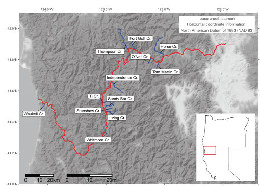
Main-stem Klamath River and both the natal (Scott and Shasta Rivers) and non-natal tributaries (see table 3), northern California. Note the Klamath River is truncated at 300 kilometers upstream from the mouth, just beyond the extent of the section considered in simulations.
Manhard and others (2018a) used conditional binomial models to estimate factors affecting the probability of fish immigrating into non-natal tributaries from the Klamath River. We used the approach detailed above in the S3 Model Structure section to convert from the conditional binomial probabilities used in Manhard and others (2018a) to unconditional multinomial probabilities. We used the second lowest AIC model from Manhard and others (2018a) that included maximum weekly decrease in discharge and the mean weekly temperature of the Klamath River at the mouth of each tributary as covariates (see Manhard and others, 2018a, for parameter estimates). This model describes factors that influence the summer entry into non-natal tributaries. To match the same scale as Manhard and others (2018a), we used the model to predict weekly immigration probabilities, then spread these probabilities evenly across the week to match the daily timestep of S3 dynamics during occupancy in the main stem river. The daily number of fish moving past tributary mouths are then multiplied by these daily non-natal immigration probabilities to simulate the number of fish entering each tributary from each upstream habitat unit. These fish are accumulated in each non-natal tributary as the simulation progresses, removing them from the main-stem Klamath River dynamics. Fish that do not enter non-natal tributaries continue with the full S3 simulation dynamics.
Next, we modeled winter and spring, where fish that have entered non-natal tributaries emigrate back into the main-stem Klamath River. We defined the winter emigration period as November 1–January 31 and relied on estimates of non-natal tributary survival from Manhard and others (2018a). To estimate the abundance of juvenile coho salmon surviving the winter period, we applied a mean annual survival rate (see table 22 in Manhard and others [2018a] for parameter estimates) corrected for the length of time spent in non-natal tributaries calculated as the median non-natal tributary entry date to the end of the winter emigration period. Next, we used the mean proportion of fish that emigrate over the winter period (see table 22 in Manhard and others [2018a] for parameter estimates, winter emigrant proportion) to simulate the number of fish leaving tributaries during the winter versus staying until the spring. Manhard and others (2018a) estimated the timing of fish emigrating from tributaries in relation to environmental covariates. To generalize the emigration timing for all non-natal tributaries in S3, we simplified the approach, relying on a subset of covariates from the lowest AIC model in Manhard and others (2018a). We used the intercept, representing the baseline emigration rate, and the slope term for weekly interval from Manhard and others (2018a) to estimate weekly conditional binomial probabilities. Because the S3 model runs on a daily time-step, we converted the weekly binomial probabilities used in Manhard and others (2018a) to daily, multinomial probabilities across the winter emigration period. As an example of converting from the conditional binomial probabilities to multinomial, given inputs to the binomial such as weekly mean day length representing photoperiod, we plotted an example along with the emigration probabilities for winter and spring periods (fig. 2). The emigration probabilities for winter peak in late December and early January.
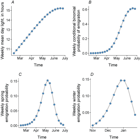
Elements defining weekly spring emigration probability of juvenile coho salmon (Oncorhynchus kisutch), including mean day light (A), conditional binomial probability (B), emigration probability (C), and weekly winter emigration probability (D). h, hours.
Next, we modeled the spring emigration period, defined as February 12–June 30. First, the remaining fish in each non-natal tributary survive (those that have not emigrated during the winter period). These fish are used to predict the abundance of fish available to emigrate during the spring period. We used the mean survival in non-natal tributaries (see table 22 in Manhard and others [2018a], for parameter estimates), corrected for the length of time from the end of the winter period to the end of the spring period. Next, the emigration timing was modeled using a subset of factors identified in the lowest AIC model from Manhard and others (2018a), including an intercept and a slope representing the effect of photoperiod. By using the intercept and photoperiod effect, this relationship can be easily generalized across all non-natal tributaries, allowing for expanding the number of non-natal tributaries in future applications of the model. We converted the predictions from weekly to daily multinomial probabilities across the spring emigration period. For the spring period, figure 2 shows an example of converting from the conditional binomial probabilities, based on inputs (hours of light, fig. 2A, for spring) to the multinomial probabilities. The spring emigration probability peaks in mid-May. Thus, the daily number of fish emigrating to the main-stem Klamath River was simply calculated as the total abundance of fish (calculated by applying the survival) multiplied by the daily emigration probability.
Because growth within non-natal tributaries was not simulated in S3, we estimated the monthly mean length of fish emigrating from tributaries to the main-stem Klamath using a large dataset of coho salmon size-at-date data. These measurements span a range of habitats and are similar to estimated sizes of emigrants from natal tributaries during overlapping periods. These mean monthly sizes of fish are applied to any fish emigrating from a tributary to the main-stem Klamath. Fish enter the Klamath River at their respective tributary mouths and the full set of S3 daily dynamics is then applied during the remainder of a simulation.
Mortality Submodel
Mortality in S3 is driven by three processes: (1) a baseline daily mortality rate, (2) water temperature, and (3) disease caused by C. shasta. A baseline daily survival rate of 0.921 for fry, parr, and smolts was used based on tagged coho salmon in the Klamath River (Beeman and others, 2012). We used the same water temperature mortality relationship as used for Chinook salmon (Perry, Plumb, and others, 2018) owing to similar upper incipient lethal temperatures for coho and Chinook salmon (McCullough and others, 2001). The disease submodel in S3 simulates the probability of becoming infected and eventually dying from C. shasta, given a time series of spore concentrations, the duration of exposure, and water temperatures. We adapted the survival cure model for S3 using the same approach as Perry and others (2019) but with updated parameters for coho salmon. We refer readers to Perry, Plumb, and others (2018) for the general structure and Perry and others (2019) for details on disease modeling dynamics. We only briefly describe the main components that were added or modified for our coho salmon application.
Fish within the Klamath River are infected by C. shasta within the infectious zone. The cure model components specify the probability of infection and eventual death (π), and the time-to-death for individuals that become infected, S(t|death). Within S3, we used the cure component of the model (π) to assign fish to a separate group of infected fish that are expected to eventually die. We then keep track of their time since infection and used the time-to-death component of the cure model “S(t|death)” to simulate the death of infected individuals as juveniles migrate downriver. Similar to Perry and others (2019), we applied constraints on some of the covariates to more closely match the conditions under which the cure model was developed. These included a maximum exposure time of 14 days and π = 0 for spore concentrations ≤ 1 spore/L.
In our coho salmon application including non-natal tributary dynamics, infected fish that are predicted to eventually die may move into non-natal tributaries. We allowed for this possibility and tracked these C. shasta related mortalities separately. We assumed that all infected fish that enter non-natal tributaries die and do not reenter the main-stem Klamath River. Additionally, some infected individuals may reach the ocean before they are predicted to die. We tracked these individuals and categorized them as C. shasta related mortalities given that they would be predicted to die had they remained within the bounds of the simulation. We report these three possible scenarios for C. shasta mortalities (in the Klamath River, in non-natal tributaries, and at the ocean) separately as both total numbers and summarize them as percentages (based on the total starting number of fish for each life history and source).
Results
Disease Model
Model selection proceeded in three steps for the mixture cure model (see “Disease Modelling” section). First, the generalized F distribution was the most highly supported distribution, based on AIC, for the time until death component of the mixture cure model (table 4). The log-logistic distribution was the next most highly supported model, but was greater than 2 ΔAIC from the generalized F. Second, in the survival timing portion of the model, the logarithm of spores was the most highly supported, by greater than 9 and 14 ΔAIC, from the full and main covariate model, respectively, compared to using just the spore concentration. We used the logarithm of spores in the survival timing portion of the model for further model fitting and selection. Third, we evaluated interactions by removing each individual interaction and only keeping interaction terms that reduced AIC by more than 10 units compared to the full model. This strategy resulted in only one interaction being kept, the exposure temperature and holding temperature interaction. Additionally, we kept the other main effects that included log spores, exposure temperature, holding temperature, and exposure duration.
Table 4.
Model selection results for coho salmon mixture cure models examining alternative distributions.[AIC: Akaike’s information criterion. ΔAIC: Difference between the model with the lowest AIC and the model being considered. k: Number of parameters in the model. LL: Log-likelihood]
The most highly supported mixture cure model generally was able to capture important elements of disease mortality dynamics of juvenile coho salmon infected with C. shasta (fig. 3). Comparing the Kaplan-Meier survival curves to the model predictions shows that the most highly supported model captured the delayed onset of mortality, the period of high mortality, and the plateau where mortality rate levels off. The model predicted higher mortality than was observed for several trials (numbers 7, 17, 24) and slightly lower mortality in several more (trial numbers 6, 10, 12). However, in general, the model captured patterns in mortality associated with fish infected with C. shasta. For the cure portion of the model that estimates the probability of infection and eventual death, the coefficients for C. Shasta spore concentration, exposure temperature, and exposure duration were positive (table 5). The coefficients for holding temperature and an interaction between exposure temperature and holding temperature were negative. In the time-to-death portion of the model, all coefficients representing covariate effects were negative, except an interaction term between exposure temperature and holding temperature, which was positive.

Kaplan-Meier survival curves and mixture cure model estimates from the most highly supported model for coho salmon (Oncorhynchus kisutch) sentinel trials. Numbers in the upper left corner of each graph represent the experimental trial number. d, days.
Table 5.
Parameter estimates from the survival cure model fitting to coho salmon (Oncorhynchus kisutch) sentinel experiments.[Model for π is a model for the proportion of fish that become infected and eventually die from ceratomyxosis. Model for S(t|death) is a model for the proportion of fish that survive to time t of those expected to die from C. shasta. Model terms: E, exposure duration; C, Ceratonova shasta spore concentration; TE, water temperature during exposure period; TH, water temperature during holding period. Symbols: --, no data]
We made predictions of survival probability across a range of covariates to illustrate the simultaneous effects of both portions of the mixture cure model on disease progression (fig. 4). Coho salmon are sensitive to even low spore concentrations, and across a range of other covariates, as the concentration of spores increased, the rate and overall mortality increased. The effects of elevated temperature on C. shasta mortality are clear—as temperature increases, mortality increases (moving down rows in fig. 4). Additionally, as exposure time increases, mortality increases across a range of spore concentrations.
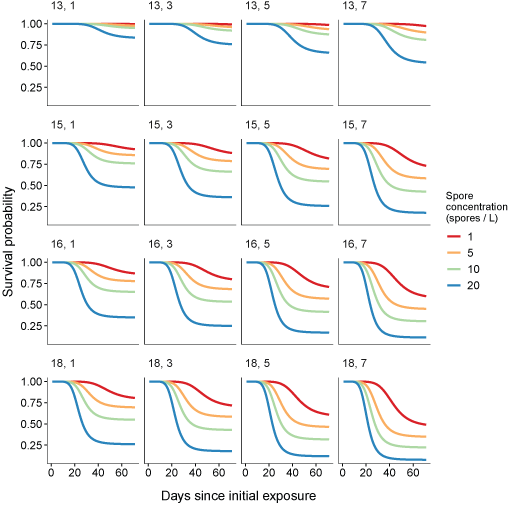
Predictions of survival probability over time from the most highly supported mixture cure model. Rows show a gradient in temperatures (top to bottom, 13, 15, 16, 18 degrees Celsius), columns show a range of exposure duration (left to right, 1, 3, 5, 7 days [d] exposure), and colors represent different spore concentrations (1, 5, 10, 20 genotype II spores per liter [spores/L]).
Model Inputs
Based on the models of Manhard and others (2018a), the peak of adult migration timing in the Scott River showed considerable variation between years, ranging from mid-October to late December (fig. 5A). Adult coho salmon migrating into the Shasta River showed less variation in timing between years, with the peak of migration typically occurring in mid-November to early December (fig. 5B).
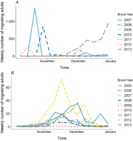
Simulated timing of adult coho salmon (Oncorhynchus kisutch) entering the Scott River to spawn (A) and Shasta River to spawn (B), northern California. Brood years represent the years adults spawn and produce offspring modeled in S3, not the years the adults were spawned.
For 7 brood years (2007–13), we calculated spring age-0, fall age-0, and spring age-1 fish entering the Klamath River from the Scott River (fig. 6). The peak for spring age-0 fish generally occurred in May and June, although the peak for spring age-1 fish was more variable, with peak abundance occurring from March through June in some years. Total abundance ranged from 434 in 2009 to 54,403 in 2007 (table 6).
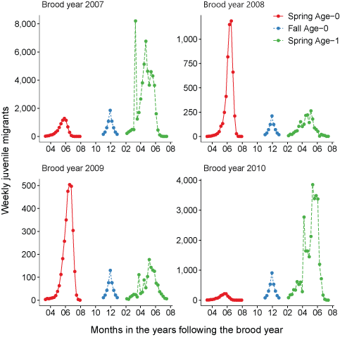
Simulated timing of juvenile coho salmon (Oncorhynchus kisutch) entering the main-stem Klamath River from the Scott River, northern California, brood years 2007–13. Coho salmon migrate during distinct periods as age-0 fish in the spring or fall and age-1 smolts in the spring.
Table 6.
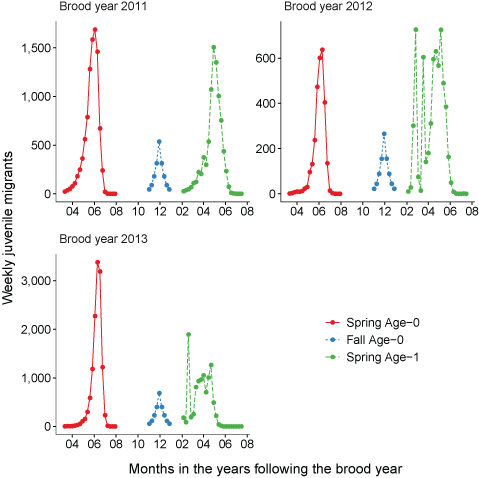
Total fish entering the Klamath River for each life history from the Scott River, northern California.Similarly, we calculated juvenile fish abundance and emigration timing from the Shasta River for 9 brood years from 2005 to 2013 (fig. 7). The peak for spring age-0 fish generally occurred in May and June; however, the peak was later in July during 2009 and 2010. Most spring age-1 fish generally migrated into the Klamath River in April and May. Total abundance of inputs from the Shasta River ranged from 54 in 2009 to 4,670 in 2007 (table 7).
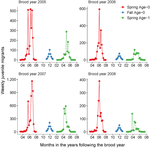

Simulated timing of juvenile coho salmon (Oncorhynchus kisutch) entering the main-stem Klamath River from the Shasta River, northern California, brood years 2005–13. Coho salmon migrate during distinct periods as age-0 fish in the spring or fall and age-1 smolts in the spring.
Table 7.
Total fish entering the Klamath River for each life history from the Shasta River, northern California.The mean total length across all brood years of fish entering the Klamath River from the Scott River was 56, and 109 mm for spring age-0, and spring age-1, respectively (fig. 8A). For the Shasta River, mean total length of migrating fish was 65, and 134 mm for spring age-0, and spring age-1, respectively (fig. 8B). Variation between years was caused by annual differences in temperature and ration levels that were used in the models to generate inputs for S3. Note the total length of fall age-0 fish was set to 90 mm.
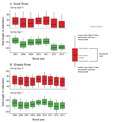
Mean total length (mm) for spring age-0 and age-1 migrating juvenile coho salmon (Oncorhynchus kisutch) from the Scott River for brood years 2007–13 (A) and the Shasta River for brood years 2005–13 (B), northern California.
Genotype II spore concentrations were variable among years, ranging from near zero to 50 spores per liter in 2015 (fig. 9). A noticeable peak in spore concentrations occurred in 2007, 2008, 2009, 2014, and 2015 with elevated concentrations typically during April, May, and June. In other years, spore concentrations were lower with the absence of any large peak of elevated concentrations.
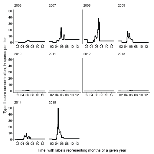
Daily Ceratonova shasta genotype II spore concentrations measured in the infectious zone, main-stem Klamath River, northern California.
Model Output
Tributary use by spring age-0 fish was variable, often depending on brood year and the location of non-natal tributaries (fig. 10A–10B). In general, non-natal tributaries farther upstream received the most use, and the number of fish entering tributaries decreased moving downstream. For Scott River fish, Tom Martin Creek had the highest use and for Shasta River fish, Horse Creek received the most fish. For a given non-natal tributary, the number of fish entering each year showed considerable variation. For instance, Scott River spring age-0 fish use of Tom Martin Creek varied by several thousand fish across brood years. Brood year 2010 had the lowest non-natal tributary use for Scott River fish with only 35 individuals simulated to enter. For Shasta River fish, brood year 2009 had the lowest non-natal tributary use.
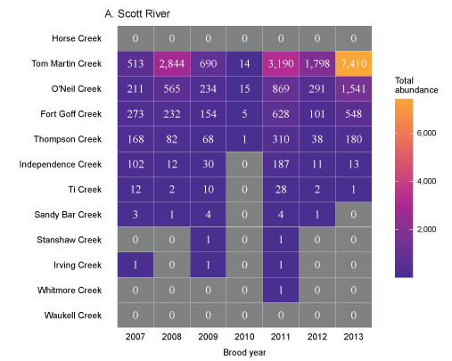
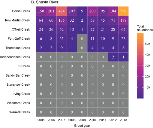
Total abundance of Scott River (A) and Shasta River (B) spring age-0 coho salmon (Oncorhynchus kisutch) entering non-natal tributaries from the main-stem Klamath River, northern California, for brood years 2007–13 and 2005–13, respectively. Tributaries are ordered from upstream (Horse Creek) to downstream (Waukell Creek).
Spring age-0 fish generally started entering non-natal tributaries in mid-May, with peak entry generally occurring in late June or early July (fig. 11; appendix 1). For some brood years, the start of entry was much later (mid-June or July). Entry into non-natal tributaries generally decreased by August. The entry timing was often unimodal; however, in several years the distributions of entry timing had multiple peaks.
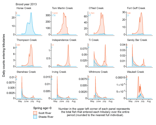
Simulated daily counts of coho salmon (Oncorhynchus kisutch) entering non-natal tributaries from the mainstem Klamath River, northern California, brood year 2013. Graphs are ordered (upper left to lower right, by rows) from downstream tributaries to upstream (see table 3). Note that the y-axis range varies among tributaries.
We present the population level impacts of C. shasta on coho salmon in several ways. First, using the fitted cure model and the S3 disease submodel, we track the daily percentage of infected fish passing Seiad Creek, typically considered the downstream boundary of the infectious zone (fig. 12). The percentage of infected fish showed considerable variation among years, with some years having high levels of infection (2007) and other years having low levels (2009; near 0 percent years omitted from figure). Infected spring age-0 fish started passing Seiad Creek in April and sustained high levels of infection during the summer months with infection rates generally decreasing by September. There were virtually no fall age-0 fish infected. Infected age-1 spring fish were primarily observed from the Shasta River. These fish started to pass Seiad Creek in April, continuing until September. Recall that our use of the term “infected” here refers to fish that become infected and eventually die at some point in time after infection, which is determined by the fitted cure model.
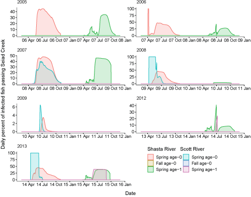
Daily percentage of fish infected with Ceratonova shasta passing Seiad Creek (river kilometer 215.3) in the Klamath River, northern California, brood years 2005–13. Years with near 0 percent infection are not shown. X-axis labels show two-digit migration year and month (08 Apr = April 2008). Note that the y-axis range varies among brood years.
Second, we track the daily percentage of infected fish entering the ocean (fig. 13). For some brood years and life histories, the percentage of infected fish entering the ocean was up to 40 percent (2005, 2007), while other brood years had a much lower percent entering the ocean (2009, years omitted from figure). Infected fish entering the ocean primarily consist of spring age-0 and age-1 life-histories, with virtually zero fall age-0 fish (table 8). Out of the spring age-1 life-history, fish from the Shasta River make up the dominant portion of infected fish entering the ocean.
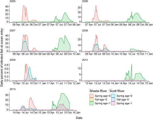
Daily percentage of fish infected with Ceratonova shasta at ocean entry in the Klamath River, northern California, brood years 2005–13. Years with near 0 percent infection are not shown. X-axis labels show two-digit migration year and month (08 Apr = April 2008). Note that the y-axis range varies among brood years.
Table 8.
Simulated number of coho salmon (Oncorhynchus kisutch) infected with Ceratonova shasta at ocean entry for each brood year, tributary source, and life-history strategy.[Groups with no infected individuals at ocean entry are omitted from the table]
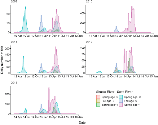
Third, to examine the overlap in timing between fish leaving the infectious zone and periods of peak spore concentrations, we present a series of paired plots showing the passage at Seiad Creek with the corresponding spore concentrations (fig. 14). In general, the passage timing of spring age-0 and age-1 fish overlapped with periods of elevated spore concentrations. For spring age-0 fish passing Seiad, this typically started in April or May and continued through the first 2 weeks of July. Age-1 fish from a given brood year, generally passed Seiad Creek during a more protracted period, the following calendar year, with a similar peak passage time as age-0 fish. Fall age-0 fish passed Seiad Creek starting in late fall until early spring, a period of low spore concentrations in the infectious zone.
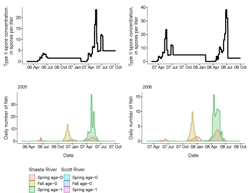
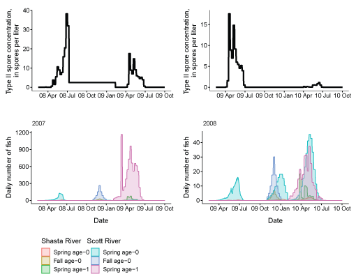

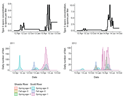

Genotype II Ceratonova shasta spore concentrations and daily number of coho salmon passing Seiad Creek (river kilometer 215.3) in the Klamath River, northern California, brood years 2005–13. X-axis labels show two-digit year and month (08 Apr = April 2008). Note the y-axis varies among graphs.
Fourth, we plot the number of in-river mortalities resulting from C. shasta as a function of river kilometer for each of the brood years considered (fig. 15). Mortality occurred across a wide range of river kilometers, however, most mortality occurred between river kilometers 150 and 250. Total number of in-river mortalities ranged from 0 in some years to 122 individuals from brood year 2007.
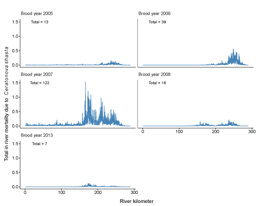
Spatial distribution of juvenile coho salmon (Oncorhynchus kisutch) in-river mortality due to Ceratonova shasta in the Klamath River, northern California, brood years 2005–13. Years not shown had near zero mortality. Text in the upper left of each graph shows the total number of in-river mortalities for a given brood year.
Lastly, we summarize percentage of mortality from C. shasta for each life-history strategy, source, and brood year (fig. 16). We stratify this percentage of mortality based on the simulated “fate” of infected individuals, including Klamath River, tributary (non-natal) and ocean. Most C. shasta-related mortality occurred in non-natal tributaries, where infected fish entered tributaries and were predicted to die. Infected fish that entered the ocean were the next largest source of C. shasta related mortality, particularly for spring age-1 fish from the Shasta River. These fish are smolts, actively migrating towards the ocean, and once infected in the infectious zone, have short travel times to the ocean. In-river mortality made up the smallest component, mostly affecting spring age-0 fish from the Shasta River. There were large differences in the percentage of mortality between natal tributaries and life histories. Overall, across all life histories, C. shasta mortality was lower in the Scott River than in the Shasta River, especially for spring age-1 fish. In both natal tributaries, fall age-0 fish had near zero mortality compared with spring age-0 or spring age-1 fish.
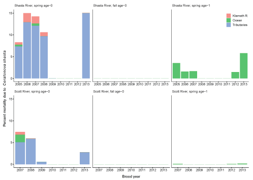
Percentage of mortality resulting from Ceratonova shasta for each life history and brood years 2005–13. Mortality is stratified by the location where individuals are simulated to die, including the Klamath River, ocean, and non-natal tributaries. Percentages are calculated as the number of fish simulated to die, stratified by location given the total starting number of fish from natal tributaries.
We simulated the daily number of coho salmon entering the ocean for each brood year and life history (fig. 17). The timing of ocean entry is similar across years for each life-history strategy. Age-0 spring fish generally showed three distinct peaks of ocean entry depending on the migratory pathway taken: (1) fish that remain in the main stem enter the ocean early during their first summer, (2) non-natal tributary use and winter emigration results in entry during winter as age-1 fish, and (3) spring emigration results in typical spring or summer ocean entry as age-1 smolts. Fall age-0 fish typically entered the ocean after a short residence in the main-stem Klamath River during winter from November through February. Spring age-1 fish entered over a longer time from March through June with most ocean entry finished by July.
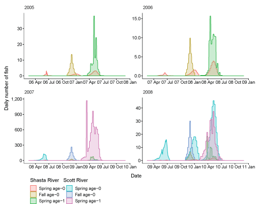
Daily number of coho salmon (Oncorhynchus kisutch) entering the ocean for each life history and brood years 2005–13. X-axis labels show two-digit year and month (08 Apr = April 2008). Note the y-axis varies among graphs.
We summarize these daily ocean entries as totals for each life history from the Scott and Shasta Rivers (fig. 18A–18B). The Scott River had higher abundance of juvenile coho salmon entering the ocean with abundance in the highest individual brood year (2007) topping 45,000 fish (combined across life histories). However, brood year 2007 stands out as having high production of fish, and in most years, abundance entering the ocean was considerably lower. Several hundred to several thousand fish produced from the Scott River was more typical. Spring age-1 fish generally accounted for most of the fish produced from the Scott River with lower numbers for both spring and fall age-0 fish.
The Shasta River produced lower numbers of fish reaching the ocean compared to the Scott River. The highest year for the Shasta River was brood year 2007 with more than 2,400 simulated to enter the ocean. Production of fish from brood year 2009 was particularly low, with only 133 fish simulated to reach the ocean. The number of fish representing each life-history strategy showed less variation in the Shasta River compared to the Scott River.
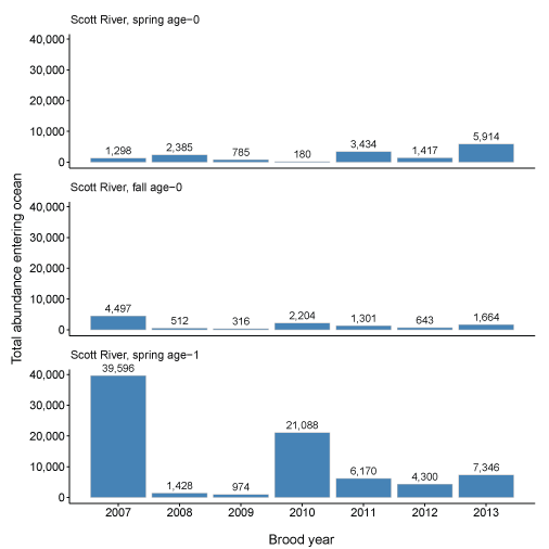
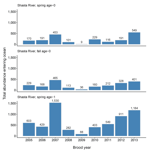
Total abundance of coho salmon (Oncorhynchus kisutch) entering the ocean for each brood year and life history for fish produced in the Scott River (A) and Shasta River (B), northern California, brood years 2007–13 and 2005–13, respectively.
Given the predictions of total fish entering the Klamath River and the abundance of fish entering the ocean, we calculated the percentage of fish surviving to ocean entry (fig. 19A–19B). These percentages generally reflect differences in life history, given various physical and biological inputs, and the time spent in the main-stem Klamath River and non-natal tributaries. For the Scott River, spring age-0 fish showed the most variation in survival from 13.8 to 50.1 percent, while survival for the other life histories was relatively constant. This pattern also was seen in Shasta River fish where most of the variation in survival was demonstrated by spring age-0 fish. Survival was lowest for spring age-0 fish from the Shasta River of any group considered, with survival to ocean entry ranging from 2.1 to 13.0 percent.
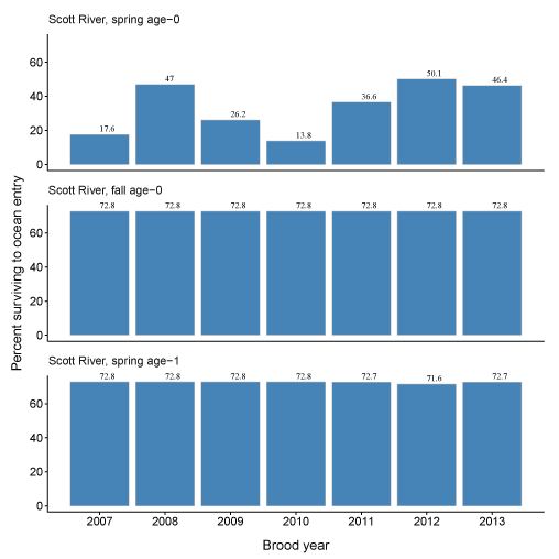
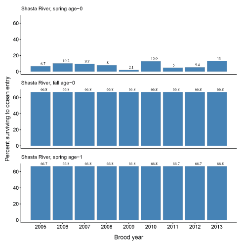
Percentage of coho salmon (Oncorhynchus kisutch) surviving to ocean entry for each brood year and life history from fish produced in the Scott River (A) and Shasta River (B), northern California, brood years 2007–13 and 2005–13, respectively.
Mean size at ocean entry was tracked in simulations, and boxplots of fork length of coho salmon smolts at ocean entry are shown in figure 20. The largest smolts at ocean entry were spring age-1 fish from the Shasta River. Spring age-1 fish from the Scott River were smaller and the mean size overlapped with the other life-history strategies in the Scott River. Spring age-0 fish from both rivers had considerable variation in the mean size at ocean entry with some fish entering around 90 mm fork length, whereas others entered close to 135 mm. Fall age-0 migrants showed little variation in size at ocean entry.
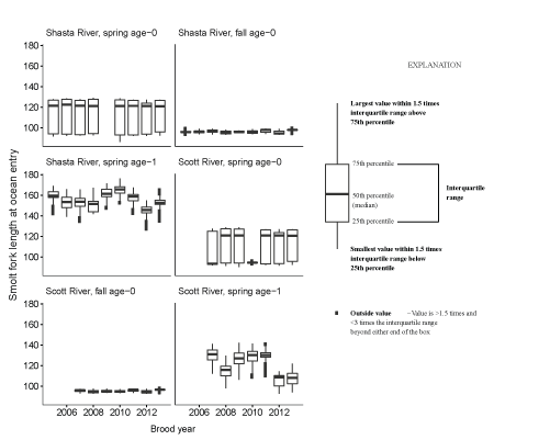
Fork length of coho salmon (Oncorhynchus kisutch) smolts at ocean entry for each source (Shasta River or Scott River) life history, and brood year.
We explore the effects of density dependent movement resulting from high densities of juvenile Chinook salmon in the main-stem Klamath River. To illustrate the effects, daily number of spring age-0 fish passing Seiad Creek were plotted with and without density dependent movement (Scott River, fig. 21; Shasta River, fig. 22). The effects of Chinook salmon densities generally were minor on the passage time at Seiad Creek.
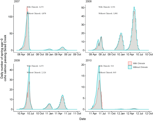
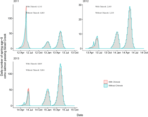
Daily number of fish passing Seiad Creek with Chinook salmon (Oncorhynchus tshawytscha) densities added to simulations and with simulations only containing coho salmon for fish from the Scott River, northern California, brood years 2007–13. Totals with and without the addition of Chinook salmon are shown over the entire time period. X-axis labels show two-digit year and month (12 Apr = April 2012). Note the y-axis varies among graphs.
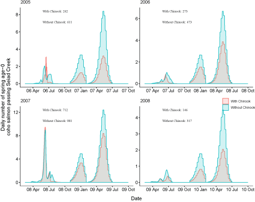
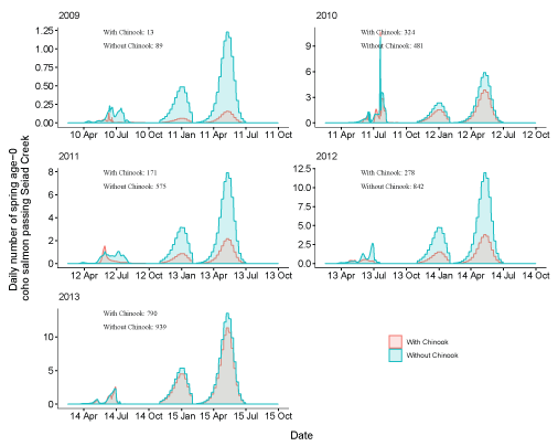
Daily number of fish passing Seiad Creek with Chinook salmon (Oncorhynchus tshawytscha) densities added to simulations and with simulations only containing coho salmon (Oncorhynchus kisutch) for fish from the Shasta River for brood years 2005–13. Totals with and without the addition of Chinook salmon are shown over the entire time period. X-axis labels show two-digit year and month (12 Apr = April 2012). Note the y-axis varies among graphs.
Total abundance of spring age-0 coho salmon entering the ocean for each brood year were simulated with and without Chinook salmon (fig. 23). The simulation with Chinook salmon resulted in fewer juvenile coho salmon reaching the ocean in all brood years. Generally, the differences in the number of coho salmon reaching the ocean with and without Chinook salmon were small for the Scott River source. There were some brood years (2005, 2011, 2012) where fish from the Shasta River more than doubled when Chinook salmon were removed from the simulations. The percentage of spring age-0 surviving to ocean entry also were simulated with and without Chinook salmon (fig. 24). The percentage of Scott River spring age-0 fish surviving to ocean entry showed similar patterns to the number entering the ocean. Shasta River spring age-0 fish showed the most variation among simulations with and without Chinook salmon. Without Chinook salmon, survival of Shasta River fish was higher, around 12 to almost 20 percent across years, compared with survival of less than 15 percent with Chinook salmon. In comparison, the survival to ocean entry was more similar for spring age-0 fish from the Scott River, although survival without Chinook salmon was higher in all years. The size of coho salmon smolts from both natal sources entering the ocean were similar with and without Chinook salmon in the simulations (fig. 25).
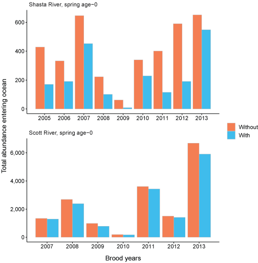
Total abundance entering ocean with Chinook salmon (Oncorhynchus tshawytscha) densities added to simulations (with) and with simulations only containing coho salmon (Oncorhynchus kisutch) (without) for spring age-0 fish from the Shasta and Scott Rivers, northern California, brood years 2005–13. Note the y-axis is different between graphs.
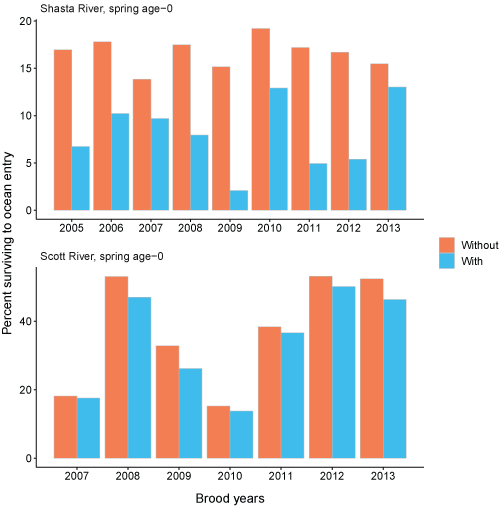
Percentage of spring age-0 surviving to ocean entry with Chinook salmon (Oncorhynchus tshawytscha) densities added to simulations (with) and with simulations only containing coho salmon (Oncorhynchus kisutch) (without) from the Shasta and Scott Rivers, northern California, brood years 2005–13. Note the y-axis is different between graphs.
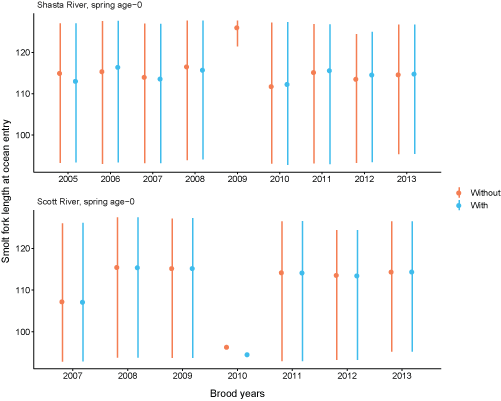
Average fork length of coho salmon (Oncorhynchus kisutch) smolts at ocean entry for spring age-0 fish from the Scott and Shasta Rivers, with and without Chinook salmon (Oncorhynchus tshawytscha) in the simulations, northern California, brood years 2005–13. Points represent the mean and the lines extend from the 20th to 80th percentiles.
Next, we compared the non-natal tributary use with and without Chinook salmon (figs. 26A–26B). For coho salmon from the Scott River, the non-natal tributary use without Chinook salmon was shifted downstream to some extent with more overall non-natal tributaries being used (compare fig. 26A with fig. 10A). Generally, the use of these tributaries by coho salmon increased without Chinook salmon, with higher total abundance predicted to enter non-natal tributaries. For fish from the Shasta River, non-natal tributary use without Chinook salmon shifted downstream slightly and the abundance of fish entering non-natal tributaries generally increased (compare fig. 26B with fig. 10B). The increased use of non-natal tributaries without Chinook salmon was most pronounced at upstream locations, particularly Horse and Tom Martin Creeks.
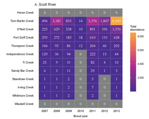
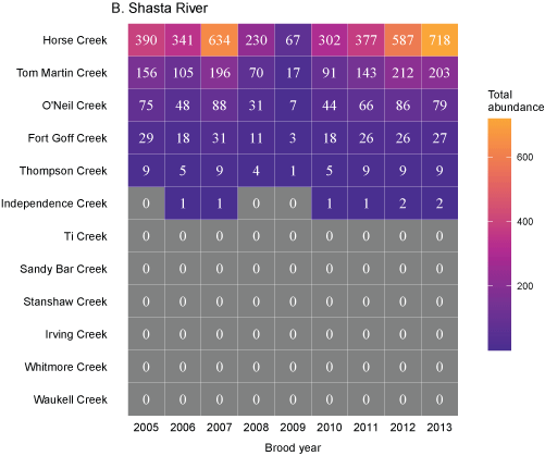
Total abundance of Scott River (A) and Shasta River (B) spring age-0 coho salmon (Oncorhynchus kisutch) entering non-natal tributaries from the main-stem Klamath River without Chinook salmon (Oncorhynchus tshawytscha) in the simulation, brood years 2007–13 and 2005–13, respectively. Tributaries are ordered from upstream (Horse Creek) to downstream (Waukell Creek).
Discussion
In this report. we extended the S3 modeling framework presented in earlier reports (Perry, Plumb, and others, 2018; Perry and others, 2019) to include coho salmon-specific dynamics with an emphasis on examining the population level impacts of C. shasta and variation in life-history strategy. Additionally, we considered simulations with and without juvenile Chinook salmon to explore the effects of density-dependent movement dynamics.
Using sentinel trials, we developed a model of how C. shasta affects juvenile coho salmon and incorporated this information into the S3 framework. Although survival cure models have been applied to coho salmon in prior work (Ray and others, 2014), we took advantage of genotype II specific spore concentrations and the inclusion of exposure duration. Coho salmon appear to be particularly susceptible to infection from genotype II spores, and our cure modeling shows high levels of infection and mortality at lower spore concentrations compared to Chinook salmon and genotype I. Coho salmon in trials responded similarly to prior work in respect to effects of temperature and C. shasta spore concentration (Ray and others, 2014). The inclusion of exposure duration was supported by our model selection approach and had significant coefficient estimates in both portions of the survival cure model. These results highlight the importance of exposure duration to understanding C. shasta disease dynamics in coho salmon, particularly for fish in the Klamath River Basin that may have varying levels of exposure.
The location of the Scott and Shasta Rivers with respect to the infectious zone provides a contrast to assess C. shasta related mortality from two main sources of juvenile coho salmon. The Scott River flows into the Klamath River roughly three-quarters of the way through the infectious zone, while fish originating from the Shasta River migrate through the entire infectious zone. Mortality resulting from C. shasta generally was higher for fish from the Shasta River than with fish from the Scott River. Our results are similar to Som and others (2019) that showed the predicted prevalence of mortality to be generally higher in a section of main-stem Klamath River from the Shasta River to Seiad Creek than with a section from the Scott River to Seiad Creek. Generally, migration timing for fish produced in both the Scott and Shasta Rivers overlapped with periods of higher spore concentrations in the main-stem Klamath River (except for fall age-0 fish). Because fish from both natal tributaries experience similar temperatures and spore concentrations, exposure duration likely contributed the most to simulated differences in C. shasta related mortality.
The different life-history strategies that we simulated had different levels of C. shasta related mortality, with spring age-0 fish having the highest mortality followed by spring age-1 fish and fall age-0 fish having near zero mortality. The timing of fall age-0 emigrating from the Scott and Shasta Rivers corresponds with low concentrations of spores in the main-stem Klamath River. Life-history diversity is often seen to provide stability to salmonid populations (Hilborn and others, 2003; Schindler and others, 2010). The fall age-0 strategy may confer some benefits to the Klamath River coho salmon population, especially in years with elevated spore concentrations. In some years, the spring age-1 fish from the Shasta River had elevated C. shasta related mortality. Because these fish are smolts that are actively migrating downstream, they are simulated to enter the ocean with ceratomyxosis. We have chosen to categorize these fish as C. shasta mortalities given that they would be predicted to die had they stayed within the simulation bounds. However, we acknowledge the uncertainty related to their ultimate fate as outside of the conditions used to develop and apply the survival cure model. Finally, we note that the issue of saltwater entry after onset of ceratomyxosis is currently being studied, and the results of those experiments will be incorporated into future versions of the S3 model.
The S3 model was developed to help resource managers weigh the potential costs and benefits of alternative management actions on juvenile salmonid populations. The model has been applied to examine restoration and water-management strategies on the Trinity and Klamath Rivers (Perry, Jones, and others, 2018; Perry and others, 2019). Here, we quantified the effects of C. shasta infection and mortality on juvenile coho salmon from the Scott and Shasta Rivers. Managed flow releases aimed to disturb habitat for the intermediate host of C. shasta (the annelid worm Manayunkia occidentalis) that releases the actinospore stage, which is infectious for salmon, have been implemented to reduce salmon mortality in the Klamath River Basin. To assess the impacts of these flows, Som and others (2019) developed models of prevalence of mortality, given disease relationships (see Ray and others, 2014), environmental data, and likely spore concentration changes to flows. Som and others (2019) found large variation in annual mortality rates across natal tributaries and years considered. Our results also showed large variation in simulated C. shasta related mortality between natal tributaries and years; however, the mortality rates generally were lower than Som and others (2019). The simulations did not include evaluation of proposed flow management aimed at decreasing spore concentrations, yet this type of evaluation could be incorporated into S3, providing additional lines of inference for evaluating flow-management actions. Additionally, hypotheses related to hatchery fish exacerbating C. shasta spores and potentially disease risk to naturally produced fish in the Klamath River Basin (Robinson and others, 2020) could be a fruitful area for the application of S3.
We explored the effects of density-dependent movement on coho salmon by including temporal and spatial Chinook salmon estimates from Perry and others (2019). Although density-dependent processes may manifest as changes in growth (Grant and Imre, 2005), survival (Einum and others, 2006), or movement (Hendrix and others, 2014), we focused on movement, because prior work supported density-dependent movement for Chinook salmon in the Klamath and Trinity Rivers (Perry and others, 2019). Passage timing at Seiad Creek was similar between the simulations with and without Chinook salmon. There were some differences in the total number of fish passing Seiad Creek. More coho salmon passed Seiad Creek in simulations without Chinook salmon in all simulations for the Scott River and Shasta River sources.
We also assessed the addition of Chinook salmon to simulations by calculating the number and percentage of survival of coho salmon at the ocean. In all simulations, the number and survival of coho salmon was higher without Chinook salmon. The largest effects of Chinook salmon were seen in coho salmon from the Shasta River, where in some brood years the abundance of coho salmon entering the ocean more than doubled and survival more than tripled. The abundance and survival of coho salmon from the Scott River showed smaller differences with the inclusion of Chinook salmon. Some of the variation between years, for the Scott River and Shasta River sources, was due to differences in the abundance of Chinook salmon among years (Perry and others, 2019) altering the strength of the density-dependent movement relationship. The higher abundance and survival at the ocean entry without Chinook salmon was due, in part, to increased non-natal tributary use by coho salmon, allowing fish to avoid high temperatures (leading to lower survival) in the main-stem Klamath River. The average size at ocean entry did not differ with or without Chinook salmon.
Significant caution should be exercised with interpreting the coho salmon results with the addition of Chinook salmon to S3 simulations as numerous factors were not considered in the current analysis that could ultimately affect the outcomes of these species interactions in the Klamath River. Although prior work has supported the inclusion of density-dependent movement in the Klamath and Trinity Rivers (Perry and others, 2019), density-dependent growth or survival could have a large influence on the simulation results. Recent work on salmonids (Grossman and Simon, 2020) suggests that density-dependent effects may manifest in numerous ways and future applications of S3 may consider density-dependent processes in growth and survival. Additionally, S3 could be used to examine the impacts of increased Chinook salmon densities on disease dynamics and C. shasta related mortality. Recent work by Robinson and others (2020) has shown that prevalence of infection in hatchery released Chinook salmon smolts is correlated with C. shasta spore concentrations in subsequent seasons. This relationship raises the question of whether hatchery releases of Chinook salmon may influence disease dynamics of the wild coho salmon population in the Klamath River Basin. Exploring these relationships between two species and the potential of increased Chinook salmon densities to influence coho salmon via altering disease dynamics is a fruitful area for future application of S3.
Increased densities of Chinook salmon in the main-stem Klamath River can potentially alter the non-natal tributary use by coho salmon. In general, non-natal tributary use by coho salmon increased without Chinook salmon. The use of non-natal tributaries also was shifted downstream to a limited extent. These shifts in non-natal tributary use were a product of differences in movement with and without Chinook salmon, and the environmental conditions influencing the probability of entering tributaries. An additional benefit of non-natal tributary use by coho salmon may be to avoid the high densities of Chinook salmon in the main-stem Klamath River and the associated competition or density-dependent effects.
Non-natal tributary use by coho salmon is one strategy to avoid unfavorable environmental conditions, particularly elevated temperatures in the Klamath River Basin (Sutton and Soto, 2012). Based on previous work by Manhard and others (2018a), we were able to simulate non-natal tributary use by spring age-0 fish in S3. Generally, upstream tributaries received the most use, especially O’Neil, Tom Martin, and Horse Creeks. The use of tributaries varied among years based on both the timing of fish leaving natal tributaries and the probability of entering a non-natal tributary (conditional on moving past a given tributary). Simulated spring age-0 fish that used non-natal tributaries and subsequently entered the main-stem Klamath River during the winter or spring periods had similar timing of ocean entry compared to fall age-0 and spring age-1 fish that did not use non-natal tributaries. Our efforts to simulate the non-natal tributary dynamics benefited from tagging efforts, and continued monitoring of tagged fish will help improve our understanding of these dynamics in the Klamath River Basin.
Coho salmon in the Klamath River show diversity in life-history strategies. Our simulations were structured to capture differences among spring age-0, fall age-0, and spring age-1 fish from the Scott and Shasta Rivers. Spring age-0 fish generally had higher mortality than fall age-0 and spring age-1 fish. As mentioned above, a component of this mortality for spring age-0 fish is related to disease, while fall age-0 fish in particular do not experience disease related mortality. Spring age-0 fish also show more variation in survival compared to either fall age-0 or spring age-1 fish. This is due to the various pathways that spring age-0 fish may experience including entering non-natal tributaries and out migrating from those tributaries during various times (winter versus spring). These differences in mortality contribute, in part, to differences in simulated abundance of fish entering the ocean. For the Scott River, abundance of fish entering the ocean was greater for spring age-1 fish than for spring age-0 fish in 6 of 7 brood years simulated. For the Shasta River, spring age-1 fish abundance was higher than spring age-0 fish abundance in all brood years simulated.
For spring age-0 fish, we observed variation in the mean size at ocean entry with some fish entering around 90 millimeters fork length and others entering at almost 135 mm. This variation was likely due to several factors including water temperatures in the main-stem Klamath River influencing growth, and the use of non-natal tributaries by spring age-0 fish. Fish that did not use non-natal tributaries entered the ocean at a younger age and smaller size than fish that spent additional time rearing in non-natal tributaries. Spring age-0 fish from the Scott and Shasta Rivers showed little difference in mean size at ocean entry. Spring age-1 fish from the Scott and Shasta Rivers showed more interannual variation in mean size at ocean entry. This variation was due in part to the models used to generate theses inputs to the main-stem Klamath River and the dynamics of the natal sources, the Scott and Shasta Rivers (Manhard and others, 2018a). Overall, differences in the size of fish at ocean entry can have important implications for marine growth and survival (Holtby and others, 1990).
The flow and temperatures regimes of the Klamath River Basin have undergone extensive modifications, both in the main-stem Klamath River and major tributaries, such as the Scott and Shasta Rivers. Water releases from Iron Gate Dam influence the downstream conditions for rearing coho salmon. In the Scott and Shasta Rivers, water withdrawals alter flows and water temperature regimes. The S3 model has the potential to address how changes in flow or temperature within these systems influences coho salmon. Changes in flow influence both the extent of available habitat in the main-stem Klamath River and production from the major tributaries. The impacts of alternative flow scenarios can be directly assessed using the S3 model. The impacts of alternative flow regimes on Chinook have been examined by Plumb and others (2019), yet there is a great potential to examine how flow alterations alter production of coho salmon in the Klamath River Basin.
There is an increasing recognition of the importance of water temperature regimes to the conservation of Pacific salmon because water temperature can influence many aspects of life history, development, and physiology. This is particularly true for coho salmon, as they experience thermal stress at temperatures as low as 16 °C (Brett, 1952). Temperature is incorporated into both survival and the bioenergetics submodels within S3. In addition, temperature drives the disease dynamics and C. shasta related mortality. These features make S3 useful for exploring how alternative management or environmental change likely will affect coho salmon production in the Klamath River Basin.
The application of S3 in the Klamath River has increased our understanding of several aspects of coho salmon population dynamics; however, this assessment is based on a set of assumptions and in some cases, limited data. For instance, we use survival estimates from Beeman and others (2012) that are based on tagged coho salmon smolts in the Klamath River. Although these estimates are from the species and river system of interest, we apply these rates to all life stages, which may not represent the typical increase in survival with size (Lorenzen, 1996). Although we recognize that estimating survival for earlier life stages may be challenging, empirical estimates of these rates would improve the realism of simulation methods such as S3.
Our understanding of movement rates of coho salmon in the Klamath River is limited and we used constant rates of movement for fry and parr during summer and winter periods (Manhard and others, 2018a). We used the mover-stayer model developed in previous applications of the S3 model (Perry, Plumb, and others, 2018) to model movement for fry and parr; however, we did not use the previous fish size based daily movement rates, but rather the movement rate was based on estimates from Manhard and others (2018a). The fish size and movement rate relationship used in prior applications is based on the average length-migration rate relationship obtained from Zabel (2002) and Plumb (2012) for juvenile Snake River fall Chinook salmon. We chose to use the seasonal movement rates estimated by Manhard and others (2018a) because these rates are based on coho salmon, the focal species of interest in our application, and these estimates were made in the Klamath River and tributaries. For the movement rates used in the mover-stayer model, we apply summer and winter rates that are constant for the time period. This was based on the best information available from tagging studies summarized in Manhard and others (2018a). Future studies aimed at refining our understanding of juvenile coho salmon movement dynamics in the Klamath River could incorporate individual level variation from factors such as fish size or life-stage or include environmental drivers, such as flow or temperature, that may influence movement rates. Once developed from field studies and tagging efforts, these types of relationships could be incorporated into the structure of S3, further refining the movement of individuals in the simulations.
To parametrize the advection-diffusion model used for smolts, we used information from coho salmon that had been radio tagged in the Klamath River (Beeman and others, 2012). This type of system and species-specific information is very useful for incorporating into simulation models such as S3. Additional information on movement of smolts and relationships with factors that may influence smolt movements would be valuable and could be incorporated into S3 to potentially improve the realism of simulations and ultimately benefit the management of salmonids in the Klamath River.
To model growth, we made the assumption that the proportion of maximum consumption in the Wisconsin bioenergetics model was 0.66, an assumption used in previous applications of S3 (Perry, Jones, and others, 2018; Perry and others, 2019), given the lack of empirical information on juvenile Chinook and coho salmon bioenergetics. Given this value, the Wisconsin (Stewart and Ibarra, 1991) and Ratkowsky growth models (Ratkowsky and others, 1983) predict similar growth over a range of temperatures (Perry, Plumb, and others, 2018). Additionally, the value of 0.66 implies that food availability does not limit growth of juveniles in the Klamath River and is consistent with the average value in the field reported by Armstrong and Schindler (2011). The current S3 model structure can accommodate variation in consumption between life stages and extending the model to account for spatial or temporal variation in consumption would be feasible. More complex and realistic characterizations of growth conditions would add additional realism to the simulation results produced by S3; however, this would require empirical research to characterize these sources of growth variation in the Klamath River and tributaries. Competition, turbidity, discharge, and prey availability can all influence growth in salmonids, ultimately influencing population dynamics (Korman and others, 2020). Additionally, in many temperate rivers, patterns in growth indicate seasonal changes, not only due to changes in water temperature, but to the phenology of production in rivers (Bernhardt and others, 2018). Investment in targeted field experiments or mechanistic modelling of consumption, such as in drift-foraging bioenergetics approaches, would likely pay dividends in our understanding of variation in growth and could be used in S3 to explore how this variation influences population dynamics.
Several key assumptions were made when considering non-natal tributary dynamics due to the limited availability of information to establish quantitative relationships. First, we are not aware of any weekly or monthly abundance or density estimates for the non-natal tributaries that we include in the simulation. Hence, an implicit assumption of our modeling is that these tributaries are not at carrying capacity to support fish moving from the main-stem Klamath River into non-natal tributaries. If information on the effect of fish densities on the probability of non-natal tributary entry were available, these dynamics could be included in S3. Similarly, if densities of either conspecifics or Chinook salmon in the main-stem Klamath River influenced the probability of entering a non-natal tributary due to some density dependent behavioral response, this type of dynamic could be included to improve the non-natal tributary dynamics. Although we were unable to include the above-mentioned effects, we did use available information on physical drivers of non-natal tributary use (Manhard and others, 2018a). If abundance or densities of coho salmon or Chinook salmon (or both species), were available at an appropriate temporal resolution in the main-stem Klamath River and in non-natal tributaries of interest, similar methods to those applied by (Manhard and others, 2018a) could be used to quantify these potentially important drivers of migratory behavior.
Based on tagged coho salmon in the Klamath River, we used a baseline daily survival rate of 0.921 for fry, parr, and smolts (Beeman and others, 2012). Although this estimate of survival is from coho salmon in the river system of interest, many species show a relationship between survival and fish size or age that we did not include. This may overestimate the survival for smaller fry and parr; however, we are unaware of any fish size and survival relationship for coho salmon in the Klamath River. An alternative would be to use a survival and fish size relationship from another species or another river system, yet we chose to use a constant survival rate for the focal species and system of interest, as this seemed most appropriate. We did include a temperature survival relationship, previously applied to Chinook salmon (Perry, Plumb, and others, 2018), owing to similarities in upper incipient lethal temperatures between the species (McCullough and others, 2001). The relationship between survival and temperature is based on data from Brett (1952) and fitting to this data by Perry, Plumb, and others (2018), which did not include life stage or fish size. If the interaction between these factors is of interest to managers, then further collections of field data or laboratory experiments would help to elucidate the relationship, which could be subsequently incorporated into future S3 simulations.
To simulate the fall age-0 life history, we made several assumptions including the magnitude of the emigrants and the timing of these fish leaving their natal rivers. These assumptions were necessary given the lack of monitoring data during the fall period. This life history strategy utilizes the main-stem Klamath River during a time of very low C. shasta spore concentrations, thereby avoiding mortality associated with disease in our simulations. Monitoring effort during this period in the Scott and Shasta Rivers would aid in evaluating these assumptions and potentially help to elucidate an important life-history strategy. Addressing these current limitations and prioritizing new data collection will improve the inferences gained from the application of S3 and ultimately could benefit management of coho salmon.
The current application of S3 to coho salmon has focused on the Scott and Shasta Rivers as natal sources of fish. This decision was partially based on the availability of data and the synthesis done by Manhard and others (2018a) resulting in methods to model spring age-0 and age-1 fish leaving these tributaries. Further model development could include other sources of fish, such as Bogus, Horse, and Seiad Creeks, if appropriate field datasets are collected and summarized providing the necessary inputs to S3. The inclusion of additional sources of coho salmon would likely influence the density-dependent movement dynamics we have incorporated, increasing the probability of moving for fry and parr. Increased movement may in turn influence the use of non-natal tributaries. Generally, the non-natal tributaries located farther upstream received the most use and this may be due, in part, to the location of the Scott and Shasta Rivers as sources. Adding additional sources of fish would likely increase the simulated use of non-natal tributaries located farther downstream. Additionally, we only included a limited number of non-natal tributaries, which could be expanded as well. Information on additional natal sources would surely help improve our understanding of non-natal tributary use and other important coho salmon dynamics in the Klamath River Basin.
References Cited
Alexander, J.D., Wright, K.A., Som, N.A., Hetrick, N.J., and Bartholomew, J.L. 2016. Integrating models to predict distribution of the invertebrate host of myxosporean parasites. Freshwater Science, v. 35, no. 4, p. 442–458, accessed July 18, 2022, at https://www.journals.uchicago.edu/doi/full/10.1086/688342.
Armstrong, J.B., and Schindler, D.E., 2011, Excess digestive capacity in predators reflects a life of feast and famine: Nature, v. 476, p. 84–87, accessed April 7, 2021, at https://www.nature.com/articles/nature10240.pdf.
Atkinson, S.D., and Bartholomew, J.L., 2010, Disparate infection patterns of Ceratomyxa shasta (Myxozoa) in rainbow trout (Oncorhynchus mykiss) and Chinook salmon (Oncorhynchus tshawytscha) correlate with internal transcribed spacer-1 sequence variation in the parasite: International Journal for Parasitology, v. 40, no. 5, p. 599–604, accessed April 7, 2021, at https://doi.org/10.1016/j.ijpara.2009.10.010.
Bartholow, J.M., 2005, Recent water temperature trends in the lower Klamath River, California: North American Journal of Fisheries Management, v. 25, no. 1, p. 152–162, accessed April 18, 2021, at https://doi.org/10.1577/M04-007.1.
Beacham, T.D., and Murray, C.B., 1990, Temperature, egg size, and development of embryos and alevins of five species of Pacific salmon—A comparative analysis: Transactions of the American Fisheries Society, v. 119, no. 6, p. 927–945, accessed April 18, 2021, at https://doi.org/10.1577/1548-8659(1990)119<0927:TESADO>2.3.CO;2.
Beacham, T.D., and Murray, C.B., 1993, Fecundity and egg size variation in North American Pacific salmon (Oncorhynchus): Journal of Fish Biology, v. 42, no. 4, p. 485–508, accessed April 7, 2021, at https://doi.org/10.1111/j.1095-8649.1993.tb00354.x.
Beeman, J., Juhnke, S., Stutzer, G., and Wright, K.2012, Effects of Iron Gate Dam discharge and other factors on the survival and migration of juvenile coho salmon in the lower Klamath River, northern California, 2006–09: U.S. Geological Survey Open-File Report 2012–1067, 96 p., accessed April 1, 2021, at https://doi.org/10.3133/ofr20121067.
Bernhardt, E.S., Heffernan, J.B., Grimm, N.B., Stanley, E.H., Harvey, J.W., Arroita, M., Appling, A.P., Cohen, M.J., McDowell, W.H., Hall, R.O., Jr., Read, J.S., Roberts, B.J., Stets, E.G., and Yackulic, C.B., 2018, The metabolic regimes of flowing waters: Limnology and Oceanography, v. 63, no. S1, p. S99–S118, accessed April 4, 2021, at https://doi.org/10.1002/lno.10726.
Brett, J.R., 1952, Temperature tolerance in young Pacific salmon, genus Oncorhynchus: Journal of the Fisheries Research Board of Canada, v. 9, no. 6, p. 265–323, accessed April 1, 2021, at https://doi.org/10.1139/f52-016.
Čada, G.F., Deacon, M.D., Mitz, S.V., and Bevelhimer, M.S., 1997, Effects of water velocity on the survival of downstream‐migrating juvenile salmon and steelhead—A review with emphasis on the Columbia River Basin: Reviews in Fisheries Science, v. 5, no. 2, p. 131–183, accessed April 27, 2021, at https://doi.org/10.1080/10641269709388596.
Chesney, D., and Knechtle, M., 2015, Shasta River Chinook and coho salmon observations in 2014, Siskiyou County, CA—Final report: Yreka, California, California Department of Fish and Wildlife, Klamath River Project, 26 p, accessed April 3, 2021, at https://kbifrm.psmfc.org/wp-content/uploads/2017/01/Chesney-et-al_2015_0040_2014-Shasta-River-final-report.pdf.
Einum, S., Sundt‐Hansen, L., and Nislow, K.H., 2006, The partitioning of density‐dependent dispersal, growth and survival throughout ontogeny in a highly fecund organism: Oikos, v. 113, no. 3, p. 489–496, accessed April 3, 2021, at https://doi.org/10.1111/j.2006.0030-1299.14806.x.
Fausch, K.D., 1988, Tests of competition between native and introduced salmonids in streams—What have we learned?: Canadian Journal of Fisheries and Aquatic Sciences, v. 45, no. 12, p. 2238–2246, accessed April 7, 2021, at https://doi.org/10.1139/f88-260.
Federal Register, 1997, Endangered and threatened species; threatened status for Southern Oregon/Northern California Coast Evolutionarily Significant Unit of coho salmon: Federal Register, v. 62, p. 24588–24609, accessed August 2, 2022, at https://www.federalregister.gov/documents/1997/05/06/97-11571/endangered-and-threatened-species-threatened-status-for-southern-oregonnorthern-california-coast.
Fujiwara, M., Mohr, M.S., Greenberg, A., Foott, J.S., and Bartholomew, J.L., 2011, Effects of Ceratomyxosis on population dynamics of Klamath fall-run Chinook salmon: Transactions of the American Fisheries Society, v. 140, no. 5, p. 1380–1391, accessed April 3, 2021, at https://doi.org/10.1080/00028487.2011.621811.
Giudice, D., and Knechtle, M., 2019, Shasta River salmonid monitoring 2018, Siskiyou County, CA: Yreka, California, California Department of Fish and Wildlife, Klamath River Project, 28 p., accessed April 7, 2021, at https://nrm.dfg.ca.gov/FileHandler.ashx?DocumentID=174881.
Grant, J.W.A., and Imre, I., 2005, Patterns of density‐dependent growth in juvenile stream‐dwelling salmonids: Journal of Fish Biology, v. 67, p. 100–110, accessed April 3, 2021, at https://doi.org/10.1111/j.0022-1112.2005.00916.x.
Grossman, G.D., and Simon, T.N., 2020, Density‐dependent effects on salmonid populations—A review: Ecology of Freshwater Fish, v. 29, no. 3, p. 400–418, accessed April 7, 2021, at https://doi.org/10.1111/eff.12523.
Hallett, S.L., and Bartholomew, J.L., 2006, Application of a real-time PCR assay to detect and quantify the myxozoan parasite Ceratomyxa shasta in river water samples: Diseases of Aquatic Organisms, v. 71, no. 2, p. 109–118, accessed April 3, 2021, at https://doi.org/10.3354/dao071109.
Hallett, S.L., Ray, R.A., Hurst, C.N., Holt, R.A., Buckles, G.R., Atkinson, S.D., and Bartholomew, J.L., 2012, Density of the waterborne parasite Ceratomyxa shasta and its biological effects on salmon: Applied and Environmental Microbiology, v. 78, no. 10, p. 3724–3731, accessed April 7, 2021, at https://doi.org/10.1128/AEM.07801-11.
Hearn, W.E., 1987, Interspecific competition and habitat segregation among stream‐dwelling trout and salmon—A review: Fisheries, v. 12, no. 5, p. 24–31, accessed April 1, 2021, at https://doi.org/10.1577/1548-8446(1987)012<0024:ICAHSA>2.0.CO;2.
Hendrix, N., Criss, A., Danner, E., Greene, C.M., Imaki, H., Pike, A., and Lindley, S.T., 2014, Life cycle modeling framework for Sacramento River winter-run Chinook salmon: National Oceanic and Atmospheric Administration technical memorandum, NOAA-TM-NMFS-SWFSC-530, accessed April 7, 2021, at https://swfsc-publications.fisheries.noaa.gov/publications/TM/SWFSC/NOAA-TM-NMFS-SWFSC-530.pdf.
Hilborn, R., Quinn, T.P., Schindler, D.E., and Rogers, D.E., 2003, Biocomplexity and fisheries sustainability: Proceedings of the National Academy of Sciences of the United States of America, v. 100, no. 11, p. 6564–6568, accessed April 7, 2021, at https://doi.org/10.1073/pnas.1037274100.
Holtby, L.B., Andersen, B.C., and Kadowaki, R.K., 1990, Importance of smolt size and early ocean growth to interannual variability in marine survival of coho salmon (Oncorhynchus kisutch): Canadian Journal of Fisheries and Aquatic Sciences, v. 47, no. 11, p. 2181–2194, accessed April 27, 2021, at https://cdnsciencepub.com/doi/pdf/10.1139/f90-243.
Hurst, C.N., and Bartholomew, J.L., 2012, Ceratomyxa shasta genotypes cause differential mortality in their salmonid hosts: Journal of Fish Diseases, v. 35, no. 10, p. 725–732, accessed April 7, 2021, at https://doi.org/10.1111/j.1365-2761.2012.01407.x.
Knechtle, M., and Chesney, D., 2016, 2015 Scott River salmon studies—Final report: Yreka, California, California Department of Fish and Wildlife, Klamath River Project, 27 p., accessed April 3, 2021, at https://kbifrm.psmfc.org/wp-content/uploads/2017/01/Knechtle-et-al_2016_0038_2015-Scott-River-river-salmon-studies-final-report.pdf.
Knechtle, M., and Giudice, D., 2019, 2018 Scott River salmon studies—Final report: Yreka, California, California Department of Fish and Wildlife, Klamath River Project, 26 p., accessed April 3, 2021, at https://nrmsecure.dfg.ca.gov/FileHandler.ashx?DocumentID=174880.
Korman, J., Yard, M.D., Dzul, M.C., Yackulic, C.B., Dodrill, M.J., Deemer, B.R., and Kennedy, T.A., 2020, Changes in prey, turbidity, and competition reduce somatic growth and cause the collapse of a fish population: Ecological Monographs, v. 91, no. 1, 20 p., accessed April 3, 2021, at https://doi.org/10.1002/ecm.1427.
Lestelle, L.C., 2007, Coho salmon (Oncorhynchus kisutch) life history patterns in the Pacific Northwest and California—Final report: Prepared for Bureau of Reclamation, Klamath Area Office, 143 p., accessed April 7, 2021, at http://www.defendruralamerica.com/files/LestelleReport.pdf.
Lister, D., and Genoe, H., 1970, Stream habitat utilization by cohabiting underyearlings of chinook (Oncorhynchus tshawytscha) and coho (O. kisutch) salmon in the Big Qualicum River, British Columbia: Journal of the Fisheries Research Board of Canada, v. 27, no. 7, p. 1215–1224, accessed April 1, 2021, at https://doi.org/10.1139/f70-144.
Lorenzen, K., 1996, The relationship between body weight and natural mortality in juvenile and adult fish—A comparison of natural ecosystems and aquaculture: Journal of Fish Biology, v. 49, no. 4, p. 627–642, accessed April 17, 2021, at https://doi.org/10.1111/j.1095-8649.1996.tb00060.x.
Manhard, C.V., Som, N.A., Perry, R.W., Faukner, J.R., and Soto, T., 2018a, Estimating freshwater productivity, overwinter survival, and migration patterns of Klamath River coho salmon: Arcata, California, U.S. Fish and Wildlife Service, Arcata Fish and Wildlife Office, Arcata Fisheries Technical Report TR 2018-33, 84 p., accessed April 7, 2021, at https://www.fws.gov/media/estimating-freshwater-productivity-overwinter-survival-and-migration-patterns-klamath-river.
Manhard, C.V., Som, N.A., Perry, R.W., and Plumb, J.M., 2018b, A laboratory-calibrated model of coho salmon growth with utility for ecological analyses: Canadian Journal of Fisheries and Aquatic Sciences, v. 75, no. 5, p. 682–690, accessed April 3, 2021, at https://doi.org/10.1139/cjfas-2016-0506.
McCullough, D., Spalding, S., Sturdevant, D., and Hicks, M., 2001, Summary of technical literature examining the physiological effects of temperature on salmonids: Seattle, Washington, U.S. Environmental Protection Agency Report EPA-910-D-01-005, accessed April 3, 2021, at https://nepis.epa.gov/Exe/tiff2png.cgi/P100LVKL.PNG?-r+75+-g+7+D%3A%5CZYFILES%5CINDEX%20DATA%5C00THRU05%5CTIFF%5C00002203%5CP100LVKL.TIF.
National Research Council, 2004, Endangered and threatened fishes in the Klamath River Basin—Causes of decline and strategies for recovery: Washington D.C., The National Academies Press, accessed April 7, 2021, at https://doi.org/10.17226/10838.
Nichols, A., Willis, A., Jeffres, C., and Deas, M., 2014, Water temperature patterns below large groundwater springs—Management implications for coho salmon in the Shasta River, California: River Research and Applications, v. 30, no. 4, p. 442–455, accessed April 7, 2021, at https://doi.org/10.1002/rra.2655.
Perry, R.W., Jones, E.C., Plumb, J.M., Som, N.A., Hetrick, N.J., Hardy, T.B., Polos, J.C., Martin, A.C., Alvarez, J.S., and De Juilio, K.P., 2018, Application of the Stream Salmonid Simulator (S3) to the restoration reach of the Trinity River, California—Parameterization and calibration: U.S. Geological Survey Open-File Report 2018–1174, 65 p., accessed April 27, 2021, at https://doi.org/10.3133/ofr20181174.
Perry, R.W., Plumb, J.M., Jones, E.C., Som, N.A., Hardy, T.B., and Hetrick, N.J., 2019, Application of the Stream Salmonid Simulator (S3) to Klamath River fall Chinook salmon (Oncorhynchus tshawytscha), California—Parameterization and calibration: U.S. Geological Survey Open-File Report 2019–1107, 89 p., accessed April 7, 2021, at https://doi.org/10.3133/ofr20191107.
Perry, R.W., Plumb, J.M., Jones, E.C., Som, N.A., Hetrick, N.J., and Hardy, T.B., 2018, Model structure of the Stream salmonid simulator (S3)—A dynamic model for simulating growth, movement, and survival of juvenile salmonids: U.S. Geological Survey Open-File Report 2018–1056, 32 p., accessed April 7, 2021, at https://doi.org/10.3133/ofr20181056.
Perry, R.W., Risley, J.C., Brewer, S.J., Jones, E.C., and Rondorf, D.W., 2011, Simulating water temperature of the Klamath River under dam removal and climate change scenarios: U.S. Geological Survey Open-File Report 2011–1243, 78 p., accessed April 1, 2021, at https://pubs.usgs.gov/of/2011/1243/.
Plumb, J.M., 2012, Evaluation of models and the factors affecting the migration and growth of naturally-produced subyearling fall Chinook salmon (Oncorhynchus tshawytscha) in the Lower Snake River: Moscow, Idaho, University of Idaho, Ph.D. dissertation, 171 p., accessed April 7, 2021, at https://www.researchgate.net/publication/259601672_EVALUATION_OF_MODELS_AND_THE_FACTORS_AFFECTING_THE_MIGRATION_AND_GROWTH_OF_NATURALLY-PRODUCED_SUBYEARLING_FALL_CHINOOK_SALMON_ONCORHYNCHUS_TSHAWYTSCHA_IN_THE_LOWER_SNAKE_RIVER.
Plumb, J.M., Perry, R.W., Som, N.A., Alexander, J., and Hetrick, N.J., 2019, Using the stream salmonid simulator (S3) to assess juvenile Chinook salmon (Oncorhynchus tshawytscha) production under historical and proposed action flows in the Klamath River: California: U.S. Geological Survey Open File Report 2019–1099, 43 p., accessed April 3, 2021, at https://doi.org/10.3133/ofr20191099.
R Core Team, 2019, R—A language and environment for statistical computing: Vienna, Austria, R Foundation for Statistical Computing, accessed April 1, 2021, at https://www.R-project.org/.
Ratkowsky, D.A., Lowry, R.K., McMeekin, T.A., Stokes, A.N., and Chandler, R.E., 1983, Model for bacterial culture growth rate throughout the entire biokinetic temperature range: Journal of Bacteriology, v. 154, no. 3, p. 1222–1226, accessed April 23, 2021, at https://doi.org/10.1128/jb.154.3.1222-1226.1983.
Ray, R.A., Holt, R.A., and Bartholomew, J.L., 2012, Relationship between temperature and Ceratomyxa shasta-induced mortality in Klamath River salmonids: The Journal of Parasitology, v. 98, no. 3, p. 520–526, accessed April 7, 2021, at https://doi.org/10.1645/JP-GE-2737.1.
Ray, R.A., Perry, R.W., Som, N.A., and Bartholomew, J.L., 2014, Using cure models for analyzing the influence of pathogens on salmon survival: Transactions of the American Fisheries Society, v. 143, no. 2, p. 387–398, accessed April 3, 2021, at https://doi.org/10.1080/00028487.2013.862183.
Robinson, H.E., Alexander, J.D., Hallett, S.L., and Som, N.A., 2020, Prevalence of infection in hatchery‐origin Chinook salmon correlates with abundance of Ceratonova shasta spores—Implications for management and disease risk: North American Journal of Fisheries Management, v. 40, no. 4, p. 959–972, accessed April 7, 2021, at https://doi.org/10.1002/nafm.10456.
Schindler, D.E., Hilborn, R., Chasco, B., Boatright, C.P., Quinn, T.P., Rogers, L.A., and Webster, M.S., 2010, Population diversity and the portfolio effect in an exploited species: Nature, v. 465, no. 7298, p. 609–612, accessed April 1, 2021, at https://doi.org/10.1038/nature09060.
Shea, C., Hetrick, N.J., and Som, N.A. 2016. Response to request for technical assistance – sediment mobilization and flow history in Klamath River below Iron Gate Dam. Technical memorandum. U.S. Fish and Wildlife Service, Arcata Fish and Wildlife Office, Arcata, California, USA, accessed August 8, 2022, at https://kbifrm.psmfc.org/file/response-to-request-for-technical-assistance-sediment-mobilization-and-flow-history-in-klamath-river-below-iron-gate-dam.
Som, N.A., Hetrick, N.J., Perry, R., and Alexander, J.D., 2019, Estimating annual Ceratonova shasta mortality rates in juvenile Scott and Shasta River coho salmon that enter the Klamath River main stem: U.S. Fish and Wildlife Service, Arcata fisheries technical report number TR 2019-28, 18 p., accessed April 3, 2021, at https://pubs.er.usgs.gov/publication/70206402
Spence, B.C., and Dick, E.J., 2014, Geographic variation in environmental factors regulating outmigration timing of coho salmon (Oncorhynchus kisutch) smolts: Canadian Journal of Fisheries and Aquatic Sciences, v. 71, no. 1, p. 56–69, accessed April 7, 2021, at https://doi.org/10.1139/cjfas-2012-0479.
Stein, R.A., Reimers, P.E., and Hall, J.D., 1972, Social interaction between juvenile coho (Oncorhynchus kisutch) and fall Chinook salmon (O. tshawytscha) in Sixes River, Oregon: Journal of the Fisheries Research Board of Canada, v. 29, no. 12, p. 1737–1748, accessed April 3, 2021, at https://doi.org/10.1139/f72-275.
Stewart, D.J., and Ibarra, M., 1991, Predation and production by salmonine fishes in Lake Michigan, 1978–88: Canadian Journal of Fisheries and Aquatic Sciences, v. 48, no. 5, p. 909–922, accessed April 27, 2021, at https://doi.org/10.1139/f91-107.
Stinson, M.E., Atkinson, S.D., and Bartholomew, J.L., 2018, Widespread distribution of Ceratonova shasta (Cnidaria—Myxosporea) genotypes indicates evolutionary adaptation to its salmonid fish hosts: The Journal of Parasitology, v. 104, no. 6, p. 645–650, accessed April 3, 2021, at https://doi.org/10.1645/18-79.
Sutton, R., and Soto, T., 2012, Juvenile coho salmon behavioural characteristics in Klamath river summer thermal refugia: River Research and Applications, v. 28, no. 3, p. 338–346, accessed April 23, 2021, at https://doi.org/10.1002/rra.1459.
Sutton, R.J., Deas, M.L., Tanaka, S.K., Soto, T., and Corum, R.A., 2007, Salmonid observations at a Klamath River thermal refuge under various hydrological and meteorological conditions: River Research and Applications, v. 23, no. 7, p. 775–785, accessed April 3, 2021, at https://doi.org/10.1002/rra.1026.
Witmore, S.K., 2014, Seasonal growth, retention, and movement of juvenile coho salmon in natural and constructed habitats of the mid-Klamath River: Arcata, California, Humboldt State University, Master’s thesis, 83 p., accessed April 7, 2021, at https://scholarworks.calstate.edu/concern/theses/6d56zz89d.
Zabel, R.W., 2002, Using “travel time” data to characterize the behavior of migrating animals: American Naturalist, v. 159, no. 4, p. 372–387, accessed April 27, 2021, at https://doi.org/10.1086/338993.
Zabel, R.W., and Anderson, J.J., 1997, A model of the travel time of migrating juvenile salmon, with an application to Snake River spring chinook salmon: North American Journal of Fisheries Management, v. 17, no. 1, p. 93–100, accessed April 7, 2021, at https://doi.org/10.1577/1548-8675(1997)017<0093:AMOTTT>2.3.CO;2.
Zhang, J., and Peng, Y., 2007, A new estimation method for the semiparametric accelerated failure time mixture cure model: Statistics in Medicine, v. 26, no. 16, p. 3157–3171, accessed April 1, 2021, at https://doi.org/10.1002/sim.2748.
Appendix 1. Simulated Daily Counts of Coho Salmon Entering Tributaries from the Main-Stem Klamath River
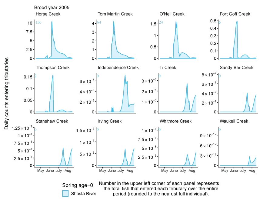
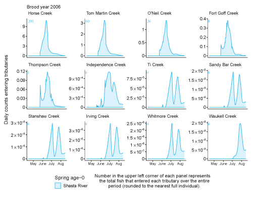

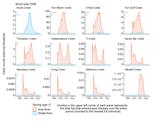
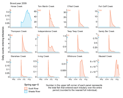
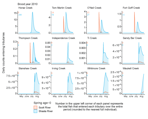


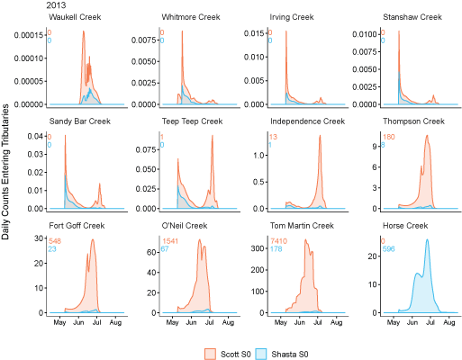
Graphs showing simulated daily counts of coho salmon (Oncorhynchus kisutch) entering tributaries from the main-stem Klamath River, northern California, brood years 2005–13. Only the spring age-0 migrants from the Scott and Shasta Rivers are shown. Number(s) in upper left of each graph represents the total fish that entered each tributary over the entire period (rounded to the nearest full individual). Panels are ordered (upper left to lower right, by rows) from downstream tributaries to upstream (see table 3). Note the y-axis varies among graphs.
Conversion Factors
Datums
Vertical coordinate information is referenced to North American Vertical Datum of 1988 (NAVD 88).
Horizontal coordinate information is referenced to the North American Datum of 1983 (NAD 83).
For information about the research in this report, contact
Director, Western Fisheries Research Center
U.S. Geological Survey
6505 NE 65th Street
Seattle, Washington 98115-5016
https://www.usgs.gov/centers/western-fisheries-research-center
Manuscript approved on July 26, 2022
Publishing support provided by the U.S. Geological Survey
Science Publishing Network, Tacoma Publishing Service Center
Suggested Citation
Dodrill, M.J., Perry, R.W., Som, N.A., Manhard, C.V., and Alexander, J.D., 2022, Extending the Stream Salmonid Simulator to accommodate the life history of coho salmon (Oncorhynchus kisutch) in the Klamath River Basin, Northern California: U.S. Geological Survey Open-File Report 2022–1071, 70 p., https://doi.org/10.3133/ofr20221071.
ISSN: 2331-1258 (online)
Study Area
| Publication type | Report |
|---|---|
| Publication Subtype | USGS Numbered Series |
| Title | Extending the Stream Salmonid Simulator to accommodate the life history of coho salmon (Oncorhynchus kisutch) in the Klamath River Basin, Northern California |
| Series title | Open-File Report |
| Series number | 2022-1071 |
| DOI | 10.3133/ofr20221071 |
| Year Published | 2022 |
| Language | English |
| Publisher | U.S. Geological Survey |
| Publisher location | Reston, VA |
| Contributing office(s) | Western Fisheries Research Center |
| Description | viii, 70 p. |
| Country | United States |
| State | California |
| Other Geospatial | Klamath River basin |
| Online Only (Y/N) | Y |
| Google Analytic Metrics | Metrics page |