

A Summary of Water-Quality and Salt Marsh Monitoring, Humboldt Bay, California
Links
- Document: Report (12 MB pdf) , HTML , XML
- Data Releases:
- Model archive summary for a suspended-sediment concentration surrogate regression model for station 404038124131801; Hookton Slough near Loleta, CA
- Model archive summary for a suspended-sediment concentration surrogate regression model for station 405219124085601; Mad River Slough near Arcata, CA
- Salt marsh monitoring during water years 2013 to 2019, Humboldt Bay, CA—Water levels, surface deposition, elevation change, and soil carbon storage
- Download citation as: RIS | Dublin Core
Acknowledgments
The U.S. Geological Survey Humboldt Bay Water Quality and Salt Marsh Monitoring Program was designed and completed in cooperation with the California State Coastal Conservancy, California Department of Fish and Wildlife, and the U.S. Fish and Wildlife Service—Humboldt Bay National Wildlife Refuge.
Abstract
This report summarizes data-collection activities associated with the U.S. Geological Survey Humboldt Bay Water-Quality and Salt Marsh Monitoring Project. This work was undertaken to gain a comprehensive understanding of water-quality conditions, salt marsh accretion processes, marsh-edge erosion, and soil-carbon storage in Humboldt Bay, California. Multiparameter sondes recorded water temperature, specific conductance, and turbidity at a 15-minute timestep at two U.S. Geological Survey water-quality stations: (1) Mad River Slough near Arcata, California (U.S. Geological Survey station 405219124085601) and (2) Hookton Slough near Loleta, California (U.S. Geological Survey station 404038124131801). At each station, discrete water samples were collected to develop surrogate regression models that were used to compute a continuous time series of suspended-sediment concentration from continuously measured turbidity. Data loggers recorded water depth at a 6-minute timestep in the primary tidal channels (Mad River Slough and Hookton Slough) in two adjacent marshes (Mad River marsh and Hookton marsh). The marsh monitoring network included five study marshes. Three marshes (Mad River, Manila, and Jacoby) are in the northern embayment of Humboldt Bay and two marshes (White and Hookton) are in the southern embayment. Surface deposition and elevation change were measured using deep rod surface elevation tables and feldspar marker horizons. Sediment characteristics and soil-carbon storage were measured using a total of 10 shallow cores, distributed across 5 study marshes, collected using an Eijkelkamp peat sampler. Rates of marsh edge erosion (2010–19) were quantified in four marshes (Mad River, Manila, Jacoby, and White) by estimating changes in the areal extent of the vegetated marsh plain using repeat aerial imagery and light detection and ranging (LiDAR)-derived elevation data. During the monitoring period (2016–19), the mean suspended-sediment concentration computed for Hookton Slough (50±20 milligrams per liter [mg/L]) was higher than Mad River Slough (18±7 mg/L). Uncertainty in mean suspended-sediment concentration values is reported using a 90-percent confidence interval. Across the five study marshes, elevation change (+1.8±0.6 millimeters per year [mm/yr]) and surface deposition (+2.5±0.5 mm/yr) were lower than published values of local sea-level rise (4.9±0.8 mm/yr), and mean carbon density was 0.029±0.005 grams of carbon per cubic centimeter. From 2010 to 2019, marsh edge erosion and soil carbon loss were greatest in low-elevation marshes with the marsh edge characterized by a gentle transition from mudflat to vegetated marsh (herein, ramped edge morphology) and larger wind-wave exposure. Jacoby Creek marsh experienced the greatest edge erosion. In total, marsh edge erosion was responsible for 62.3 metric tons of estuarine soil carbon storage loss across four study marshes. Salt marshes are an important component of coastal carbon, which is frequently referred to as “blue carbon.” The monitoring data presented in this report provide fundamental information needed to manage blue carbon stocks, assess marsh vulnerability, inform sea-level rise adaptation planning, and build coastal resiliency to climate change.
Introduction
Humboldt Bay is California’s second largest estuary (fig. 1). The bay is a tidally forced coastal lagoon that provides resting, refuge, and nesting habitat for migratory birds along the Pacific Flyway (Schlosser and Eicher, 2012). Salt marshes are a key component of the estuarine ecosystem, providing rearing habitat for threatened salmonids and nurseries for a diversity of fish and wildlife. In 1870, salt marshes occupied approximately 36 square kilometers (km2; fig. 1; Laird and others, 2007), but the present distribution represents less than 10 percent of the former extent (Schlosser and Eicher, 2012).
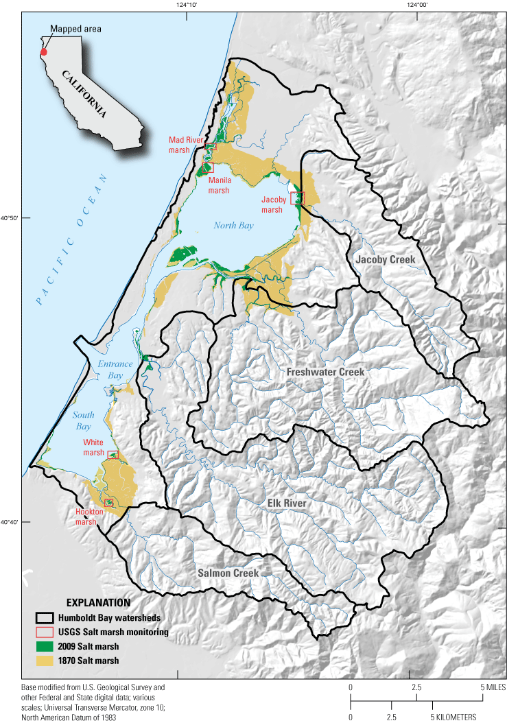
Location of Humboldt Bay, California, study area showing the three subembayments (North Bay, Entrance Bay, South Bay) and the spatial extent of salt marshes in 1870 (Laird and others, 2007) and 2009 (Schlosser and Eicher, 2012). Red bounding boxes delineate the location of five study marshes (see fig. 2 for detailed maps of the study marshes). Abbreviation: U.S. Geological Survey.
Monitoring water quality (temperature, specific conductance, salinity, turbidity, and suspended-sediment concentration) is fundamental for understanding circulation, sediment dynamics, and salt marsh processes in estuaries (Geyer and MacCready, 2014). Water temperature and salinity affect water density, which influences vertical and horizontal mixing. Water temperatures and salinity also influence salt marsh vegetation presence, species composition, and productivity (Janousek and others, 2020). Turbidity, a measure of water clarity (Anderson, 2005), influences light availability and primary production (Cloern and Jassby, 2012). Ambient suspended-sediment concentration (SSC) influences the availability of inorganic sediment to support surface deposition and elevation gain in adjacent salt marshes (D’Alpaos and others, 2011; Weston, 2014; Ganju and others, 2015).
Compared to terrestrial ecosystems, coastal vegetated habitats are small in areal extent, but the carbon density per unit area is higher (Mcleod and others, 2011). These coastal carbon sinks include tidal forests, salt marshes, and eel grass meadows (Crooks and others, 2018), which are frequently referred to collectively as blue carbon ecosystems (Nellemann and others, 2009). Across California, estuarine soil carbon storage sequesters only about 0.08 percent of the statewide annual greenhouse gas emissions, but this represents about 23 percent of the statewide annual carbon dioxide (CO2) emissions (Brown, 2019).
Within the State of California, Humboldt Bay holds the second largest area of salt marsh, making the bay a primary contributor to the blue carbon stock. These marshes provide soil-carbon storage and greenhouse gas mitigation (Brown, 2019) and shoreline protection through wave attenuation and shoreline stabilization (Shepard and others, 2011; Leonardi and others, 2016; Nicholls, 2018). Monitoring of marsh accretion processes and soil carbon storage in Humboldt Bay provides fundamental datasets for assessing coastal resiliency to climate change and determining blue carbon stocks.
Located within the intertidal zone, salt marshes are transitional landforms at the interface between marine and terrestrial environments. In this narrow coastal zone, a dynamic balance exists between sea-level, hydrodynamics, sediment supply, and plant communities (Thom, 1992; Callaway and others, 1996; Cahoon, 1997; Morris and others, 2002; Cahoon and others, 2021). This dynamic balance influences a salt marsh’s ability to trap and stabilize sediment from the surrounding environment and the availability of sediment needed to support vertical accretion.
Salt marshes build vertically and horizontally through above and below ground processes, which include internal organic production and surface accumulation of organic and inorganic material from external sources (Cahoon and others, 2006). The combined effect of these processes can result in marsh expansion through vertical accretion and horizontal progradation. Conversely, marsh loss can occur if edge erosion is ongoing or if accretion rates are lower than local rates of sea-level rise (SLR). If space is available and barriers do not exist, upslope transgression or migration of the marsh can occur, which can mitigate edge erosion and marsh loss (Kirwan and others, 2010; D’Alpaos and others, 2011; Thorne and others, 2018). Recent modeling and field studies indicate that sediment-rich salt marshes are less vulnerable to edge erosion and other impacts related to SLR, whereas sediment-limited salt marshes are more vulnerable (Patrick and DeLaune, 1990; Thom, 1992; Stralberg and others, 2011; Thorne and others, 2016).
The U.S. Geological Survey (USGS) Humboldt Bay Water-Quality and Salt Marsh Monitoring Project was designed to gain a comprehensive understanding of water-quality conditions, salt marsh accretion processes, marsh edge erosion, and soil carbon storage. From 2016 to 2019, specific conductance, temperature, salinity, and turbidity were measured in 2 tidal slough channels, SSC was calculated (using turbidity as an SSC surrogate), and marsh accretion processes (duration of flooding of the marsh surface, surface deposition, elevation change, edge erosion, soil carbon storage) were measured at 10 sites distributed across 5 study marshes. From 2010 to 2019, marsh edge erosion was estimated and the effect on blue carbon storage was assessed in four study marshes.
Objectives
The data-collection activities summarized in this report were completed by the U.S. Geological Survey (USGS) in cooperation with the California State Coastal Conservancy, the Humboldt Bay National Wildlife Refuge, and the California Department of Fish and Wildlife. The objectives of the USGS Humboldt Bay Water-Quality and Salt Marsh Monitoring Project were to (1) collect water-quality and salt marsh monitoring data; (2) make these data publicly available; (3) provide an improved understanding of water-quality conditions, marsh accretion processes, and soil-carbon storage; and (4) provide fundamental datasets needed to inform management of blue carbon stocks and assess marsh vulnerability to edge erosion and SLR. These datasets will support SLR adaptation planning and will help resource managers develop and implement sediment-based strategies (salt marsh restoration, regional sediment management, and beneficial reuse of dredged material) to build coastal resiliency to climate change.
Purpose and Scope
This report summarizes data-collection activities associated with the USGS Humboldt Bay Water-Quality and Salt Marsh Monitoring Project during water years 2016–19 and a marsh edge erosion analysis that spanned from 2010 to 2019. Note that a water year (WY) begins on October 1 of the previous calendar year and ends on September 30 of the named water year. The scope of this report includes a description of the study area, monitoring methods, summaries of the monitoring data, and a discussion of study results in the context of SLR and sediment supply. Readers are referred to previous USGS publications for additional details about related studies (Takekawa and others, 2013; Thorne and others, 2016; Curtis and others, 2019, 2021).
Study Area
Humboldt Bay (fig. 1) is located along the north coast of California. This region has a Mediterranean climate with distinct cool-dry summers and mild-wet winters. The average annual precipitation is 1,590 millimeters per year (mm/yr), of which only 3 percent falls between June and September. The local hydrology is characterized by extremes. Runoff is generated by heavy precipitation events, referred to as atmospheric rivers (Dettinger and others, 2011), which produce peak flows and high-yield watersheds deliver copious amounts of fine sediment (Curtis and others, 2021).
Humboldt Bay consists of three subembayments (North Bay, Entrance Bay, and South Bay) and is characterized by limited freshwater inputs during most of the year. The subembayments are connected by navigation channels, and an entrance channel connects the bay to the Pacific Ocean. The bay has mixed-semidiurnal tides. The mean tide level (MTL) is 1.13 meters (m; referenced to Mean Lower Low Water [MLLW]) and the mean diurnal range, estimated as the difference between MLLW and mean higher-high water (MHHW), is 2.09 m (North Spit, National Oceanic and Atmospheric Agency station 9418767; National Oceanic and Atmospheric Administration, 2022b; https://tidesandcurrents.noaa.gov/datums.html?id=9418767). Tidal exchange is approximately 114 million cubic meters per day (m3/d; Northern Hydrology & Engineering, 2015). The tidal prism, defined as the volume of tidally exchanged water, is quite large in comparison to the mean annual freshwater discharge, which is approximately 0.631 million cubic meters per year (m3/yr; Curtis and others, 2021). The large tidal exchange and relatively smaller freshwater inflows result in tidally dominated circulation.
Humboldt Bay is relatively shallow, with 70 percent of the benthic habitat comprised of tidal mudflats (Schlosser and Eicher, 2012). The water surface area is approximately 65 square kilometers (km2) at high tide and 21 km2 at low tide. At MLLW, 39 km2 of mudflats are exposed. The volume of the three subembayments is large in comparison to the tidal channels, and the morphology of the bay influences flushing rates. Approximately 41 percent of the volume of the bay is replaced during each tide cycle, and full tidal exchange can take 4 to 21 days (Schlosser and Eicher, 2012). North Bay is deeper than South Bay, and the contributions to the tidal prism are about 50 percent and 30 percent, respectively (Northern Hydrology & Engineering, 2015).
The conceptual sediment budget for Humboldt Bay includes fine-sediment (less than 63 micrometers [µm]) delivery from local watersheds and regional oceanic sources (Barnhart and others, 1992; Curtis and others, 2021). The steep mountain watersheds that discharge fluvial sediment to the bay have very high sediment yields due to regional tectonics, erodible lithology, climate, and land-use history (Brown and Ritter, 1971; Kelsey, 1980; Leithold and others, 2005; Milliman and Farnsworth, 2011; Klein and others, 2012; Warrick and others, 2013).
The primary local watersheds that deliver freshwater and fluvial sediment directly to the bay include Jacoby Creek, Freshwater Creek, Elk River, and Salmon Creek (fig. 1). Curtis and others (2021) computed a mean annual estimate of fine-grained (less than 63 µm) inorganic-sediment (herein, fine-sediment) delivery from each of the four contributing watersheds. The mean annual delivery of fine-sediment from these watersheds, computed for a baseline period spanning WY 1980 to WY 2010, was approximately 0.06±0.02 million metric tons per year, with the reported uncertainty computed using the root mean squared errors associated with statistical sediment-transport models. Jacoby Creek and Freshwater Creek flow into North Bay, and their relative contributions to fine-sediment delivery are 5 percent and 12 percent, respectively. Elk River flows into Entrance Bay, Salmon Creek flows into South Bay, and their relative contributions to fine-sediment delivery are 35 percent and 48 percent, respectively.
In Humboldt Bay, local rates of SLR, also referred to as relative SLR (Rovere and others, 2016), include the combined effect of global SLR and vertical land motion caused by tectonic subsidence (Clarke and Carver, 1992; Valentine and others, 2012). Tectonic subsidence exacerbates rates of local SLR, resulting in the highest observed rate of SLR for tide gages located along the U.S. western coastline (https://tidesandcurrents.noaa.gov/sltrends/). The trend in relative SLR for the North Spit, California, tide gage, calculated using monthly mean sea-level data from 1977 to 2021, is 4.9±0.8 mm/yr (National Oceanic and Atmospheric Administration, 2022a; https://tidesandcurrents.noaa.gov/sltrends/sltrends_station.shtml?id=9418767). This trend in relative SLR is higher than published regional averages for the State of California (Russell and Griggs, 2012) and the rest of the Pacific Northwest (Montillet and others, 2018). Tectonic subsidence varies across the bay, and recent estimates of relative SLR that consider this variability are 3.11 mm/yr for North Bay and 5.56 mm/yr for South Bay (Northern Hydrology & Engineering, 2015).
The sheltering effect of barrier spits protects the interior of the bay from wave exposure. Through time, this sheltering effect allowed the formation of salt marshes in low-energy environments. The present distribution of salt marsh provides multiple ecosystem services that include carbon sequestration and greenhouse gas mitigation, natural shoreline protection, habitat for resident and migratory birds, and habitat for rare marsh-dependent plants, such as Humboldt Bay owl’s clover (Castilleja ambigua spp. humboldtiensis), Pt. Reyes bird’s-beak (Chloropyron maritimum ssp. palustre), and western sandspurry (Spergularia canadensis var. occidentalis).
Methods
This study included (1) continuous water-quality monitoring in two tidal channels to determine water-quality conditions, (2) continuous monitoring of water levels and quarterly monitoring of surface deposition and elevation change in five study marshes, (3) sediment-core collection in five study marshes to determine soil-carbon storage in edge environments, and (4) analysis of repeat aerial imagery and elevation surveys to determine rates of marsh edge erosion and impacts to blue carbon storage in four study marshes. A level of significance (α) of 0.05 was used for all statistical analyses presented in this report.
Water-Quality Monitoring
Water-Quality Conditions
In 2016, two water-quality stations (table 1) were established in Mad River Slough (USGS station 405219124085601) and Hookton Slough (USGS station 404038124131801; U.S. Geological Survey, 2021), which are the primary tidal channels that convey water and suspended sediment into two adjacent study marshes (fig. 2). Continuous observations of water temperature (reported in degrees Celsius [°C]), specific conductance (reported in microsiemens per centimeter [μS/cm] at 25 °C), salinity (reported in practical salinity units [PSU]), and turbidity (reported in formazin nephelometric units [FNU]) were collected every 15-minutes using multiparameter sondes (EXO2, YSI Inc., Yellow Springs, Ohio, USA). The sondes were equipped with a combined temperature and specific conductance sensor and an optical turbidity sensor. Optical side-scattering turbidity sensors, which measure the amount of light reflected at a 90-degree angle, were used because they are less sensitive to changes in particle size than optical backscatter sensors (Druine and others, 2018).
Table 1.
Parameters measured at two U.S. Geological Survey (USGS) water-quality and water-level monitoring stations in Humboldt Bay, California, during water years 2016–19 (U.S. Geological Survey, 2021).[mm/dd/yyyy, month/day/year; USGS, U.S. Geological Survey; FNU, formazin nephelometric units; µs/cm, microsiemens per centimeter; °C, degrees Celsius; m, meter]
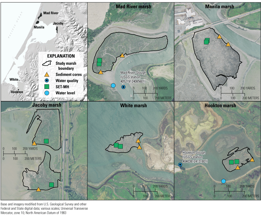
Depiction of the U.S. Geological Survey (USGS) water-quality and salt marsh monitoring network in Humboldt Bay, California, showing the location of five study marsh sites, surface elevation tables (SET) and marker horizons (MH), two water-level loggers, two water-quality stations, and locations of sediment cores (U.S. Geological Survey, 2021).
Sondes equipped with a central wiper were mounted to a moored oyster raft in Mad River Slough and a non-motorized floating boat ramp in Hookton Slough. The sondes were suspended from a stainless-steel cable and deployed within a perforated galvanized steel pipe at a fixed water depth (1-meter below the water surface). The sondes collected a 40-second burst of data, which was averaged and recorded for each 15-minute timestamp. Biological activity and growth, referred to as biofouling, can interfere with sensor readings. To minimize biofouling, sensors were wrapped in anti-fouling copper tape. The sondes were programmed to wipe the optical turbidity sensors before every measurement and sensors were cleaned monthly.
Water-quality records were collected, archived, analyzed, and approved following standard USGS guidelines (Wagner and others, 2006). During quarterly visits, fouling checks were performed, and sensor performance was evaluated. Fouling checks were performed by comparing sensor output before and after each cleaning. The fouling checks were used to quantify a biofouling correction for post-processing. Sensor performance was checked by comparing sensor output measured in calibration solutions with known values using solution standards that bracketed the range of measured water-quality conditions. The calibration checks were used to identify sensor drift, calibration errors, and sensor malfunction, and to quantify drift corrections for post-processing. The sensor output for temperature was checked using a National Institute of Standards and Technology (NIST) traceable thermistor. The sensor output for specific conductance and turbidity was checked against and, if needed, calibrated to calibration solutions with known values. During post-processing, fouling and drift corrections were applied to the time-series records as needed.
The 15-minute records for five water-quality parameters (temperature, specific conductance, salinity, turbidity, and SSC) were published separately on the USGS NWIS data portal (U.S. Geological Survey, 2021; https://waterdata.usgs.gov/ca/nwis/uv). Parametric and non-parametric tests, with site as the factor, were used to compare the data distributions and to check for statistically significant differences between sites. Equal variance was checked using Levene’s test, normality was checked using the Kolmogorov-Smirnov test, and the normal and chi-square approximations for the Wilcoxon test statistic were used to test for statistical significance (p<0.05; Helsel and others, 2020).
Discrete Water Samples
During quarterly site visits, single-point water samples were collected at a fixed depth of 1-meter below the instantaneous water level using a Van Dorn sampler (Holmes and others, 2001). Samples at the Mad River and Hookton water-quality stations were collected alongside the sensors, throughout a complete rising and falling tidal cycle, and typically at 1.5-hour intervals. The sampler was lowered to the depth of the sensor and remotely triggered to collect a water sample.
At each water-quality station, the depth and width of the flooded channel varied with tidal conditions. At the Mad River Slough station (fig. 3A), the point samples were collected near the sonde, which was mounted to a floating oyster raft moored in the center of the tidal channel. During sample collection, tidal channel depth varied from 3.5 to 10 m, and width varied from 55 to 150 m. At the Hookton Slough station (fig. 3B), point samples were collected near the sonde, which was mounted on a floating non-motorized boat ramp on the left bank of the channel. During sample collection, tidal channel dimensions ranged from 0.75 to 4 m deep and 25 to 55 m wide.
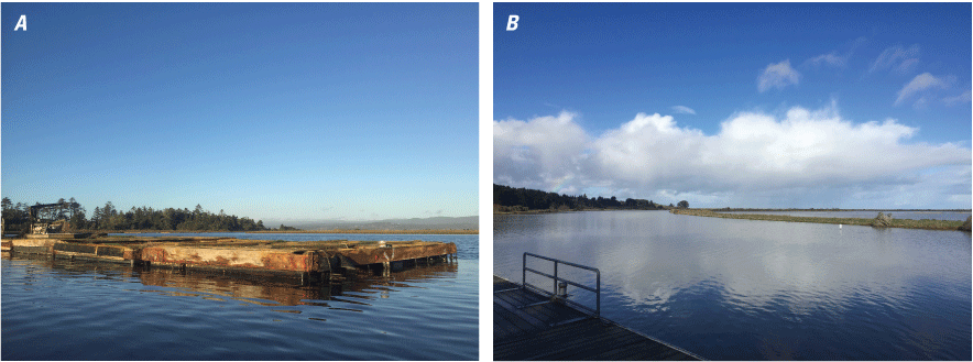
U.S. Geological Survey (USGS) water-quality monitoring stations (U.S. Geological Survey, 2021) deployed at A, Mad River Slough (U.S. Geological Survey station 405219124085601) and B, Hookton Slough (U.S. Geological Survey station 404038124131801).
Water samples were stored in brown high-density polyethylene (HDPE) bottles, kept cool, and shipped to the USGS Cascade Volcanic Observatory sediment laboratory (Vancouver, Washington) for SSC analysis. The SSCs were determined by filtration or evaporation methods following standard test methods (American Society for Testing and Materials, 2002), with the method dependent upon total sample mass. Suspended sediment included all particles in the sample that did not pass through a 0.45-µm membrane filter. The evaporation method was used to measure the mass of the finest sediment (this method requires a few days to a few weeks for sediment to settle), and a correction factor was applied if the dissolved-solids concentration exceeded 10 percent of the total sediment concentration. The filtration method was used on samples containing clay concentrations of less than about 200 parts per million (ppm). The filtrate was rinsed with de-ionized water to remove salts, and a correction factor for dissolved solids was not required. The SSC samples were dried at 103 °C and weighed. Sample mass was determined and divided by the original volume of water in the sample to obtain SSC, which is reported in milligrams per liter (mg/L). A complete inventory of water-quality samples for each water-quality station is available through the USGS NWIS (U.S. Geological Survey, 2021; https://nwis.waterdata.usgs.gov/usa/nwis/qwdata).
Surrogate Regression Models
Turbidity, an optical property of water (Anderson, 2005), was used as a surrogate measurement for computing a continuous time series of SSC (Downing, 2006; Rasmussen and others, 2009). Computation of SSC required the development of two surrogate regression models. Detailed information about the regression models used to compute SSC from the turbidity, along with an in-depth description of the regression analysis, were published in Curtis (2021a, b)15.
A description of the surrogate regression models and the goodness-of-fit statistics are provided herein for completeness. Base-10 logarithm (log10) transformation improved the goodness-of-fit for the Hookton Slough model (eq. 1; Curtis, 2021a), and the bias correction factor (BCF) for addressing retransformation bias is reported. The Mad River Slough model is a simple linear model (eq. 2; Curtis, 2021b). The mean squared percent error (MSPE) for the surrogate models was similar. The slope and the coefficient of determination (R2) for the Mad River model were low due to the small range of values in the turbidity and SSC datasets. The low R2 value indicates high variability within this small range of input values. Although the Mad River regression model is statistically significant (p<0.0001), turbidity appears to be a poor predictor variable at this site.
whereSalt Marsh Monitoring
Marsh monitoring (duration of flooding of the marsh surface, surface deposition, elevation change, edge erosion, and soil-carbon storage) was completed in five study marshes (table 2) distributed throughout Humboldt Bay (fig. 2). Four of the study marshes (Mad River, Jacoby, White, and Hookton) are managed by the U.S. Fish and Wildlife Service—Humboldt Bay National Wildlife Refuge. Manila marsh is managed by the California Department of Fish and Wildlife.
Table 2.
Descriptions and attribute information for five salt marshes located in Humboldt Bay, California.[Elevation estimates are from Curtis and others (2019). Relative sea-level rise (SLR) estimates are from Northern Hydrology & Engineering (2015). Abbreviations: km2, square kilometer; NAVD 88, North American Vertical Datum of 1988; m, meter; mm/yr, millimeter per year]
Three of the study marshes (Mad River, Manila, and Jacoby) are located in North Bay, and two study marshes (White and Hookton) are located in South Bay (fig. 1). Mad River marsh is a high elevation island (about 83 percent of the area above MHHW) located within Mad River Slough. Manila marsh is a low elevation marsh (about 10 percent of the area above MHHW) located at the bay-slough interface. Jacoby marsh is a high elevation deltaic marsh (about 81 percent of the marsh area above MHHW) located at the mouth of Jacoby Creek. White marsh is a low-elevation island marsh (about 1 percent of the marsh area above MHHW) located at the bay-slough interface. Hookton marsh is a low-elevation island marsh (about 8 percent of the area is above MHHW) located within Hookton Slough.
Water Levels and Tidal Datums
Water-level and barometric-pressure data loggers were deployed in the tidal channels of two study marshes (fig. 2; Mad River and Hookton). Initially, Onset-Hobo sensors (Model U-20-001-01-Ti, Onset Computer Corp., Bourne, Massachusetts, USA; 0.5-centimeter [cm] accuracy) were deployed (table 1). The Hobo sensors were replaced by higher accuracy Solinst-Edge LT sensors (Model 3001, Solinst Canada Ltd., Georgetown, Ontario, Canada; 0.3-cm accuracy). The loggers were programmed to collect measurements (absolute pressure, barometric pressure, air temperature, and water temperature) on a 6-minute timestep. Sensors were mounted on t-posts, close to the channel edge, and as low in the tidal prism as possible while still maintaining access to the sensors at low tide. Following deployment, the sensor locations were surveyed with Real-Time Kinematic GNSS (RTK-GNSS; Leica GS-15, Leica Geosystems, Norcross, Georgia, USA; 2.0-cm accuracy). During quarterly site visits, the loggers were downloaded, cleaned, and resurveyed to record any changes in vertical position.
The water-level and barometric-pressure loggers recorded absolute pressure and barometric pressure using height units (m) and a pre-programmed density of 1,000 kilograms per cubic meter (kg/m3). The measured data were post-processed in the R statistical environment (R Core Team, 2019) Absolute pressure and barometric pressure were converted to pressure units of kilopascals (kPa), and water pressure was computed by subtracting the barometric pressure from the absolute pressure. The resulting barometric-compensated water pressure was then converted back to a water-level height relative to the sensor using equation 3:
whereP
is the atmospheric-corrected water pressure (kPa),
ρ
is saltwater density (1,025 kg/m3), and
k
is a unit conversion constant of 9.80665.
Data were visually inspected for anomalous readings and sensor failure indications. Continuous 6-minute records (air temperature, water temperature, sensor elevation, barometric pressure, and water level) were published in Curtis and others (2022).
The water levels for Mad River and Hookton marshes were used to calculate site-specific tidal datums, develop local hydrographs, determine the duration of flooding of the marsh surface, and assess water elevations during extreme events. Two local tidal datums mean high water (MHW) and MHHW were estimated for the two marshes using standard guidelines (Evans and others, 2003). The water-level loggers were positioned relatively high in the intertidal zone and did not capture the low water levels necessary to compute mean low water (MLW) or MLLW. The mean tide level (MTL) for each site was computed using the National Oceanic and Atmospheric Administration (NOAA) VDATUM 3.4 software (Xu and others, 2010).
Surface Deposition and Elevation Change
Deep rod surface elevation tables (SETs) and feldspar marker horizon (MH) plots (fig. 2) were installed in the five study marshes to quantify the relative contributions of surface and subsurface processes to accretion and elevation change. Steel rods were driven to the point of refusal (32–60 m), establishing a benchmark from which to measure changes in surfacing elevation. The SET measurements quantify surface-elevation change, and the MH measurements quantify surface deposition upon a feldspar layer applied on the marsh surface. Surface deposition is defined as the vertical buildup of mineral and organic sediment on the marsh surface, and elevation change is defined as a change in the total height of the marsh surface due to the net effect of below and above ground processes (fig. 4). Subsidence is divided into shallow and deep components. Shallow subsidence is the elevation loss measured from the bottom of the deep rod to the MH layer and is the result of organic decomposition and soil consolidation processes (fig. 4). Deep subsidence refers to any elevation change below the deep rod and is not measured by the SET; this movement is typically tectonic in nature.
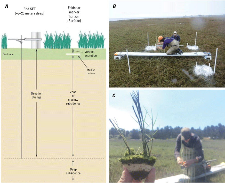
A, Conceptual diagram showing how the elevation of the marsh surface is measured by a marker horizon (MH) and a surface elevation table (SET) to assess surface and subsurface processes, respectively (Cahoon and others, 2002); B, photograph showing U.S. Geological Survey technicians reading a SET; and C, photograph showing the feldspar MH.
At each of the five study marshes, two representative monitoring locations were selected for installing SET-MHs after considering surface elevations, vegetation composition, and distance from tidal sources. At each monitoring location, one SET was paired with three MHs, following standard guidelines (Cahoon and others, 2002; Webb and others, 2013; Lynch and others, 2015). Thus, a total of two SETs and 6 MHs were installed in each study marsh.
The SET-MHs were measured during quarterly site visits. Surface deposition was measuring for each MH by removing a small plug of soil using a soil knife, measuring the depth of surface deposition above the feldspar layer on four sides, and replacing the plug. This method yielded four measurements of surface deposition per MH per year. Elevation change was measured by attaching the SET instrument to a collar installed on top of a local benchmark, in this case, the top of the deep rod (fig. 4). During each measurement, 9 pins were lowered to the surface in four 90-degree cardinal directions yielding 36 observations of elevation change per SET.
Quarterly SET-MH measurements were published in Curtis and others (2022). SETs at Mad River and Manila were installed in 2013. Because baseline measurements for these two sites were collected before the monitoring period described in this report, negative surface-deposition measurements at the MH were possible. One-way analysis of variance (ANOVA), with a post-hoc Tukey Honest Significant Difference test, was used to compare rates of elevation change and surface deposition across the study marshes and to compare pair-wise site combinations (Helsel and others, 2020).
Soil Carbon Storage
A total of 10 sediment cores were collected within 2 m of the marsh edge in the 5 study marshes to characterize soil carbon storage where edge erosion may occur (fig. 2). Two sediment cores were collected in each marsh using an Eijkelkamp peat sampler (52-mm diameter), which was pounded into the sediments with a heavy plastic mallet. This method produces little to no compaction because once inserted, the core is rotated 180 degrees, and a sample is collected adjacent to where it was driven into the ground. Cores approximately 1-meter in depth were collected at all sites except the southern-most cores collected at Jacoby marsh, where a sandy substrate limited the core depth to 50 cm. The cores were sectioned at 10-cm intervals in the field and placed in labeled, pre-weighed metal tins. The 10-cm core sections were transported on ice to the USGS soils laboratory in Sacramento, California, and were then refrigerated. Following methods described in Drexler and others (2009), core sections were weighed, dried at 50 °C for 72 hours, and then re-weighed. Bulk density was determined by dividing the dry weight by the core volume for each 10-cm section of core.
Dried and weighed core sections were subsequently analyzed for percent organic carbon at the University of California, Davis Analytical Laboratory, using acid fumigation and dynamic flash combustion following methods described in Harris and others (2001) and the Association of Official Analytical Chemists (1997) Official Method 972.43. The lab detection limit for percent organic carbon was 0.02 percent. Replicate samples were analyzed every 10 samples to check for instrument drift. Carbon density was determined for each core section by multiplying bulk density by percent organic carbon.
ANOVA, with site as the factor, was used to compare mean core values for bulk density, percent organic carbon, and carbon density across sites. Only carbon density required a Log10 transformation to meet ANOVA assumptions. Homogeneity of variances was checked using Levene’s test, and normality was checked using the Shapiro-Wilk test (Helsel and others, 2020). Sediment-core data were published in Curtis and others (2022).
Marsh Edge Erosion
Horizontal retreat in four of the five study marshes was assessed by completing change-detection analysis to determine edge erosion using available 4-band orthoimagery and LiDAR-derived elevation data. Two LiDAR datasets, acquired during low tide conditions in 2010 (2009–11 California Coastal Conservancy Coastal Lidar Project; Office for Coastal Management, 2021a) and 2019 (2019 Lidar: Eureka, California, OCM Partners, 2021), were downloaded as point clouds (.laz) from the NOAA Digital Coast viewer (https://coast.noaa.gov/dataviewer). The 2010 LiDAR has a point density of 1 point per square meter (pt/m2), while the 2019 LiDAR has a density of at least 17 pt/m2. The 2010 orthoimagery (Office for Coastal Management, 2021b), with a resolution of 0.3 m, was collected at the same time as the LiDAR. The 2019 orthoimagery (Office for Coastal Management, 2021c), with a resolution of 0.04 m, was collected at the same time as the LiDAR, but does not cover Hookton marsh. For this reason, marsh edge erosion was only assessed at four study marshes.
Before performing the change detection analysis to assess edge erosion, the 2019 imagery was resampled to 0.3 m using bilinear interpolation. Triangular irregular networks were used to generate digital elevation models (DEMs) for the 2010- and 2019-point clouds at 0.3-m resolution to match the orthoimagery (lidR package in R, grid_terrain function; Roussel and Auty, 2020). The LiDAR and orthoimagery were then visually inspected for co-registration issues, but no changes in georeferencing were necessary.
The first step in the change detection analysis was to calculate a normalized difference vegetation index (NDVI) for each orthoimage using the red and near-infrared bands. The NDVI rasters were then clipped with a boundary that surrounded each study marsh and included marsh and mudflat habitats. An unsupervised classification was implemented in ArcPro v2.6.1 (https://support.esri.com/en/Products/Desktop/arcgis-desktop/arcgis-pro/2-6) using the Iterative Self-Organizing (ISO) cluster tool. The cluster analysis was run, with a maximum of 30 classes and a minimum of 200 pixels per class, using the NDVI and the DEM for each year. The resulting classes were then assigned to a vegetated or unvegetated class on the basis of visual comparison with the orthoimagery.
Boundaries for assessing marsh edge erosion for each study marsh were generated by buffering polygons that depict the areal extents of salt marshes in 2009 (Schlosser and Eicher, 2012). The buffer size was interactively determined to ensure it surrounded the entire area of interest. At Jacoby marsh, which showed the most change, the buffer (50 m total) extended 40 m toward the marsh interior and 10 m toward the intertidal zone, whereas at all other sites (20 m total), the buffer extended 10 m in both directions. The classified 2010 and 2019 rasters were clipped to the buffered area. The vegetated and unvegetated areas within the buffered boundary for each study marsh were summed, and marsh edge erosion was determined by subtracting the total unvegetated area in 2010 from the total unvegetated area in 2019.
To estimate uncertainty caused by co-registration issues and mismatch in LiDAR point density, the resulting marsh edge erosion raster was contracted and expanded by one pixel to create a 3-pixel uncertainty buffer for analysis. This method provided a very conservative estimate of edge change where only areas at least three pixels (0.9 m) wide were classified as eroded. The average and standard deviation of areas experiencing edge erosion area were calculated using the initial and conservative estimates.
Results and Discussion
Monitoring results captured spatial and temporal variations in water-quality conditions and marsh processes. Graphical and tabular summaries of monitoring data, marsh edge erosion, and the impacts of edge erosion on blue carbon storage are presented.
Water-Quality Conditions
A series of plots showing temporal variations in temperature, salinity (computed from temperature-compensated specific conductance; Wagner and others, 2006), turbidity, and SSC (computed using turbidity as a surrogate) are presented for the Mad River Slough (fig. 5) station (405219124085601; U.S. Geological Survey, 2021) and the Hookton Slough (fig. 6) station (404038124131801; U.S. Geological Survey, 2021). Sensor failure resulted in large data gaps in the salinity record in 2018 and 2019. In comparison, percent missing values for the period of record for the turbidity sensors were 0.1 percent at the Hookton Slough station and 1.1 percent at the Mad River Slough station. The horizontal and vertical scales in figures 5 and 6 are the same to aid with visual comparisons between the two sites.
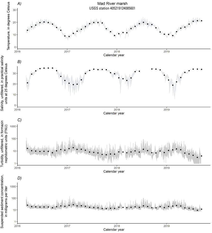
Summary of water-quality monitoring during 2016–19 for A, temperature; B, salinity; C, turbidity; and D, suspended-sediment concentration for Mad River Slough (USGS station 405219124085601; U.S. Geological Survey, 2021). Gray lines represent continuous measurements and black dots are the monthly average.
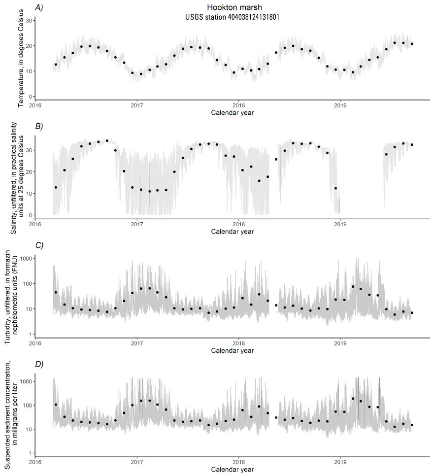
Summary of water-quality monitoring during 2016–19 for A, temperature; B, salinity; C, turbidity; and D, suspended-sediment concentration for Hookton Slough (USGS station 404038124131801; U.S. Geological Survey, 2021). Gray lines represent continuous measurements and black dots are the monthly average.
Statistical tests used to compare the data distributions for the five water-quality parameters indicated that water-quality conditions were spatially and temporally variable. The Kolmogorov-Smirnov tests indicated non-normal distributions for the five water-quality parameters, and the normal and chi-square approximations for the Wilcoxon test statistic indicated statistically significant differences (p<0.0001) between the two stations for all five water-quality parameters.
Water temperatures (table 3) and salinities (table 4) were higher at the Mad River Slough station indicating lower freshwater inputs and tidal exchange rates. The minimum salinity at the Hookton Slough station was lower (near zero) than at the Mad River Slough station (6 PSU), and the timing of the increase in seasonal freshwater discharge at Hookton corresponded to higher SSCs (fig. 6). Measured values of turbidity (table 5) and computed values of SSC (table 6) were higher at the Hookton Slough station, indicating a larger supply of mobile sediment and greater availability of suspended sediment to support marsh surface deposition and elevation gain. The mean SSC (table 6) at the Hookton Slough station was almost 3 times higher than the estimate for the Mad River Slough station, but the median estimates for the two stations were similar. On the basis of the 90-percent confidence intervals, the mean SSC at the Mad River Slough station was between 11 and 24.6 mg/L, and the mean SSC at the Hookton Slough station was between 28.5 and 72.9 mg/L. Measures of statistical variance (standard deviation, coefficient of variation, and the range of values) for turbidity and SSC were much larger for the Hookton Slough station, indicating that event-driven sediment transport occurs more frequently at this site.
Table 3.
Statistical summary of water temperature observations for two water-quality monitoring stations in Humboldt Bay, California, during water years 2016–19 (U.S. Geological Survey, 2021).[USGS, U.S. Geological Survey; temp, temperature; °C, degrees Celsius; SD, standard deviation; CV, coefficient of variation; %, percentage; Min, minimum; Max, maximum]
Table 4.
Statistical summary of salinity observations for two water-quality monitoring stations in Humboldt Bay, California, during water years 2016–19 (U.S. Geological Survey, 2021).[USGS, U.S. Geological Survey; PSU, practical salinity units at 25 degrees Celsius; SD, standard deviation; CV, coefficient of variation; %, percentage; Min, minimum; Max, maximum]
Table 5.
Statistical summary of turbidity observations for two water-quality monitoring stations in Humboldt Bay, California, during water years 2016–19 (U.S. Geological Survey, 2021).[USGS, U.S. Geological Survey; SD, standard deviation; CV, coefficient of variation; %, percentage; Min, minimum; Max, maximum; FNU, formazin nephelometric units; >, greater than]
Table 6.
Statistical summary of suspended-sediment concentrations computed from continuous turbidity records for two water-quality monitoring stations in Humboldt Bay, California during water years 2016–19 (U.S. Geological Survey, 2021).[USGS, U.S. Geological Survey; SSC, suspended-sediment concentration; ±, plus or minus; %, percentage; CI, confidence interval; mg/L, milligrams per liter; SD, standard deviation; CV, coefficient of variation; Min, minimum; Max, maximum]
Duration of Flooding of the Marsh Surface
Daily and monthly water-level hydrographs for Mad River marsh and Hookton marsh are shown on figures 7 and 8. Although the water-level loggers did not capture the lower parts of the tidal signal because of their location within the tidal frame, water-level monitoring indicated Mad River marsh had a slightly higher MHHW than Hookton marsh. For both study marshes, the estimates for MHHW and MHW (table 7) were slightly greater than estimates reported for the nearby NOAA station (North Spit NOAA station 9418767; https://tidesandcurrents.noaa.gov/datums.html?id=9418767), and estimates for MTL computed using VDATUM were slightly lower. Repeat elevation surveys indicate vertical movement in the water-level loggers was less than the instrument error of the RTK-GNSS (2 cm). Differences in the tidal datums likely reflect site-specific tidal and bathymetric conditions and variations in local estuarine hydrology.
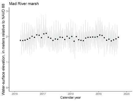
Summary of water-level monitoring (in meters) referenced to the North American Vertical Datum of 1988 (NAVD 88) for Mad River marsh from 2016 to 2019 (Curtis and others, 2022). Gray lines represent high tide levels, and black dots are monthly high tide averages.
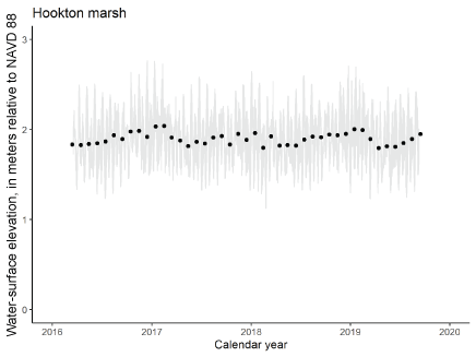
Summary of water-level monitoring (in meters) referenced to the North American Vertical Datum of 1988 (NAVD 88) for Hookton marsh from 2016 to 2019 (Curtis and others, 2022). Gray lines represent high tide levels, and black dots are monthly high tide averages.
Table 7.
Site-specific tidal datums referenced to the North American Vertical Datum of 1988 (NAVD 88, in meters) for two marshes calculated using measured water levels except as noted.[Datums for the North Spit tide gauge (NOAA 9418767) at the mouth of the bay are provided as a comparison (National Oceanic and Atmospheric Administration, 2022b). Abbreviations: m, meters; NOAA, National Oceanic and Atmospheric Administration; HOWL, highest observed water level; MHHW, mean higher high water; MHW, mean high water; MTL, mean tide level; yr, year; mo, month; —, no data]
| Site | Period of record |
HOWL | MHHW | MHW | MTL |
|---|---|---|---|---|---|
| Mad River marsh | 3 yr 6 mo | 2.88 | 2.013 | 1.796 | 0.953* |
| Hookton marsh | 3 yr 6 mo | 2.77 | 1.985 | 1.745 | 0.946* |
| North Spit (9418767) | 1983–2001 (epoch) | — | 1.987 | 1.77 | 1.025 |
Values estimated from VDATUM model (Xu and others, 2010).
Marsh Surface Deposition and Elevation Change
SET measurements quantify elevation change, and feldspar MH measurements quantify surface deposition (Cahoon and others, 2002; Lynch and others, 2015). If surface deposition is greater than the amount of elevation change, shallow subsidence (surface deposition minus elevation change) related to decomposition or compaction may be occurring. If surface deposition is equal to elevation change, deposition is likely driving elevation change, and subsurface processes are assumed to be negligible. If surface deposition is less than elevation change, shallow expansion related to swelling of soils by water storage or an increase in root volume may be occurring.
During the monitoring period, elevation changes and surface deposition were spatially and temporally variable (table 8). Across all five study salt marshes, mean annual surface deposition was 2.5±0.5 mm/yr, and the mean annual elevation change was 1.8±0.6 mm/yr. Post-hoc Tukey results from the ANOVA analysis indicated the rates of elevation change and surface deposition were significantly different (p<0.05) among all the study marsh combinations, with one exception. The post-hoc Tukey results indicated no significant differences in elevation change (p=1.0) and surface deposition (p=0.93) between Hookton and White marshes. For the South Bay marshes (Hookton and White), surface deposition rates were 1.2 times greater than elevation changes. In the North Bay marshes (Mad River, Manila, and Jacoby), surface deposition rates were 1.7 times greater than rates of elevation change (table 9). These results indicated that subsurface processes resulted in some elevation loss across the Humboldt Bay marshes during the study period (fig. 9).
Table 8.
Summary of mean annual rates of elevation change and surface deposition, reported as the mean plus or minus (±) the standard error, during the monitoring period from water year 2016 to 2019 for five study marshes located in Humboldt Bay, California (Curtis and others, 2022).[WY, water year; mm/yr, millimeters per year]
Table 9.
Cumulative changes in elevation and surface deposition and average annual rates of elevation change and surface deposition, reported as the mean plus or minus (±) the standard error, during the monitoring period from water years 2016 to 2019 for five study marshes located in Humboldt Bay, California (Curtis and others, 2022).[mm, millimeters; yr, year]
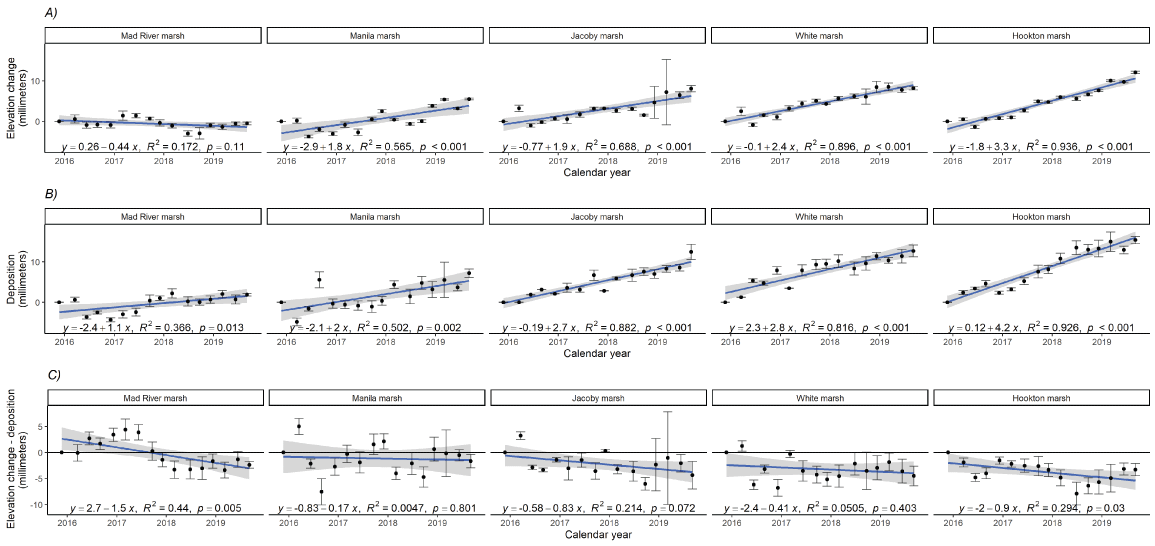
Mean values and the associated standard errors for A, elevation change; B, surface deposition; and C, the difference between elevation change and surface deposition across five study marshes in Humboldt Bay. Black points represent quarterly readings collected during the 4-year monitoring period (Curtis and others, 2022). The difference between net-elevation change and surface deposition indicates the primary driver of accretion. Negative values indicate accretion is driven by deposition, while positive values indicate that below-ground processes are dominant. The gray shading represents the 95-percent confidence interval for the linear regression.
During the monitoring period, mean annual rates of surface deposition and elevation change in the South Bay marshes were nearly twice the rates measured in the North Bay marshes (table 9). Across all five study marshes, elevation changes were lower during WY 2016 and WY 2018 and higher in WY 2017 and WY 2019 (table 8). However, surface deposition across all the South Bay sites was more consistent across water years compared to the North Bay sites (table 8). Increases in net elevation change were significantly correlated with longer flooding time in three marshes (Jacoby, Mad River and White), while surface deposition was positively correlated with the duration of surface flooding only at Jacoby marsh (fig. 10). In vegetated marshes, a longer flooding period allows more time for sediment to deposit on the marsh surface and more opportunity for salts to be flushed from the soil, potentially increasing plant productivity. Figure 9C shows decreasing trends with negative values for Mad River, Jacoby, White, and Hookton marshes, indicating accretion was driven by surface deposition at most sites during the study period.
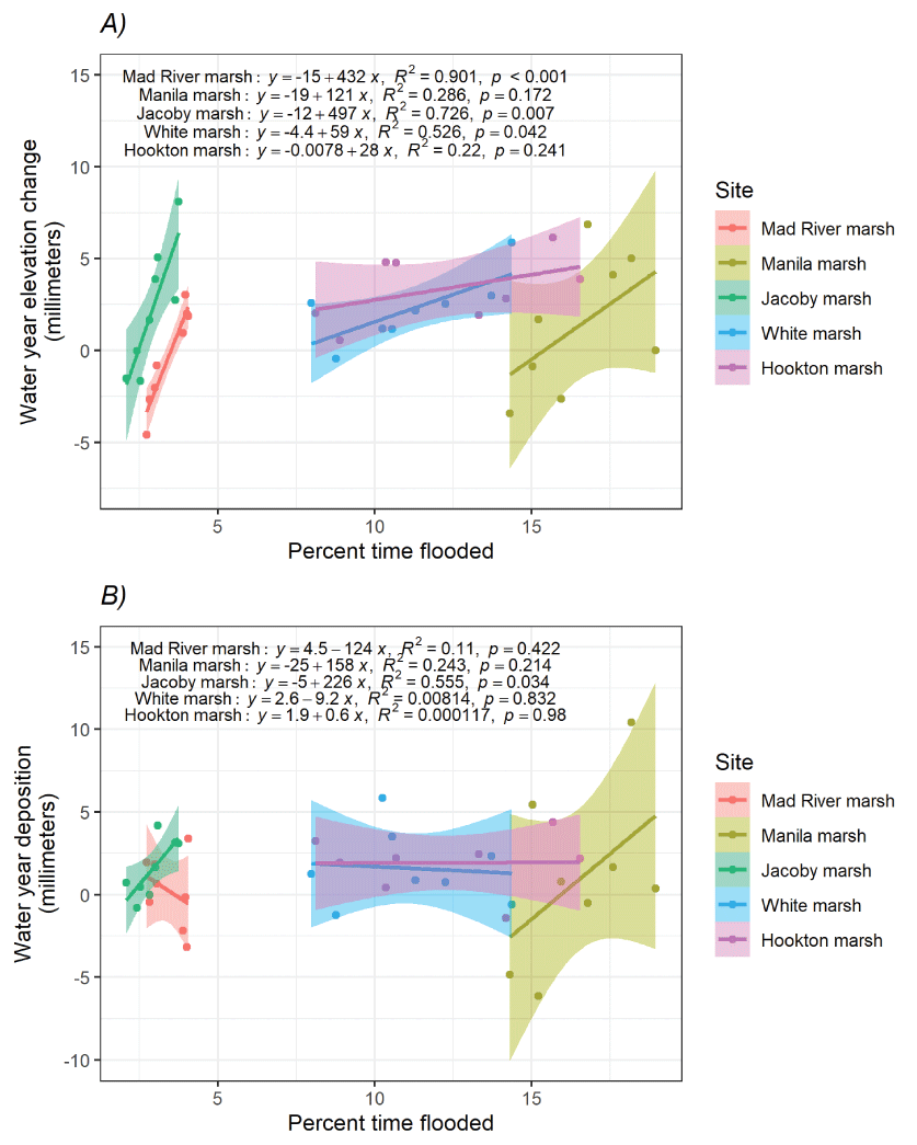
A, water year elevation change; and B, water year deposition compared to the corresponding flooding rates based on the mean elevation of the surface elevation tables at each of the five study sites (Curtis and others, 2022). Points represent annual rates of elevation change or deposition during the monitoring period from water years 2016 to 2019 for five study marshes located in Humboldt Bay, California.
These short-term results represent initial baseline measurements and should be interpreted with caution because long-term monitoring may show different trends. Continued monitoring, over decadal or longer periods to capture stochastic processes that influence SLR (fig. 11A), and wet and dry water years (fig. 11B) could help identify trajectories and magnitudes of trends throughout longer timescales.
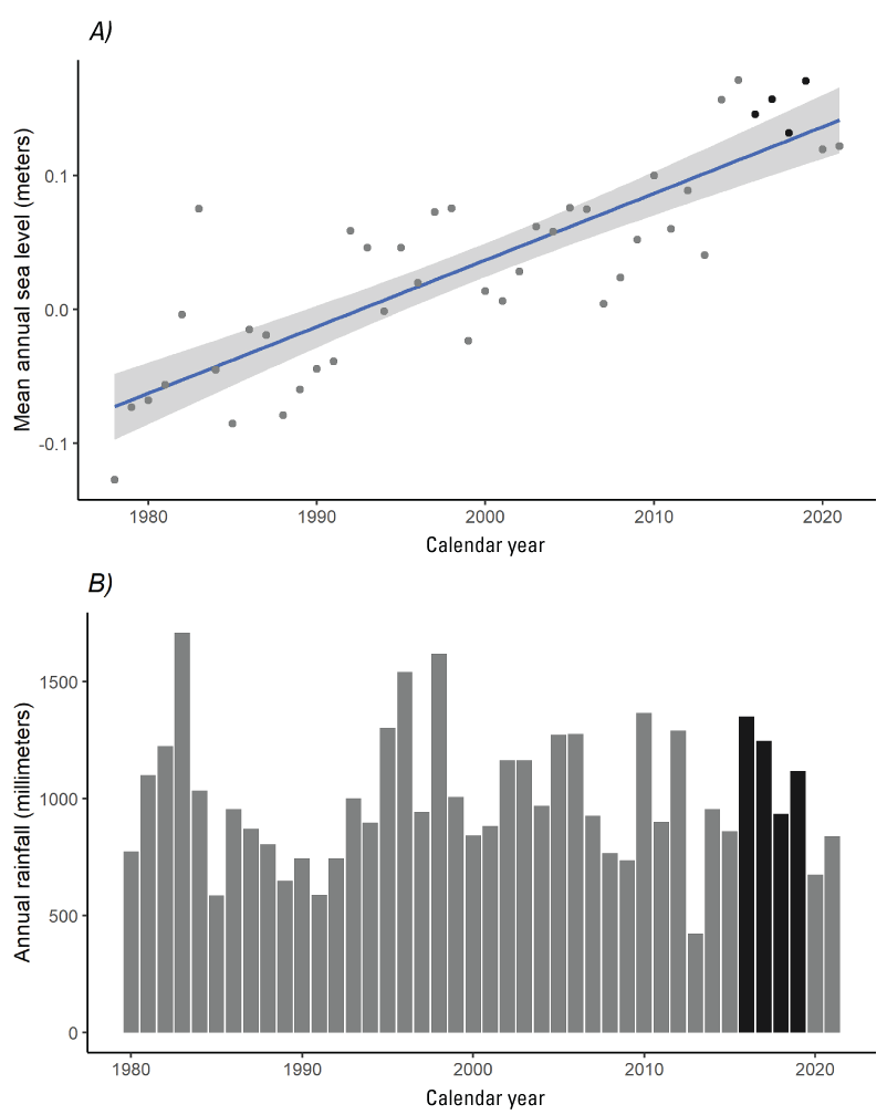
Physical data showing the representativeness of the monitoring period (black symbols) relative to recent history (gray symbols). A, mean annual sea level (NAVD 88 in meters) for the North Spit (station: 9418767; National Oceanic and Atmospheric Administration, 2022a), with gray shading shown to represent the 95-percent confidence interval along the trend line; B, annual rainfall totals (millimeters) for Eureka, California (station: GHCND: USW00024213; National Centers for Environmental Information, 2022)
Soil Carbon Storage in Five Study Marshes
Marsh cores collected in the five study marshes are similar with respect to percent organic carbon content and carbon density. One-way ANOVA results for the five marshes indicated a significant difference for bulk density measurements (one-way ANOVA, p=0.010; table 10). Post-hoc pairwise comparisons using Tukey’s Honestly Significant Difference test showed that the northern part of Jacoby marsh (p=0.006), Manila marsh (p=0.033), and Mad River marsh (p=0.047) all had statistically significantly greater bulk density than White marsh; however, bulk densities were not significantly different among any of the other sites (p>0.05). The mean bulk density for all the sediment cores collected across the five study marshes, was 0.82±0.08 grams per cubic centimeter (g/cm3) and ranged from 0.649 to 0.957 g/cm3 (fig. 12); the mean percent organic carbon was 3.8±0.9 percent and ranged from 2.29 to 5.84 percent (fig. 13). Mean percent organic carbon values were not significantly different among the five sites (one-way ANOVA, p=0.119).
Table 10.
One-way analyses of variance (ANOVAs) for bulk density, percent organic carbon, and carbon density (Curtis and others, 2022) with site as the factor.[ANOVA, analysis of variance; —, not applicable]
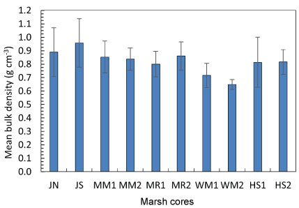
Mean soil bulk density (blue bars) in grams per cubic centimeter (g/cm3) and standard deviations (error bars) for cores collected in five study marshes in Humboldt Bay, California (Curtis and others, 2022). Core abbreviations are as follows: JN, northern part of Jacoby marsh; JS, southern part of Jacoby marsh; MM, Manila marsh; MR, Mad River marsh; WM, White marsh; and HS, Hookton marsh. The numbers 1 and 2 refer to each of the two cores collected at sites, whereas JN and JS represent the two cores collected at Jacoby Marsh.
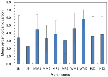
Mean percent organic carbon by weight (blue bars) and standard deviations (error bars) for cores collected in five study marshes in Humboldt Bay, California (Curtis and others, 2022). Core abbreviations are provided in figure 12.
The mean carbon density for all the sediment cores collected across the five study marshes was 0.029±0.005 grams of carbon per cubic centimeter (g C/cm3; fig. 14). This value is similar to the mean carbon density reported for the top meter of 1959 cores collected in salt marshes across the United States (0.027±0.013 g C/cm3; Holmquist and others, 2018). In Humboldt Bay, the mean carbon density ranged from 0.019±0.013 g C/cm3 to 0.037±0.006 g C/cm3. Carbon density values were not significantly different among the five sites (one-way ANOVA, p=0.226; table 10).
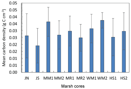
Mean carbon density (blue bars) in grams of carbon per cubic centimeter (g C/cm3) and standard deviations (error bars) for cores collected in five study marshes in Humboldt Bay, California (Curtis and others, 2022). Core abbreviations are provided in figure 12.
Impacts of Marsh Edge Erosion on Blue Carbon Storage
Marsh edge erosion was variable (fig. 15). Edge erosion at Mad River and Manila marshes resulted in the loss of less than 1 percent of the vegetated marsh area. In comparison, edge erosion resulted in the loss of 2.4 and 7.2 percent of the vegetated area at Jacoby and White marshes, respectively (table 11). Jacoby and White marshes are low-elevation marshes with the transition from mudflat to vegetated marsh edge characterized by a gentle gradient (herein referred to as a ramped edge morphology) and more exposure to wind waves, which potentially explains higher edge erosion. A total of 0.44–0.73 hectares (ha) was lost due to edge erosion across all sites between 2010 and 2019. The total mass of soil carbon loss was calculated using the mean carbon density values for each study marsh (fig. 14).
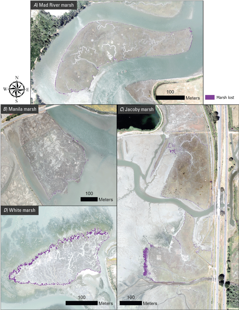
Marsh edge erosion (purple) across A, Mad River; B, Manila; C, Jacoby; and D, White marshes. Background orthoimagery is from 2019 (Office for Coastal Management, 2021c).
Table 11.
Marsh retreat characteristics for each study marsh during water years 2010–19.[The amount of carbon mobilized was estimated by assuming each pixel lost was 0.38 meters (m) deep and contained the average carbon density for the site (Curtis and others, 2022). Abbreviations: ha, hectares; %, percentage; t; metric tons; yr, year; ±, plus or minus]
The depth of eroded soil was difficult to calculate with much accuracy because of the low-point density for the 2010 LiDAR dataset. Low-point density LiDAR is more likely to have returns from the upper part of the vegetation canopy, whereas higher-point density LiDAR may penetrate the canopy more often. Areas experiencing marsh edge erosion at Jacoby marsh had a wide range of elevation differences between the 2010 and 2019 LiDAR datasets. The median difference value was −0.38 m, which was assumed to be the erodible depth across all four marshes. As higher spatial and temporal resolution data become available, this eroded depth value could be improved upon. Repeat monitoring of marsh erosion using imagery, collected with cameras mounted on an uncrewed aerial system (UAS) and structure-from-motion methods (SfM) could be used to create high-resolution topography and vegetation models to detect marsh loss (Stagg and others, 2020).
The impact of edge erosion, the mass of carbon mobilized from the marsh edge, and the impact on carbon storage varied across sites. Carbon mobilization ranged from 0.71 metric tons of carbon per year (t C/yr) at Mad River marsh to 3.46 t C/yr at White marsh (table 11). The largest impact of edge erosion on carbon storage was in the two marshes with the highest fetch and greatest exposure to wind-wave erosion (Jacoby and White marshes). In total, 62.3 t of carbon were estimated to be mobilized (to the atmosphere or other parts of the marsh or mudflat) due to edge erosion during WYs 2010–19. The total mobilization of carbon storage represents only 0.08±0.11percent of the erodible carbon stock across the four sites (assuming a constant 0.38-m erodible depth).
Influence of Sediment Supply and Sea-Level Rise on Marsh Accretion Rates
To offset the combined effects of SLR and tectonic subsidence, salt marshes in Humboldt Bay need a sufficient supply of inorganic sediment to maintain vertical accretion rates. Recent salt marsh studies indicated that sediment transport-based metrics are good indicators of vulnerability and marsh stability (Ganju and others, 2013, 2015).
Marshes located in regions of Humboldt Bay with a higher sediment supply may be more resilient to SLR. Jacoby Creek and Freshwater Creek flow into North Bay and discharge approximately 17 percent of the total annual fine-sediment load delivered to the bay. Elk River flows into Entrance Bay and delivers 35 percent of the annual load. Salmon Creek flows into South Bay and delivers 48 percent of the annual load. On the basis of this relative comparison, it appears that marshes located in South Bay have a higher available sediment supply.
If the mean SSC within the primary tidal channel, which conveys water and sediment to the adjacent marshes where SET-MH sampling occurred, is assumed to be representative of the ambient fine-sediment supply available for marsh accretion, then Hookton Slough is relatively sediment rich. In comparison, lower mean SSC values were computed for Mad River Slough, which appears to be sediment limited with a lower ambient sediment supply available for marsh accretion.
Direct measurements of marsh accretion measured across Humboldt Bay indicated a short-term accretion rate of 1.8±0.6 mm/yr during the monitoring period. This rate is lower than historical accretion rates estimated using marsh cores (3.5–5.7 mm/yr; Thorne and others, 2016). The annual supply of inorganic sediment required to balance the historical accretion rate is 0.010–0.016 t/yr, and this represents 19–30 percent of the annual fine-sediment delivery computed for the local watersheds (0.06±0.02 t/yr; Curtis and others, 2021).
Summary
The data-collection activities summarized in this report were completed by the U.S. Geological Survey in cooperation with the California State Coastal Conservancy, the California Department of Fish and Wildlife, and the U.S. Fish and Wildlife Service—Humboldt Bay National Wildlife Refuge. Results and interpretations presented in this report will support sea-level rise (SLR) adaptation planning and will help resource managers develop and implement sediment-based strategies (salt marsh restoration, regional sediment management, and beneficial reuse of dredged material) to build coastal resiliency to climate change.
Understanding the linkages between water-quality conditions, salt marsh accretion processes, and soil-carbon storage can help inform management actions related to managing blue carbon stocks, and assessing marsh vulnerability to sea-level rise. Water-quality conditions (temperature, salinity, turbidity, and suspended-sediment concentration), and salt marsh processes (duration of flooding of the marsh surface, surface deposition, elevation change, and edge erosion) varied across the study marshes and within different regions of Humboldt Bay. In comparison, the five salt marshes were similar with respect to percent organic carbon content and carbon density.
Suspended-sediment concentration is a limiting factor for marsh accretion. Throughout the monitoring period, higher suspended-sediment concentrations were measured at the South Bay water-quality monitoring station, located in Hookton Slough. In South Bay, a larger fluvial sediment supply and higher ambient SSC conditions appear to provide a larger suspended-sediment supply to support marsh accretion and offset the effects of SLR.
South Bay is a sediment-rich region that receives 48 percent of the fine-sediment delivery from local watersheds that discharge fluvial sediment directly to Humboldt Bay. The mean suspended-sediment concentration computed for the Hookton Slough station (USGS station 404038124131801) was 50.7±22.2 milligrams per liter (mg/L), with uncertainty estimated using the 90-percent confidence interval computed for the surrogate regression model. In comparison, North Bay is a sediment-limited region that receives only 17 percent of the total fine-sediment delivery from local fluvial sources. The mean SSC computed for the Mad River Slough station (USGS station 405219124085601) was 17.8±6.8 mg/L. The differences in SSC between Mad River Slough and Hookton Slough are consistent with differences in surface deposition rates measured in the adjacent study marshes. The average annual surface deposition rates were 1.1±0.4 millimeters per year (mm/yr) for Mad River marsh and 4.2±0.3 mm/yr for Hookton marsh.
Rates of marsh surface deposition and elevation change varied across the study marshes. The mean rate of surface deposition for the North Bay marshes (Mad River, Manila, and Jacoby) was 1.9±0.5 mm/yr, and the mean rate of elevation change was 1.1±0.8 mm/yr. In comparison, the mean rate of surface deposition was 3.5±0.7 mm/yr for the South Bay marshes (White and Hookton), and the mean rate of elevation change was 2.9±0.5 mm/yr. Across Humboldt Bay marshes, surface deposition rates were greater than rates of elevation change, indicating that shallow subsidence related to decomposition or compaction could be a limiting factor that influences vertical accretion and the ability to offset the effects of SLR. During the monitoring period, short-term rates of elevation change across Humboldt Bay were less than the published long-term rates of local sea-level rise (4.9 mm/yr). In general, caution should be used when comparing short-term records of surface deposition and elevation change within the context of long-term trends in SLR. For example, stochastic events (such as atmospheric rivers) can deliver sediment subsidies that offset the impacts of SLR.
Marsh edge erosion and the resulting impacts on soil carbon storage varied across the study marshes. Lower elevation marshes, with the transition from mudflat to marsh edge characterized by a gentle gradient (herein, ramped edge morphology) and larger wind-wave exposure, experienced higher rates of marsh edge erosion and greater soil carbon loss. Losses of soil carbon due to marsh edge erosion ranged from 0.71 metric tons of carbon per year (Mad River marsh) to 3.46 metric tons year of carbon per year (White marsh). In total, marsh edge erosion was responsible for the loss of 62.3 metric tons of the blue carbon stock stored in four study marshes.
This report summarized less than 5 years of water-quality and salt marsh monitoring data. These short-term results represent initial baseline measurements and should be interpreted with caution because long-term monitoring may show different results. Continued monitoring over a decade or longer is typically required to capture wet and dry years and stochastic events and to understand long-term trends.
References Cited
American Society for Testing and Materials, 2002, Standard test methods for determining sediment concentration in water samples: West Conshohocken, Pa., American Society for Testing and Materials International, D3977-97v. 11.02: Water (Basel), (II): p. 395–400, accessed June 1, 2021, at https://www.astm.org/d3977-97r19.html.
Anderson, C.W., 2005, Turbidity: U.S. Geological Survey Techniques of Water-Resources Investigations, book 9, chap. A6.7, accessed June 1, 2021, at https://doi.org/10.3133/twri09A6.7.
Association of Official Analytical Chemists, 1997, Official method 972.43, Microchemical determination of Carbon, Hydrogen, and Nitrogen, automated method—Official Methods of Analysis of AOAC International (16th ed.): Arlington, Va., AOAC International, p. 5–6. [Available at https://www.aoac.org/.]
Barnhart, R.A., Boyd, M.J., and Pequegnat, J.E., 1992, The ecology of Humboldt Bay, California—An estuarine profile: U.S. Fish Wildlife Service, Biological Report, v. 68, no. 1, 121 p., accessed June 1, 2021, at https://doi.org/10.1016/0006-3207(94)90583-5.
Brown, L., 2019, California Salt Marsh accretion, ecosystem services, and disturbance responses in the face of climate change: University of California Los Angeles, Ph.D. dissertation, accessed June 1, 2021, at https://escholarship.org/uc/item/3gq3p803#metrics.
Brown, W.M., III, and Ritter, J.R., 1971, Sediment transport and turbidity in the Eel River Basin, California: U.S. Geological Survey Water Supply Paper 1986. [Available at https://doi.org/10.3133/wsp1986.]
Cahoon, D., 1997, Global warming, sea-level rise, and coastal marsh survival: U.S. Geological Survey Fact Sheet 91–97, 2 p., accessed June 1, 2021, at https://doi.org/10.3133/fs09197.
Cahoon, D.R., Lynch, J.C., Hensel, P., Boumans, R., Perez, B.C., Segura, B., and Day, J.W., 2002, High-precision measurements of wetland sediment elevation—I. Recent improvements to the sedimentation-erosion table: Journal of Sedimentary Research, v. 72, no. 5, p. 730–733. [Available at https://doi.org/10.1306/020702720730.]
Cahoon, D.R., Hensel, P.F., Spencer, T., Reed, D.J., Mckee, K.L., and Saintilan, N., 2006, Coastal wetland vulnerability to relative sea-level rise—Wetland elevation trends and process controls, in Verhoeven, J.T.A., Beltman, B., Bobbink, R., and Whigham, D.F., eds., Wetlands and natural resource management: Ecological Studies, v. 190, p. 271–292, accessed June 1, 2021, at https://doi.org/10.1007/978-3-540-33187-2_12.
Cahoon, D.R., McKee, K.L., and Morris, J.T., 2021, How plants influence resilience of salt marsh and mangrove wetlands to sea-level rise: Estuaries and Coasts, v. 44, no. 4, p. 883–898, accessed June 1, 2021, at https://doi.org/10.1007/s12237-020-00834-w.
Callaway, J.C., Nyman, J.A., and DeLaune, R.D., 1996, Sediment accretion in coastal wetlands—A review and a simulation model of processes: Current Topics in Wetland Biogeochemistry, v. 2, p. 2–23. [Available at https://www.researchgate.net/publication/284056250_Sediment_accretion_in_coastal_wetlands_A_review_and_a_simulation_model_of_processes.]
Clarke, S.H., and Carver, G.A., 1992, Late Holocene tectonics and paleoseismicity, southern Cascadia subduction zone: Science, v. 255, no. 5041, p. 188–192, accessed June 1, 2021, at https://doi.org/10.1126/science.255.5041.188.
Cloern, J.E., and Jassby, A.D., 2012, Drivers of change in estuarine-coastal ecosystems—Discoveries from four decades of study in San Francisco Bay: Reviews of Geophysics, v. 50, no. 4, 33 p. [Available at https://doi.org/10.1029/2012RG000397.]
Curtis, J.A., 2021a, Model archive summary for a suspended-sediment concentration surrogate regression model for station 404038124131801; Hookton Slough near Loleta, CA: U.S. Geological Survey data release, accessed June 1, 2021, at https://doi.org/10.5066/P9RJTAIL.
Curtis, J.A., 2021b, Model archive summary for a suspended-sediment concentration surrogate regression model for station 405219124085601; Mad River Slough near Arcata, CA: U.S. Geological Survey data release, accessed June 1, 2021, at https://doi.org/10.5066/P9TVX0Z8.
Curtis, J.A., Freeman, C., and Thorne, K., 2019, Early results—Salt marsh response to changing fine-sediment supply conditions, Humboldt Bay, CA: Reno, Nev., Federal Interagency Sedimentation and Hydrologic Modeling Conference (SEDHYD 2019), June 24–28, 2019, 15 p., accessed June 1, 2021, at https://digitalcommons.humboldt.edu/cgi/viewcontent.cgi?article=1020&context=hsuslri_state.
Curtis, J.A., Flint, L.E., Stern, M.A., Lewis, J., and Klein, R.D., 2021, Amplified impact of climate change on fine-sediment delivery to a subsiding coast, Humboldt Bay, California: Estuaries and Coasts, v. 44, p. 2173–2193, accessed June 1, 2021, at https://doi.org/10.1007/s12237-021-00938-x.
Curtis, J.A., Thorne, K.M., Freeman, C.M., Buffington, K.J., and Drexler, J.Z., 2022, Salt marsh monitoring during water years 2013 to 2019, Humboldt Bay, CA—Water levels, surface deposition, elevation change, and soil carbon storage: U.S. Geological Survey data release, accessed June 1, 2021, at https://doi.org/10.5066/P9QLAL7B.
Crooks, S., Windham-Myers, L., and Troxler, T.G., 2018, Defining blue carbon—The emergence of a climate context for coastal carbon dynamics, chap. 1 of Windham-Myers, L., Crooks, S., and Troxler, T.G., eds., A blue carbon primer—The state of coastal wetland carbon science, practice, and policy: Boca Raton, Fla., CRC Press, p. 1–8, accessed June 1, 2021, at https://doi.org/10.1201/9780429435362.
D’Alpaos, A., Mudd, S.M., and Carniello, L., 2011, Dynamic response of marshes to perturbations in suspended sediment concentrations and rates of relative sea level rise: Journal of Geophysical Research, v. 116, no. F4, 13 p. [Available at https://doi.org/10.1029/2011JF002093.]
Dettinger, M.D., Ralph, F.M., Das, T., Neiman, P.J., and Cayan, D.R., 2011, Atmospheric rivers, floods and the water resources of California: Water, v. 3, no. 2, p. 445–478, accessed June 1, 2021, at https://doi.org/10.3390/w3020445.
Downing, J., 2006, Twenty-five years with OBS sensors—The good, the bad, and the ugly, in Ogston, A.S., Kineke, G.C., and Sherwood, C.R., eds., Special issue in honor of Richard W. Sternberg’s contributions to marine sedimentology: Continental Shelf Research, v. 26, nos. 17–18, p. 2299–2318, accessed June 1, 2021, at https://doi.org/10.1016/j.csr.2006.07.018.
Drexler, J.Z., de Fontaine, C.S., and Deverel, S.J., 2009, The legacy of wetland drainage on the remaining peat in the Sacramento–San Joaquin Delta, California, USA: Wetlands, v. 29, no. 1, p. 372–386, accessed June 1, 2021, at https://doi.org/10.1672/08-97.1.
Druine, F., Verney, R., Deloffre, J., Lemoine, J.P., Chapalain, M., Landemaine, V., and Lafite, R., 2018, In situ high frequency long term measurements of suspended sediment concentration in turbid estuarine system (Seine Estuary, France)—Optical turbidity sensors response to suspended sediment characteristics: Marine Geology, v. 400, p. 24–37, accessed June 1, 2021, at https://doi.org/10.1016/j.margeo.2018.03.003.
Evans, D., Lautenbacher, C.C., Spinrad, R.W., and Szabados, M., 2003, Computational techniques for tidal datums handbook: NOAA Special Publication NOS CO-OPS 2, accessed June 1, 2021, at https://doi.org/10.25607/OBP-190.
Ganju, N.K., Kirwan, M.L., Dickhudt, P.J., Guntenspergen, G.R., Cahoon, D.R., and Kroeger, K.D., 2015, Sediment transport-based metrics of wetland stability: Geophysical Research Letters, v. 42, no. 19, p. 7992–8000, accessed June 1, 2021, at https://doi.org/10.1002/2015GL065980.
Ganju, N.K., Nidzieko, N.J., and Kirwan, M.L., 2013, Inferring tidal wetland stability from channel sediment fluxes—Observations and a conceptual model: Journal of Geophysical Research. Earth Surface, v. 118, no. 4, p. 2045–2058. [Available at https://doi.org/10.1002/jgrf.20143.]
Geyer, W.R., and MacCready, P., 2014, The estuarine circulation: Annual Review of Fluid Mechanics, v. 46, p. 175–197, accessed June 1, 2021, at https://doi.org/10.1146/annurev-fluid-010313-141302.
Harris, D., Horwáth, W.R., and van Kessel, C., 2001, Acid fumigation of soils to remove carbonates prior to total organic carbon or carbon-13 isotopic analysis: Soil Science Society of America Journal, v. 65, no. 6, p. 1853–1856, accessed June 1, 2021, at https://doi.org/10.2136/sssaj2001.1853.
Helsel, D.R., Hirsch, R.M., Ryberg, K.R., Archfield, S.A., and Gilroy, E.J., 2020, Statistical methods in water resources: U.S. Geological Survey Techniques and Methods, book 4, chap. A3, 458 p., accessed June 1, 2021, at https://doi.org/10.3133/tm4A3.
Holmes, R.R., Terrio, P.J., Harris, M.A., and Mills, P.C., 2001, Introduction to field methods for hydrologic and environmental studies: U.S. Geological Survey Open File Report 2001–50, 241 p., accessed June 1, 2021, at https://doi.org/10.3133/ofr0150.
Holmquist, J.R., Windham-Myers, L., Bliss, N., Crooks, S., Morris, J.T., Megonigal, J.P., Troxler, T., Weller, D., Callaway, J., Drexler, J., Ferner, M.C., Gonneea, M.E., Kroeger, K.D., Schile-Beers, L., Woo, I., Buffington, K., Breithaupt, J., Boyd, B.M., Brown, L.N., Dix, N., Hice, L., Horton, B.P., MacDonald, G.M., Moyer, R.P., Reay, W., Shaw, T., Smith, E., Smoak, J.M., Sommerfield, C., Thorne, K., Velinsky, D., Watson, E., Grimes, K.W., and Woodrey, M., 2018, Accuracy and precision of tidal wetland soil carbon mapping in the conterminous United States: Scientific Reports, v. 8, no. 9478, 16 p. [Available at https://doi.org/10.1038/s41598-018-26948-7.]
Janousek, C.N., Dugger, B.D., Drucker, B.M., and Thorne, K.M., 2020, Salinity and inundation effects on productivity of brackish tidal marsh plants in the San Francisco Bay-Delta Estuary: Hydrobiologia, v. 847, p. 4311–4323, accessed June 1, 2021, at https://doi.org/10.1007/s10750-020-04419-3.
Kelsey, H.M., 1980, A sediment budget and an analysis of geomorphic process in the Van Duzen River basin, north coastal California, 1941–1975—Summary: Geological Society of America Bulletin, Part I, v. 91, no. 4, p. 190–195, accessed June 1, 2021, at https://doi.org/10.1130/0016-7606(1980)91<190:ASBAAA>2.0.CO;2.
Kirwan, M.L., Guntenspergen, G.R., D’Alpaos, A., Morris, J.T., Mudd, S.M., and Temmerman, S., 2010, Limits on the adaptability of coastal marshes to rising sea level: Geophysical Research Letters, v. 37, no. 23, 5 p. [Available at https://doi.org/10.1029/2010GL045489.]
Klein, R.D., Lewis, J., and Buffleben, M.S., 2012, Logging and turbidity in the coastal watersheds of northern California: Geomorphology, v. 139–140, p. 136–144, accessed June 1, 2021, at https://doi.org/10.1016/j.geomorph.2011.10.011.
Leithold, E.L., Perkey, D.W., Blair, N.E., and Creamer, T.N., 2005, Sedimentation and carbon burial on the northern California continental shelf—The signatures of land-use change: Continental Shelf Research, v. 25, no. 3, p. 349–371, accessed June 1, 2021, at https://doi.org/10.1016/j.csr.2004.09.015.
Leonardi, N., Ganju, N.K., and Fagherazzi, S., 2016, A linear relationship between wave power and erosion determines salt-marsh resilience to violent storms and hurricanes: Proceedings of the National Academy of Sciences, v. 113, no. 1, p. 64–68, accessed June 1, 2021, at https://doi.org/10.1073/pnas.1510095112.
Lynch, J.C., Hensel, P., and Cahoon, D.R., 2015, The surface elevation table and marker horizon technique—A protocol for monitoring wetland elevation dynamics: Fort Collins, Colo., Natural Resource Report NPS/NCBN/NRR-2015/1078, National Park Service, accessed June 1, 2021, at https://pubs.er.usgs.gov/publication/70160049.
Mcleod, E., Chmura, G.L., Bouillon, S., Salm, R., Björk, M., Duarte, C.M., Lovelock, C.E., Schlesinger, W.H., and Silliman, B.R., 2011, A blueprint for blue carbon—Toward an improved understanding of the role of vegetated coastal habitats in sequestering CO2: Frontiers in Ecology and the Environment, v. 9, no. 10, p. 552–560, accessed June 1, 2021, at https://doi.org/10.1890/110004.
Milliman, J.D., and Farnsworth, K.L., 2011, River discharge to the coastal ocean—A global synthesis: Cambridge, UK, Cambridge University Press, 384 p., accessed June 1, 2021, at https://doi.org/10.1017/CBO9780511781247.
Montillet, J.P., Melbourne, T.I., and Szeliga, W.M., 2018, GPS vertical land motion corrections to sea-level rise estimates in the Pacific Northwest: Journal of Geophysical Research. Oceans, v. 123, no. 2, p. 1196–1212. [Available at https://doi.org/10.1002/2017JC013257.]
Morris, J.T., Sundareshwar, P.V., Nietch, C.T., Kjerfve, B., and Cahoon, D.R., 2002, Responses of coastal wetlands to rising sea level: Ecology, v. 83, no. 10, p. 2869–2877, accessed June 1, 2021, at https://doi.org/10.1890/0012-9658(2002)083[2869:ROCWTR]2.0.CO;2.
National Centers for Environmental Information, 2022, Rainfall for Eureka, California, GHCND: USW00024213: National Centers for Environmental Information webpage, accessed March 18, 2022, at https://www.ncei.noaa.gov/.
National Oceanic and Atmospheric Administration, 2022a, Relative sea level trend for 9418767, North Spit, California: NOAA Tides and Currents webpage, accessed March 18, 2022, at https://tidesandcurrents.noaa.gov/sltrends/sltrends_station.shtml?id=9418767.
National Oceanic and Atmospheric Administration, 2022b, Datums for 9418767, North Spit, California: NOAA Tides and Currents webpage, accessed March 18, 2022, at https://tidesandcurrents.noaa.gov/datums.html?id=9418767.
Nellemann, C., Corcoran, E., Duarte, C.M., Valdés, L., De Young, C., Fonseca, L., and Grimsditch, G., 2009, Blue carbon—The role of healthy oceans in binding carbon: Rapid Response Assessment UN Environment, GRID-Arendal, accessed June 1, 2021, at https://www.grida.no/publications/145.
Nicholls, R.J., 2018, Adapting to sea-level rise, chap. 2 of Zommers, Z., and Alverson, K., eds., Resilience—The science of adaptation to climate change: Elsevier, p. 13–29, accessed June 1, 2021, at https://doi.org/10.1016/B978-0-12-811891-7.00002-5.
Northern Hydrology & Engineering, 2015, Humboldt Bay—Sea level rise, hydrodynamic modeling, and inundation vulnerability mapping: Final Report prepared for State Coastal Conservancy and Coastal Ecosystems Institute of Northern California, 106 p., accessed June 1, 2021, at https://digitalcommons.humboldt.edu/cgi/viewcontent.cgi?article=1004&context=hsuslri_local.
OCM Partners, 2021, 2019 lidar—City of Eureka, CA: NOAA Fisheries webpage, accessed June 1, 2021, at https://www.fisheries.noaa.gov/inport/item/59069.
Office for Coastal Management, 2021a, 2009–2011 CA Coastal conservancy coastal lidar project: NOAA Fisheries webpage, accessed June 1, 2021, at https://www.fisheries.noaa.gov/inport/item/48166.
Office for Coastal Management, 2021b, Coastal California digital imagery: NOAA Fisheries webpage, accessed June 1, 2021, at https://www.fisheries.noaa.gov/inport/item/48416.
Office for Coastal Management, 2021c, 2019 Eureka, CA UltraCam 4-Band 8 Bit Imagery: NOAA Fisheries webpage, accessed June 1, 2021, at https://www.fisheries.noaa.gov/inport/item/58883.
Patrick, W.H., Jr, and DeLaune, R., 1990, Subsidence, accretion, and sea level rise in South San Francisco Bay marshes: Limnology and Oceanography, v. 35, no. 6, p. 1389–1395, accessed June 1, 2021, at https://doi.org/10.4319/lo.1990.35.6.1389.
R Core Team, 2019, R—A language and environment for statistical computing: Vienna, Austria, R Foundation for Statistical Computing, accessed June 1, 2021, at https://www.R-project.org/.
Rasmussen, P.P., Gray, J.R., Glysson, G.D., and Ziegler, A.C., 2009, Guidelines and procedures for computing time-series suspended-sediment concentrations and loads from in-stream turbidity-sensor and streamflow data: U.S. Geological Survey Techniques and Methods, book 3, chap. C4, 52 p., accessed June 1, 2021, at https://pubs.er.usgs.gov/publication/tm3C4.
Roussel, J., and Auty, D., 2020, lidR—Airborne LiDAR data manipulation and visualization for forestry applications: R package, version 2.2.4, accessed June 1, 2021, at https://cran.r-project.org/web/packages/lidR/index.html.
Rovere, A., Stocchi, P., and Vacchi, M., 2016, Eustatic and relative sea level changes, in Horton, B.P., ed., Topical collection on sea level projections: Current Climate Change Reports, v. 2, no. 4, p. 221–231, accessed June 1, 2021, at https://doi.org/10.1007/s40641-016-0045-7.
Russell, N., and Griggs, G., 2012, Adapting to sea level rise—A guide for California’s coastal communities: Prepared for the California Energy Commission Public Interest Environmental Research Program, University of California Santa Cruz, 50 p., accessed June 1, 2021, at http://climate.calcommons.org/bib/adapting-sea-level-rise-guide-california%E2%80%99s-coastal-communities.
Schlosser, S., and Eicher, A., 2012, The Humboldt Bay and Eel River Estuary benthic habitat project: California Sea Grant Publication T-075, 246 p., accessed June 1, 2021, at https://digitalcommons.humboldt.edu/hsuslri_local/24/.
Shepard, C.C., Crain, C.M., and Beck, M.W., 2011, The protective role of coastal marshes—A systematic review and meta-analysis: PLoS One, v. 6, no. 11, 11 p. [Available at https://doi.org/10.1371/journal.pone.0027374.]
Stagg, C.L., Osland, M.J., Moon, J.A., Hall, C.T., Feher, L.C., Jones, W.R., Couvillion, B.R., Hartley, S.B., and Vervaeke, W.C., 2020, Quantifying hydrologic controls on local-and landscape-scale indicators of coastal wetland loss: Annals of Botany, v. 125, no. 2, p. 365–376, accessed June 1, 2021, at https://doi.org/10.1093/aob/mcz144.
Stralberg, D., Brennan, M., Callaway, J.C., Wood, J., Schile, L., Jongsomjit, D., Kelly, M., Parker, V.T., and Crooks, S., 2011, Evaluating tidal marsh sustainability in the face of sea-level rise—A Hybrid modeling approach applied to San Francisco Bay: PLoS One, v. 6, no. 11, 18 p. [Available at https://doi.org/10.1371/journal.pone.0027388.]
Takekawa, J.Y., Thorne, K.M., Buffington, K.J., Freeman, C.M., Powelson, K.W., and Block, G., 2013, Assessing marsh response from sea-level rise applying local site conditions—Humboldt Bay National Wildlife Refuge: Vallejo, Calif., Unpublished Data Summary Report, U.S. Geological Survey Western Ecological Research Center, 44 p. + appendices, accessed June 1, 2021, at https://digitalcommons.humboldt.edu/cgi/viewcontent.cgi?article=1016&context=hsuslri_state.
Thom, R.M., 1992, Accretion rates of low intertidal salt marshes in the Pacific Northwest: Wetlands, v. 12, no. 3, p. 147–156, accessed June 1, 2021, at https://doi.org/10.1007/BF03160603.
Thorne, K.M., MacDonald, G.M., Ambrose, R.F., Buffington, K.J., Freeman, C.M., Janousek, C.N., Brown, L.N., Holmquist, J.R., Guntenspergen, G.R., Powelson, K.W., Barnard, P.L., and Takekawa, J.Y., 2016, Effects of climate change on tidal marshes along a latitudinal gradient in California: U.S. Geological Survey Open-File Report 2016–1125, 75 p., accessed June 1, 2021, at https://doi.org/10.3133/ofr20161125.
Thorne, K.M., MacDonald, G., Guntenspergen, G., Ambrose, R., Buffington, K., Dugger, B., Freeman, C., Janousek, C., Brown, L., Rosencranz, J., Holmquist, J., Smol, J., Hargan, K., and Takekawa, J., 2018, U.S. Pacific coastal wetland resilience and vulnerability to sea-level rise: Science Advances, v. 4, no. 2, 10 p. [Available at https://doi.org/10.1126/sciadv.aao3270.]
U.S. Geological Survey, 2021, USGS water data for the Nation: U.S. Geological Survey National Water Information System database, accessed June 1, 2021, at https://doi.org/10.5066/F7P55KJN.
Valentine, D.W., Keller, E.A., Carver, G., Li, W.H., Manhart, C., and Simms, A.R., 2012, Paleoseismicity of the southern end of the Cascadia subduction zone, northwestern California: Bulletin of the Seismological Society of America, v. 102, no. 3, p. 1059–1078, accessed June 1, 2021, at https://doi.org/10.1785/0120110103.
Wagner, R.J., Boulger, R.W., Jr., Oblinger, C.J., and Smith, B.A., 2006, Guidelines and standard procedures for continuous water-quality monitors—Station operation, record computation, and data reporting: U.S. Geological Survey Techniques and Methods, book 1, chap. D3, 51 p., accessed June 1, 2021, at https://doi.org/10.3133/tm1D3.
Warrick, J.A., Madej, M.A., Goñi, M.A., and Wheatcroft, R.A., 2013, Trends in the suspended-sediment yields of coastal rivers of northern California, 1955–2010: Journal of Hydrology, v. 489, p. 108–123. [Available at https://doi.org/10.1016/j.jhydrol.2013.02.041.]
Webb, E.L., Friess, D.A., Krauss, K.W., Cahoon, D.R., Guntenspergen, G.R., and Phelps, J., 2013, A global standard for monitoring coastal wetland vulnerability to accelerated sea-level rise: Nature Climate Change, v. 3, p. 458–465, accessed June 1, 2021, at https://doi.org/10.1038/nclimate1756.
Weston, N.B., 2014, Declining sediments and rising seas—An unfortunate convergence for tidal wetlands: Estuaries and Coasts, v. 37, no. 1, p. 1–23, accessed June 1, 2021, at https://doi.org/10.1007/s12237-013-9654-8.
Xu, J., Myers, E., and White, S., 2010, VDatum for the coastal waters of north/central California, Oregon and western Washington—Tidal datums and sea surface topography: NOAA Technical Memorandum NOS CS 22, accessed June 1, 2021, at http://vdatum.noaa.gov/.
Conversion Factors
International System of Units to U.S. customary units
Temperature in degrees Celsius (°C) may be converted to degrees Fahrenheit (°F) as follows:
°F = (1.8 × °C) + 32.
Datums
Vertical coordinate information is referenced to the North American Vertical Datum of 1988 (NAVD 88).
Horizontal coordinate information is referenced to the North American Datum of 1983 (NAD 83).
Tidal datums at station 9418767 (https://tidesandcurrents.noaa.gov/datums.html?id=9418767) are typically referenced to Mean Lower Low Water (MLLW; computed for epoch 1983–2001), where MLLW is at 0 meters (m). In this report, tidal datums are referenced to meters above NAVD 88. At station 9418767, MLLW is at 0.10 meters above NAVD 88, and Mean Higher High Water is at 2.19 meters above NAVD 88.
Supplemental Information
Specific conductance is reported in microsiemens per centimeter at 25 degrees Celsius (µS/cm at 25 °C). Salinity is reported in practical salinity units (PSU). Turbidity is reported in formazin nephelometric units (FNU). Concentrations of chemical constituents in water are reported in either milligrams per liter (mg/L) or parts per million (ppm). Annual supply of fine-grained (less than 63 µm) inorganic sediment is reported in metric tons per year (t/yr). Light Detection and Ranging (LiDAR) point densities are reported in points per square meter (pt/m2). Mean carbon density is reported in grams of carbon per cubic centimeter (g C/cm3). Mobilization of carbon by marsh edge erosion is reported in metric tons of carbon per year (t C/yr).
Abbreviations
ANOVA
analysis of variance
BCF
bias correction factor
LiDAR
light detection and ranging
MH
marker horizon
MHHW
mean higher-high water
MHW
mean high water
MLLW
mean lower-low water
MLW
mean low water
MSPE
mean standard percent error
MTL
mean tide level
NDVI
normalized difference vegetation index
NWIS
National Water Information System
R2
coefficient of determination
RTK-GNSS
real-time kinematic global navigation satellite systems
SET
surface elevation table
SLR
sea-level rise
SSC
suspended-sediment concentration
USGS
U.S. Geological Survey
WY
water year (October 1 to September 30, defined by year in which it ends)
For more information concerning the research in this report, contact the
Director, California Water Science Center
U.S. Geological Survey
6000 J Street, Placer Hall
Sacramento, California 95819
https://www.usgs.gov/centers/ca-water/
Publishing support provided by the U.S. Geological Survey
Science Publishing Network, Sacramento Publishing Service Center
Suggested Citation
Curtis, J.A., Thorne, K.M., Freeman, C.M., Buffington, K.J., and Drexler, J.Z., 2022, A summary of water-quality and salt marsh monitoring, Humboldt Bay, California: U.S. Geological Survey Open-File Report 2022–1076, 30 p., https://doi.org/10.3133/ofr20221076.
ISSN: 2331-1258 (online)
Study Area
| Publication type | Report |
|---|---|
| Publication Subtype | USGS Numbered Series |
| Title | A summary of water-quality and salt marsh monitoring, Humboldt Bay, California |
| Series title | Open-File Report |
| Series number | 2022-1076 |
| DOI | 10.3133/ofr20221076 |
| Year Published | 2022 |
| Language | English |
| Publisher | U.S. Geological Survey |
| Publisher location | Reston, VA |
| Contributing office(s) | California Water Science Center, Western Ecological Research Center |
| Description | Report: viii, 30 p.; 3 Data Releases |
| Country | United States |
| State | California |
| Other Geospatial | Humboldt Bay |
| Online Only (Y/N) | Y |
| Additional Online Files (Y/N) | Y |
| Google Analytic Metrics | Metrics page |