

Evaluation of the Bushy Park Reservoir Three-Dimensional Hydrodynamic and Water-Quality Model, South Carolina, 2012–15
Links
- Document: Report (5.22 MB pdf) , HTML , XML
- Data Release: USGS data release - Water quality data for Bushy Park Reservoir, South Carolina 2013–2015
- Download citation as: RIS | Dublin Core
Acknowledgments
The authors thank the staff of Charleston Water System (CWS) and, in particular, Kin Hill, Chief Executive Officer, Andy Fairey, Chief Operating Officer, and Jane Bryne, Director of Water Treatment, for their technical assistance and coordination during this study. The authors also thank Mark Valerio of South Carolina Electric and Gas for the daily Williams Station plant operating data and Rebecca Thames of CWS for providing laboratory data. The authors also thank the CWS and U.S. Geological Survey reviewers for their thoughtful reviews and constructive comments of this report. At the time of publication, Tetra Tech data from the Bushy Park model were unavailable; for more information on the model, contact Charleston Water System.
Abstract
The Bushy Park Reservoir is a relatively shallow impoundment in southeastern South Carolina. The reservoir, located under a semi-tropical climate, is the principal water supply for the city of Charleston, South Carolina, and the surrounding areas including the Bushy Park Industrial Complex. Although there was an adequate supply of freshwater in the reservoir in 2022, water-quality concerns are present over taste-and-odor and saltwater-intrusion issues. From 2013 to 2015, the U.S. Geological Survey (USGS), in cooperation with the Charleston Water System, engaged in a multi-year study of the hydrology and hydrodynamics of Bushy Park Reservoir to better understand factors affecting water-quality conditions in the reservoir. As part of this study, Charleston Water System worked with Tetra Tech, Inc., a consulting and engineering firm, to develop a Bushy Park Reservoir hydrodynamic and water-quality modeling framework, built upon earlier efforts by both Tetra Tech and the U.S. Army Corps of Engineers. At the completion of the new modeling framework, the USGS was requested to evaluate the calibrated hydrodynamic and water-quality model.
The Bushy Park Reservoir Environmental Fluid Dynamics Code (EFDC) model was calibrated for the time period from January 1, 2012, to December 31, 2015. The general modeling approach for the newly revised modeling framework, as briefly detailed in this report, was developed with EFDC. The EFDC is a grid-based modeling package that can simulate three-dimensional flow, transport, and water quality in surface-water systems. This report evaluated the capacity of Tetra Tech’s Bushy Park EFDC model to simulate water discharge, water circulation, surface elevations, temperature, salinity, and other water-quality parameters.
The USGS model review focused specifically on the following criteria: (1) determine if the model, with additional effort, could be developed into an adequate planning tool for Bushy Park Reservoir; (2) assess the capacity of the model to specifically address water-quality issues in the reservoir related to taste-and-odor and saltwater intrusions; and, (3) evaluate three preliminary water-management scenarios related to reduced water withdrawals in the reservoir and the effect on saltwater intrusion.
Overall, the model was able to simulate discharge, flow velocity, and water-surface elevations with generally good agreement between the simulated and measured values. Specifically, the model was able to demonstrate good agreement for discharge at two USGS continuous discharge locations (USGS station 02172002; USGS station 02172040), with Wilmott index of agreements of 0.86 and 0.75, respectively. A total of seven USGS streamgages, located on the West Branch of the Cooper River, Durham Canal, and the Cooper River, were available for water-surface elevations, with index of agreements ranging from 0.74 to 0.99. However, model-simulated water-surface elevation ranges were appreciably high (compared to measured ranges) for two locations near Pinopolis Dam, farthest upstream on the West Branch of the Cooper River. This result may indicate that too much simulated tidal energy propagated through the model domain.
For water temperature, 16 calibration stations were available for at least part of the 4-year simulation. The index of agreement range for temperature comparisons was from 0.95 to 1.00, indicating excellent agreement between the measured and simulated results. One of the primary future applications for the Bushy Park Reservoir EFDC model is to determine the extent of saltwater intrusions. A wide range in the salinity prediction quality was simulated with the model. The prediction quality ranged from an index of agreement of 0.15 at Cooper River approximately 2.75 miles southeast of the Tee, South Carolina, to 0.92 at West Branch Cooper River near Moncks Corner, South Carolina. Although the model did not accurately simulate some of the larger salinity deviations resulting during individual hydrologic events, the seasonal salinity trends were adequately simulated with the model during the study period (2012–15). Therefore, it may be difficult to simulate extreme hydrologic events, such as during large storms, where high salinity water is exchanged with Bushy Park Reservoir. There was agreement in model simulation with the measured data either on the quantitative index of agreement values or qualitative agreement in the seasonal salinity data trends.
For water quality, the index of agreement values were generally low for total nitrogen, ammonia, nitrate, total Kjeldahl nitrogen, total phosphorus, and orthophosphate. Although general trends were adequately simulated at specific stations, particularly for Bushy Park Reservoir, the model-simulated fit was low across all the constituents described above with index of agreements usually below 0.50. A limitation for simulating nutrient concentrations across the model domain was the lack of characterization for the constituents directly entering Bushy Park Reservoir, or the lack of data directly attributed to the boundary condition (for example, the Cooper River). The other two calibrated water-quality constituents (besides the nutrients mentioned above) were dissolved oxygen and chlorophyll a. Dissolved oxygen varied from index of agreement values from 0.58 to 0.94 for 11 stations, generally indicating agreement with the available measured data. Chlorophyll a, calibrated for seven stations, had a wider range from 0.11 to 0.74 for the index of agreement.
With the current modeling framework, taste-and-odor events, related to cyanobacterial blooms, cannot be directly simulated. However, indirect estimates of cyanobacteria concentrations may be obtained by using the chlorophyll a model outputs, which represent total phytoplankton biomass, and the phytoplankton biovolume data by group (diatoms, green algae, cyanobacteria and others) collected from 2012 to 2015. For the Bushy Park Reservoir modeling framework to be used directly for taste-and-odor issues, cyanobacteria must be simulated and calibrated based on observations of cyanobacteria biomass concentrations. In addition to the cyanobacteria sampling conducted within the reservoir between 2012 and 2015, the new model calibration would also require new algae biomass data-collection efforts to characterize the external sources of cyanobacteria entering the Bushy Park Reservoir from tributaries, as well as the internal cycling, production, and decay of cyanobacteria in the hydrologic system.
Further improvements to the EFDC model would include expanding the collection of boundary condition datasets, such as water-quality monitoring to determine improved nutrient loads into the model domain. Along with improved water-quality monitoring for the major boundary conditions, continuous discharge, for both Foster Creek and the Back River, would further constrain the flow balance and the loads into Bushy Park Reservoir. In addition to better boundary-condition characterization, it is important to better characterize possible shortcomings specifically to the model domain, such as the grid resolution, bathymetry, and numerical hydrodynamic errors. Further consideration of the model may involve a sensitivity analysis to determine if errors in the simulation outputs, such as discharge, water-surface elevations, and salinity, were more likely caused by poor boundary condition characterization or, specifically, the model setup.
Three model scenarios were run with the revised Bushy Park Reservoir model: (1) reduced withdrawals from one of the large intake-discharge locations for Bushy Park Reservoir, the Williams Station; (2) elevated (above background levels) ocean water level causing saltwater intrusion from the ocean through Durham Canal into Bushy Park Reservoir; and (3) overtopping of the Back River Dam at the southernmost end of Bushy Park Reservoir. For the reduced withdrawals scenarios, the largest shift in flow resulted near the Williams Station intake, with the next largest flow change at the southern end of Bushy Park Reservoir, and a net increase in flow out of the Bushy Park Reservoir to the Cooper River by way of the Durham Canal. The effect resulting from scenario 3 on water quality and salinity was small, with larger increases for dissolved oxygen than other constituents at several monitoring stations. For the two scenarios related to saltwater intrusion (including dam overtopping), the changes in salinity generally were found to dissipate in the following 2 weeks and generally back to baseline salinity conditions within 3 months. This result did vary depending on the severity of the storm or length of the dam overtopping event.
Introduction
The Charleston Water System (CWS) (formerly the Commissioners of Public Works of the City of Charleston, South Carolina) has been a leader in water-resource planning for the low country of South Carolina since its inception as Charleston Light and Water Company in 1902. In anticipation of the expansion of industrial areas and future water demands, CWS contributed to the construction of the Bushy Park Reservoir and Industrial Complex in the 1950s (Williams, 2010). In 1954, the Bushy Park Industrial Complex was established between the east bank of the Back River and the west bank of the Cooper River and part of the Santee-Cooper River Basin. To provide water to the industrial users, a freshwater reservoir was constructed by damming the Back River at the lower end near the confluence with the Cooper River (fig. 1).
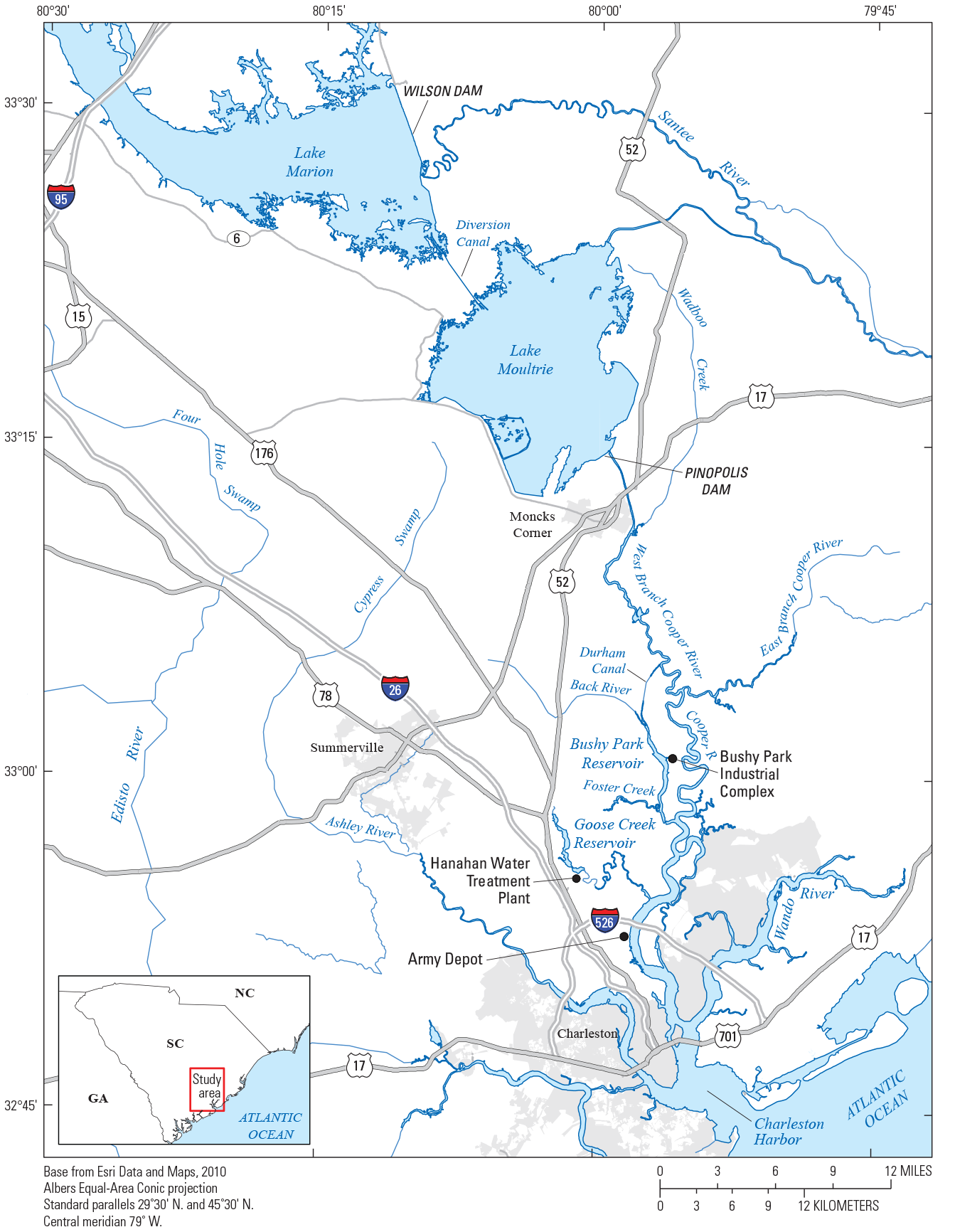
Study area of the Santee-Cooper River Basin, South Carolina.
Bushy Park Reservoir is a relatively shallow impoundment under a semi-tropical climate. Although there is an adequate supply of freshwater present (2022), there are water-quality concerns of taste-and-odor and salinity-intrusion issues. In general, taste-and-odor issues are common in reservoirs used for drinking water throughout the United States (Paerl and others, 2001; Taylor and others, 2006; Jüttner and Watson, 2007), and can often be correlated with the presence of trans-1, 10-dimethyl-trans-decalol (geosmin) and 2-methylisoborneol (MIB). It has been shown that there is a constant production of geosmin and MIB in portions of Bushy Park Reservoir, based on previous sampling by the U.S. Geological Survey (USGS; Conrads and others, 2018). In water bodies, such as Bushy Park Reservoir (fig. 1), the production and release of geosmin and MIB have been related to soil bacteria (actinomycetes) (Jüttner and Watson, 2007) and certain species of cyanobacteria (also known as blue-green algae). Geosmin- and MIB-producing cyanobacteria blooms are attributed to a range of environmental factors, including elevated (above background levels) nutrient concentrations and ratios, light availability, water temperatures, water-column stability, and flushing rates (Downing and others, 2001; Paerl and others, 2001; Mau and others, 2004; Dzialowski and others, 2009). However, the complex interaction among the physical, chemical, and biological processes within lakes and reservoirs often makes it difficult to identify primary environmental factors that cause the production and release of these cyanobacterial by-products. Understanding of the environmental factors that affect cyanobacteria dominance in reservoirs has allowed water-resource and watershed managers to apply management strategies to prevent conditions where cyanobacteria dominate (Downing and others, 2001; Taylor and others, 2006). Remediation efforts to prevent reservoir conditions that cause cyanobacteria dominance depend on a strong scientific understanding of the mechanisms affecting the algal community (Downing and others, 2001; Taylor and others, 2006).
In addition to taste-and-odor issues, saltwater intrusion is also a water-quality concern for Bushy Park Reservoir. Durham Canal connects the Bushy Park Reservoir to the West Brach of the Cooper River (fig. 1). Because the West Branch of the Cooper River is a tidal river, saline water can move into Bushy Park Reservoir by way of exchange with the canal. Additionally, during extreme storm surges, high salinity water could theoretically overtop the Back River Dam at the southern end of Bushy Park Reservoir. In order to alert water operators in the region to appreciable saltwater-intrusion events, the USGS established a real-time salinity alert network in the 1980s along the Cooper River, the West Branch of the Cooper River, and Durham Canal to continuously monitor the location of the freshwater-saltwater interface (Conrads and others, 2017a).
For both taste-and-odor and saltwater-intrusion issues, the complexity of flow and circulation dynamics for the Bushy Park Reservoir can make it difficult to fully understand how to address these issues. As with many estuarine systems, there can be large changes in flows and water levels on the tidal time scale (less than 13 hours), but on longer time scales (day to weeks), there may be only small changes in net (tidally averaged) flows and water levels. The largest freshwater exchange to Bushy Park Reservoir is through Durham Canal (fig. 1). Although the tidal flows in Durham Canal are approximately plus or minus 4,000 cubic feet per second (ft3/s; Bower and others, 1993), the net daily flow is typically about 1,000 ft3/s. Foster Creek and Back River (fig. 1) are tidal sloughs with negligible daily mean streamflows and only contribute substantial freshwater flows during rain events. Foster Creek can increase from average flows of less than 20 ft3/s to over 400 ft3/s during a rain event (Campbell and Bower, 1996). Further complicating flow patterns, much of the circulation within the reservoir results because of water withdrawals by industrial users. For example, the major withdrawal in the area is by the Williams Station that averages approximately 650 ft3/s for cooling water that discharges to the Cooper River (fig. 2).
One way to better understand the complexity of flow in the Bushy Park Reservoir is through the usage of hydrodynamic and water-quality models. These types of models are commonly used for simulation of water-resource scenarios to evaluate potential changes in hydrology, water-plant operations, and industrial water use. Since the 1990s, various models have been applied to the Cooper River and Charleston Harbor (fig. 1) that include Bushy Park Reservoir (Bower and others, 1993; Conrads and Smith, 1997; Cantrell, 20135). Because model selection, model application, model calibration, model review, and regulatory acceptance can be a resource-intensive effort, it is considered advantageous to adopt available modeling approaches rather than start with a new modeling framework, when possible.
One of the most recent modeling efforts that included Bushy Park Reservoir was developed using the three-dimensional modeling framework Environmental Fluid Dynamics Code (EFDC; Hamrick, 1992). The EFDC model was developed in support of the dissolved oxygen (DO) total maximum daily load (TMDL) for the Ashley, Cooper, and Wando Rivers (fig. 2) (Cantrell, 2013). The model was technically reviewed by the U.S. Environmental Protection Agency (EPA) and the South Carolina Department of Health and Environmental Control (SCDHEC). Furthermore, the U.S. Army Corps of Engineers (USACE) has used the model to evaluate the potential effects of the proposed deepening of Charleston Harbor from 45 to 50 ft on hydrodynamics and water quality (U.S. Army Corps of Engineers, 2015). However, even though the Bushy Park Reservoir was included in the model, modeling emphasis was to simulate DO in areas of concern closer to Charleston Harbor. Additionally, the Bushy Park Reservoir was conceptualized as only two-dimensional in the EFDC model, with a limited number of grid cells to define the entire reservoir extent.
A first step in designing a new evaluation (modeling) tool and modeling framework for the Bushy Park Reservoir would be to incorporate all the reservoir hydrodynamics, including continuous discharge from all sources into the reservoir. Additionally, the modeling tool should include flow dynamics in and out of the West Branch of the Cooper River through Durham Canal, as saltwater frequently moves up the river during storm surges and during the regular tidal cycle. As part of the planning process, CWS approached the USGS-South Atlantic Water Science Center for assistance in evaluating the surface-water circulation of Bushy Park Reservoir and the effect of circulation on water quality. To develop this revised modeling framework, the USGS and Tetra Tech reached agreements with CWS to develop the refined Bushy Park Reservoir hydrodynamic and water-quality modeling framework. Tetra Tech provided technical assistance to CWS for developing the modeling framework, whereas the USGS coordinated data collection and evaluation as part of two separate USGS Scientific Investigations Reports (Conrads and others, 2017a; 2018). Additionally, the USGS was requested to evaluate the calibrated model for the appropriate model application as a planning tool for Bushy Park Reservoir.
Purpose and Scope
The purpose of this report is to describe the evaluation of the appropriateness of the revised three-dimensional hydrodynamic model to simulate discharge, flow velocity, water-surface elevations, water temperature, salinity, and water quality for the Bushy Park Reservoir in southeastern South Carolina. Tetra Tech developed the hydrodynamic model, based on an agreement with CWS, in conjunction with sampling efforts coordinated by the USGS. This Bushy Park Reservoir model, based on the EFDC (Hamrick, 1992) framework, was calibrated using data collected from January 2012 through December 2015. CWS can be contacted for more information on acquiring the model.
Model-run comparisons described here were limited to performing model simulations to determine the general model stability and runtime. Only a limited review of model output compared to results, including comparisons of discharge, flow velocity, water-surface elevations, water temperature, salinity, and water quality, is provided in this report. For the main points described in this report, the model review was focused on the following criteria: (1) determine if the model, with additional effort, could be developed into an adequate planning tool; (2) assess the capacity of the model to specifically address reservoir water quality in relation to taste-and-odor and saltwater intrusion issues; and, (3) evaluate three preliminary water-management scenarios.
Description of the Study Area
The Bushy Park Reservoir is located in the lower part of the Santee-Cooper River Basin. This basin covers approximately 24,000 square miles (mi2) and is the second largest drainage basin on the East Coast (Hughes and others, 2000). Bushy Park Reservoir is eutrophic (excessive nutrient amounts) and is heavily vegetated with aquatic plants that thrive only in freshwater, such as water hyacinth (Eichhornia crassipes), water primrose (Ludwigia hexapetala), and hydrilla (Hydrilla verticillata). The South Carolina Department of Natural Resources routinely applies herbicides to mitigate the aquatic growth. Further details of the climate and watershed characteristics are fully described by Conrads and others (2017a, 2018).10
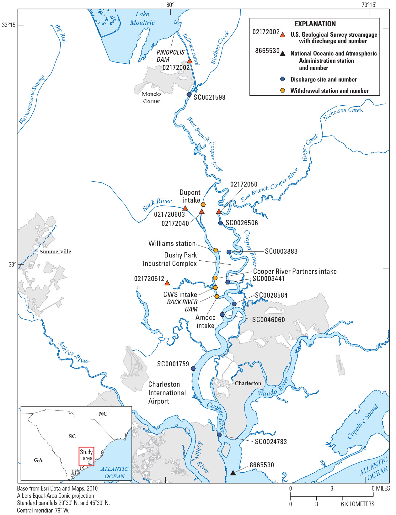
U.S. Geological Survey real-time streamgaging network with discharge (plus one National Oceanic and Atmospheric Administration station) near the Bushy Park Reservoir and the Charleston Water System (CWS), South Carolina, including the eight National Pollution Discharge Elimination System (NPDES) and five withdrawal intakes included in the Bushy Park Reservoir model.
The construction of the Bushy Park Reservoir and Durham Canal is part of the long history of anthropogenic changes to the Santee and Cooper Rivers (fig. 1) (Kjerfve, 1976), going back to the 18th century and early 19th century. The Bushy Park Reservoir was completed to provide a convenient freshwater reservoir for industrial and municipal water use for the newly created Bushy Park Industrial Complex in 1954. As part of the project, the Back River Dam and Durham Canal (fig.1) were built in 1955 and 1956, respectively, by the Bushy Park Authority to form Bushy Park Reservoir. The Back River was dammed at the lower end near the confluence with the Cooper River to create the Bushy Park Reservoir, and Durham Canal was constructed as a conduit between the upper end of the reservoir and the freshwater part of the West Branch of the Cooper River (fig. 1). Charleston County Public Works purchased the assets of the Bushy Park Authority in 1964 and controls use of the waters from the reservoir. Presently (2022), five facilities have water-withdrawal intakes (fig. 2) located on Bushy Park Reservoir including the Dominion Energy Williams Station, CWS, DAK Americas, BP/Amoco (currently Ineos) and Cooper River Partners.
The flow and circulation dynamics of the Bushy Park Reservoir are complex. The major natural tributaries to the Bushy Park Reservoir are the Back River (upstream from the confluence with Durham Canal) and Foster Creek, which contain approximately 12,900 acres (20.2 mi2) of swampy areas (Conrads and others, 2017a). Most of the flow into the Bushy Park Reservoir, however, comes from Durham Canal. The reservoir is tidally affected with resulting semi-diurnal tides consisting of two high tides and two low tides in a 24.8-hour period. A 14-day periodic tidal cycle also results, causing spring and neap tides. Conrads and others (2017a) included in-depth discussion of tide cycles for Bushy Park Reservoir including a summary of mean tidal water levels across the Cooper River.
Historically, the Back River was a tidal slough (as was the Cooper River) with little net flow (with flow in either direction). The Back River was dominated by the tidal exchange at the confluence with the Cooper River. After the construction of the Back River Dam and Durham Canal in the 1950s, the tidal exchange shifted to the confluence of the upper reaches of the Back River and Durham Canal and net flow from the reservoir was through Durham Canal to the Cooper River. Therefore, the Back River changed from a tidal brackish marsh to a freshwater tidal marsh system. In 1973, South Carolina Electric and Gas Company constructed the Williams Station, a coal-fired power plant that withdrew water from the reservoir for cooling and discharged the cooling water to the Cooper River. The flow patterns of the Bushy Park Reservoir are dominated by the large withdrawal by Williams Station for cooling water. The volume of the withdrawal, over 500 million gallons per day (Mgal/d), is the dominant component in the water budget and circulation pattern of the reservoir. For comparison with the withdrawal described above, the reservoir storage was reported as 8,500 acre feet, equal to approximately 2,770 million gallons (South Carolina Department of Natural Resources, 2009). When the Williams Station is operating and withdrawing water, the net outflow from the reservoir is through the Williams Station and not through Durham Canal.
Previous Studies
Over the past 30 years, various flow and water-quality models have been applied to the Cooper River and Charleston Harbor that included Bushy Park Reservoir (Bower and others, 1993; Conrads and Smith, 1997; Cantrell, 2013). Pertinent to the work completed recently for CWS by Tetra Tech and the USGS, a consortium of wastewater- discharge operations in the Charleston Harbor watershed funded the applications of the two-dimensional (2D) Water-Quality Mapping and Analysis Program (WQMAP) model (Yassuda and others, 2000) and the three-dimensional model EFDC (Hamrick, 1992) that were used to develop the TMDL for DO for the Ashley, Cooper, and Wando Rivers (fig. 2) (Cantrell, 2013).
In 2011, the USACE-Charleston District began the multi-year feasibility study to determine if deepening Charleston Harbor was both economically beneficial and environmentally acceptable to the Nation. The Charleston Harbor deepening project, referred to as “Post 45” (current depth of the navigation channel is 45 ft), applied the EFDC model used for the DO TMDL. The model was modified to evaluate the possible effects of deepening of Charleston Harbor for the final Environmental Impact Statement. The major model modification was refinement of the computational grid near the navigational channels (U.S. Army Corps of Engineers, 2015).
Methods
The approach used by Tetra Tech for simulating the surface-water circulation of Bushy Park Reservoir was to modify the Charleston Harbor System (CHS) Post 45 hydrodynamic and water-quality model (U.S. Army Corps of Engineers, 2015), with the goal of developing a water-resource management tool that can evaluate alternative reservoir operations on circulation patterns. EFDC is a grid-based surface-water modeling package developed in the 1990s for estuarine and coastal applications (Hamrick, 1992; 1996). The EFDC model can simulate one-dimensional (1D), 2D, and 3D flow and transport in surface-water systems including rivers, lakes, estuaries, reservoirs, wetlands, and near shore to shelf scale coastal regions. The EFDC model was originally developed at the Virginia Institute of Marine Science for estuarine and costal applications (Hamrick, 1992; 1996). The EPA has supported its development and EFDC is one of various public- domain simulation models recommended by EPA to support water-quality investigations. The EFDC code has been extensively tested, documented, and has been a widely used modeling framework applied in a variety of surface-water studies (Tetra Tech, 2002; Ji and others, 2004; Elçi and others, 2007; Camacho and others, 2015; Ji, 2017). The model discussed in this report simulates discharge, flow velocity, water-surface elevations, water temperature, salinity, and water quality.
The physics of the EFDC model, and many aspects of the computational scheme, are equivalent to the widely used Blumberg-Mellor model (Blumberg and Mellor, 1987) and the Chesapeake Bay model (Johnson and others, 1993). EFDC solves the vertically hydrostatic, free-surface, turbulent-averaged equations of motions for a variable-density fluid. Dynamically coupled transport equations for kinematic energy, turbulent length scale, salinity, and temperature also are solved in EFDC. Hamrick (1992; 1996) gives more detailed discussions regarding the theoretical basis and application of EFDC.
The EFDC model structure used in this study required bathymetric data, bottom-roughness coefficients, and tributary inflow locations. For all aspects of applying the enhanced model, Visual EFDC version 2.0.0.31 (compiled July 23, 2020), which is a pre- and postprocessor for EFDC models (Wilson Engineering, 2018), was selected. Visual EFDC was used to enter the required input data into the model, control model parameters, manipulate run-time configurations, begin model-simulation runs, and complete post-run statistical comparisons. Tetra Tech maintains and updates the publicly available EFDC code. As previously noted, the model was calibrated with a full run simulation period from January 1, 2012, through December 31, 2015. Four statistics, including mean absolute error (MAE), root mean square error (RMSE), the normalized root mean square error (NRMSE), and the standard Willmott index of agreement (IA) (Willmott, 1981), were used to evaluate the degree of fit for the EFDC model described in this report. For model performance, the IA was considered the most appropriate statistic, as it is well suited for hydrologic models, overcomes the insensitivity of correlation-based measures, but can still be sensitive to extreme values (Legates and McCabe, 1999). For comparison, IA varies from 0 to 1, with higher values indicating better agreement between measured and simulated results.
The EFDC model was developed in various phases, although discussion of the specific development phases is limited in this report given this study only involves review of a specific model application. However, some details are given here to describe the general model-development scheme and to evaluate details appropriate to a model evaluation. Generally, in the model development, data would be collected and compiled to determine the meteorological, hydrological, thermal (temperature), and water-quality boundary conditions. To prepare for running the model, the multiple datasets described above had to then be specially formatted for the EFDC model. Next, the Post 45 model domain was refined, specifically to reduce the runtimes and to increase grid resolution in the reservoir. Additionally, a grid convergence evaluation was conducted to assess changes to the model-simulated hydrodynamic and water-quality outputs compared to grid resolution. The final phase was the calibration phase of the model. After completion of the model calibration, three different model scenarios were run; (1) reduced withdrawals from one of the large intake-discharge locations for Bushy Park Reservoir, the Williams Station; (2) elevated (above background levels) ocean water level causing saltwater intrusion from the ocean through Durham Canal into Bushy Park Reservoir; (3) overtopping of the Back River Dam at the southernmost end of Bushy Park Reservoir.
Bathymetric Data and Computational Grid
A curvilinear computational grid was developed for this study based on a previous model design developed for the CHS Post 45 study (Cantrell, 2013; U.S. Army Corps of Engineers, 2015). Major grid refinements included increased grid resolution for Bushy Park Reservoir (fig. 3), reducing resolution for the Cooper River to improve model runtimes, extending the freshwater area of the model domain, and a reduction in the open boundary area of the grid. The new model domain included a 42-mile (mi) section of the Cooper River starting at the Pinopolis Dam (fig. 3), the same upstream boundary as the Post 45 model. However, the original Post 45 model extended the model domain 10 mi offshore, whereas the new model domain only extended to the confluence of the Cooper River and Charleston Harbor (fig. 1).

The earlier Post 45 Environmental Fluid Dynamics Code (EFDC) grid (U.S. Army Corps of Engineers, 2015) and the revised Bushy Park Reservoir EFDC grid, as shown for the area including Bushy Park Reservoir, West Branch of the Cooper River, and Charleston Harbor, South Carolina, and the three Charleston Harbor System (CHS) synthetic Cooper River tributaries (East Cooper River, Cooper River upstream of the Tee, and the Cooper River middle).
Major tributaries to the new model grid included the Back River, upstream from the Durham Canal confluence, and Foster Creek (fig. 1). Overall, the final model grid consisted of 623 grid cells and six vertical layers. The greatest expansion in the number of grid cells in the new model was for the Bushy Park Reservoir. Within the new grid, many of the cells were designated as marsh cells with exchange only between connected water cells and not between adjacent marsh cells, with no-flow boundaries separating adjacent marsh cells. Originally, the Bushy Park Reservoir portion of the model only included 14 horizonal cells in one row, an average grid cell size of 3,000 ft by 2,300 ft. The new model domain included an additional 282 horizontal grid cells arranged in five rows, with an average resolution of 80 ft by 1,010 ft.
The original Post 45 model bathymetry was retained for the West Branch Cooper River and East Branch Cooper River. New bathymetry collected by the USGS for the Bushy Park Reservoir, Foster Creek, and the Back River was used to better define the grid layout. The new bathymetry data collection, as detailed in Conrads and others (2018), began in the fall of 2013 and ended in the fall of 2015. The spatial extent of the study was the Bushy Park Reservoir from the Back River Dam to the confluence of Durham Canal and the West Branch of the Cooper River and the two tributaries that form the reservoir, the Back River and Foster Creek. Overall, bathymetric data from various separate surveys were combined into a unified dataset, with the bathymetric processing and grids completed using a geographic information system (GIS).
Model Data and Development
Because the lower Back River, Foster Creek, Bushy Park Reservoir, West Branch of the Cooper River from Lake Moultrie, East Branch Cooper River, and Charleston Harbor are simulated with the EFDC model (figs. 2 and 3), extensive aggregation of model datasets for the model simulation was necessary. For hydrodynamics, continuous discharge stations (fig. 2) were used to calculate the boundary conditions for the Bushy Park Reservoir model and to provide a calibration dataset. Data characterizing the hydrologic conditions, including discharge, flow velocities, water-surface elevations, water temperatures, and salinities were compiled for this effort. Furthermore, water quality, including nutrients (nitrogen, phosphorus, and their species), DO, total phytoplankton biomass (represented as one algae group and output as chlorophyll a), and organic carbon were simulated in the model.
Discharge and Flow Velocity
The Pinopolis Dam (fig. 3) was the upstream boundary condition for the EFDC model. The 15-minute discharge data for Lake Moultrie Tailrace Canal at Moncks Corner, S.C. (USGS station 02172002; hereafter referred to as “Pinopolis Dam tailrace”) (fig. 2) were used to develop hourly discharge for this location (table 1) (U.S. Geological Survey, 2022). Other USGS streamgage locations used as inflow boundary conditions for the model included the Back River below South Carolina Canal and Railroad Bridge, near Kittredge, S.C. (USGS station 021720603; hereafter referred to as the “Back River streamgage”) and Foster Creek at Goose Creek, S.C. (USGS station 021720612; hereafter referred to as the “Foster Creek streamgage”) (U.S. Geological Survey, 2022). Of these three stations, only the Pinopolis Dam tailrace had a complete record for the model-simulation period from January 1, 2012, to December 31, 2015, except for 5 missing days. The other two stations had less than 1 year of available data. The Back River streamgage had 15-minute discharge data from June 1, 2014, through May 15, 2015, whereas the Foster Creek streamgage had 15-minute discharge data from July 19, 2014, through April 1, 2015. The 15-minute discharge data were used to calculate daily average flows for a given day that was then applied to the non-measured periods to fill in the entire model-simulation period.
Table 1.
Model input and calibration flow series for the Bushy Park Reservoir Environmental Fluid Dynamics Code model, 2012–15, including the gaged and ungaged watershed areas (if applicable), South Carolina (U.S. Geological Survey, 2022).[USGS, U.S. Geological Survey; mi2, square mile; NAD 83, North American Datum of 1983; --, no data; I, input; C, calibration]
| USGS station number (fig. 2) |
Full station name | Flow time series (short name) |
Period of record | Use | Gaged watershed area (mi2) |
Ungaged watershed area (mi2) |
Latitude (NAD 83) |
Longitude (NAD 83) |
Record completion |
|---|---|---|---|---|---|---|---|---|---|
| 021720603 | Back River below S.C. Railroad Br. near Kittredge, South Carolina | Back River | 06/01/2014–05/15/2015 | I | 47.9 | 14.3 | 33°03'39” | 79°58'44” | Daily average outside period of record |
| 021720612 | Foster Creek at Goose Creek, South Carolina | Foster Creek | 07/19/2014–04/01/2015 | I | 8.17 | 6.47 | 32°58'57” | 80°00'02” | Daily average outside period of record |
| 02172002 | Lake Moultrie Tailrace Canal at Moncks Corner, South Carolina | Pinopolis Dam tailrace | 01/01/2012–12/31/2015 | I/C | -- | -- | 33°12'54” | 79°58'29” | 3 days with missing record, filled with average before/after data gap |
| 02172040 | Back River at Dupont Intake near Kittredge, South Carolina | Durham Canal | 09/13/2013–12/31/2015 | C | -- | -- | 33°03'25” | 79°57'30” | Tide-filtered discharge |
Aside from the application of the gaged discharge to the model domain, additional discharge was estimated based on the area percentage of both the Back River and Foster Creek watersheds downstream of the streamgage. Using area-weighted ratios, the ratio of ungaged watershed area to the total watershed area was calculated to account for unmeasured flow and estimate the total contributed flow from the Back River and Foster Creek. For the Back River, the full watershed area was 62.2 mi2 with a gaged area of 47.9 mi2. For Foster Creek, the full watershed area was 14.6 mi2, with a gaged area of 8.17 mi2 (table 1). To account for the flow upscale for the watershed area discussed above, the measured flow was multiplied by the area ratio to estimate full streamflow discharge into the model domain.
In addition to the discharge and flow-velocity data collected from three USGS streamgages used for boundary conditions, the USGS streamgage Back River at Dupont Intake near Kittredge, S.C. (USGS station 02172040; hereafter referred to as “Durham Canal”) (figs. 1 and 2) measured continuous discharge and flow velocity through the Durham Canal into the Bushy Park Reservoir (U.S. Geological Survey, 2022). From a flow-balance perspective, Durham Canal was the primary inflow into Bushy Park Reservoir. However, because the Durham Canal was not a boundary condition for the model domain, Durham Canal was used as a discharge calibration location (table 1).
Other than USGS streamgages, three CHS project tributaries were input into the Bushy Park Reservoir EFDC model: East Cooper River, Cooper River upstream of the Tee, and the Cooper River middle (fig. 3). All three synthetic tributary records were developed from the Loading Simulation Program in C++ (LSPC) watershed model developed during the CHS project by simulating the daily average freshwater flows from each of the three watersheds from January 1, 2012, through December 31, 2015 (M. Akasapu-Smith, Tetra Tech, unpub. data, 2021; at the time of publication, data were not available from Tetra Tech).
Point Source Locations
Aside from inflows from the Pinopolis Dam and tributaries, the model domain included various withdrawal and point discharges. Eight National Pollutant Discharge Elimination System (NPDES) permitted discharges were included in the model, based on monthly discharge monitoring reports from the following sources (table 2; fig. 2) (M. Akasapu-Smith, Tetra Tech, unpub. data, 2021; at the time of publication, data were not available from Tetra Tech): Dominion Energy, Williams Station; Sun Chemical – Bushy Park Facility (Bayer); Moncks Corner Wastewater Treatment Facility; DAK Americas LLC – Cooper River Plant; BP Amoco Chemical Company – Cooper River Plant; Kapstone Paper and Packaging (Mead); North Charleston Sewer District Wastewater Treatment Plant – Herbert Site; and Lower Berkeley Wastewater Treatment Plant.
Table 2.
Point-source facilities (also National Pollution Discharge Elimination System identification numbers) included in the Bushy Park Reservoir Environmental Fluid Dynamic Code model, 2012–15, in addition to the receiving water bodies, South Carolina.[NPDES, National Pollutant Discharge Elimination System; D, discharge; --, no station identification; W, withdrawal]
In cases with multiple outfalls, the records were combined into one discharge record. Short-term gaps, classified as less than 3 months, were filled by averaging monthly data before and after the gaps. Longer gaps (greater than 3 months), resulted at the Lower Berkeley Wastewater Treatment Plant, were filled using the long-term monthly averages calculated from the available data.
A total of five intake facilities (withdrawal stations) were accounted for in the Bushy Park Reservoir EFDC model (table 2; fig. 2): CWS Intake; Amoco Intake (BP/Amoco, currently Ineos); Dupont Intake (DAK Americas); Cooper River Partners Intake; and, Williams Station Intake. Monthly average flows for the NPDES facility, SC0003883, were used as the intake flows for the Williams Station Intake (table 2; fig. 2). Furthermore, the Williams Station was simulated as a withdrawal-return pair, with an assumption of no loss between the intake and discharge.
Tidal and Open Boundary Conditions
The model tidal boundary conditions were provided from the National Oceanic and Atmospheric Administration station on the Cooper River (NOAA station 8665530; NOAA, 2021) (fig. 2). Water levels were available as a 6-minute interval time series referenced to the station vertical datum, available for the entire model-simulation period. Additionally, a 2-hour low-pass filter was applied to remove high-frequency noise. The water-surface elevation was then imposed at the open boundaries based on a radiation-separation condition. Using this type of open boundary, EFDC separates incoming waves at the model boundary (forced input) from outgoing waves leaving the model domain. Without the radiation-separation condition, waves propagated within the model domain to the open boundaries could be confined and magnified inside the model domain. For the Bushy Park Reservoir model, the southern open boundary was set to 0.55 times the observed water level.
Thermal Boundary Conditions
Continuous water temperature was monitored at six USGS stations during the period January 1, 2012, through December 31, 2015 (table 3; fig. 4) (U.S. Geological Survey, 2022): West Branch Cooper R at Pimlico near Moncks Corner, S.C. (USGS station 02172020); Cooper River near Goose Creek, S.C. (USGS station 02172050); Cooper River at Mobay near North Charleston, S.C. (USGS station 02172053); Cooper River at Filbin Creek at North Charleston, S.C. (USGS station 021720677); Wando River above Mt. Pleasant, S.C. (USGS station 021720698); and Cooper River at U.S. Highway 17 at Charleston, S.C. (USGS station 021720709). Water-temperature data were collected at each station at a subdaily rate, generally every 15 minutes. For the EFDC model, each data record was averaged to a daily average temperature and then aggregated into a single daily average temperature time series. This single water-temperature time series was applied for every flow series within the model with the exception of Pinopolis Dam, including the Back River, Foster Creek, and the LSPC watershed inputs. For Pinopolis Dam, the daily record for Pinopolis Dam tailrace (USGS station 02172002) (fig. 2) was developed from data collected from June 24, 2016, through May 18, 2020 (U.S. Geological Survey, 2022). The data from 2017 to 2019 were used to develop an average daily temperature record for each day of the year, and then applied to the model-simulation period from January 1, 2012, through December 31, 2015.
Table 3.
U.S. Geological Survey and point source facilities (also National Pollutant Discharge Elimination System identification numbers) with records provided for water temperature and salinity for the Bushy Park Reservoir model, 2012–15, South Carolina (U.S. Geological Survey, 2022).[USGS, U.S. Geological Survey; WT, water temperature; --, no station identification or no data; NPDES, National Pollutant Discharge Elimination System]
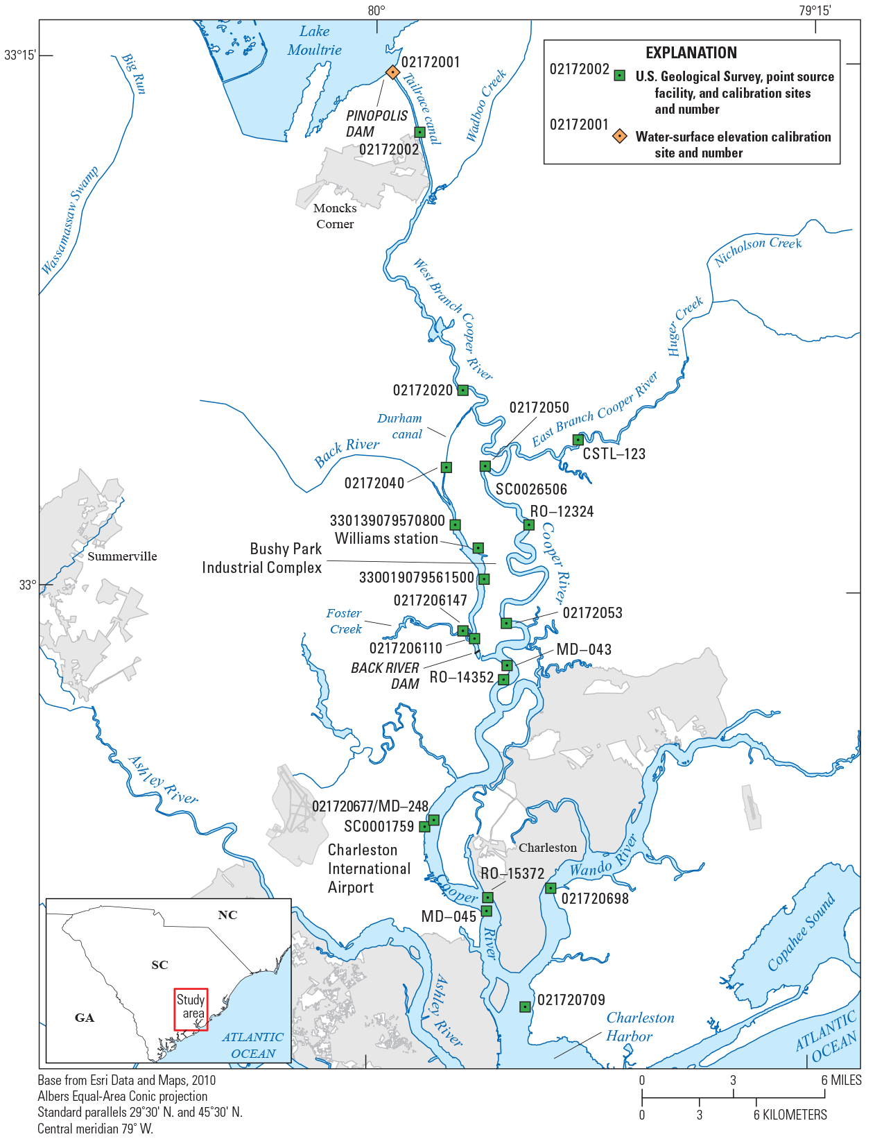
U.S. Geological Survey and point source facilities stations, including calibration sites for water-surface elevation, water temperature, salinity, nutrients, dissolved oxygen, and chlorophyll a.
In addition to the water-temperature records in table 3, four stations were included as calibration targets. USGS stations not included in table 3 (U.S. Geological Survey, 2022) with daily or monthly records included: Bushy Park Reservoir above Foster Creek, Goose Creek, S.C. (USGS station 0217206110); CWS-6 at Foster Creek, Goose Creek, S.C. (USGS station 0217206147); CWS-5 on Bushy Park Reservoir, Goose Creek, S.C. (USGS station 330019079561500); CWS-3 on Bushy Park Reservoir, Goose Creek, S.C. (USGS station 330139079570800). Additionally, SCDHEC stations with monthly records also were included as water-temperature calibration targets (M. Akasapu-Smith, Tetra Tech, unpub. data, 2021; at the time of publication, data were not available from Tetra Tech).
Salinity Boundary Conditions
Every flow series within the EFDC model required a salinity estimate. A constant salinity of 0.07 practical salinity unit (PSU) was assigned to all Bushy Park Reservoir EFDC model-flow time series except for the Pinopolis Dam and the open boundary condition. The basis for 0.07 PSU was determined from 60 salinity records, collected monthly between 1999 and 2002, from 4 SCDHEC stations.
For the Pinopolis Dam, the hourly time series from USGS station 02172020 was applied to the Pinopolis Dam flow-boundary time series (U.S. Geological Survey, 2022). For the open boundary condition, the continuous 30-minute specific-conductance record from USGS station 021720709 (Cooper River at U.S. Highway 17 at Charleston, S.C.) (fig. 4) (U.S. Geological Survey, 2022) was transformed into a continuous salinity record using Schemel’s practical salinity scale equation (Schemel, 2001). With the converted salinity record, the 30-minute record was averaged to an hourly time series for the EFDC model. Additionally, multipliers were applied to the salinity record for each of the six vertical model layers (from top to bottom, layers 1–6): 0.85, 0.90, 0.95, 1.0, 1.05, and 1.05, respectively. These multipliers were added to better represent typical salinity gradients.
In addition to the input salinity series included in the model, additional USGS and SCDHEC stations were used as calibration targets as designated in table 3. These stations mostly included specific-conductance records rather than salinity, so a conversion from specific conductance to salinity was necessary for comparison. USGS stations not included in table 3 (U.S. Geological Survey, 2022) with either daily or monthly records for specific conductance included: Bushy Park Reservoir above Foster Creek, Goose Creek, S.C. (USGS station 0217206110); CWS-6 at Foster Creek, Goose Creek, S.C. (USGS station 0217206147); CWS-5 on Bushy Park Reservoir, Goose Creek, S.C. (USGS station 330019079561500); CWS-3 on Bushy Park Reservoir, Goose Creek, S.C. (USGS station 330139079570800). Additionally, SCDHEC stations with monthly specific-conductance records also were included as calibration targets (M. Akasapu-Smith, Tetra Tech, unpub. data, 2021; at the time of publication, data were not available from Tetra Tech).
Meteorological Data
Meteorological data were required as input to the EFDC model because of the importance of surface-boundary conditions to the overall model performance, specifically surface-heat exchange, solar radiation absorption, wind stress, and gas exchange. Required meteorological data included air temperature, atmospheric pressure, relative humidity, total precipitation, wind speed, wind direction, and cloud cover. All meteorological data input files were developed from the Charleston International Airport (fig. 3) (Weather Bureau Army Navy [WBAN] station identification number 13880; not shown) (National Climatic Data Center, 2017). Solar radiation was calculated using cloud cover data from WBAN 13380 using a Tetra Tech software package, the Meteorological Data Analysis and Preparation Tool (MetADAPT).
Water-Surface Elevations
Water-surface elevations in the Bushy Park Reservoir EFDC model were calibrated based on seven stations located throughout the study area. Most of the seven stations included continuous water-surface elevations for the entire period from 2012 to 2015. The seven stations included the following (fig. 4) (U.S. Geological Survey, 2022): Lake Moultrie near Pinopolis, S.C. (tailrace) (USGS station 02172001); Lake Moultrie Tailrace Canal at Moncks Corner, S.C. (USGS station 02172002); West Branch Cooper River at Pimlico near Moncks Corner, S.C. (USGS station 02172020); Back River at Dupont Intake near Kittredge, S.C. (USGS station 02172040); Cooper River near Goose Creek, S.C. (USGS station 02172050); Cooper River at Mobay near North Charleston, S.C. (USGS station 02172053); and, Cooper River at Filbin Creek at North Charleston, S.C. (USGS station 021720677).
Water Quality
The Bushy Park Reservoir EFDC model-simulated water quality for nutrients (nitrogen and phosphorus), DO, total phytoplankton biomass (represented by one algae group and output as chlorophyll a), and organic carbon. For nutrients, specific classes included ammonia, nitrate, organic nitrogen (divided into refractory particulate organic nitrogen and dissolved organic nitrogen), orthophosphate, and organic phosphorus (divided into refractory particulate organic phosphorus and dissolved organic phosphorus). The water-quality setup for model simulation required inputs for boundary conditions and parameters to control the water-quality module. The basis for the selected water-quality parameters mostly came from the default value used in the original EFDC model (U.S. Army Corps of Engineers, 2015).
Water-quality data selected to specify the boundary conditions for each of the freshwater flow series, such as the Pinopolis Dam, Back River, and Foster Creek, were limited. Data were assembled mostly from outside the model domain but did include two stations on Foster Creek. Much of the other data were assembled from Lake Moultrie (fig. 3). Water-quality data frequency generally were assembled at monthly intervals for the model-simulated time interval. Additionally, no water-quality stations contained all the required input data so multiple datasets had to be combined.
Another challenge for defining the water-quality conditions at the freshwater flow boundaries was obtaining data unaffected by tidal effects. Therefore, another source of water-quality data to define the boundary conditions, in particular, the three synthetic Cooper River tributaries (East Cooper River, Cooper River upstream of the Tee, and the Cooper River middle), was from watershed loads (including non-point and point sources) developed using a multi-variable regression analysis (M. Akasapu-Smith, Tetra Tech, unpub. data, 2021; at the time of publication, data were not available from Tetra Tech). These loads were based upon previous work completed from 2001 to 2003 for the Upper Ashley River watershed, located to the west of the Bushy Park Reservoir EFDC model domain (Cantrell, 2013; fig. 3). The watershed loads calculated from Foster Creek and Back River watersheds entering Bushy Park Reservoir were confirmed to be consistent with the Spreadsheet Tool for Estimating Pollutant Load (STEPL) watershed loads estimated by CWS for the Foster Creek and Back River watersheds.
Other water-quality information necessary for running the model included point source data, derived from 10 different NPDES facilities (not shown on a map). The open boundary water-quality conditions for the southern end of the EFDC model domain were derived from two different SCDHEC stations: Cooper River above mouth of Shipyard Creek at Channel Buoy 49 (SCDHEC station MD-045) and Cooper River 1.6 mi NE of mouth of Shipyard Creek (SCDHEC station RO-15372). Marsh cells used loads derived from the original CHS water-quality model (Cantrell, 2013). Finally, atmospheric inputs were developed from annual deposition data collected at Fort Johnson, in Charleston Harbor, S.C., the same National Atmospheric Deposition Program used in the CHS water-quality model (National Atmospheric Deposition Program, 2022).
Model Parameterization
Selected hydrodynamic model parameters for the Bushy Park Reservoir EFDC model are shown in table 4. Model parameters were varied by trial and error through a series of calibration model runs to improve the overall model fit, often by adjusting one or more model parameters per calibration run to understand the effect on the calibration metrics for water-surface elevations, discharge, and temperature. For an example of a typical calibration effort for an EFDC model, Smith and others (2020) discussed controlled variations in parameter settings across select ranges of parameter values for each calibration run. This effort can often be intensive and requires appreciable time to properly parameterize the model for both the model calibration and general model stability.
Table 4.
Major model parameters important for calibration in the Bushy Park Reservoir model, South Carolina, including the parameter, parameter description, and the final parameter value. For the bottom roughness, the final parameter value includes a range as each grid cell contains a unique value.[m, meter; m/s, meter per second; m2/s, square meter per second; hr, hour; °C, degree Celsius]
Based on other EFDC calibration efforts and model parameterization (Smith and others, 2020; Smith and Shah, 2020), many of the parameters that affect hydrodynamics, such as AVO, ABO, AVMN, and ABMN (table 4), were considered neutral to insensitive in their effects on any of the primary calibration targets: water-surface elevation, discharge, water temperature, and flow velocity. On the other hand, salinity can be sensitive to changes in AVO and ABO. Other parameters, such as bottom roughness coefficient values, can be sensitive. The bottom roughness values across the grid of the Brushy Park Reservoir EFDC model varied in a range from 0.005 to 0.07 meter (m). Bottom roughness values in Bushy Park Reservoir, Foster Creek, Back River and a part of Cooper River were set to 0.005 m, marsh cells set to a range from 0.04 to 0.07 m, and the remainder were set to a range from 0.025 to 0.01 m. Bottom roughness values set the channel friction applied to the flow.
For the water-quality module, many different parameters affect dispersion, DO saturation, reaeration, sediment oxygen demand, nutrients, and total phytoplankton biomass (Hamrick, 1992; 1996). No specific details were given on the parameterization scheme, except that the water-quality parameters were varied by trial and error through a series of calibration model runs to improve the overall model fit and the initial water-quality parameters were largely based on the CHS model (Cantrell, 2013; U.S. Army Corps of Engineers, 2015). These parameters include rates, constants, and kinetics formulations. Although no detailed discussion will be included on the water-quality module here, some specific suggestions for improving the EFDC model for future application, specifically related to taste-and-odor issues will be included later in the “Potential Modifications and Considerations for Model Improvements” section.
Hydrodynamic Model Calibration
The Bushy Park Reservoir EFDC model was calibrated for a period from January 1, 2012, to December 31, 2015. For purposes of carefully examining the model application described here for possible future application, this review focuses on the appropriate use of the model based upon the description, calibration statistics, and figures provided to the USGS (M. Akasapu-Smith, Tetra Tech, unpub. data, 2021; at the time of publication, data were not available from Tetra Tech). Part of the description, in relation to the calibration, will determine if the model, with additional effort, could be developed into an adequate planning tool for the CWS.
As mentioned earlier, four primary statistics were used to evaluate the degree of fit for the EFDC model described in this report, including MAE, RMSE, NRMSE, and the IA. Based on previous USGS calibration efforts, the MAE, RMSE, and NRMSE are common metrics used for model calibration and have been used frequently by the USGS in other model calibrations (for example, Sullivan and Rounds, 2004; Galloway and Green, 2007; Rendon and Lee, 2015). Although these metrics do not directly focus on the model performance, these metrics are appropriate for quantifying the error between the measured and simulated data.
Discharge
The discharge across the model domain was calibrated from January 1, 2012, to December 31, 2015. Continuous measured discharge was compared at two locations: (1) Pinopolis Dam tailrace (USGS station 02172002; table 1, fig. 2); and (2) Durham Canal (USGS station 02172040; table 1, fig. 2). Without a discharge record directly from Pinopolis Dam, this USGS streamgage was also applied as the inflow boundary condition from Lake Moultrie, so the high IA of 0.86 was expected (table 5). However, as the station is approximately 2 mi downstream from Lake Moultrie, differences between the measured and simulated data are present (fig. 5) and can be partially attributed to this offset, although the index of agreement sensitivity to extreme values can sometimes produce high IA values even for less than adequate calibrations (Legates and McCabe, 1999). Ebb flows derived from tidally affected flows were higher in model simulation than measured data. Additionally, both the simulated and measured data illustrate the complicated discharge patterns in the West Branch of the Cooper River, even as far upstream as the Pinopolis Dam tailrace, which is reflective of the Pinopolis Dam releases (fig. 5).
Table 5.
Index of agreement values for discharge, flow velocity, and water-surface elevations of the Bushy Park Reservoir model, South Carolina, 2012–15.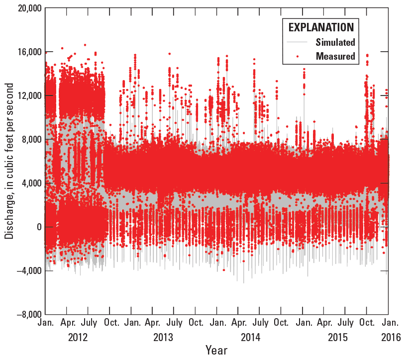
Subhourly measured and simulated discharge for the Lake Moultrie Tailrace Canal at Moncks Corner, South Carolina (U.S. Geological Survey station 02172002), also referred to as the Pinopolis Dam tailrace, from January 1, 2012, to December 31, 2015. Negative discharge values indicate a reversal of flow (ebb flows resulting from tidal effects).
The other streamgage used for model calibration, Durham Canal (USGS station 02172040) (fig. 2), was an important descriptor of model performance because Durham Canal is the largest freshwater exchange to Bushy Park Reservoir, connecting the upper reaches of the Back River and the freshwater reaches of the West Branch of the Cooper River (fig. 6). To accurately simulate the flow dynamics in and out of Bushy Park, the IA of 0.75 verified good agreement between the measured and simulated flow through the Durham Canal (table 5). Tidally filtered discharge data were available from September 13, 2013, through the end of 2015. This period was reasonably long to demonstrate the capacity of the model to adequately characterize flow through the canal. It should be noted that the measured discharge was filtered using a Godin filter (Godin, 1972) to eliminate the effects of tidal aliasing in the continuous time-series discharge. The simulated output was a daily average; therefore, the measured data and simulated results were not entirely exact but were in good agreement with the tidal effects largely removed.

Simulated daily mean discharge for the Back River at Dupont Intake near Kittredge, South Carolina (U.S. Geological Survey station 02172040), compared to the measured discharge filtered with a Godin filter (Godin, 1972) to eliminate the effects of tidal aliasing, from January 1, 2012, to December 31, 2015. Negative discharge values indicate a reversal of flow (ebb flows resulting from tidal effects).
Generally, the other two major water sources to Bushy Park Reservoir, the Back River and Foster Creek, had low discharge rates (less than 100 ft3/s for the Back River and less than 20 ft3/s for Foster Creek) except during major rainfall events (Conrads and others, 2017a). Aside from the Durham Canal, the largest effect on both flow and circulation in Bushy Park Reservoir was the Williams Station. The Williams Station was included as both an intake and discharge in the model domain (table 2).
For improvements to the Bushy Park Reservoir EFDC model, additional flow-calibration stations would be preferable for a domain the size of this model, given that only two streamgages were available within the model domain. Continuous discharge measurements were not available inside of Bushy Park Reservoir boundary; therefore, it was difficult to determine if the simulated flow and circulation patterns were similar to the actual flow patterns. Additionally, the Back River streamgage (USGS station 021720603) and Foster Creek streamgage (USGS station 021720612) were only available for less than 1 year during the calibration period; therefore, continuing operation of these stations would also improve model simulation. Because of the lack of continuous discharge measurements, future Bushy Park Reservoir model runs could include discrete cross-section measurements of discharge and velocity from within Bushy Park Reservoir to help verify that model-simulation results were reasonable.
Flow Velocity
Because the discharge measurements and simulated results are an integration of the flow velocity, the similarity in the predictive success of discharge and velocity in model simulation was expected. The model was able to accurately simulate flow velocity dynamics in and out of Bushy Park Reservoir by way of the Durham Canal, although the amplitude for the simulated flow velocity was larger than the measured flow velocity, particularly with negative flows out of Bushy Park Reservoir through the Durham Canal (USGS station 02172040) (fig. 2). For comparison, the Pinopolis Dam tailrace and Durham Canal were used as calibration datasets: the IA values for Pinopolis Dam tailrace and Durham Canal were 0.82 and 0.73, respectively. Similar to the discharge measurements, other velocity calibration metrics would normally be desirable for a model domain the size of the Bushy Park Reservoir EFDC model. Also, the USGS collected vertical-velocity profile data at 6 locations and tidal-cycle water-velocity transect data at 5 locations between 2013 and 2015, so using these datasets instead of continuous discharge could be beneficial (Conrads and others, 2017a; Conrads and Lanier, 2017).
Water-Surface Elevations
A total of seven USGS streamgages (fig. 4) were available for water-surface elevation comparisons between measured data and simulated values from January 1, 2012, to December 31, 2015. In the absence of more flow velocity and discharge calibration stations, model calibration for water-surface elevation throughout the model domain was the best approximation for determining the overall model fit for hydrodynamics. Throughout the model-simulation period from 2012 to 2015, the general range at all stations (relative to North American Vertical Datum of 1988, in feet) was from −5 to 5 ft, with some periods outside that range. The IA across the seven stations was from 0.74 to 0.99, with stations representing flow elevations across the model domain.
Two examples of the model fit to measured data are shown in figures 7A and 7B. Lake Moultrie tailrace (USGS station 02172002) simulated the general range throughout the model-simulation period (fig. 7A), although the simulated range was higher (overprediction) than the measured water-surface elevation. This overprediction is partially related to poor bathymetric control in this part of the model domain. However, the other possible reason for the model overprediction resulted because of too much tidal energy propagating into some of the upstream reaches of the model domain. Another station, Cooper River at Mobay near Charleston, S.C. (USGS station 02172053), is shown in figure 7B. Water-surface elevations, in good agreement between the simulated and measured values, were simulated for the entire model domain, with an IA for this station of 0.97.
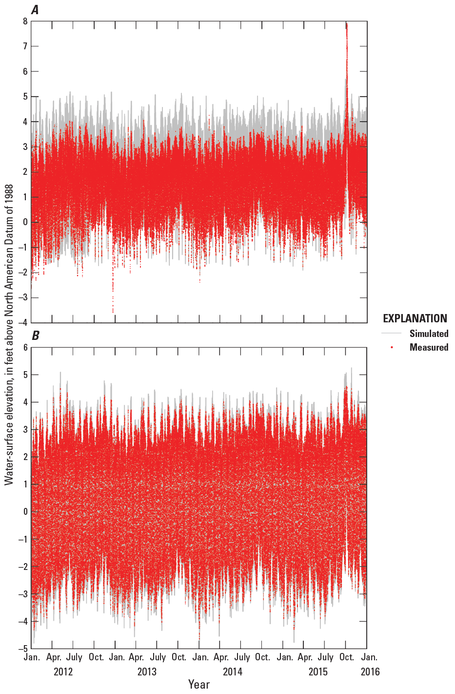
Subhourly water-surface elevations for Bushy Park Reservoir locations, South Carolina. A, Lake Moultrie Tailrace Canal at Moncks Corner, South Carolina (U.S. Geological Survey [USGS] station 02172002), 2012–15. B, Cooper River at Mobay near Charleston, South Carolina (USGS station 02172053), 2012–15.
Water Temperature
Temperature calibration was important in model simulation because temperature affects water density and the vertical exchange of constituents. Temperature also affects all biogeochemical processes within the water column, so the temperature calibration is considered a critical step in water-quality modeling. Four to five boundary conditions affect the water temperature, including the initial water temperature and the sediment temperature exchange; however, the two most important boundary conditions for the Bushy Park Reservoir model are the availability of the inflow temperature records for at least a subset of the flow series and high-resolution meteorological records from near (within 5 mi) to the model domain.
A total of 16 stations were used for at least part of the 4-year simulation period as calibration datasets, 6 that were continuous record stations (table 6). The IA range across all comparisons was from 0.95 to 1.00, demonstrating excellent agreement between the measured and simulated results. MAE and RMSE for the simulations were from 0.54 to 2.94 degrees Fahrenheit for 15 of the 16 stations, and NRMSE of 0.08 or less for all station locations. One station, RO-15372, had only 11 measurements with 1 measurement falling outside the overall seasonal trend, which was possibly an erroneous measurement, such as an equipment issue, causing larger MAE and RMSE values.
Table 6.
Performance evaluation statistics for water temperature and salinity of the Bushy Park Reservoir model, South Carolina, 2012–15, including mean absolute error, root mean square error, normalized root mean square error, and the index of agreement.[PSU, practical salinity unit; MAE, mean absolute error; RMSE, root mean square error; NRMSE, normalized root mean square error, IA, index of agreement; CWS, Charlotte Water System; --, no data]
Aside from simulating the water-temperature dynamics at 16 different locations across the model domain, the general amplitude throughout the year was also accurately simulated with the model. Despite only applying the same aggregated temperature record to all inflow series, the water-temperature dynamics was accurately simulated with the model. An example comparison between measured and simulated water-temperature dynamics is shown in figure 8 for the Cooper River at Mobay near Charleston, S.C. (USGS station 02172053; fig. 4). In the case of the Bushy Park Reservoir EFDC model, the temperature calibration was a good approximation of the continuous measured temperatures at all 16 stations.
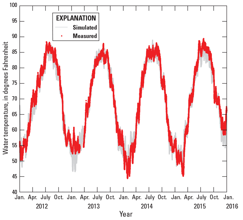
Subhourly water temperature (in degrees Fahrenheit) for the Cooper River at Mobay near Charleston, South Carolina (U.S. Geological Survey station 02172053), 2012–15.
Salinity
The salinity calibration was important to determine the reliability of the salinity model predictions, particularly in Bushy Park Reservoir and Durham Canal. A total of 15 stations were used for calibration, with 5 continuous salinity stations (or converted specific-conductance records) between 2012 and 2015. Of the 15 stations, 5 of the stations were located either within Bushy Park Reservoir or within the tributaries to Bushy Park Reservoir (for example, Foster Creek and Durham Canal (fig. 1).
The quality of model simulations and predictions ranged widely, with an IA from 0.15 to 0.92. Because there was such a wide variety of measured salinity values for the 15 stations, common for an estuarine environment, the MAE and RMSE ranges were large. NRMSE was less than 1.1 for 13 of 15 stations, with only 2 stations above this range with NRMSE values of 3.09 and 8.76. Both stations with high NRMSE values had low IA values, with the lowest IA resulting closest to the boundary condition on the southern end of the model domain. Additionally, some of the stations with lower IA values, such as Cooper River approximately 2.75 mi southeast of the Tee, S.C. (RO-12324) and CWS-3 on Bushy Park Reservoir Goose Creek, S.C. (USGS 330139079570800) with IA values of 0.15 and 0.18, respectively, had a wider range in salinity values with less than 20 measurements.
Overall, the general salinity trends were simulated with the model, particularly for the five stations related to Bushy Park Reservoir. Durham Canal (USGS station 02172040 (fig. 2)) is an important station for model calibration because of its location where exchange between the freshwater reaches of the West Branch of the Cooper River and Bushy Park Reservoir takes place. This station had a continuous record for the entire simulation period with an IA of 0.73 and NRMSE of 0.15. The simulated record was less variable across the entire time from 2012 to 2015 than the measured data; therefore, the model did not accurately simulate some of the larger deviations resulting during individual hydrologic events such as during January 2014 (fig. 9). Therefore, it may be difficult to simulate extreme events, such as large storms, where more saline water is exchanged with freshwater in the Bushy Park Reservoir. General salinity trends and patterns were successfully simulated with the model as indicated with the four stations within the Bush Park Reservoir (table 6). However, the calibration statistics for these stations were not as reliable, as the sparseness of some of these sample records (often less than 15 samples) skewed the final calibration statistics (table 6). This result is a general challenge for discrete calibration records with only limited data points, as the simulated value for an individual grid cell represents a large area, whereas a measured data point is one specific location within the larger grid cell.

Daily measured and simulated salinity (in practical salinity units) for the Back River at Dupont Intake near Kittredge, South Carolina (U.S. Geological Survey station 02172040), also known as the Durham Canal, 2012–15.
It is difficult to ascertain the depth characteristics of simulated salinity values for the Bushy Park Reservoir model, given no continuous calibration records are present with multiple sample depths. For example, the Lake Houston EFDC model (Rendon and Lee, 2015; Smith and Shah, 2020) had continuous measurements for four different depths at two different locations as calibration targets to determine the model capacity to replicate salinity with depth. Whereas this capacity may not be as important for shallow areas, stations with multiple sample depths for deeper locations (such as closer to Charleston Harbor), multiple calibration depths would be beneficial for model simulation. For discrete measurements, multiple USGS station locations within Bushy Park Reservoir did have approximately seven sampling events with multiple depths for either salinity or specific conductivity, but this dataset was not used for model calibration. Likewise, AUV data also were available between 2013 and 2015 (Conrads and others, 2017b); however, they were not used for model calibration during this period (Conrads and others, 2017a).
Other limitations to the modeling framework could be improved for salinity simulation by application of better bathymetry controls, particularly outside areas that included the updated USGS bathymetry. Only the original Post 45 coarse model bathymetry data were used in these areas. For example, updated bathymetry for the West Branch of the Cooper River would possibly improve model-simulated salinity predictions. Inside areas with updated USGS bathymetry, in particular the Bushy Park Reservoir, the average grid cell size could be reduced with minimal computational effort. With higher-quality bathymetry, included in the modeling framework, the model could better simulate the exchange of high saline water from the Atlantic Ocean with the freshwater portions of the West Branch of the Cooper River upstream.
Finally, an improvement in the modeling framework would be the inclusion of more continuous salinity records as either boundary-condition records or calibration targets. The lack of continuous salinity records for Bushy Park Reservoir, for example, makes the calibration for Bushy Park Reservoir appear inaccurate. For example, the USGS stations 330139079570800, 330019079561500, 0217206110, and 0217206147 all had IA values below 0.35 (table 6). The simulated values were near the measured values for the USGS station 330019079561500 (fig. 10), as an example, but there were only 20 data points to compare for the entire simulation period. Also, there was a mixture of sample depths included, some from 3 ft and some from 10 ft; therefore, the comparison of salinity values at a grid level can be problematic if mixing multiple depths when the salinity is vertically stratified (same case for temperature and other water-quality comparisons, such as DO concentration). Future simulation periods with new salinity records may either improve the model calibration, or at least advance new calibration targets for adjusting model parameters. In addition, the application of a constant salinity of 0.07 PSU for most of the inflow boundary conditions limits the effect of boundary conditions on the model domain. However, similar to the calibration targets, the lack of continuous salinity records during the study period (2012–2015) was a limitation in model simulation, but future inclusions of continuous salinity records would likely improve the present modeling framework.
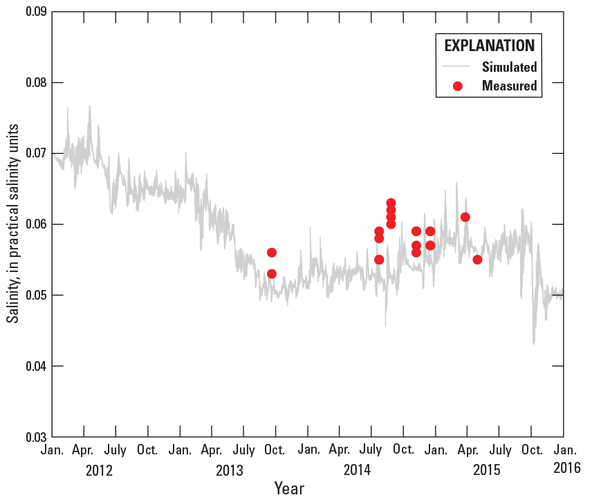
Sub-hourly simulated salinity (in practical salinity units) for the CWS-4 on Bushy Park Reservoir, Goose Creek, South Carolina (U.S. Geological Survey station 330019079561500), compared to 20 measured comparison points for the same location, 2012–15.
Water Quality
An iterative process was used for calibrating water quality, with parameters initially based on an earlier version of the EFDC model (Cantrell, 2013; U.S. Army Corps of Engineers, 2015). The model review described in this report is limited and not comprehensive. Instead, model description was divided between nutrients (nitrogen, phosphorus, and its species), DO, total phytoplankton biomass (represented by one algae group and output as chlorophyll a), and organic carbon, followed by a brief discussion on recommendations for future improvements to the water-quality modules.
Nutrients
The Bushy Park Reservoir EFDC model was calibrated for total nitrogen (TN), ammonia, nitrate, total Kjeldahl nitrogen (TKN), orthophosphate, and total phosphorus (TP). Similar to all other constituents simulated, the primary calibration focus was improving the statistical metrics such as MAE, RMSE, NRME, and IA (table 7). Twelve calibration stations with a monthly data frequency for at least part of the 4-year simulation period (2012–15) were available for model calibration of TN, ammonia, and TP; eight stations were available for calibration of nitrate and TKN, and four stations were available for calibration of orthophosphate.
Table 7.
Performance evaluation statistic ranges for selected water-quality constituents, Bushy Park Reservoir model, South Carolina, 2012–15. Ranges include mean absolute error, root mean square error, normalized root mean square error, and the index of agreement.[MAE, mean absolute error; RMSE, root mean square error; NRMSE, normalized root mean square error, IA, index of agreement]
The IA values for TN were generally low, particularly for the one West Brach of the Cooper River station, with 10 of the 12 stations below 0.60 (range from 0.00 to 0.83) and only two stations with IA values above 0.60 (0.61 and 0.83). Three of the four stations available for Bushy Park Reservoir or Foster Creek had higher IA values (values included 0.29, 0.58, 0.61, and 0.63), with TN values that generally indicated the overall TN trend and mean concentration. All four of these stations were sampled by the USGS (Conrads and others, 2018). Two Bushy Park Reservoir station comparisons (USGS station 0217206147; USGS station 0217206110) between measured data and simulated results illustrate that model simulation adequately approximated total nitrogen for these locations (fig. 11). However, this result also illustrates the general difficulty in calibrating total nitrogen, with a much poorer model-simulated fit for USGS station 330139079570800, also within Bushy Park Reservoir. This station location, not illustrated in this report, had an IA of 0.29 based on only six available measured TN results.
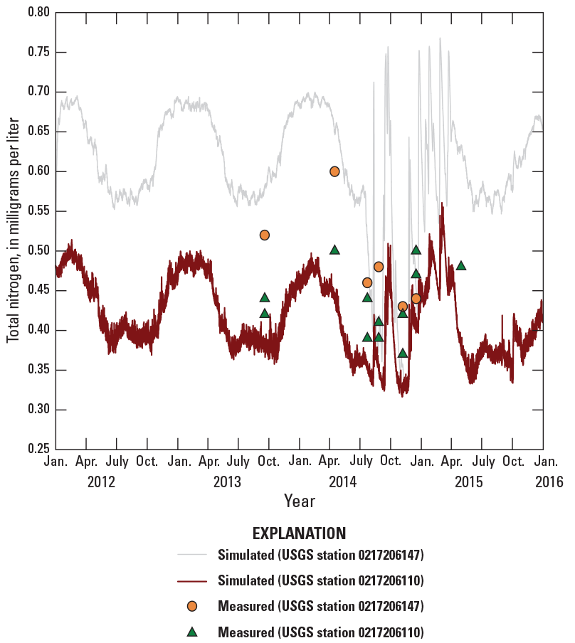
U.S. Geological Survey measured total nitrogen results (in milligrams per liter) for two stations (U.S. Geological Survey [USGS] stations 0217206147 and 0217206110) compared to the continuous total nitrogen simulations for the same locations, Bushy Park Reservoir, South Carolina, 2012–15.
Ammonia was sampled at the same 12 stations as TN with less frequency. Largely, the EFDC model did not simulate ammonia patterns when compared to the measured data collected from these 12 stations. This result is reflected in the low IA values ranging from 0.00 to 0.50, with an IA of 0.30 or less at 11 of the stations. MAE and RMSE were generally less than 0.10 for ammonia, but the overall concentrations across the model domain for ammonia were low for both measured and simulated ammonia concentrations. It should be noted that some of the low IA values were from stations with six or less samples.
Nitrate and TKN were sampled at eight stations, and similar to ammonia, the model did not accurately simulate the measured data. Whereas the overall average for most stations used for nitrate and TKN calibration was similar to the measured data, the measured data included more scatter than the model-simulated results. For nitrate, IA values ranged from 0.00 to 0.55. The nitrate MAE and RMSE range was from 0.02 to 0.12 with one outlier of 0.75 and 2.06 for MAE and RMSE, respectively, at a station on West Branch of Cooper River. TKN had an even lower IA range from 0.01 to 0.32. For both nitrate and TKN, the measured data frequency was low, and none of the eight stations sampled for nitrate were located within the Bushy Park Reservoir.
TP was sampled at the same 12 stations as TN and ammonia, whereas orthophosphate data was only available for 4 stations. Similar to the nitrogen species, such as ammonia and nitrate, phosphorus concentrations were not simulated accurately with the model. IA ranged from 0.02 to 0.49 for the 12 TP stations, whereas IA ranged from 0.29 to 0.60 for orthophosphate. Unlike the other constituents, the model did at least simulate the general trends of the orthophosphate data (not shown) for the time periods data were available, primarily from September 2013 to early 2015, overlapping with the time frame the USGS sampled the Bushy Park Reservoir sites (Conrads and others, 2018). This period also overlapped with the periods where the USGS was collecting continuous discharge data for both the Back River and Foster Creek streamgages (table 1).
Most of the limitation for simulating nutrients across the model domain was the lack of characterization for the incoming constituents, such as characterizing the loads from Foster Creek and the Back River to Bush Park Reservoir. In many other hydrodynamic and water-quality models, constituent loads are simulated to better understand the nutrient fluxes into the particular model domain. For example, Smith and others (2018) calculated continuous loads using the LOADEST program (Runkel and others, 2004) for all incoming flow series to Lake St. Croix in Wisconsin and Minnesota. In order to prescribe water-quality loads to Bushy Park Reservoir, the stations need to be located outside Bushy Park Reservoir but on tributaries discharging to the reservoir or on the Cooper River. One exception was the inclusion of Upper Ashley River locations to help define the watershed loads derived for the Cooper River. Whereas similar nutrient trends could be expected from regional streams, the lack of boundary-condition data for the present Bushy Park Reservoir EFDC model domain is a limitation to the current model framework.
Dissolved Oxygen
Within the Bushy Park Reservoir EFDC model, many sources and sinks are present; this makes DO one of the more difficult constituents to accurately simulate (Hamrick, 1992; 1996). Eleven stations were available for DO calibration, including four stations either in Bushy Park Reservoir or on Foster Creek. Most of the stations only included monthly measurements, with a subset of stations that included measurements for all 4 years of the calibration period (2012–15).
The IA for all 11 stations ranged from 0.58 to 0.94, with NRMSE values from 0.11 to 0.37. For the four stations associated with Bushy Park Reservoir, the IA ranged from 0.58 to 0.66. Considering the difficulty of DO model calibration, DO trends (not shown) were adequately characterized in the EFDC model. DO generally followed a predictable pattern for both the measured and simulated data, with the highest measured and simulated DO concentration values in the winter months, and the lowest values in the summer months.
Future modeling efforts would benefit from at least one continuous-monitoring station located in Bushy Park Reservoir to characterize not only seasonal trends, but to better understand daily DO concentration variations. DO dynamics are directly tied to phytoplankton production, including cyanobacteria, and other trophic dynamics that can be simulated with the EFDC water-quality modules. Therefore, the availability of a continuous DO record could help refine diurnal dynamics. Without a continuous station for assessing Bushy Park Reservoir, it is difficult to determine whether the DO trends would be applicable during a discrete event, such as storm surge through the Durham Canal or the Back River Dam overtopping. Currently (2022), continuous DO monitoring is available for USGS station 02172002 (Pinopolis Dam tailrace) (fig. 2) but this station only became available in 2016 and would not help determine DO trends directly in Bushy Park Reservoir.
Chlorophyll a
Seven stations were included for chlorophyll a, including four stations either directly from Bushy Park Reservoir or near (indirectly from) Bushy Park Reservoir on Foster Creek. The mean chlorophyll a measured concentration ranged from 2.88 to 9.25 micrograms per liter (μg/L), for the seven stations with a mean simulated concentration range from 1.51 to 4.80 μg/L. For most stations, model simulations resulted in lower chlorophyll a concentration values (underpredicted) than measured values collected from the seven stations. The IA across the seven stations had a range from 0.11 to 0.74, although the highest of 0.74 was based on only five measurements. For the four Bushy Park Reservoir stations, the IA had a range from 0.25 to 0.54. Most of the simulated values were close to the measured values, although there were typically one or two measurements that were appreciably different from simulated values. For example, CWS-6 at Foster Creek, Goose Creek, S.C. (USGS station 0217206147) was close for six of the seven measurements but one measured value was much higher that caused the IA value to be low (0.25) (fig. 12).
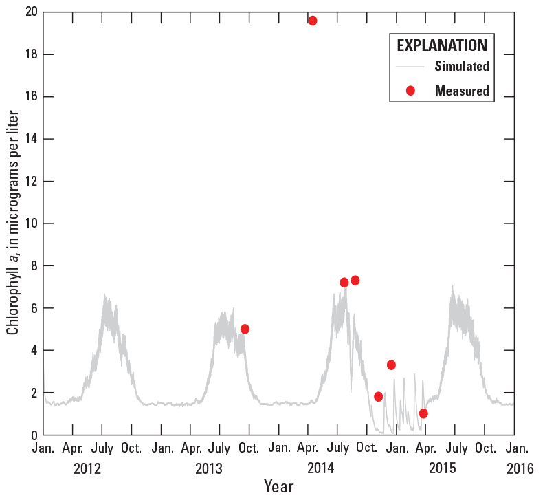
U.S. Geological Survey measured total chlorophyll a (in micrograms per liter) for CWS-6 at Foster Creek, Goose Creek, South Carolina (U.S. Geological Survey station 0217206147) compared to the continuous chlorophyll a simulation results for the same location, 2012–15.
Overall, for a better chlorophyll a model calibration, continuous records would be beneficial to determine if the model accurately simulated both seasonal trends and if the model can specifically simulate individual bloom events. Because no continuous record was available for the model-calibration period (2012–15) chlorophyll a could not be calibrated. However, the USGS did acquire continuous AUV measurements of chlorophyll a from approximately 17 surveys between September 2013 and April 2015. The AUV dataset could be used to assess the calibration fit for chlorophyll a across specific transects within the modeling framework. Otherwise, the calibration is limited considering most stations had less than 10 individual chlorophyll a measurements from 2012 to 2015.
Algae
In general, taste-and-odor events in reservoirs, such as Bushy Park Reservoir, are related to the production of geosmin and MIB. Both compounds are metabolites usually produced by cyanobacteria (Graham and others, 2018). As mentioned earlier, geosmin and MIB both frequently are present in Bushy Park Reservoir (Conrads and others, 2018). Whereas it is difficult for hydrodynamic and water-quality models, such as the Bushy Park Reservoir EFDC, to directly simulate these compounds, positive correlations of metabolites could be related to cyanobacteria biomass in the modeling framework because it is likely higher cyanobacteria biomass would lead to higher number and concentrations of metabolites. The EFDC model has the capacity to simulate up to three algae groups (diatoms, cyanobacteria, and green algae). However, an accurate model representation of the different algae groups requires a detailed assessment of biomass concentrations (typically expressed in units of micrograms per liter) entering the model boundaries, and detailed stoichiometric characterization of algae composition for each phytoplankton group (for example, nitrogen-carbon, phosphorus-carbon, phytoplankton chlorophyll a-carbon ratios).
Detailed phytoplankton group biomass concentrations are not available for the Bushy Park Reservoir and its tributaries, although phytoplankton group biovolume data are available from 2012 to 2015. At least 16 stations affected directly or indirectly to Bushy Park Reservoir were sampled for cyanobacteria within the model-simulation period (Conrads and others, 2018). For each sampling event, the average diatom biovolume concentrations ranged from 20 to 60 percent of the total algae biovolume, green algae ranged from 4 to 23 percent, and cyanobacteria ranged from 1 to 15 percent. Other groups, such as euglenoids, dinoflagelates, yellow-green algae and golden-brown algae, typically accounted from approximately 4 to 11 percent of the total algae biovolume. Individual measurements indicated appreciably more spatial and temporal variability in the algae composition with diatoms varying between 1 to 73 percent, green algae between 0.8 to 49.2 percent, and cyanobacteria between 0.1 to 32 percent.
Whereas the model did accurately simulate total phytoplankton biomass, represented by one algae group and output as chlorophyll a, the model did not accurately simulate the three frequently observed phytoplankton groups of diatoms, cyanobacteria, and green algae (Conrads and others, 2017b; Conrads and others, 2018). Because cyanobacteria was not simulated, the model is limited in its current state to assess cyanobacteria blooms that could be related to taste-and-odor episodes in the Bushy Park Reservoir. Ideally, for the Bushy Park Reservoir modeling framework to be applied for taste-and-odor issues, more focus would need to be placed on model calibration for algal dynamics, specifically for cyanobacteria. Cyanobacteria would need to be simulated, and then new model-calibration efforts would be necessary for adding this group for simulation. However, the available Bushy Park Reservoir biovolume data and model outputs could be used to estimate potential algae group concentrations under certain modeling assumptions. For example, the model-simulated total phytoplankton biomass outputs could be multiplied by the observed ratios between cyanobacteria biovolume and total algae biovolume to estimate cyanobacteria concentrations assuming a 1:1 relation between biovolume and biomass concentrations. The above approach would provide an estimate of cyanobacteria biomass that could be used to support other studies relating cyanobacteria biomass with toxins and odor.
Organic Carbon
No calibration was completed for any organic carbon constituents, including dissolved organic carbon or particulate organic carbon, as this calibration process was not outlined in the statement of work between Tetra Tech and CWS. Furthermore, no split between refractory or labile fractions was included for the particulate organic carbon. However, because settling of particulate matter still affects the water quality in the water column, total refractory organic matter was represented as particulate organic matter to be able to simulate sediment settling. It should be noted that sample data are available for both dissolved organic carbon and total organic carbon for several stations within the Bushy Park Reservoir modeling domain, so further calibration could be possible for organic carbon (Conrads and others, 2018).
Potential Modifications and Considerations for Model Improvements
In general, for hydrodynamic and water-quality models, if the physical processes are sufficiently well characterized, it is possible to accurately resolve the water circulation with proper boundary conditions and sufficient spatial and temporal resolution. Any errors in model results are either a result of the inputs to the model (boundary conditions or model parameters) or because of some intrinsic problems in the model setup or conceptualization (for example, grid resolution, bathymetry, numerical hydrodynamic errors). Much of the model limitations presented thus far considered limitations in the boundary conditions, although it is also important to consider potential model grid limitations and the circulation of water throughout the entire model domain. Calibration statistics can support evaluation of any hydrodynamic model, but goodness-of-fit measures such as the index of agreement (IA) that overcome the shortfalls of correlation-based measures can still be sensitive to extreme values (Legates and McCabe, 1999). For example, the discrepancies between the simulated and measured discharge values for USGS station 02172002 (fig. 5) were explored further in a scatterplot of these datasets (not shown) and confirmed that the high IA value was not an accurate calibration measure. Furthermore, improvements in boundary conditions alone may not solve all the potential model limitations, so it is important to consider and possibly perform sensitivity analysis to make certain that the model setup (for example, grid resolution, bottom roughness coefficients) is not the cause of large output errors. Generally, sensitivity analysis increases or decreases individual boundary conditions in a systemic way to better understand the overall effects on the simulated results. A full sensitivity analysis can not only assist in determining potential issues with boundary conditions, but also in determining limitations in the model domain, such as where boundary-condition changes may have too large or too small of an effect on a specific portion of the model domain.
An example of a possible intrinsic problem with the model setup is the possible indication that excessive tidal energy is being propagated into some of the upstream reaches of the Bushy Park Reservoir system, for example, the large range in simulated water-surface elevations at the Lake Moultrie tailrace (fig. 7A) or more simulated ebb flow values (negative values) at the same location than measured values. In addition, mismatches across various locations between simulated and measured salinity values could be indicative of tidal energy not being distributed properly throughout the model domain. A simple spatial analysis of the simulated salinity errors did not show an overall pattern across the 15 available salinity stations (table 6), although there is a possible bias in salinity values because only limited measurements were available at stations where discrete measurements were collected rather than continuous data collection (table 6).
As discussed previously, taste-and-odor issues in Bushy Park Reservoir are likely related to cyanobacteria blooms. To simulate the presence of cyanobacteria within the Bushy Park Reservoir, the cyanobacteria group would need to be activated for the water-quality module. As cyanobacteria data are present from 2012 to 2015 (Conrads and others, 2018), the same model-simulation period could be used for this calibration, although with potentially limited success given there are limited tributary algal load data into Bushy Park Reservoir available for this period. Whereas the model would not explicitly simulate geosmin and MIB, the capacity to simulate cyanobacteria blooms within Bushy Park Reservoir could help with projecting the effects of possible alternative reservoir operations than current operations.
It should be noted that spatiotemporal changes in the cyanobacteria biomass distribution also would depend on other physical and chemical characterizations (not currently available) that govern the internal cycling, production, and decay of the entire algae community. Examples include the algae-specific cell stoichiometry and nutrient cell requirements for cyanobacteria and other algae groups, nutrient competition by the different algae groups, and differences in algae group growth and death rates. Furthermore, algae biomass measurements would be ideally collected for both the Bushy Park Reservoir and all the tributary entry points to support a comprehensive model setup and calibration.
In addition to activating the cyanobacteria group, the underlying nutrient calibrations would need to be improved. Algal growth is dependent on nutrient and carbon dynamics; therefore, a poor calibration for groups, such as orthophosphate, ammonia, nitrate, total phosphorus, and dissolved plus total organic carbon, would negatively affect simulated algal growth. One possible suggestion for improving the water-quality calibration, particularly for Bushy Park Reservoir, would be to use nutrient loads derived for at least one of the freshwater sources to the reservoir, if not both, of the tributary sources. In the current model setup, water-quality concentrations were used from data collected at stations located on Foster Creek (including USGS station 0217206147 and two other non-USGS stations). Discrete water-quality data for most of the necessary inputs to the EFDC model were also available from 2012 to 2015 at the Foster Creek streamgage (USGS station 021720612) (fig. 4), but not included in the model setup.
Previous USGS hydrodynamic and water-quality models (for example, Smith and others, 2014; Smith and others, 2018) used the load estimator (LOADEST) computer program (Runkel and others, 2004) to estimate daily nutrient loads from available water-quality samples and continuous discharge records. Although the available Foster Creek continuous discharge period was only 9 months, some consideration of the available water-quality data and continuous discharge record could be given in an attempt to create loads or at least create linear interpolations between discrete water-quality estimates. Additionally, the three synthetic Cooper River inputs were defined by loads from the 2001–03 Upper Ashley River watershed study, as explained in the “Water Quality” methods section above. The water-quality module would likely be improved if future water-quality data collected for any of the Cooper River tributaries could then be used to create loads for the model-boundary conditions along the Cooper River.
For additional discharge locations, complete flow records would be ideal for Foster Creek and the Back River than other locations for better characterizing loads and better understanding the water balance for Bushy Park Reservoir. Part of the reason these records were limited was the difficulty in finding suitable streamgaging locations for both tributaries. Because of heavy macrophyte growth, it was often difficult to obtain good acoustic Doppler current profiler (ADCP) measurement for flow velocities (U.S. Geological Survey, 2021), particularly for Foster Creek (T. Lanier, U.S. Geological Survey, oral commun., May 6, 2021). Future locations would need to be carefully scouted, with more frequent visits to keep the streamgaging locations clear of heavy plant growth to maintain a sandy channel bottom. Outside of the Bushy Park Reservoir, an additional discharge station located along the West Branch of the Cooper River would be preferable for model calibration rather than only USGS station 02172002, given its proximity to the boundary condition.
Reservoir Operation Scenarios
In addition to calibrating the Bushy Park Reservoir EFDC model based on data collected from January 1, 2012, through December 31, 2015, three different alternative reservoir operation scenarios were run with the calibrated model (M. Akasapu-Smith, Tetra Tech, unpub. data, 2021; at the time of publication, data were not available from Tetra Tech). The following three model scenarios were developed between CWS and Tetra Tech: (1) reduced withdrawals from one of the large intake-discharge locations for Bushy Park Reservoir, the Williams Station; (2) saltwater intrusion from the ocean through Durham Canal into Bushy Park Reservoir; (3) dam overtopping for the Back River Dam at the southernmost end of Bushy Park Reservoir. The following discussion is limited to the main conclusions of those scenarios.
Reduced Withdrawals for the Williams Station
Any proposed changes in the amount of water withdrawn by the Dominion Energy Williams Station, formerly owned and operated by South Carolina Electric and Gas Company, could potentially have a large effect on flow and water quality. For example, one possible future scenario is up to a 90-percent reduction in water withdrawal by the plant because of changes in the internal cooling system from an open loop to a closed loop. Other possible reductions could eventually result because of possibly converting from a coal-fired plant to a natural gas-sourced plant. This possible conversion has been proposed by Dominion Energy, the parent company of the plant (Johnson, 2021).
To explore the possible changes in flow circulation and water quality for Bushy Park Reservoir, one of the three scenarios included a 90-percent reduction in the amount of water withdrawn from the William Power Station intake during the entire model-simulation period from January 1, 2012, to December 31, 2015. Comparisons were then made for flow (discharge) at four station locations within the Bushy Park Reservoir, one at the Durham Canal, and another at the plant-discharge location, in addition to comparisons for salinity, DO, TN, and TP.
The largest change in flow resulted near the Williams Station intake, a conclusion that was expected given the appreciable withdrawal reduction. The next largest flow change resulted in more appreciable flows at the southern end of Bushy Park Reservoir, and a net increase in flow out of the Bushy Park Reservoir to the Cooper River by way of the Durham Canal (fig. 1). The lack of water usage by Williams Station would result in less water drawn into the reservoir by way of the Durham Canal.
The effect on water quality, resulting from the first scenario described above (decrease in withdrawals at Williams Station), was small concerning salinity, with larger increases for DO concentrations at 4 monitoring stations in Bushy Park Reservoir. The possible increase in DO was attributed to net increases in water depths, causing changes in sediment oxygen demand. Another possible reason for changes in DO concentrations could be the overall increases in retention time, likely increasing the amount of time to support increased phytoplankton growth in the reservoir. Total nitrogen generally decreased across the reservoir, whereas TP generally increased, relative to the baseline (background) scenario. However, without a robust model calibration of water quality given the generally low IA values for both TN and TP, it is difficult to draw strong conclusions concerning the water-quality changes in the reservoir. Simulated algal growth rates are highly affected by nutrients, making it difficult to determine the actual cause(s) of simulated DO changes without a good model fit for nutrients. DO is also highly affected by other processes, such as rates of dissolved organic matter decay, nitrification, and sediment oxygen demand (Wetzel, 2001).
Saltwater Intrusion by way of the Durham Canal
The first of two scenarios to explore saltwater intrusion into Bushy Park Reservoir involved saltwater intrusion by way of the Durham Canal. For this scenario, two large storms over the Charleston area (Hurricane Matthew on October 8–9, 2016, and Hurricane Irma on September 10–11, 2017) were simulated. Both storms occurred outside the model-simulation period, so these storms were simulated separately with base model conditions but simulated for the same specific dates in 2014 (Hurricane Matthew) and for the same specific dates in 2015 (Hurricane Irma). In both cases, model simulations were completed with and without the withdrawal for the Williams Station plant.
For both large storm events described above, the water in the reservoir generally dropped in salinity during the event and in the subsequent days and weeks after the event. The relative amount of salinity decrease varied by station, but the overall salinity decrease reflect the high correlation between the freshwater volume in the reservoir from the precipitation totals and the saline-water circulation within the reservoir. The full recovery time (return to baseline (background) conditions) for both storm scenarios (Hurricanes Matthew and Irma) varied from 2 weeks up to 3 months, although the actual time could vary considerably depending on the actual storm trajectory, the length of the storm over the area, and the total amount of precipitation.
Back River Dam Overtopping
The second of two scenarios to explore saltwater intrusion into Bushy Park Reservoir involved the overtopping of Back River Dam. For this scenario, the model simulated a large storm tide of 12 ft (relative to North American Vertical Datum of 1988) at the offshore EFDC model domain boundary that resulted in up to 1.3 ft overtopping at the Back River Dam. For context, the typical tidal range for the Back River and Foster Creek are between 1.7 and 2.0 ft (Conrads and others, 2017a). Similar to the saltwater intrusion scenario, the focus of this scenario was mostly on salinity concentrations and overall flow patterns in the Bushy Park Reservoir.
In the case of dam overtopping, salinity would immediately rise, with larger increases at the southern end of Bushy Park Reservoir and smaller increases farther up the reservoir. Furthermore, the large event also would cause slight increases of saltwater intrusion by way of the Durham Canal from the West Branch of the Cooper River (farther upstream) (fig. 1), although the dam overtopping by way of the main branch of the Cooper River far exceeded any salinity increases by way of the Durham Canal. The largest salinity increases resulted at the southern end of the reservoir (up to a 1.27 PSU) and at the Amoco Intake (2.56 PSU). After the end of the event that lasted approximately 2 hours, the increases in salinity values at the various stations would drastically decrease over the next 2 weeks, and then slowly decrease back to the baseline salinity values within 3 months.
Summary
The Bushy Park Reservoir is a relatively shallow impoundment in a semi-tropical climate and is the principal water supply for the city of Charleston, South Carolina, and the surrounding areas including the Bushy Park Industrial Complex. Although there is an adequate supply of freshwater in the reservoir, concerns are present over taste-and-odor and saltwater intrusion issues. From 2013 to 2015, the U.S. Geological Survey (USGS), in cooperation with the Charleston Water System (CWS) engaged in a multi-year study of the hydrology and hydrodynamics of Bushy Park Reservoir to better understand factors affecting water-quality conditions in the reservoir. As part of this study, the CWS worked with Tetra Tech, Inc. to develop a Bushy Park Reservoir hydrodynamic and water-quality modeling framework, developed upon earlier efforts by both Tetra Tech and the U.S. Army Corps of Engineers. At the completion of the new modeling framework, the USGS was requested to evaluate the hydrodynamic and water-quality model.
The Bushy Park Reservoir Environmental Fluid Dynamics Code (EFDC) model was calibrated from January 1, 2012, to December 31, 2015, with four primary statistics used by the USGS to evaluate the model calibration, including the mean absolute error, root mean square error, normalized root mean square error, and the index of agreement. The general modeling approach for the newly revised modeling framework was developed with EFDC, a grid-based surface-water modeling package that can simulate three-dimensional flow, transport, and water quality in surface-water systems. This report describes the appropriateness of the Bushy Park Reservoir EFDC model, developed by Tetra Tech, to simulate water discharge, water circulation, surface elevations, temperature, salinity, and other water-quality parameters.
Specifically, the model review focused on the following criteria: (1) determine if the model, with additional effort, could be developed into an adequate planning tool for Bushy Park Reservoir; (2) assess the capacity of the model to specifically address the water quality in the reservoir in relation to taste-and-odor issues and saltwater intrusions; and, (3) evaluate three preliminary water-management scenarios related to reduced withdrawals in the reservoir and saltwater intrusion. The work presented here is limited to performing model simulations to determine the general model stability and model-simulation runtime. A detailed description of the model designs was beyond the scope of this work. Additional information concerning model design can be obtained from the CWS.
Overall, the model was able to simulate discharge, flow velocity, and water-surface elevations with generally good agreement between the simulated and measured values. Specifically, the model was able to accurately simulate discharge at two USGS continuous discharge locations (USGS station 02172002; USGS station 02172040), with index of agreements of 0.86 and 0.75, respectively. A total of seven USGS streamgages, located on the West Branch of the Cooper River, the Durham Canal, and the Cooper River, were available to obtain water-surface elevations, with consistently high index of agreements ranging from 0.74 to 0.99. However, the model did overpredict the simulated water-surface elevation ranges (simulated elevation ranges higher than measured elevation ranges) for two locations near Pinopolis Dam, a location farthest upstream on the West Branch of the Cooper River, possibly indicative of too much tidal energy propagated through the Bushy Park Reservoir EFDC model domain.
For water temperature, a total of 16 stations were available for comparing measured and simulated data for part of the 4-year model-simulation period. The index of agreement range for temperature comparisons was from 0.95 to 0.99, indicating excellent agreement between the measured data and simulated results. One of the primary future applications for the Bushy Park Reservoir EFDC model is to determine the extent of saltwater intrusions throughout the reservoir and surface-water system. The model had a wide range in the quality of salinity prediction, ranging from an index of agreement from 0.15 at Cooper River approximately 2.75 mi southeast of the Tee, S.C., to 0.92 at West Branch Cooper River near Moncks Corner, S.C. Durham Canal, an important calibration location because of its exchange of water between the freshwater reaches of the West Branch of the Cooper River and Bushy Park Reservoir, had a continuous salinity record for the entire simulation period with an index of agreement of 0.73. Although the model did not simulate some of the larger deviations resulting during individual hydrologic events, the seasonal salinity trends were accurately simulated with the model from 2012 to 2015. Therefore, it may be difficult to accurately simulate extreme hydrologic events that exchange higher salinity water with Bushy Park Reservoir, such as during large storms. Model-simulation output results seemed to agree with the measured data either on the quantitative index of agreement values or qualitative agreement in the seasonal salinity data trends.
For water quality, the index of agreement values were generally low for total nitrogen, ammonia, nitrate, total Kjeldahl nitrogen, total phosphorus, and orthophosphate. A total of four stations within Bushy Park Reservoir (two within the reservoir, one Back River station, and one Foster Creek station) were compared to the simulated results. Although water-quality trends were accurately simulated at some specific stations, particularly for Bushy Park Reservoir, the model fit was low for all water-quality constituents at all stations with index of agreements often below 0.50. A limitation for simulating nutrients across the model domain was the lack of characterizing the incoming constituents directly into Bushy Park Reservoir, or the lack of data directly attributed to the boundary condition (for example, the Cooper River). One possible EFDC model improvement would be to use Foster Creek-derived nutrient loads, one of the freshwater sources to the reservoir, as discrete water-quality data were collected for Foster Creek from 2012 to 2015.
References Cited
Blumberg, A.F., and Mellor, G.L., 1987, A description of a three-dimensional coastal ocean circulation model, in Heaps, N.S., ed., Three-dimensional coastal ocean models: Washington, D.C., American Geophysical Union, p. 1–16. [Also available at https://agupubs.onlinelibrary.wiley.com/doi/book/10.1029/CO004.]
Bower, D.E., Sanders, C.L., Jr., and Conrads, P.A., 1993, Retention time simulation for Bushy Park Reservoir near Charleston, South Carolina: U.S. Geological Survey Water-Resources Investigations Report 93–4079, 47 p. [Also available at https://pubs.usgs.gov/wri/1993/4079/report.pdf.]
Camacho, R.A., Martin, J.L., Watson, B., Paul, M.J., Zheng, L., and Stribling, J.B., 2015, Modeling the factors controlling phytoplankton in the St. Louis Bay Estuary, Mississippi and evaluating estuarine responses to nutrient load modifications: Journal of Environmental Engineering, v. 141, no. 3, 16 p., accessed December 28, 2021, at https://doi.org/10.1061/(ASCE)EE.1943-7870.0000892.
Campbell, T.R., and Bower, D.E., 1996, Water quality, bed-sediment quality, and simulation of potential contaminant transport in Foster Creek, Berkeley County, South Carolina, 1991–93: U.S. Geological Survey Water-Resources Investigations Report 95–4247, 135 p. [Also available at https://doi.org/10.3133/wri954247.]
Cantrell, W., 2013, Total maximum daily load revision—Charleston Harbor, Cooper, Ashley, and Wando Rivers: South Carolina Department of Health and Environmental Control Bureau of Water Technical Document Number 0506-13, 31 p., 1 app., accessed December 28, 2021, at https://scdhec.gov/sites/default/files/docs/HomeAndEnvironment/Docs/Chas_Hbr_DO_TMDL.pdf.
Conrads, P.A., and Smith, P.A., 1997, Simulation of temperature, nutrients, biochemical oxygen demand, and dissolved oxygen in the Cooper and Wando Rivers near Charleston, South Carolina, 1992–95: U.S. Geological Survey Water-Resources Investigation Report 97–4151, 58 p. [Also available at https://doi.org/10.3133/wri974151.]
Conrads, P.A., and Lanier, T.H., 2017, Hydrodynamic data of Bushy Park Reservoir, South Carolina 2013–15: U.S. Geological Survey data release, accessed September 8, 2022, at https://doi.org/10.5066/F7GB2274.
Conrads, P.A., Petkewich, M.D., Falls, W.F., and Lanier, T.H., 2017a, Hydrologic characterization of Bushy Park Reservoir, South Carolina, 2013–15: U.S. Geological Survey Scientific Investigations Report 2017–5050, 83 p., accessed December 28, 2021, at https://doi.org/10.3133/sir20175050.
Conrads, P.A., Journey, C.A., Lanier, T.H., Petkewich, M.D., Clark, J.M., and Bradley, P.M., 2017b, Water quality data for Bushy Park Reservoir, South Carolina 2013–2015: U.S. Geological Survey data release, accessed September 8, 2022, at https://doi.org/10.5066/F7NG4NVX.
Conrads, P.A., Journey, C.A., Petkewich, M.D., Lanier, T.H., and Clark, J.M., 2018, Characterization of water quality in Bushy Park Reservoir, South Carolina, 2013–15: U.S. Geological Survey Scientific Investigations Report 2018–5010, 175 p., accessed December 28, 2021, at https://doi.org/10.3133/sir20185010.
Downing, J.A., Watson, S.B., and McCauley, E., 2001, Predicting cyanobacteria dominance in lakes: Canadian Journal of Fisheries and Aquatic Sciences, v. 58, no. 10, p. 1905–1908. [Also available at https://doi.org/10.1139/f01-143.]
Dzialowski, A.R., Smith, V.H., Huggins, D.G., deNoyelles, F., Lim, N.C., Baker, D.S., and Beury, J.H., 2009, Development of predictive models for geosmin-related taste and odor in Kansas, USA, drinking water reservoirs: Water Research, v. 43, no. 11, p. 2829–2840. [Also available at https://doi.org/10.1016/j.watres.2009.04.001.]
Elçi, S., Work, P.A., and Hayter, E.J., 2007, Influence of stratification and shoreline erosion on reservoir sedimentation patterns: Journal of Hydraulic Engineering (New York, N.Y.), v. 133, no. 3, p. 255–266. [Also available at https://doi.org/10.1061/(ASCE)0733-9429(2007)133:3(255).]
Galloway, J.M., and Green, W.R., 2007, Application of a two-dimensional reservoir water-quality model of Beaver Lake, Arkansas, for the evaluation of simulated changes in input water quality, 2001–2003: U.S. Geological Survey Scientific Investigations Report 2006–5302, 39 p. [Also available at https://pubs.usgs.gov/sir/2006/5302/.]
Graham, J.L., Foster, G.M., Williams, T.J., Mahoney, M.D., May, M.R., and Loftin, K.A., 2018, Water-quality conditions with an emphasis on cyanobacteria and associated toxins and taste-and-odor compounds in the Kansas River, Kansas, July 2012 through September 2016: U.S. Geological Survey Scientific Investigations Report 2018–5089, 55 p. [Also available at https://doi.org/10.3133/sir20185089.]
Hamrick, J.M., 1992, A three-dimensional Environmental Fluid Dynamics Computer Code—Theoretical and computational aspects: Virginia Institute of Marine Science, College of William and Mary, Applied Marine Science and Ocean Engineering (SRAMSOE) no. 317, 63 p. [Also available at https://scholarworks.wm.edu/reports/715/.]
Hamrick, J.M., 1996, User's manual for the Environmental Fluid Dynamics Computer Code: Virginia Institute of Marine Science, College of William and Mary, Applied Marine Science and Ocean Engineering (SRAMSOE) no. 331, 223 p. [Also available at https://doi.org/10.21220/V5M74W.]
Hughes, W.B., Abrahamsen, T.A., Maluk, T.L., Reuber, E.J., and Wilhelm, L.J., 2000, Water Quality in the Santee River Basin and coastal drainages, North and South Carolina, 1995–98: U.S. Geological Survey Circular 1206, 32 p., accessed December 28, 2021, at https://doi.org/10.3133/cir1206.
Ji, Z.-G., 2017, Hydrodynamics and water quality—Modeling rivers, lakes, and estuaries 2nd ed.: Hoboken, N.J., John Wiley and Sons, 617 p., accessed December 28, 2021, at https://doi.org/10.1002/9781119371946.
Ji, Z.-G., Morton, M.R., and Hamrick, J.H., 2004, Modeling hydrodynamic and water quality processes in a reservoir, in Spaulding, M.L., ed., Proceedings of the 8th International Conference: Monterey, Calif., Estuarine and Coastal Modeling, p. 608–627. [Also available at https://doi.org/10.1061/40734(145)38.]
Johnson, B., Kim, K.W., Heath, R.E., Hsieh, B.B., and Butler, H.L., 1993, Validation of three-dimensional hydrodynamic model of Chesapeake Bay: Journal of Hydraulic Engineering (New York, N.Y.), v. 119, no. 1, p. 2–20. [Also available at https://doi.org/10.1061/(ASCE)0733-9429(1993)119:1(2).]
Johnson, C., 2021, Dominion SC plans to retire coal plants by 2030 but would mostly rely on natural gas: The Post and Courier, accessed March 23, 2021, at https://www.postandcourier.com/news/dominion-sc-plans-to-retire-coal-plants-by-2030-but-would-mostly-rely-on-natural/article_331336b6-75e7-11eb-9b24-2bbb113404d9.html.
Jüttner, F., and Watson, S.B., 2007, Biochemical and ecological control of geosmin and 2-methylisoborneol in source waters: Applied and Environmental Microbiology, v. 73, no. 14, p. 4395–4406. [Also available at https://doi.org/10.1128/AEM.02250-06.]
Kjerfve, B., 1976, The Santee-Cooper—A study of estuarine manipulations, in Wiley, M.L., ed., Estuarine Processes, Volume 1: New York, Academic Press, p. 44–56. [Also available at https://doi.org/10.1016/B978-0-12-751801-5.50011-3.]
Legates, D.R., and McCabe, G.J., Jr., 1999, Evaluating the use of “goodness-of-fit” measures in hydrologic and hydroclimatic model validation: Water Resources Research, v. 35, no. 1, p. 233–241. [Also available at https://doi.org/10.1029/1998WR900018.]
Mau, D.P., Ziegler, A.C., Porter, S.D., and Pope, L.M., 2004, Surface-water-quality conditions and relation to taste-and-odor occurrences in the Lake Olathe Watershed, Northeast Kansas, 2000–02: U.S. Geological Survey Scientific Investigations Report 2004–5047, 95 p. [Also available at https://pubs.usgs.gov/sir/2004/5047/.]
National Atmospheric Deposition Program, 2022, National Trends Network: National Atmospheric Deposition Program, accessed August 24, 2022, at https://nadp.slh.wisc.edu/networks/national-trends-network/.
National Climatic Data Center, 2017, Climate data online: accessed March 23, 2021, at https://www.ncdc.noaa.gov/cdo-web/.
National Oceanic and Atmospheric Administration [NOAA], 2021, Charleston, Cooper River Entrance, SC—Station ID 8665530: accessed June 7, 2021, at https://tidesandcurrents.noaa.gov/stationhome.html?id=8665530.
Paerl, H.W., Fulton, R.S., III, Moisander, P.H., and Dyble, J., 2001, Harmful freshwater algal blooms, with an emphasis on cyanobacteria: The Scientific World Journal, v. 1, p. 76–113. [Also available at https://doi.org/10.1100/tsw.2001.16.]
Rendon, S.H., and Lee, M.T., 2015, Simulation of the effects of different inflows on hydrologic conditions in Lake Houston with a three-dimensional hydrodynamic model, Houston, Texas, 2009–10: U.S. Geological Survey Scientific Investigations Report 2015–5153, 42 p. [Also available at https://doi.org/10.3133/sir20155153.]
Runkel, R.L., Crawford, C.G., and Cohn, T.A., 2004, Load estimator (LOADEST)—A FORTRAN program for estimating constituent loads in streams and rivers: U.S. Geological Survey Techniques and Methods, book 4, chap. A5, 69 p. [Also available at https://pubs.usgs.gov/tm/2005/tm4A5/.]
Schemel, L.E., 2001, Simplified conversions between specific conductance and salinity units for use with data from monitoring stations: U.S. Geological Survey, Bureau of Reclamation, and the California Department of Water Resources, Interagency Ecological Program Newsletter, v. 14, 2 p. [Also available at https://pubs.er.usgs.gov/publication/70174311.]
Smith, E.A., and Shah, S.D., 2020, Hydrodynamic modeling results showing the effects of the Luce Bayou Interbasin Transfer on salinity in Lake Houston, TX: Texas Water Journal, v. 11, p. 64–88., accessed December 28, 2021, at https://doi.org/10.21423/twj.v11i1.7094.]
Smith, E.A., Kiesling, R.L., Galloway, J.M., and Ziegeweid, J.R., 2014, Water quality and algal community dynamics of three deepwater lakes in Minnesota utilizing CE-QUAL-W2 models: U.S. Geological Survey Scientific Investigations Report 2014–5066, 73 p. [Also available at https://doi.org/10.3133/sir20145066.]
Smith, E.A., Kiesling, R.L., Ziegeweid, J.R., Elliott, S.M., and Magdalene, S., 2018, Simulation of hydrodynamics, water quality, and lake sturgeon habitat volumes in Lake St. Croix, Wisconsin and Minnesota, 2013: U.S. Geological Survey Scientific Investigations Report 2017–5157, 60 p. [Also available at https://doi.org/10.3133/sir20175157.]
Smith, E.A., Kiesling, R.L., and Hayter, E.J., 2020, Simulation of discharge, water-surface elevations, and water temperatures for the St. Louis River estuary, Minnesota-Wisconsin, 2016–17: U.S. Geological Survey Scientific Investigations Report 2020–5028, 31 p., accessed December 28, 2021, at https://doi.org/10.3133/sir20205028.
South Carolina Department of Natural Resources, 2009, Watershed conditions—ACE Basin, in South Carolina State Water Assessment (2d ed.): South Carolina Department of Natural Resources (Land, Water and Conservation Division), 41 p., accessed August 23, 2022, at https://www.dnr.sc.gov/water/hydro/HydroPubs/assessment/SCWA_Ch_7.pdf.
Sullivan, A.B., and Rounds, S.A., 2004, Modeling hydrodynamics, temperature, and water quality in Henry Hagg Lake, Oregon, 2000–03: U.S. Geological Survey Scientific Investigations Report 2004–5261, 48 p. [Also available at https://pubs.usgs.gov/sir/2004/5261/.]
Taylor, W.D., Losee, R.F., Torobin, M., Izaguirre, G., Sass, D., Khiari, D., and Atasi, K., 2006, Early warning and management of surface water taste-and-odor events: American Water Works Association, Water Research Foundation, 237 p., accessed December 28, 2021, at https://www.thefreelibrary.com/Early+Warning+and+Management+of+Surface+Water+Taste-and-Odor+Events.+.-a0151852782.
Tetra Tech, 2002, Jordan Lake nutrient response model: Jordan Lake Project Partners (final report), Research Triangle Park, N.C., 275 p. [Also available at https://files.nc.gov/ncdeq/Water%20Quality/Planning/TMDL/FINAL%20TMDLS/Cape%20Fear/Jordan%20Related/JordanLakeNRMFinal.pdf.]
U.S. Army Corps of Engineers, 2015, Charleston Harbor Post 45 (Charleston, South Carolina): Final integrated feasibility report and Environmental Impact Statement: U.S. Army Corps of Engineers – Charleston District, 386 p. [Also available at https://www.sac.usace.army.mil/Portals/43/docs/civilworks/post45/finalreport/1_Main%20Report%20and%20EIS.pdf?ver=2015-07-10-131111-623.]
U.S. Geological Survey, 2021, Hydroacoustics and technological advancements in streamgaging: accessed January 14, 2022, at https://www.usgs.gov/centers/new-jersey-water-science-center/hydroacoustics-and-technological-advancements-streamgaging?qt-science_center_objects=0#qt-science_center_objects.
U.S. Geological Survey, 2022, USGS water data for the Nation: U.S. Geological Survey National Water Information System database, accessed August 20, 2022, at https://doi.org/10.5066/F7P55KJN.
Willmott, C.J., 1981, On the validation of models: Physical Geography, v. 2, no. 2, p. 184–194, accessed December 28, 2021, at https://doi.org/10.1080/02723646.1981.10642213.
Yassuda, E.A., Davie, S.R., Mendelsohn, D.L., Isaji, T., and Peene, S.J., 2000, Development of a waste load allocation model for the Charleston Harbor Estuary, Phase II: Water Quality: Estuarine, Coastal and Shelf Science, v. 50, no. 1, p. 99–107. [Also available at https://doi.org/10.1006/ecss.1999.0536.]
Conversion Factors
U.S. customary units to International System of Units
International System of Units to U.S. customary units
Temperature in degrees Celsius (°C) may be converted to degrees Fahrenheit (°F) as follows: °F = (1.8 × °C) + 32.
Temperature in degrees Fahrenheit (°F) may be converted to degrees Celsius (°C) as follows: °C = (°F – 32) / 1.8.
Datum
Vertical coordinate information is referenced to the North American Vertical Datum of 1988 (NAVD 88).
Horizontal coordinate information is referenced to the North American Datum of 1983 (NAD 83).
Supplemental Information
Specific conductance is given in microsiemens per centimeter at 25 degrees Celsius (µS/cm at 25 °C).
Concentrations of chemical constituents in water are given in either milligrams per liter (mg/L) or micrograms per liter (µg/L).
Abbreviations
CHS
Charleston Harbor System
CWS
Charleston Water System
DO
dissolved oxygen
EFDC
Environmental Fluid Dynamics Code
EPA
U.S. Environmental Protection Agency
IA
index of agreement
LSPC
Loading Simulation Program in C++
MAE
mean absolute error
MIB
2-methylisoborneol
NPDES
National Pollution Discharge Elimination System
NRMSE
normalized root mean square error
PSU
practical salinity unit
RMSE
root mean square error
SCDHEC
South Carolina Department of Health and Environmental Control
TKN
total Kjeldahl nitrogen
TMDL
total maximum daily load
TN
total nitrogen
TP
total phosphorus
USACE
U.S. Army Corps of Engineers
USGS
U.S. Geological Survey
WBAN
Weather Bureau Army Navy
For more information about this publication, contact:
Director, South Atlantic Water Science Center
U.S. Geological Survey
720 Gracern Road, Suite 129
Columbia, SC 29210
For additional information, visit: https://www.usgs.gov/centers/sa-water
Publishing support provided by the
Reston and Rolla Publishing Service Centers
Suggested Citation
Smith, E.A., Akasapu-Smith, M., Petkewich, M.D., and Conrads, P.A., 2022, Evaluation of the Bushy Park Reservoir three-dimensional hydrodynamic and water-quality model, South Carolina, 2012–15: U.S. Geological Survey Open-File Report 2022–1079, 35 p., https://doi.org/10.3133/ofr20221079.
ISSN: 2331-1258 (online)
Study Area
| Publication type | Report |
|---|---|
| Publication Subtype | USGS Numbered Series |
| Title | Evaluation of the Bushy Park Reservoir three-dimensional hydrodynamic and water-quality model, South Carolina, 2012–15 |
| Series title | Open-File Report |
| Series number | 2022-1079 |
| DOI | 10.3133/ofr20221079 |
| Year Published | 2022 |
| Language | English |
| Publisher | U.S. Geological Survey |
| Publisher location | Reston, VA |
| Contributing office(s) | South Atlantic Water Science Center, Upper Midwest Water Science Center |
| Description | Report: ix, 35 p.; Data Release |
| Country | United States |
| State | South Carolina |
| Online Only (Y/N) | Y |
| Additional Online Files (Y/N) | N |
| Google Analytic Metrics | Metrics page |