

Simulating Post-Dam Removal Effects of Hatchery Operations and Disease on Juvenile Chinook Salmon (Oncorhynchus tshawytscha) Production in the Lower Klamath River, California
Links
- Document: Report (6.1 MB pdf) , HTML , XML
- Download citation as: RIS | Dublin Core
Acknowledgments
We are grateful to the many entities, agencies, and field staff that have collected and provided data to inform the Stream Salmonid Simulator for the Klamath River. This modeling effort would not be possible without these contributions. Any use of trade, firm, or product names is for descriptive purposes only and does not imply endorsement by the U.S. Government.
Executive Summary
The Federal Energy Regulatory Commission has been considering the approval to breach the four dams on lower Klamath River in southern Oregon and northern California. Approval of this application would allow for decommissioning and dam removal, beginning as early as 2023. This action would affect Klamath River salmon (Oncorhynchus ssp.) populations, a critical food source for federally endangered Southern Resident Killer Whales (Orcinus orca). In the long run, reintroduction of salmon populations to the upper Klamath River Basin may increase salmon abundance available to Southern Resident Killer Whales, but in the near term, it is uncertain how changes in hatchery management and disease-caused mortality by the myxosporean parasite Ceratonova shasta will influence abundance of salmon populations entering the ocean. To assess this uncertainty, we used the Stream Salmonid Simulator (S3) to simulate population dynamics of juvenile Chinook salmon (Oncorhynchus tshawytscha) for nine different population sources that rear and migrate through the Klamath River.
S3 is a spatially explicit population model that runs on a daily time-step and simulates daily growth, survival, and movement of juvenile Chinook salmon from the time of spawning through ocean entry. The key features of this model relevant to this report include (1) a C. shasta disease submodel; (2) a temperature-dependent bioenergetics model that calculates daily growth rates; (3) size-dependent movement; (4) density-dependent dynamics that are influenced by the effect of flow on suitable habitat area; and (5) habitat, river flow, and water temperature specific to each scenario.
The S3 model simulated considerably higher total abundance for Dams Out relative to the respective Dams In scenarios, and higher abundance for the Low Spore scenario relative to the High Spore scenario. The difference in abundance between the four combinations of the dam-removal and spore scenarios varied among population groups. For main-stem natural production, juvenile abundance at ocean entry was 2–3 times higher for Dams Out scenarios than for Dams In scenarios, and juvenile abundance for High Spore scenarios was lower than that for the Dams Out Low Spores scenario. For hatchery releases, abundance at ocean entry was similar between Dams In and Dams Out scenarios for most water years, despite lower release sizes from Fall Creek Hatchery under Dams Out. For tributary populations, abundance for the High Spore scenarios was consistently lower than for the Low Spore scenarios, but differences between dam-removal scenarios varied among water years, with Dams Out scenarios having similar or higher abundance than Dams In scenarios, and dry water years having the largest difference between Dams In and Dams Out scenarios.
We determined that different factors affected the response of each population group. For main-stem natural production, survival from fry emergence to ocean entry was higher under Dams Out scenarios compared to Dams In scenarios because juveniles emerged later and tended to arrive at the ocean sooner and at larger sizes, causing the population to have less time-dependent in-river mortality. Owing to their late release timing, hatchery populations had high disease-caused mortality in Dams In and Dams Out High Spore scenarios. Furthermore, a high proportion of infected fish (those that would be expected to die at some future point) survived to the ocean. Iron Gate Hatchery fish had lower survival rates than releases from Fall Creek Hatchery because the last mid-June release group from the 2010 Iron Gate Hatchery release incurred nearly total mortality in most water years owing to water temperatures exceeding 24 degrees Celsius. Our analysis shows how the S3 model was able to track different populations and provide insights on how the differential response of each population combined to influence the simulated number of juvenile Chinook salmon arriving at the Pacific Ocean where they become available as a food source for Southern Resident Killer Whales.
Introduction
Federal resource agencies responsible for managing Endangered Species Act (ESA; 16 U.S.C. 1531 et seq.) listed fisheries are charged with using the best available science to analyze the effects of water management on listed salmon populations in the Klamath River, northern California and southern Oregon. For the Klamath River, the Bureau of Reclamation (Reclamation) consults with the National Marine Fisheries Service (NMFS) on the effects of Reclamation’s Klamath Project on listed Southern Resident Killer Whales (Orcinus orca), which are reliant on Chinook salmon (Oncorhynchus tshawytscha) as a food resource. Additionally, the Klamath River Renewal Corporation submitted a draft Biological Assessment, in accordance with ESA section 7, for the proposed removal of the four hydroelectric projects on the Klamath River (Klamath River Renewal Corporation, 2021). The NMFS has requested the technical support of the U.S. Geological Survey (USGS) and U.S. Fish and Wildlife Service (FWS) to analyze the potential effect of these proposed actions on Chinook salmon populations.
The USGS and FWS developed the Stream Salmonid Simulator (S3) to help Klamath River Basin resource managers evaluate the effect of management alternatives on juvenile salmonid populations. S3 is a deterministic stage-structured population model that tracks daily growth, movement, and survival of juvenile salmon (Perry and others, 2018). A key theme of the model is that river flow affects habitat availability and capacity, which in turn controls density-dependent population dynamics.
The S3 model for the Klamath River is structured specifically to address questions related to dam removal and is unique in that it incorporates disease effects on population dynamics. Specifically, S3 simulates infection and mortality of juvenile salmon by Ceratonova shasta (Perry and others, 2019). S3 can assess how different tributary-specific populations of juvenile Chinook and Coho salmon (O. kisutch) entering the Klamath River have different exposure to C. shasta owing to the timing of main-stem entry to the Klamath River and location of each tributary mouth relative to the location of the C. shasta infectious zone (Bartholomew and others, 2015; fig. 1). The model’s underlying habitat template includes the undammed river channel downstream from Keno Dam (Perry and others, 2019), and water temperature simulations under dam removal provide the structure necessary to run dam-removal scenarios in S3. Understanding how changes in Klamath River flows and temperature owing to dam removal affect C. shasta dynamics, and the consequent effect of these factors on population-specific juvenile fish production, is critical for managing water to recover and maintain endangered species. Toward this end, the S3 model has been uniquely designed to help users understand how alternative management actions may affect disease, and in turn, the dynamics of tributary source populations of juvenile salmon in the Klamath River.
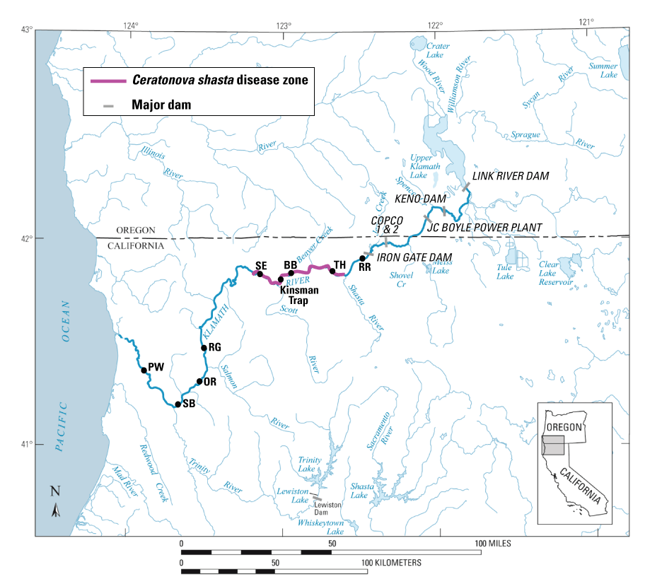
Locations of major tributaries, dams, the Kinsman fish trap upstream from the confluence with the Scott River, the Ceratonova shasta disease zone, and locations of two-dimensional hydrodynamic models used to model habitat of Chinook salmon (Oncorhynchus tshawytscha) on the Klamath River, Oregon and California. [Models: RR, R Ranch; TH, Trees of Heaven; BB, Brown Bear; SE, Seiad; RG, Rogers; OR, Orleans; SB, Saints Bar; PW, Pecwan.]
This report summarizes the simulated population dynamics of Klamath River juvenile Chinook salmon by running the S3 model under different disease and dam-removal scenarios. The primary goal of our analysis was to understand the near-term effects of dam removal in the first few years after dam removal. Although we noted many expected near-term effects on salmon production (for example, sedimentation of spawning gravels), consideration of all possible and long-term effects was beyond the scope of the analysis. The primary focus of NMFS was to understand how planned hatchery management and expected changes in C. shasta spore production under dam removal might influence production of salmon, which in turn, support endangered Southern Resident Killer Whales.
To support this focus, we constructed Dams In and Dams Out scenarios and structured model inputs specific to each scenario for nine index water years representing dry, average, and wet conditions. We also ran each dam-removal scenario under a low-spore and high-spore condition simulated by a spore production model that included factors such as flow pulses, water temperature, and prior-year prevalence of infection (POI) of hatchery fish (Robinson and others, 2022). We used spawner and juvenile abundances from an average salmon return year as inputs for all years, except for hatchery production under the Dams Out scenarios. Holding model inputs of salmon constant across scenarios allowed us to directly compare how simulated production of juvenile salmon varied among scenarios.
Study Site
The Klamath River Basin covers more than 15,000 square miles (mi2) and is divided into two subbasins (upper and lower) at Iron Gate Dam (river kilometer [rkm] 312; fig. 1). Although not a focus for this report, the upper basin area includes parts of Klamath, Lake, and Jackson Counties in Oregon, and Siskiyou and Modoc Counties in California. The lower basin area includes parts of the Siskiyou, Modoc, Trinity, Humboldt, and Del Norte Counties in California. The Klamath River Basin is unlike most watersheds, with a unique geomorphology opposite of that in most other drainage basins and has been called “a river upside down” by the National Geographic Society (Weddell, 2000; Rymer, 2008). Much of the upper Oregon section of the basin is flat and open, in comparison to the narrow canyons and mountainous terrain in the lower California section of the basin.
The upper Klamath River Basin lies in the rain shadow of the Cascade Range on the west, the Deschutes River Basin on the north, the Great Basin on the east, and the Pit River Basin on the south. The upper basin consists mostly of agriculture and rangeland with areas of pine forest and semiarid high-desert plateaus, and is characterized by low-relief, volcanic geology with an average annual precipitation of 88.6 centimeters (cm; California Rivers Assessment, 2011). The Klamath River is impounded by six dams, and four hydroelectric dams are being considered for removal (U.S. Department of Interior, 2013). Of the dams being considered for removal, the farthest upstream dam is Keno Dam (rkm 378.2) and the farthest downstream dam is Iron Gate Dam (rkm 312; fig. 1), which blocks the migration of anadromous salmon to the upper Klamath River Basin. The lower Klamath River Basin is mostly forested except for areas of agriculture and rangeland in the drainages of the Scott and Shasta Rivers. The lower Klamath River Basin is dominated by a steep, rugged, complex terrain (also known as the Klamath Mountains), and alluvial reaches. Average annual precipitation for the lower basin is 202.2 cm (California Rivers Assessment, 2011).
In this report, we focus on the section of the Klamath River between Keno Dam and the ocean. This section of the Klamath River is critical habitat used by several anadromous salmonids, including spring and fall run Chinook salmon, Coho salmon, and steelhead trout (Oncorhynchus mykiss). Additionally, several large tributaries contribute water and juvenile salmonids to the main-stem Klamath River. These tributaries are:
Methods
To run the dam-removal and disease scenarios, we used the version of the S3 model built specifically for Klamath River Chinook salmon populations. The key features of this model relevant to this report include (1) a C. shasta disease submodel; (2) habitat, river flow, and water temperature for Dams In and Dams Out scenarios; and (3) density-dependent dynamics that are influenced by the effect of flow on suitable habitat area. Perry and others (2019) noted that density-dependent movement fit observed abundance data better than a model with density-dependent survival. The disease submodel simulates (1) the probability of becoming infected with C. shasta and eventually dying from ceratomyxosis, and (2) the time to death of infected individuals. Infection and time to death are simulated as functions of time since initial exposure to C. shasta, water temperature, spore concentration, and duration of exposure (dose). With one exception, we ran the S3 model as described by Perry and others (2018) and parameterized by Perry and others (2019) and Plumb and others (2019). The singular difference in parameterization is that we reduced the maximum allowable exposure time from 14 to 7 days so as not to extrapolate exposure times beyond the observed data used to develop the disease model.
In this report, we briefly describe the model inputs and outputs as necessary to understand the structure of each scenario and the basic drivers of population dynamics under each scenario. We encourage readers to consult Perry and others (2019) for a complete description of the Klamath River S3 model; Perry and others (2018), which details the mathematical structure of the S3 model; and Plumb and others (2019), which focuses on the effect of flow management on disease-caused mortality.
Model Inputs
Habitat Template and Physical Inputs
The spatial domain of the S3 model is defined by a one-dimensional representation of discrete habitat units. In total, the Klamath S3 model comprises 378 river kilometers (rkm) and has 2,635 habitat units positioned between Keno Dam and the ocean, each of which were classified as specific mesohabitat types such as riffles, runs, pools, and braided channels (Perry and others, 2019). The 312-km section of river between Iron Gate Dam and the ocean consists of 1,706 discrete habitat units. For more detailed information on how meso-habitat units were determined for impounded and unimpounded sections of the Klamath River, readers are encouraged to consult Hardy and Shaw (2011).
The S3 model requires two physical inputs (water temperature and stream flow) that drive population dynamics either directly or indirectly. Daily water temperature dictates biological rates of development such as maturation of eggs in the gravel, growth of juveniles after emergence, and disease susceptibility and mortality owing to C. shasta. River discharge affects available habitat for juveniles, and, in turn, density-dependent dynamics (Perry and others, 2019). Additionally, river discharge affects habitat suitability of the annelid worm Manayunkia occidental, the intermediate host for C. shasta, which, in turn, affects the concentration of spores released by the annelid.
We used existing flow and temperature modeling datasets to construct model inputs for Dams In and Dams Out scenarios. For the Dams Out scenarios, we leveraged the effort of Perry and others (2011), who developed the River Basin Model 10 water temperature model and used it to simulate water temperatures for water years 1960–2009 under a Dams Out scenario condition using simulated daily flows provided by Reclamation as model input (Greimann and others, 2011). For the Dams In scenarios, we used simulated flows and water temperatures from Plumb and others (2019), which was produced for evaluating the Reclamation-proposed action for operating Klamath River hydroelectric projects. The Reclamation-proposed action includes water-management prescriptions that arose from a process of iterative application of the Klamath Basin Planning Model (KBPM). The KBPM simulates Klamath Project operations over a hydrologic period of record that includes water years 1981–2016.
To use the existing flow and temperature outputs from these previous efforts, we identified 9 years in common for each scenario representing dry (1992, 1994, and 2001), average (2007, 2008, and 2009), and wet (1996, 1998, and 2006) water years. These water years were selected in consultation with the NMFS and FWS. Simulated daily mean water temperatures at 20 locations for each scenario (Dams In, Dams Out) were used as input to S3 (fig. 2).
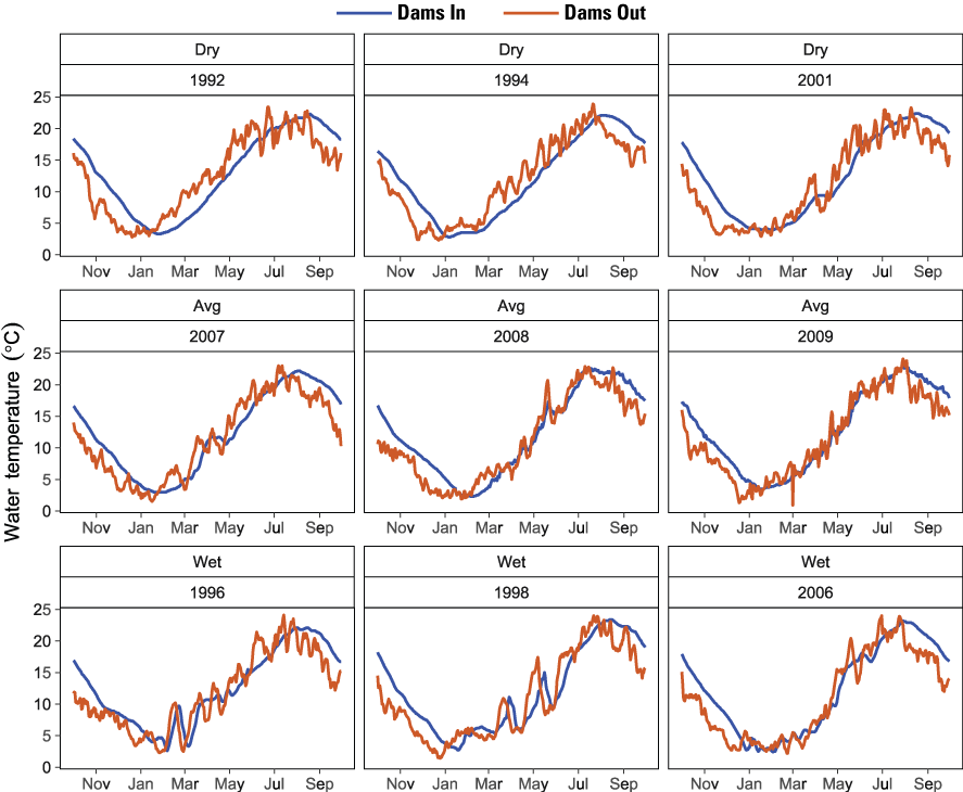
Daily mean water temperature at Iron Gate Dam simulated by River Basin Model 10 for Dams In (from Plumb and others, 2019) and Dams Out (from Perry and others, 2011) scenarios, Klamath River, California, water years 1992–2009. [°C, degrees Celsius]
For flow inputs to S3, we first compared and evaluated the suitability of simulated daily flows that were available for Dams Out (Greimann and others, 2011) and Dams In (Plumb and others, 2019; fig. 3) scenarios. After review, we had two concerns with using the flow produced by Greimann and others (2011) for the Dams Out scenarios. First, although monthly mean discharge was downscaled to daily mean discharge, monthly “steps” in the daily discharge were still evident in the simulated flow data (fig. 3), which did not match the true underlying pattern of variation in daily flow data. Second, the flows from Greimann and others (2011) did not include more recent water-management actions that implement annual flushing flows intended to scour annelid habitat and reduce C. shasta spore concentrations. Following discussion with our Federal agency working group, we decided to use the more recent Dams In flow simulations from Plumb and others (2019) for the Dams In and Dams Out scenarios, which included flushing flows as a management action. The rationale behind this decision is that managed flushing flows from Keno Dam would still be an important component of disease management after dam removal.
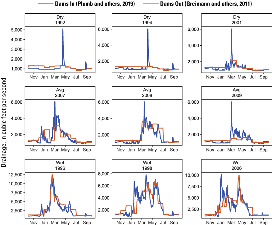
Simulated mean daily discharge at Iron Gate Dam used for the Dams In and Dams Out scenarios (Dams In from Plumb and others, 2019) compared to discharge produced by Greimann and others (2011) to represent a Dams Out condition, Klamath River, California, water years 1992–2009.
Here, we briefly describe how the flow simulations constructed by Reclamation, used in Plumb and others (2019), and used in this report were developed. Interested readers are encouraged to consult details in the Klamath Project Operations Final Biological Assessment (Bureau of Reclamation, 2019) and the NMFS Biological Opinion (National Marine Fisheries Service, 2019). First, for each annual simulation, hydrologic conditions and Upper Klamath Lake inflow forecasts were assessed, and then total water supply was allocated for Klamath Project delivery, storage in Upper Klamath Lake, or release to the Klamath River through an environmental water account (EWA). Next, for the period March 1–September 30, the EWA volume was distributed daily to the Klamath River with an overall goal of minimizing disease risk and providing habitats required for rearing and migration of salmonids (National Marine Fisheries Service, 2019). Under this proposed action, disease mitigation flows were intended to disrupt the complex life cycle of C. shasta by adversely affecting the abundance of annelid worms and their habitats through the release of surface flushing flows from Iron Gate Dam that met or exceeded 6,030 cubic feet per second (ft3/s) for at least 72 consecutive hours (Som and others, 2016). Distribution of the EWA targeted to address habitat needs was allocated through an approach aimed to mimic some characteristics of a natural flow regime (National Marine Fisheries Service, 2019). Flushing flows were accomplished by balancing remaining EWA volume with the number of days remaining in the management period and specified minimum flows that change each month, and then scaling river flows to observed inflows into Upper Klamath Lake (National Marine Fisheries Service, 2019).
The S3 model required flow inputs as a time series of daily mean discharge for discrete reaches of the simulated spatial extent in S3. For the Dams In scenarios, daily river flows were constructed from simulated Iron Gate Dam releases and historical gaged tributary inputs. Accretions from ungaged tributaries were estimated by apportioning unassigned gaged flows of the Klamath River in proportion to the watershed area of ungaged tributaries (Perry and others, 2019). For the Dams Out scenario that used the Dams In flows from Plumb and others (2019), we used the same approach for accretions downstream from Iron Gate Dam, but we also needed to simulate river flows for the unimpounded reach between Keno Dam and Iron Gate Dam. To estimate flows upstream from Iron Gate Dam, we used the flows from Greimann and others (2011) to calculate the relation between flows at Iron Gate Dam and upstream control points. We found that Klamath River flows upstream from Iron Gate Dam were strongly linearly related to flows at Iron Gate Dam (fig. 4), which allowed us to estimate upstream flows as a fraction of the flow at Iron Gate Dam.
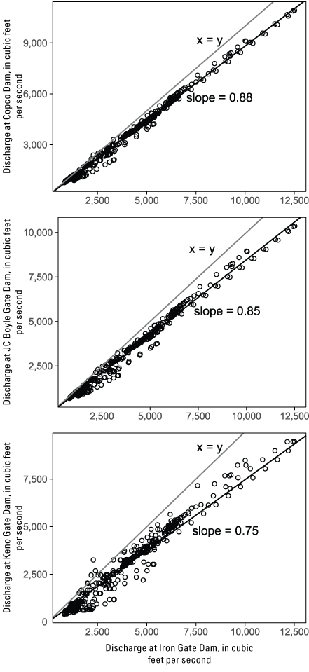
Relation between discharge at Iron Gate Dam and discharge at upstream locations under the Dams Out scenario simulated by Greimann and others (2011), Klamath River, California.
Inputs for the S3 model also require relations between discharge and the amount of suitable habitat for each habitat unit in the model domain. The available habitat area for each unit was quantified using an extrapolation procedure that scaled weighted usable habitat area curves constructed from two-dimensional hydrodynamic models for eight distinct geomorphic reaches of the Klamath River (see fig. 1) to each habitat unit of the S3 model domain (Perry and others, 2019). This extrapolation procedure was applied to the time series of river flows for each scenario to develop a time series of available habitat.
Biological Inputs
The S3 model relies on three primary forms of biological inputs to simulate population dynamics: (1) female spawners, (2) juvenile fish entering from tributaries and hatchery releases, and (3) a daily time series of spore concentrations. We used the same spawner and juvenile inputs for every water year, with some modifications between scenarios that account for the expected effect of dam removal on returns to Iron Gate Hatchery, hatchery releases, and the spatial distribution of spawning. We used spawner and juvenile inputs from brood year 2009 (juveniles outmigrating in water year 2010), which was the year that had the median escapement of natural spawners in the main-stem Klamath River from 2005 to 2018.
Female Spawners
We used the brood year 2009 estimate of 3,982 female spawners (Gough and Som, 2015) as inputs for Dams In and Dams Out scenarios, although for Dams Out scenarios, we allowed fish to spawn upstream from Iron Gate Dam. For the Dams In scenarios, spawner survey data were summarized as a weekly time-series of redd counts or female abundance estimates by survey reach (Gough and Som, 2015). To form model inputs for S3, weekly reach-level redd counts were distributed uniformly across days within each week and then assigned to each habitat unit in proportion to available spawning area within each survey reach (fig. 5; Perry and others, 2019). Surveys were not conducted downstream from rkm 178 owing to low use of the lower Klamath River for spawning. Therefore, we assumed that no spawning occurred downstream from rkm 178.
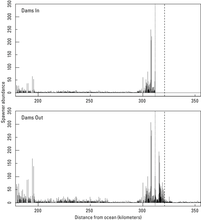
Spatial distribution of natural-origin female spawners in the main-stem Klamath River under Dams In (top graph) and Dams Out scenarios (bottom graph), Klamath River, California. [Dotted line marks the location of Iron Gate Dam, and the dashed line marks the location of Fall Creek.]
For the Dams Out scenario, which is intended to emulate conditions 1–3 years following dam removal, we shifted the spatial distribution of spawning by assuming that fish would move upstream from the dam but that spawning would be concentrated around the historical location of peak spawning densities near Iron Gate Dam. To achieve this distribution, we first assumed that one-half of the spawners in the 66-km reach below Iron Gate Dam would spawn in the 66-km free flowing reaches upstream from Iron Gate Dam. These spawners were then spatially distributed upstream from the dam in reverse proportion to their downstream spatial distribution (fig. 5). That is, we reversed the relative proportions of spawners in each habitat unit downstream from the dam and applied these proportions to the reach upstream from the dam to distribute spawners upstream from the dam. This approach had the desired effect of allowing spawning upstream from the dam but accounted for the idea that spawning would still be concentrated near the dam because all returning adults would have been progeny of spawners constrained to spawn downstream from Iron Gate Dam.
Because Iron Gate Hatchery will cease to operate once dams are removed, adults returning to Iron Gate Hatchery from juvenile releases within 3 years prior will be allowed to spawn in the wild (Klamath River Renewal Corporation, 2021). To simulate this aspect of dam removal, we allowed the 5,816 female spawners that returned to Iron Gate Hatchery in 2009 (Rushton, 2010) to naturally spawn in the main-stem river under the Dams Out scenarios. These additional natural spawners were distributed temporally and spatially identically to the spatiotemporal distribution of natural-origin spawners. We tracked naturally produced juveniles from hatchery spawners as a separate source population in S3 to understand how this component of natural production contributed to overall production.
Juveniles from Tributaries
In addition to the main-stem Klamath River and Iron Gate Hatchery, seven other source populations from major tributaries contributed juveniles to the Klamath River:
-
Bogus Creek,
-
Shasta River,
-
Scott River,
-
Salmon River,
-
Trinity River,
-
Trinity River Hatchery, and
-
Fall Creek Hatchery under Dams Out scenarios.
Except for the Salmon River, weekly abundance estimates and mean size of juveniles entering the Klamath River in water year 2010 were obtained from agencies that operated juvenile fish traps on tributary streams (fig. 6). The FWS provided abundance estimates for Bogus Creek and the Trinity River (Gough and others, 2015). California Department of Fish and Wildlife provided abundance estimates for the Shasta and Scott Rivers (for example, see Daniels and others, 2011). For constructing model inputs, all weekly abundance estimates were distributed uniformly across days within each week. For the Salmon River, we predicted weekly abundance estimates by applying a stock-recruitment model (see Plumb and others, 2019) to estimates of adult escapement provided by the Karuk Tribe. We used historical screw trap data for the Salmon River to estimate mean weekly size of juveniles entering the Klamath River from the Salmon River. Juvenile inputs from tributaries were held constant for all years and scenarios.
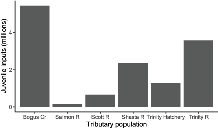
Estimated total abundance of juvenile Chinook salmon (Oncorhynchus tshawytscha) entering the Klamath River, California, from tributaries in water year 2010. [Cr, Creek; R, River]
Juveniles from Hatchery Production
Assuming the Federal Energy Regulatory Commission approves dam removal, Klamath River hatcheries will undergo a major shift in operations once dams are removed. Iron Gate Hatchery will be shut down when dams are removed and fish production activities will be relocated to Fall Creek Hatchery, about 11.2 km upstream from Iron Gate Dam. Fall Creek Hatchery will operate for 8 years following dam removal to facilitate fish recolonization of newly available habitat, although production of juvenile Chinook salmon will decrease from the target of 6 million juveniles at Iron Gate Dam to 3.25 million at Fall Creek Hatchery (Klamath River Renewal Corporation, 2021).
To simulate this shift in hatchery operations in S3, we used the Iron Gate Juvenile production in water year 2010 for Dams In scenarios and the planned production from Fall Creek Hatchery for Dams Out scenarios (table 1). Release numbers and mean size were obtained from Iron Gate Hatchery (Rushton, 2010) and distributed uniformly across days within the corresponding release week. In 2010, hatchery fish were released over a 3-week period with most fish being released on the first and third weeks of release in June (fig. 7).
Table 1.
Hatchery releases used as inputs to Stream Salmon Simulator (S3) for the Dams In and Dams Out scenarios, Trinity River. California, 2010.[For Iron Gate Hatchery, numbers in parentheses represent range of mean length for different release groups in 2010]
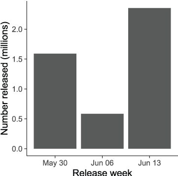
Weekly number of juvenile Chinook salmon (Oncorhynchus tshawytscha) released from Iron Gate Hatchery, Klamath River, California, in 2010.
For Dams Out scenarios, planned production goals of Fall Creek Hatchery were used to form model inputs (table 1; Klamath River Renewal Corporation, 2021). However, target release dates encompassed broad timeframes because actual releases from Fall Creek are to be timed with favorable river conditions (Klamath River Renewal Corporation, 2021). Therefore, we selected narrower release periods within these timeframes for our simulation (table 1).
Ceratonova shasta Spore Concentrations
To simulate infection and mortality of juvenile salmon caused by C. shasta, S3 requires inputs of daily C. shasta spore concentrations. Therefore, we developed a daily time series of spore concentrations using a three-part mechanistic model that captures key features of spore concentration dynamics such as week of initial spore detection, the seasonal pattern in spore density, and peak spore density (Robinson and others, 2022). The first part of the model (that is, first module) predicts onset of detectable spores using a degree-day model that begins accumulating degree-days at the median week of adult spawning in the fall prior to juvenile outmigration. The second module predicts the seasonality of spore concentrations using a quadratic function of water temperature. The third module predicts the annual peak spore concentration as a function of two variables, (1) the POI of hatchery-origin Chinook salmon juveniles in the previous year, and (2) the occurrence of flushing flows greater than or equal to 6,030 ft3/s for at least 72 consecutive hours.
To apply this model to our scenarios, we used historical spawning dates and the simulated flows and temperatures, yet we needed to set values for the prior-year POI of hatchery fish that bracketed the range in observed POI. Therefore, we constructed two spore scenarios, a “Low Spore” and “High Spore” scenario by setting the prior-year POI of hatchery fish to 0.15 and 0.75, respectively. These levels correspond to POI values observed in the year prior to water years with low spore concentrations (POI = 0.15) and years with very high spore concentrations (POI = 0.75). The median week of spawning was set to 45, which corresponded to November 2–8 in brood year 2009.
Running the spore model with these settings led to similar spore concentration patterns among all water years except 1992 and 1994. In 1992, simulated flushing flows were unable to achieve the minimum of 6,030 ft3/s for 72 consecutive hours because of water-availability constraints, which are a key trigger that reduces annual spore concentrations in the spore model. For 1992, spore concentrations exceeded 6 spores per liter (spores/L) for the Dams In and Dams Out Low Spore scenarios (fig. 8) and 400 spores/L for the Dams In and Dams Out High Spore scenarios (fig. 9). In 1994, there was an early peak in spores under the Dams Out Low Spore and High Spore scenarios that was not observed in other years. For this water year, the predicted week of spore release was week 12 (mid-March), but the flushing flow did not occur until week 14 (early April), which allowed spore concentrations to increase until the date at which the flushing flow occurred. All other years achieved the minimum flushing flow and thus had a similar pattern among years with little difference between scenarios. For these years, maximum spore concentrations were less than 1 spore/L for the Dams In and Dams Out Low Spore scenarios (fig. 8) and from 40 to 50 spores/L for the Dams In and Dams Out High Spore scenarios (fig. 9).
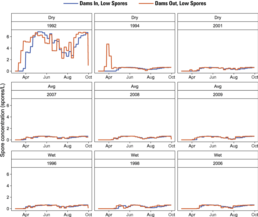
Simulated spore concentration for the Dams In and Dams Out Low Spore scenarios using the model of Robinson and others (2022) with the prior-year prevalence of infection of hatchery origin juvenile Chinook salmon (Oncorhynchus tshawytscha) set to 0.15, Klamath River, California, water years 1992–2009. [spores/L, spores per liter]

Simulated spore concentration for the Dams In and Dams Out High Spore scenarios using the model of Robinson and others (2022) with the prior-year prevalence of infection of hatchery origin juvenile Chinook salmon (Oncorhynchus tshawytscha) set to 0.75, Klamath River, California, water years 1992–2009. [spores/L, spores per liter]
Sensitivity Scenarios
In addition to our four primary scenarios, we ran two additional scenarios intended to understand the range of possible outcomes under certain model assumptions. First, to understand how complete elimination of disease would affect juvenile salmon abundance relative to the other two spore scenarios, we ran the Dams In and Dams Out scenario with C. shasta spore concentration set to zero. Second, for Iron Gate Hatchery releases, we investigated the sensitivity of the model to size-at-release of hatchery fish. In our primary scenarios, we used the historical release date, fish sizes, and release numbers that occurred in 2010. Although size-at-release in 2010 (table 1) was similar to the mean size across years (73 millimeters [mm]), we noted that the mean size in recent years was substantially smaller (approximately 67 mm). Therefore, to understand how size-at-release influenced abundance at the ocean, we ran two additional sets of scenarios using the minimum (66 mm) and maximum (79 mm) mean annual length in place of the length of fish released in 2010.
Stream Salmonid Simulator Output and Summaries
For each year, S3 simulates the daily abundance and mean size of fish in each life stage (fry, parr, and smolt) from each source population in each habitat unit. Because different populations are affected differentially by dam removal, we aggregated populations into three distinct population groups for summarizing model output: (1) tributaries, (2) main-stem natural spawners, and (3) Klamath River hatcheries. For the six tributary populations, model inputs (abundance, size, and timing of juveniles entering the main stem) are identical between all scenarios with the only difference being the water temperature and spore concentration of each scenario. In addition to these differences, main-stem natural spawners are allowed to spawn above Iron Gate Dam and spawners that would have returned to Iron Gate Hatchery are allowed to spawn naturally under Dams Out scenarios. Hatchery operations will change under Dams Out scenarios with a change in the hatchery location, total juvenile production, and release size and timing.
Because juvenile salmon abundance is tracked spatially and temporally, the daily abundance of fish passing any given location can be summarized over a day, week, migration season, or year. The primary location of focus for this analysis was the mouth of the Klamath River at the Pacific Ocean (rkm 0) because the status of juvenile salmon populations at ocean entry provides insight into food resources potentially available to Southern Resident Killer Whales.
To compare S3 model output between scenarios, we calculated total abundance and annual survival to the ocean using the simulated abundances of fish from each tributary source. Survival was calculated as the simulated annual fish abundance (N) in year y from source k passing location l under scenario f, divided by the initial annual abundance of fish that emerged as fry within the Klamath River or that entered the Klamath River from tributaries (NT):
This calculation allows for the comparison of annual survival for fish originating from different tributary and hatchery sources or summarized over multiple population sources for each scenario.
To quantify the prevalence of infection (POI) from S3 model output, we divided the simulated annual abundance of infected fish (I) in year y that originated from source k and passed location l under scenario f by the total annual abundance (N):
This calculation allows for the comparison of the fraction of infected fish that originated from different sources at a specific location of the Klamath River under each scenario.
The S3 model also tracks the daily number and location of infected fish that die because of C. shasta. We summarize this model output in two ways. First, we plotted the spatial distribution of mortality owing to C. shasta, as this information helps in understanding how quickly disease-caused mortality occurs and where infected fish ultimately succumb to C. shasta. Second, we calculated the proportion of the total mortality that was caused by C. shasta. This metric helps to determine the amount of mortality caused by C. shasta relative to other causes such as natural mortality or thermally induced mortality.
Understanding how the S3 disease model works is important for interpreting in-river mortality, the prevalence of infection at ocean entry, and the differences among the scenarios. The S3 disease model is based on analysis of extended sentinel trials where exposure times of juvenile salmon to C. shasta were varied from 1 to 7 days (Perry and others, 2019). The S3 disease model consists of two parts: (1) the probability of becoming infected and dying because of C. shasta, and (2) the time from initial exposure to death. The first part of the model predicts the proportion of fish that will eventually die from C. shasta, which is estimated from the total mortality observed in each sentinel trial. In S3, the first part of the model transitions fish from non-infected to infected fish that will eventually die but are not yet dead. In the second part, infected fish die based on the time lag between infection and eventual death (Perry and others, 2019).
When evaluating scenarios, both the difference in survival and prevalence of infection should be considered because infected fish are those that would be expected to eventually die based on our modeling of the extended sentinel experiments. For example, the prevalence of infection at ocean entry indicates fish that would be expected to eventually die, but their time to death was such that they arrived at the ocean before death occurred. Migration rates in S3 are driven, in turn, by (1) fish size (which is affected by water temperature and fish growth rates), and (2) habitat availability and fish density. Therefore, whether infected fish die in-river depends on the interplay between their predicted time-to-death and population-specific migration rates as driven by growth rates and fish size.
Results
Because production of juvenile salmon available to Southern Resident Killer Whales is the primary interest of this work, we begin by first presenting model output of annual abundance of juvenile salmon entering the Pacific Ocean. We then follow with inter-annual and intra-annual summaries of population dynamics that help to understand factors driving annual variation in production and differences among scenarios.
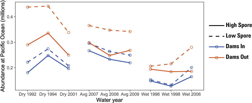
The S3 model simulated considerably higher total abundance for Dams Out scenarios relative to the respective Dams In scenarios and higher abundance for Low Spore scenarios relative to High Spore scenarios (fig. 10). The difference in total abundance between scenarios was highest in dry water years and lowest in wet water years. In contrast, there was less difference among water years between spore scenarios, with the largest difference being nearly 1 million fewer fish for the Dams Out with High Spore scenario in 1992, the only year in which flushing flows did not meet the 6,030 ft3/s criteria required for scouring annelid habitat and reducing C. shasta spore concentrations. Abundance for the No Spore scenarios was nearly identical to abundance for the Low Spore scenarios, indicating little disease-caused mortality under the Low Spore scenarios (fig. 10).
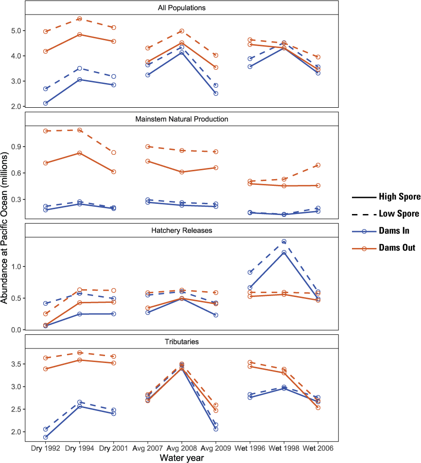
Simulated abundance of juvenile Chinook salmon (Oncorhynchus tshawytscha) at the Pacific Ocean for Dams In and Dams Out scenarios, Klamath River, California, water years 1992–2009.
The difference in abundance between dam-removal and spore scenarios varied among population groups. For main-stem natural production, abundance of juveniles at ocean entry was 2–3 times higher under Dams Out scenarios (fig. 10). Although additional spawners from fish that would have returned to Iron Gate Hatchery contributed substantially to this difference under Dams Out, juvenile production from naturally produced spawners was also higher under Dams Out (app. 1, fig. 1.1). For main-stem natural production, abundance for the High Spore scenario was considerably lower than the Dams Out Low Spore scenario, but there was little difference between spore scenarios for Dams In. For Hatchery releases, abundance at ocean entry was similar between Dams In and Dams Out scenarios for most water years, despite smaller release sizes from Fall Creek Hatchery under Dams Out (fig. 10). For tributary populations, abundance for the High Spore scenarios was consistently lower than Low Spore scenario, but differences between dam-removal scenarios varied considerably among water years, with Dams Out scenario having similar or higher abundance than the Dams In scenario, and dry water years having the largest difference between the Dams In and Dams Out scenarios.
For all populations combined, survival to the ocean ranged from about 8 to 15 percent but varied considerably among population groups and scenarios (fig. 11). As expected, survival for Low Spore scenarios was higher than High Spore scenario for all population groups. Among population groups, juveniles originating from main-stem natural production had the lowest survival from the time to emergence to ocean entry, ranging from about 1 to 5 percent, whereas hatchery releases had survival rates ranging from near zero to 30 percent. This difference among population groups is driven by the life stage at which juveniles enter the model; that is, as fry for the main-stem, but as larger smolts for the hatchery. For main-stem natural production, survival for the Dams Out scenario was higher than the Dams In scenario, explaining the difference in abundance between scenarios. For hatchery releases, survival for the Dams Out scenarios were higher than the Dams In scenarios for all years except 1998. Given the lower hatchery production under the Dams Out scenarios, higher survival helps explain why abundance at ocean entry was similar between Dams In and Dams Out scenarios.
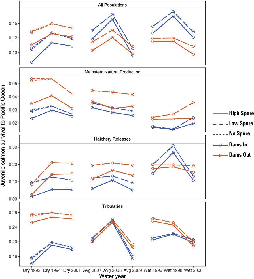
Total survival of juvenile Chinook salmon (Oncorhynchus tshawytscha) to the Pacific Ocean for Dams In and Dams Out scenarios, Klamath River, California, water years 1992–2009.
In addition to total abundance, the S3 model tracks the number of infected fish that die within the main-stem Klamath River and infected fish that survive to the ocean. These metrics provide important context about levels of in-river mortality caused by disease, and the health and potential fate of fish entering the ocean, because infected fish are expected to eventually die from ceratomyxosis. First, almost none of the in-river mortality was caused by C. shasta for the Low Spore scenario (fig. 12). Second, among populations for High Spore scenarios, a higher proportion of the total mortality of hatchery releases was caused by C. shasta relative to main-stem natural production. For hatchery releases, in-river mortality owing to C. shasta was higher under the Dams In relative to the Dams Out scenarios, further highlighting why hatchery fish had higher survival rates under the Dams Out scenarios, resulting in similar abundance at ocean entry. In contrast, for main-stem natural production, although total mortality for the Dams Out scenarios were lower than for the Dams In scenario (fig. 11), a higher proportion of the in-river mortality was caused by C. shasta for the Dams Out scenario (fig. 12).
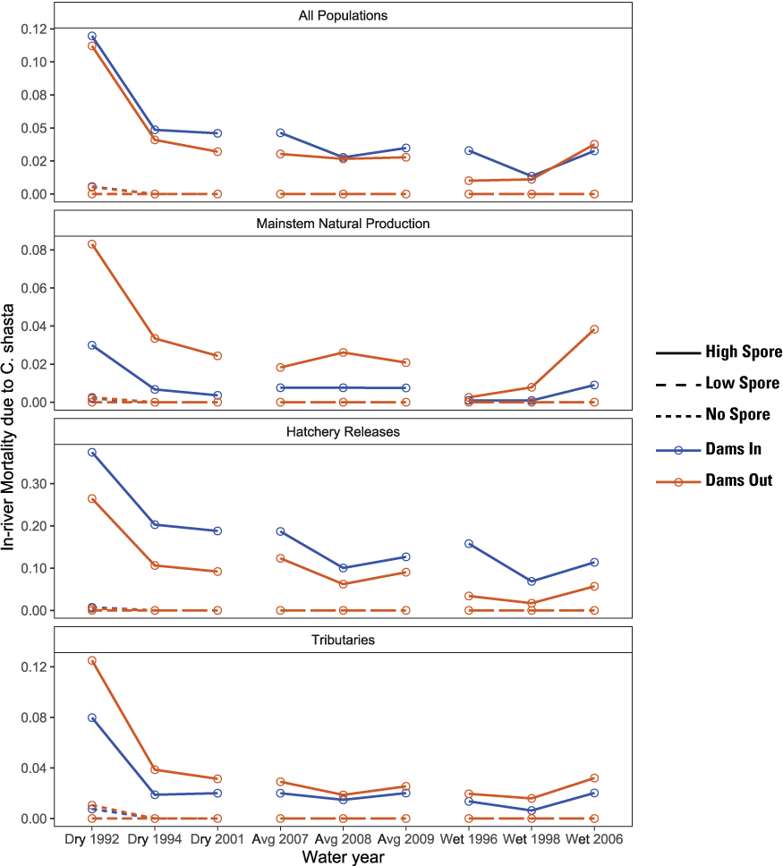
Proportion of the total in-river mortality of juvenile Chinook salmon (Oncorhynchus tshawytscha) caused by Ceratonova shasta, by water year, for Dams In and Dams Out scenarios exposed to low and high prevalence of infection, Klamath River, California, water years 1992–2009.
The prevalence of infected fish at ocean entry varied overall from 0 to 6 percent for main-stem and tributary populations but was considerably higher for hatchery populations, varying from 0 to 60 percent (fig. 13). Specifically, under High Spore scenarios, the prevalence of infected hatchery fish at ocean entry varied from 20 to 60 percent in all years except 1992. Spore concentrations in 1992 were highest of all water years simulated; thus, the prevalence of infection in 1992 was zero because infected fish died in-river before arriving at ocean entry. Although hatchery fish contribute to total production of juvenile salmon entering the ocean, a much higher proportion of those fish could ultimately die after ocean entry relative to other population groups.
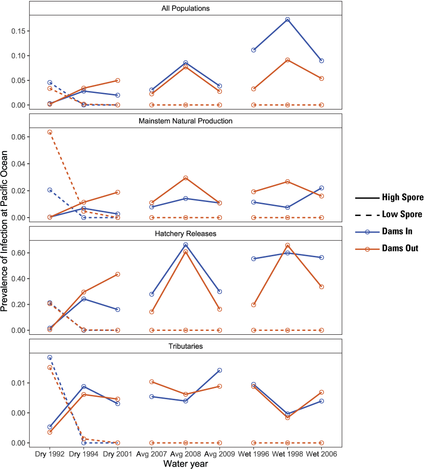
Simulated prevalence of Ceratonova shasta infection in juvenile Chinook salmon (Oncorhynchus tshawytscha) at the Pacific Ocean for Dams In and Dams Out scenarios, Klamath River, California, water years 1992–2009.
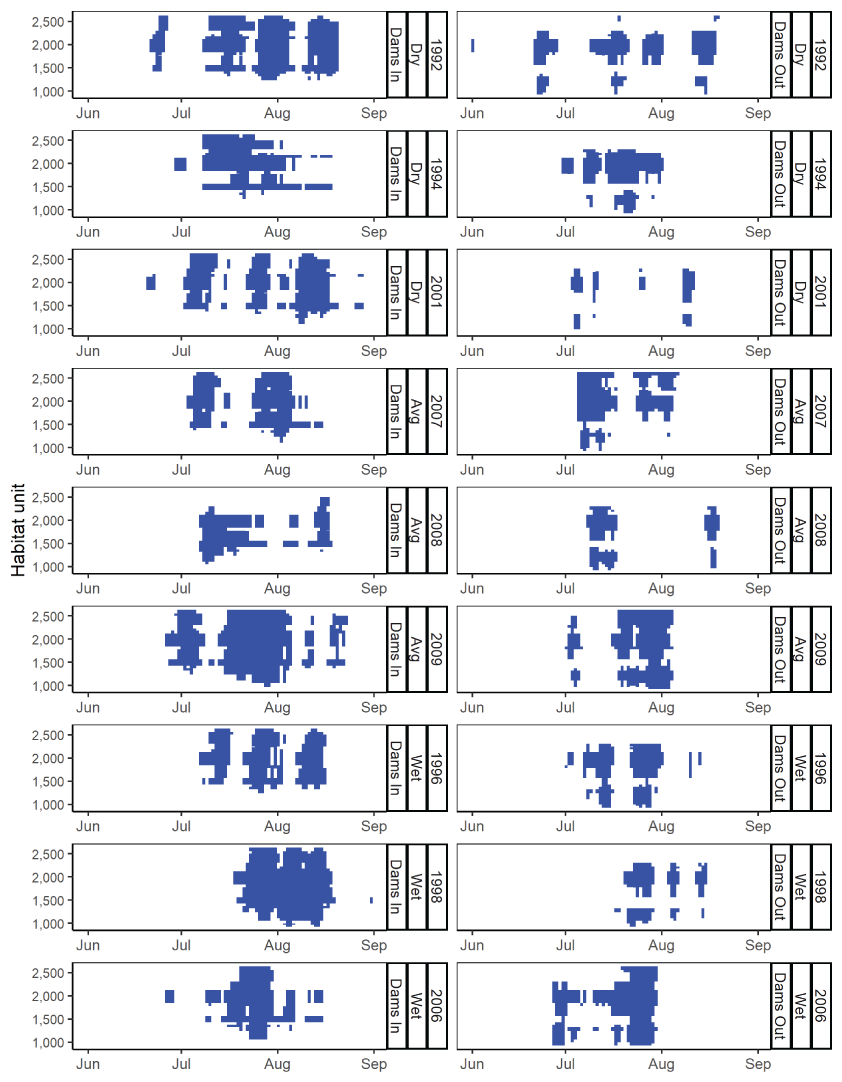
The S3 model also tracks where infected fish die within the main-stem (fig. 14). The location of mortality owing to C. shasta varied among years and scenarios, but for most water years, most disease mortality occurred downstream from the infectious zone. The exception was 1992, the year with the highest spore concentrations, where nearly all disease-caused mortality occurred within the infectious zone. Within years, the spatial distribution of disease-caused mortality was either similar between Dams In and Dams Out scenarios (for example, 1994, 2008, and 1996) or more of the mortality was within the infectious zone for Dams In scenarios (for example, 2001 and 2007).
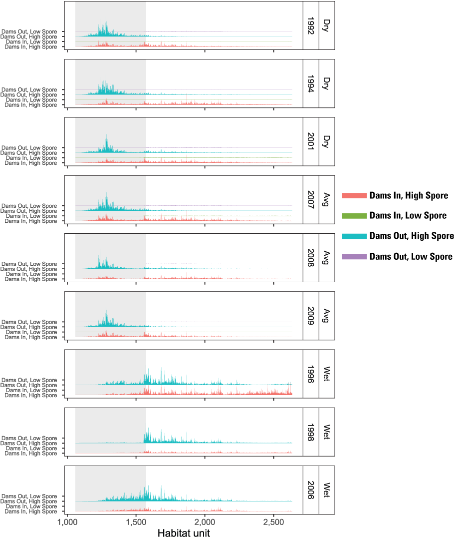
Spatial distribution of simulated mortality of juvenile Chinook salmon (Oncorhynchus tshawytscha) owing to Ceratonova shasta for Dams In and Dams Out scenarios, Klamath River, California, water years 1992–2009.
Egg survival, emergence timing, run timing, and size at ocean entry provide further insights into factors driving differences among years and scenarios. For main-stem natural production, egg survival varied by 10 percentage points from about 62 to 72 percent (fig. 15). For Dams In, survival tended to increase from dry to wet water years, likely owing to increased habitat area that reduced redd superimposition. In contrast, egg survival for Dams Out scenarios averaged about 65 percent and was slightly lower than Dams In scenarios for average and wet water years. Egg survival for the Dams Out scenarios were likely influenced by three factors: (1) a change in the thermal regime that increased incubation times, (2) more than a doubling of natural spawners owing to Iron Gate Hatchery returns, and (3) an upstream shift in spatial distribution of spawning.
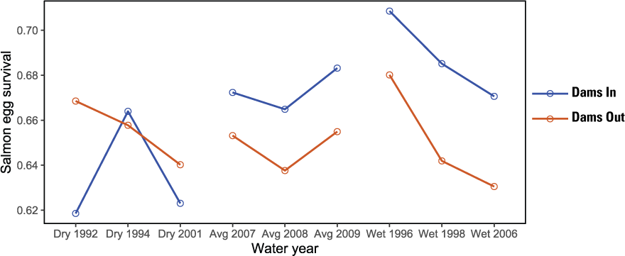
Proportion of Chinook salmon (Oncorhynchus tshawytscha) eggs surviving from spawning to emergence as fry for Dams In and Dams Out scenarios, Klamath River, California, water years 1992–2009.
The higher survival from emergence to ocean entry for main-stem natural production is what led to the higher abundance under the Dams Out scenarios – a result of three interacting factors: (1) emergence timing, (2) size at age, and (3) ocean entry timing. In short, under Dams Out scenarios, emergence timing tended to be later (fig. 16), yet fish size-at-date was similar or larger at ocean entry (fig. 17); and run timing was similar or earlier at ocean entry (fig. 18). These findings indicate that fish spent less time rearing, and therefore incurred less mortality, because they grew faster, attained larger size at age, and reached the ocean earlier owing to size- and density-dependent migration rates incorporated into S3.
Simulated emergence timing of juvenile Chinook salmon (Oncorhynchus tshawytscha) for Dams In and Dams Out scenarios, Klamath River, California, water years 1992–2009.
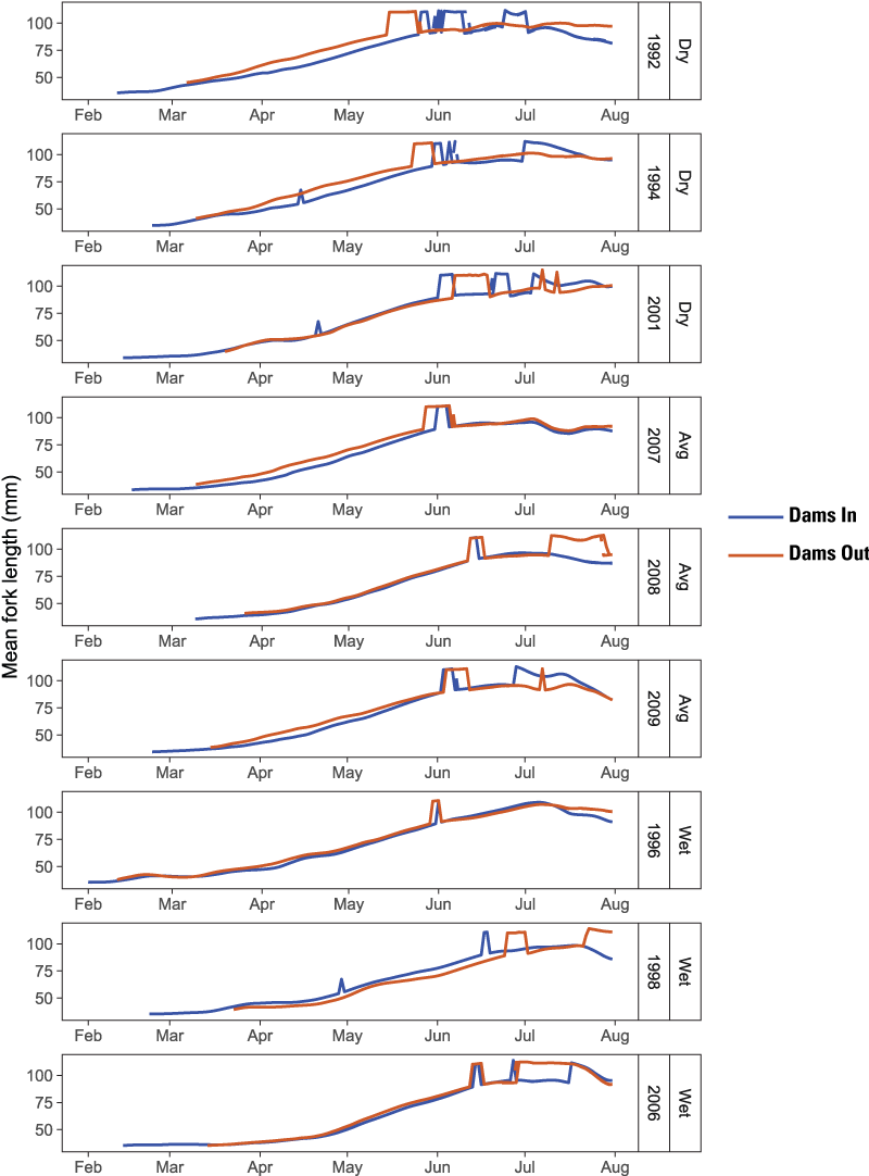
Simulated size of juvenile Chinook salmon (Oncorhynchus tshawytscha) at ocean entry for Dams In and Dams Out scenarios, Klamath River, California, water years 1992–2009.
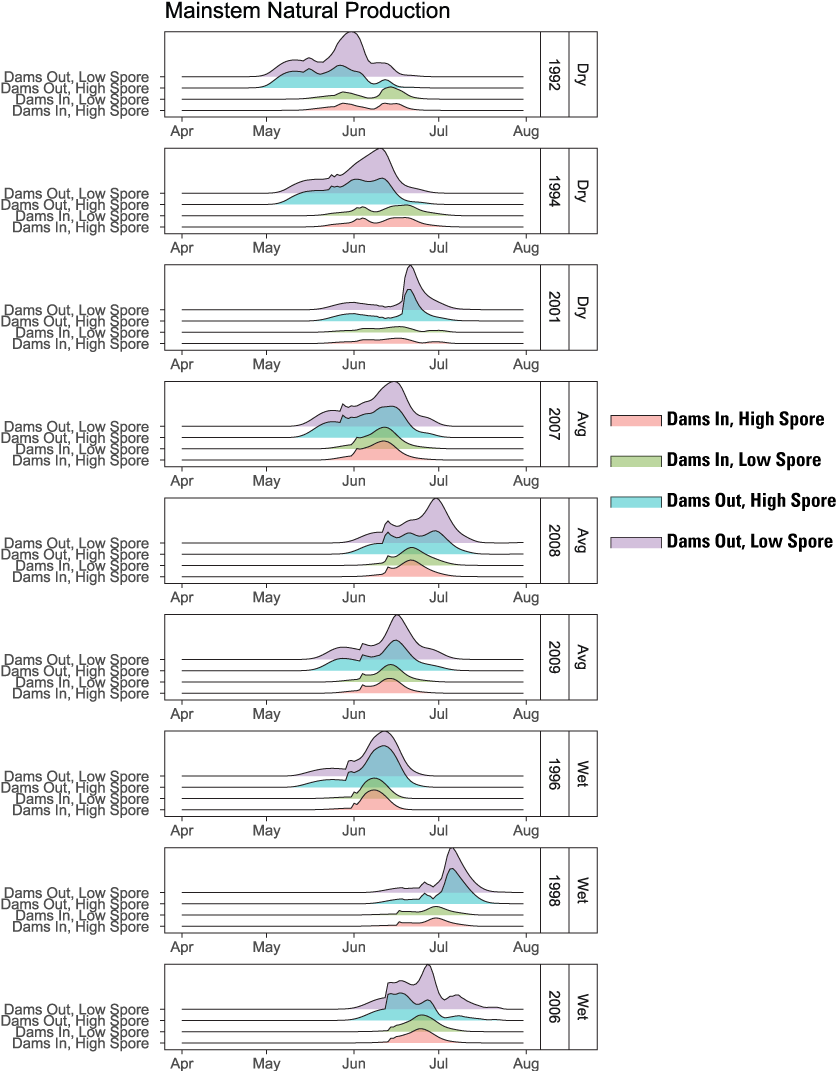
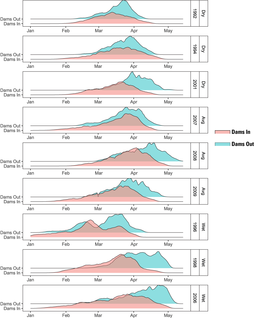
Run timing at ocean entry for juvenile Chinook salmon (Oncorhynchus tshawytscha) produced by spawning in the main-stem Klamath River for Dams In and Dams Out scenarios, Klamath River, California, water years 1992–2009.
Run timing of hatchery fish provides insights about differences in production among years and scenarios (fig. 19). First, under the Dams Out scenarios, an early (mid-May–mid-June) and late (late-June–July) pulse of fish at ocean entry was evident (fig. 19) owing to the Fall Creek Hatchery strategy of releasing fry in March and parr in June (table 1). Although the early group was a small proportion of outmigrants relative to the late group, this release strategy seems to have some benefit of spreading the mortality risk in high-disease years. For example, in 1992, the year with the highest spore concentrations, the early pulse of juveniles is on the same order of magnitude as the late pulse for both Low and High Spore Scenarios. For the Dams In scenarios, fish were released from Iron Gate Hatchery in two pulses (fig. 7), yet most years had a single pulse in ocean entry in late-June/early-July. However, 3 years (1992, 1996, and 1998) had a second later pulse in mid-July that represented a significant fraction of the outmigration. These were the only water years in which abundance of hatchery fish for Dams In scenarios were similar to or higher than the Dams Out scenarios (fig. 10). These findings suggest that the latest release group during the week of June 13–19 survived poorly in most water years. Furthermore, for years without this second pulse for both High and Low Spore scenarios, disease-caused mortality was not the probable cause of death for this group. This group instead likely experienced water temperatures greater than 24 degrees Celsius (°C), the point at which survival declines rapidly because of exceedance of thermal tolerance (fig. 20; Perry and others, 2018).
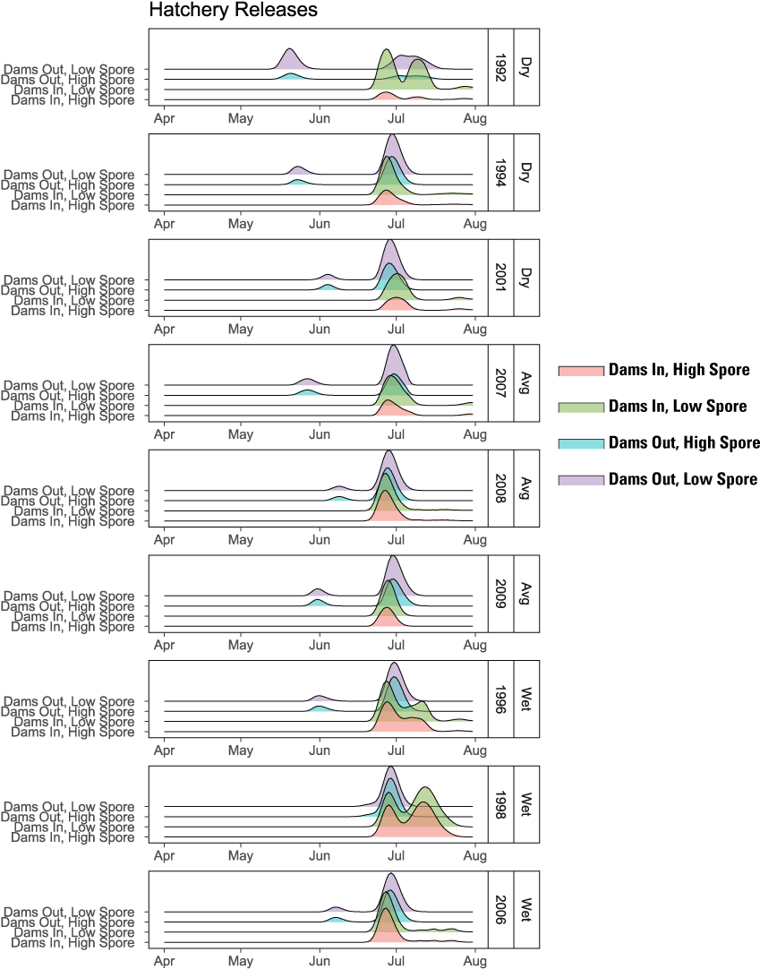
Run timing at ocean entry for hatchery releases of juvenile Chinook salmon (Oncorhynchus tshawytscha) for Dams In and Dams Out scenarios, Klamath River, California, water years 1992–2009.
Shaded regions showing locations and dates when simulated daily mean water temperatures exceeded 24 degrees Celsius for Dams In and Dams Out scenarios, Klamath River, California, water years 1992–2009.
Our sensitivity analysis indicated that the size at release of Iron Gate Hatchery fish had a large influence on their simulated abundance at ocean entry (fig. 21). Although abundance of hatchery fish was similar between Dams In and Dams Out scenarios, larger size at release from Iron Gate Hatchery under Dams In scenarios led to higher abundance at ocean entry compared to releases from Fall Creek Hatchery under the Dams Out scenarios. In contrast, smaller-than-average size at release from Iron Gate Hatchery led to lower abundance. This outcome was driven by two processes. First, because migration rate is size-dependent and survival is time-dependent in S3, larger fish migrate faster and therefore incur less in-river mortality. Second, because larger fish migrated faster than smaller fish in our simulation, the latest release group avoids the high water temperatures that caused high mortality in most water years for the brood year 2009 release group from Iron Gate Hatchery. For example, for the maximum mean annual size at release (79 mm), fish arrived at the ocean earliest and two distinct pulses occurred in most years, indicating that the latest release group did not incur the high mortality observed for brood year 2009 releases (fig. 22). In contrast, the minimum mean annual size at release (66 mm) arrived latest and survived poorly in all but wet water years, likely because all release groups encountered high water temperatures during their migration to the ocean.
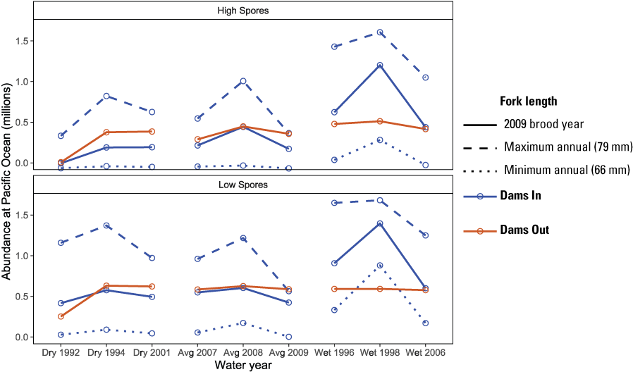
Effect of size at release on simulated abundance at the Pacific Ocean for hatchery origin juvenile Chinook salmon (Oncorhynchus tshawytscha), Klamath River, California, water years 1992–2009. [mm, millimeters]
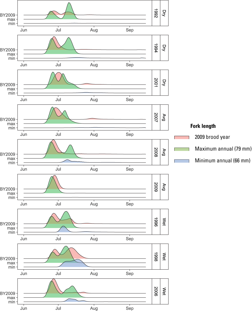
Effect of size at release on run timing at ocean entry for hatchery releases of juvenile Chinook salmon (Oncorhynchus tshawytscha) for the Dams In and Low Spores scenario, Klamath River, California, water years 1992–2009. [BY, brood year; max, maximum; min, minimum; mm, millimeters]
Discussion
The key findings from our simulations were that (1) total abundance of juvenile Chinook salmon at ocean entry for the Dams Out scenarios were higher than the Dams In scenarios under each respective spore scenario, (2) the difference in total abundance between dam-removal scenarios was highest in dry water years and lowest in wet water years, (3) abundance at ocean entry for the Low Spore scenario was higher than for the High Spore scenario regardless of the dam scenarios, and (4) the effect of each dam or spore scenario varied among population groups. Although we found that simulated abundance was higher under the Dams Out scenario, it is critical to cast this outcome in the context of (1) key assumptions underlying our analysis, (2) likely effects of near-term dam removal that were not included in our simulation, and (3) the effect of disease caused by C. shasta on mortality of fish entering the ocean.
The difference in total abundance between scenarios arises from the interplay of nine different population groups that each have a somewhat unique response to the scenarios owing to whether they are (1) of natural or hatchery origin, (2) main-stem or tributary spawners, (3) present in upper- or lower-river tributaries, and (4) exposed or not to the C. shasta infectious zone. For example, tributary populations had more similar abundances between scenarios for average water years than the other two population groups. Some of this difference is owing to tributary populations themselves being a mixture of six different populations with differential exposure to C. shasta. For example, in S3, only juveniles from Bogus Creek and the Shasta River travel through the entire infectious zone, juveniles from the Scott River travel through the lower end of the infectious zone, and all other tributaries enter the Klamath River downstream from the infectious zone. Thus, tributary populations that pass through the infectious zone contribute disproportionately to differences in abundance among the High and Low Spore scenarios.
Other causes of different abundance patterns contributing to total abundance are owing to differential effects of dam removal among populations. For example, under the Dams Out scenarios, the spatial distribution of main-stem spawners shifts upstream, additional spawners destined for Iron Gate Hatchery spawn naturally in the main stem, and incubating eggs develop under a shifted thermal regime after dam removal. These factors acted in concert to affect egg survival, the timing and location of emerging fry, their rate of growth and timing of movement downstream, and the timing and duration of their exposure to C. shasta. In contrast, tributary populations had identical size, abundance, and timing at which they enter Klamath River under all scenarios.
Klamath River hatchery populations have yet a different pattern of abundance owing to the shift in location and production strategy after dam removal. The most surprising outcome here was the similar abundance between Dams In and Dams Out scenarios in most water years despite changes in hatchery operation that would be expected to reduce abundance of hatchery origin fish post-dam removal (less fish produced, smaller size, released farther upstream). We found that comparable abundance between scenarios was caused by low survival owing to high water temperature experienced for the latest group released from Iron Gate Hatchery. Our sensitivity analysis on size at release further indicated how release timing and size-dependent migration rates interact to influence survival and exposure to high water temperatures that occur during most summers in the Klamath River.
Although our simulations identified similar abundance of hatchery fish at ocean entry between Dams In and Dams Out scenarios, our analysis indicated that this outcome was highly dependent on the mean size and release timing of fish that occurred in water year 2010. Historically, mean size at release varied considerably among years (fig. 23). Additionally, annual release timing from Iron Gate Hatchery has varied from mid-May to mid-June since 2005. Simulated spore concentrations tended to peak between mid-May and mid-June (fig. 9), but water temperatures continued to increase through July (fig. 2) and exceeded 24 °C across much of the river beginning in late-June to mid-July (fig. 20). Thus, release timing and size strongly influence C. shasta exposure duration and water temperatures encountered by juvenile salmon during downstream migration. Earlier releases at larger average sizes would tend to increase survival rates, resulting in more Iron Gate Hatchery fish surviving to the ocean relative to Fall Creek Hatchery fish owing to many more fish being released from Iron Gate Hatchery. However, our analysis indicates how late release timing and smaller sizes can lead to lower survival rates, negating the potential benefit of larger release sizes. Thus, the relative performance of hatchery programs pre- and post-dam removal should be considered in the context of release timing and size at release.
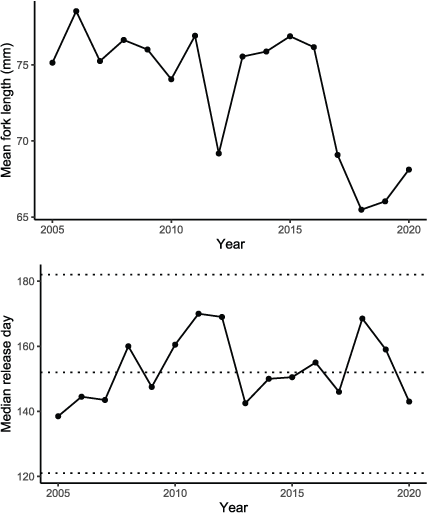
Mean annual fork length and median release day of hatchery juvenile Chinook salmon (Oncorhynchus tshawytscha) released from Iron Gate Hatchery, Klamath River, California, 2005–20. Dashed lines reference May 1, June 1, and July 1.
Our simulation clearly shows the benefit of flushing flows in years that would otherwise be predicted to have high spore concentrations owing to the prior year’s prevalence of infection of hatchery fish (Robinson and others, 2020). In all but one year, managed flushing flows met minimum criteria that triggered a reduction in spore concentration owing to scouring of annelid habitat. Therefore, even under the High Spore scenario, spore concentrations were moderate in most years (<50 spores/L) relative to 1992 when minimum flushing flows were not met (>400 spores/L). Effects of the moderate versus the very high spore concentrations of 1992 contrast sharply and differ among population groups. For all populations, the highest mortality owing to C. shasta occurred in 1992 relative to other years for the High Spore scenario (fig. 12). For main-stem natural production, the largest difference in abundance between spore scenarios occurred in 1992 (fig. 10). Owing to their late migration timing, hatchery origin fish had very low survival rates and abundance in 1992 relative to other populations that migrate earlier.
Differences in disease severity among years and populations in the High Spore scenario were evident in the prevalence of infected fish entering the ocean. In 1992, when spore concentrations exceeded 400 spores/L, the prevalence of infected fish entering the ocean was effectively zero, indicating that all infected fish died before entering the ocean. Most of this mortality occurred within the current infectious zone, whereas C. shasta-caused mortalities were distributed farther downstream in other years. The location of mortality is critical because fish that die may release myxospores that infect annelid worms, which subsequently release actinospores that infect salmon, perpetuating the disease cycle (Bartholomew and others, 1997).
In other years, when spore concentrations were moderate, the prevalence of infected fish entering the ocean remained low for juveniles from main-stem natural production (<3 percent) but was considerably higher for hatchery fish under Dams In and Dams Out scenarios (15–60 percent; fig. 13). This striking difference among populations was driven by many factors. Foremost, although moderate spore concentrations reduced infection rates relative to the high levels in 1992, lower spore concentrations also increase the time from infection to death (Ray and others, 2014; Perry and others, 2019). Thus, late migration of hatchery fish during warm water temperatures and peak spore concentrations led to high infection rates. However, the moderate spore concentrations increased time to death (relative to 1992 levels) and the larger size of hatchery juveniles (relative to naturally produced fish) led to faster migration rates, causing a high proportion of infected fish to arrive at the ocean prior to death. This finding is particularly important because infected fish are expected to die at some future point based on our analysis of sentinel exposure experiments (Ray and others, 2014; Perry and others, 2019). Thus, although the prognosis of infected fish entering the ocean is unknown, a high proportion of these fish possibly die before becoming available to Southern Resident Killer Whales as a food resource.
Our analysis was tailored to understand how the effects of two key factors (hatchery operations and disease) are likely to affect abundance of salmon available to Southern Resident Killer Whales following dam removal, but our analysis ignored numerous other expected effects of dam removal. Our analysis proceeded as if the only effects of dam removal were on (1) water temperatures; (2) spawner abundance, location, egg survival, and emergence timing; and (3) hatchery operations. However, many other effects ranging from immediate, to short term, to long term processes are likely to influence salmon population dynamics. For example, fine sediment may hamper spawning success, reducing egg survival and lowering the abundance of juvenile salmon relative to our simulations, which held egg survival rates constant between scenarios (Klamath River Renewal Corporation, 2021). Additionally, sedimentation of gravels and high turbidity may influence macroinvertebrate production, and turbidity may reduce feeding efficiency; both of which could influence growth rates of juvenile salmon. In contrast, consumption rates in our growth model were held constant in all scenarios in our analysis. Although we did not assess all likely effects of dam removal, by focusing on key changes of interest after dam removal (for example, disease, hatchery operations), we were able to compare effects of these changes while holding other factors (for example, turbidity) constant between scenarios.
In summary, our analysis found that total abundance of juvenile Chinook salmon at ocean entry was highest for all water years under the Dams Out and Low Spore scenarios. Although we conducted both low- and high-spore scenarios under Dams Out, we might expect spore concentrations to remain low in the first few years following dam removal because of scouring and smothering of annelid habitat. Thus, Low Spore scenario may be a more likely representation of future conditions following dam removal compared to the High Spore scenario. In contrast, the High Spore scenario under the Dams In scenarios simulated conditions that have been measured in the recent past and included a “worst-case scenario” simulated in 1992 when no flushing flows led to very high spore concentrations. Our analysis also indicated that the overall pattern of abundance at ocean entry was driven by population groups that had different responses to each scenario. Our analysis included nine distinct population groups, including main-stem spawners that will be directly affected by dam removal, hatchery populations that will undergo a major change in hatchery management, and tributary populations that are differentially affected owing to their spatial location in the watershed. The S3 model was able to track each of these populations and provide insights on how the differential responses of each population combined to influence the simulated number of juvenile Chinook salmon arriving at the Pacific Ocean where they become available as a food source for Southern Resident Killer Whale.
References Cited
Bartholomew, J.L., Whipple, M.J., Stevens, D.G., and Fryer, J.L., 1997, The life cycle of Ceratomyxa shasta, a myxosporean parasite of salmonids, requires a freshwater polychaete as an alternate host: The Journal of Parasitology, v. 83, no. 5, p. 859–868. [Also available at https://doi.org/10.2307/3284281.]
Bureau of Reclamation, 2019, Addendum to the proposed action included in Reclamation's 2018 final biological assessment on the effects of the proposed action to operate the Klamath Project on federally-listed threatened and endangered species: Document emailed to the National Marine Fisheries Service by the Bureau of Reclamation on January 24, 2022, [variously paged]. [Also available at https://www.usbr.gov/mp/kbao/docs/final-2018-ba-klamath-project-ops.pdf.]
California Rivers Assessment, 2011, Watershed information by basin, average precipitation per year: California Rivers Assessment, Watershed database, accessed January 24, 2021, at https://www.ice.ucdavis.edu/project/cara.html
Gough, S.A., David, A.T., and Pinnix, W.D., 2015, Summary of abundance and biological data collected during juvenile salmonid monitoring in the mainstem Klamath River below Iron Gate Dam, California, 2000–2013: U.S. Fish and Wildlife Service, Arcata Fish and Wildlife Office, Arcata, California, Arcata Fisheries Data Series Report Number DS 2015–43, 95 p. plus appendixes.
Greimann, B.P., Varyu, D., Godaire, J., Russell, Kendra, L., Talbot, R., and King, D., eds., 2011, Hydrology, hydraulics and sediment transport studies for the secretary’s determination on Klamath River Dam removal and basin restoration: U.S. Bureau of Reclamation, Mid-Pacific Region, Technical Service Center, Denver, Colorado, Technical Report No. SRH-2011–02, 762 p.
Hardy, T.B., and Shaw, T., 2011, SALMOD—Meso-habitat development Keno to estuary, in Hendrix, N., Campbell, S., Hampton, M., Hardy, T., Huntington, C., Lindley, S., Perry, R., Shaw, T., and Williamson, S., Fall Chinook salmon life cycle production model report to expert panel: Prepared for Expert Panel reviewing Chinook salmon of the Klamath River Basin, p. 4–1 to 4–32, accessed January 24, 2022, at https://www.fws.gov/arcata/fisheries/reports/technical/Fall%20Chinook%20Report%20of%2FPM%20Team%20to%20Expert%20Panel%20DRAFT%201%202011.pdf.
Klamath River Renewal Corporation, 2021, Lower Klamath Project biological assessment: Klamath River Renewal Corporation, accessed January 24, 2022, at http://www.klamathrenewal.org/wp-content/uploads/2021/03/A-1-Draft-BA.pdf.
National Marine Fisheries Service, 2019, Endangered Species Act Section 7(a)(2) biological opinion, and Magnuson-Stevens Fishery Conservation and Management Act essential fish habitat response for Klamath Project Operations from April 1, 2019 through March 31, 2024: Letter to Jeffrey Nettleton, Area Manager, Klamath Basin Area Office Bureau of Reclamation, accessed January 24, 2022, at https://www.fisheries.noaa.gov/resource/document/2019-klamath-project-biological-opinion.
Perry, R.W., Plumb, J.M., Jones, E.C., Som, N.A., Hardy, T.B., and Hetrick, N.J., 2019, Application of the Stream Salmonid Simulator (S3) to Klamath River fall Chinook salmon (Oncorhynchus tshawytscha), California—Parameterization and calibration: U.S. Geological Survey Open-File Report 2019–1107, 89 p., accessed January 24, 2022, https://doi.org/10.3133/ofr20191107.
Perry, R.W., Plumb, J.M., Jones, E.C., Som, N.A., Hetrick, N.J., and Hardy, T.B., 2018, Model structure of the stream salmonid simulator (S3)—A dynamic model for simulating growth, movement, and survival of juvenile salmonids: U.S. Geological Survey Open-File Report 2018–1056, 32 p., accessed January 24, 2022, https://doi.org/10.3133/ofr20181056.
Perry, R.W., Risley, J.C., Brewer, S.J., Jones, E.C., and Rondorf, D.W., 2011, Simulating daily water temperatures of the Klamath River under dam removal and climate change scenarios: U.S. Geological Survey Open-File Report 2011–1243, 78 p., accessed January 24, 2022, at https://pubs.usgs.gov/of/2011/1243/.
Plumb, J.M., Perry, R.W., Som, N.A., Alexander, J., and Hetrick, N.J., 2019, Using the stream salmonid simulator (S3) to assess juvenile Chinook salmon (Oncorhynchus tshawytscha) production under historical and proposed action flows in the Klamath River, California: U.S. Geological Survey Open-File Report 2019–1099, 43 p., accessed January 24, 2022, https://doi.org/10.3133/ofr20191099.
Ray, R.A., Perry, R.W., Som, N.A., and Bartholomew, J.L., 2014, Using cure models for analyzing the influence of pathogens on salmon survival: Transactions of the American Fisheries Society, v. 143, no. 2, p. 387–398. [Also available at https://doi.org/10.1080/00028487.2013.862183.]
Robinson, H.E., Alexander, J.D., Hallett, S.L., and Som, N.A., 2020, Prevalence of infection of hatchery-origin Chinook salmon correlates with abundance of Ceratonova shasta spores—Implications for management and disease risk: North American Journal of Fisheries Management, v. 40, no. 4, p. 959–972.
Robinson, H.E., Alexander, J.D., Bartholomew, J.L., Hallett, S.J., Hetrick, N.J., Perry, R.W., and Som, N.A., 2022, Using a mechanistic framework to model the density of an aquatic parasite Ceratonova shasta: San Diego, PeerJ, Inc., 27 p. https://doi.org/10.7717/peerj.13183
Rymer, R., 2008, Reuniting a river—Klamath Forest Alliance: Klamath Forest Alliance web page, accessed January 24, 2022, at https://www.klamathforestalliance.org/Newsarticles/newsarticle20081201.html.
Som, N.A., Hetrick, N.J., Alexander, J., Shea, C., Foott, J.S., and True, K., 2016, Technical memorandums regarding Ceratonova shasta in the Klamath River—Response to request for technical assistance from the Yurok and Karuk Tribes: U.S. Fish and Wildlife Service, Arcata Fish and Wildlife Office, Arcata, California, accessed January 24, 2022, at https://www.fws.gov/library/collections/arcata-fac-technical-reports.
U.S. Department of Interior, 2013, Klamath Dam removal overview report for the Secretary of the Interior—An assessment of science and technical information: Prepared by U.S. Department of Interior and U.S. Department of Commerce, National Marine Fisheries Service, 420 p., accessed January 24, 2022, at https://www.fws.gov/media/klamath-dam-removal-overview-report-secretary-interior-assessment-science-and-technical.
Appendix 1
Graphs showing simulated abundance at the Pacific Ocean of juvenile Chinook salmon (Oncorhynchus tshawytscha) produced by natural origin spawners for Dams In and Dams Out scenarios, Klamath River, California, water years 1992–2009.
Conversion Factors
For information about the research in this report, contact
Director, Western Fisheries Research Center
U.S. Geological Survey
6505 NE 65th Street
Seattle, Washington 98115-5016
https://www.usgs.gov/centers/western-fisheries-research-center
Manuscript approved on November 16, 2022
Publishing support provided by the U.S. Geological Survey
Science Publishing Network, Tacoma Publishing Service Center
Suggested Citation
Perry, R.W., Plumb, J.M., Dodrill, M.J., Som, N.A., Robinson, H.E., and Hetrick, N.J., 2023, Simulating post-dam removal effects of hatchery operations and disease on juvenile Chinook salmon (Oncorhynchus tshawytscha) production in the Lower Klamath River, California: U.S. Geological Survey Open-File Report 2022–1106, 33 p., https://doi.org/10.3133/ofr20221106.
ISSN: 2331-1258 (online)
Study Area
| Publication type | Report |
|---|---|
| Publication Subtype | USGS Numbered Series |
| Title | Simulating post-dam removal effects of hatchery operations and disease on juvenile Chinook salmon (Oncorhynchus tshawytscha) production in the Lower Klamath River, California |
| Series title | Open-File Report |
| Series number | 2022-1106 |
| DOI | 10.3133/ofr20221106 |
| Year Published | 2023 |
| Language | English |
| Publisher | U.S. Geological Survey |
| Publisher location | Reston, VA |
| Contributing office(s) | Western Fisheries Research Center |
| Description | vii, 33 p. |
| Country | United States |
| State | California |
| Other Geospatial | Lower Klamath River |
| Online Only (Y/N) | Y |
| Google Analytic Metrics | Metrics page |