

Simulation of Regional Groundwater Flow and Advective Transport of Per- and Polyfluoroalkyl Substances, Joint Base McGuire-Dix-Lakehurst and Vicinity, New Jersey, 2018
Links
- Document: Report (7.96 MB pdf) , HTML , XML
- Plates:
- Plate 1 (212 MB pdf) - Forward particle tracks from aqueous film-forming foam source areas 1 to 15 and reverse particle tracks from per- and polyfluoroalkyl substances reconnaissance areas 4 and 14, Joint Base McGuire-Dix-Lakehurst and vicinity, New Jersey, 2018
- Plate 2 (200 MB pdf) - Forward particle tracks from aqueous film-forming foam source areas 16 to 21 and reverse particle tracks from per- and polyfluoroalkyl substances reconnaissance areas 16 to 19, Joint Base McGuire-Dix-Lakehurst and vicinity, New Jersey, 2018
- Data Release: USGS data release - MODFLOW6 and MODPATH7 used to simulate regional groundwater flow and advective transport of per- and polyfluoroalkyl substances, Joint Base McGuire-Dix-Lakehurst and vicinity, New Jersey, 2018
- Download citation as: RIS | Dublin Core
Acknowledgments
The authors are grateful to many property owners who allowed U.S. Geological Survey (USGS) personnel access to their wells to collect water-level measurements. The support of U.S. Air Force Civil Engineer Center personnel is also gratefully acknowledged. The authors would also like to thank Emmanuel Charles, Daniel Goode, Leon Kauffman, Frederick Spitz, and Richard Winston of the USGS for reviews and technical advice for this report. USGS colleagues Thomas Imbrigiotta, Eric Jacobsen, Robert Palumbo, Nicole White, and Christopher Witzigman assisted in the collection of field data for this study.
Abstract
A three-dimensional numerical model of groundwater flow was developed and calibrated for the unconsolidated New Jersey Coastal Plain aquifers underlying Joint Base McGuire-Dix-Lakehurst (JBMDL) and vicinity, New Jersey, to evaluate groundwater flow pathways of per- and polyfluoroalkyl substances (PFAS) contamination associated with use of aqueous film forming foam (AFFF) at the base. The regional subsurface flow model spans an area of approximately 518 square miles around JBMDL and is based on a previously developed hydrogeologic framework of the area. Steady-state flow in the unconsolidated aquifers was simulated using the MODFLOW 6 groundwater flow model, which is able to account for hydrostratigraphic pinchouts and discontinuities in the Coastal Plain aquifers underlying JBMDL. To account for local patterns of fluid flow driving advective subsurface migration of PFAS, the grid was refined using quadtree meshes spanning 21 areas where historical AFFF use was identified, five off-site reconnaissance areas identified by AFCEC as areas in which the occurrence of PFAS is most likely to pose a potential danger to local drinking water supplies, and along streams that behave as drains in the base-flow-dominated Coastal Plain.
Following grid refinement, four physical processes known to govern subsurface flow were introduced to the model. These included effective precipitation recharge, discharge to streams and stream-connected wetlands, regional inflows and outflows along the model bottom, and withdrawals from wells, each of which were incorporated into the model as either external or internal boundary conditions. To account for effective precipitation recharge, a specified-flow boundary was assigned along the top of the model. Similarly, regional flows predicted using the modified U.S Geological Survey’s New Jersey Coastal Plain Regional Aquifer System Analysis model were treated as specified-flow boundary conditions along the bottom of the model. Base-flow losses were treated as drains along streams delineated using a 10-foot LiDAR dataset. Drains were also assigned to cells falling within stream-connected National Hydrologic Database wetlands. Finally, well pumpage data mined from the New Jersey Water Transfer database were added to the model to account for extraction of groundwater through pumping from industrial-supply and drinking-water supply wells. Along model edges established at groundwater divides, where the net flux of water across the boundary is equal to zero, natural no-flow boundary conditions were imposed.
The refined flow model was calibrated using the parameter-estimation (PEST) program, which adjusts model parameters by performing a gradient search over the sum-of-squared-error objective function until the parameter set that produces simulated water levels and base flows most closely matches 544 water levels and 20 estimated base flows and closely adheres to initial parameter estimates. Based on the analysis of calibration residuals, the model did not appear to be affected by significant model structural error.
The MODPATH particle-tracking algorithm was used to estimate advective transport paths of PFAS in the vicinity of JBMDL. Forward tracking was used to determine paths of PFAS away from AFFF source areas to streams, wetlands, pumping wells, and geographic areas that PFAS may contaminate. Additionally, reverse tracking was used to determine particle pathlines away from off-site PFAS reconnaissance areas, or areas within which all sources of PFAS might be advectively transported into subsurface drinking-water supplies, to locations at land surface that may indicate a source of PFAS.
The coupled and calibrated groundwater flow and particle-tracking transport model provide valuable tools for predicting the relative extent of PFAS contamination from onsite legacy source areas. The calibrated model also provides measures of water-level and base-flow observation influence that can help guide future data-collection efforts related to groundwater and surface water sampling for PFAS.
Introduction
Joint Base McGuire-Dix-Lakehurst (JBMDL) is a tri-service military installation in Burlington and Ocean Counties, New Jersey, consisting of McGuire Air Force Base, Army post Fort Dix, and Lakehurst Naval Air Engineering Station (fig. 1). The U.S. Air Force Civil Engineer Center (AFCEC) is evaluating the extent of groundwater and surface water contamination by perfluorooctanoic acid (PFOA), perfluorooctane sulfonate (PFOS), and perfluorononanoic acid (PFNA), which are part of a larger group of chemicals called per- and polyfluoroalkyl substances (PFAS) that may result in adverse health effects from exposure through drinking water and other means (U.S. Air Force, 2016a; U.S. Environmental Protection Agency, 2019). The PFAS at JBMDL are mainly associated with the use of fire-suppressing aqueous film forming foam (AFFF) at the base. Twenty-one suspected combined AFFF source areas have been identified at JBMDL based on the locations of past aircraft, vehicle, or fuel fires, fire training areas, AFFF storage and disposal areas, and wastewater effluent application areas that may have contributed PFAS to the environment (U.S. Air Force, 2016a; Aerostar, S.E.S., LLC, 2017).
In 2016, the U.S. Environmental Protection Agency (EPA) issued a non-regulatory lifetime health advisory limit of 70 parts per trillion (ppt) for individual and combined concentrations of PFOA and PFOS in drinking water (hereafter referred to as the EPA limit; U.S. Environmental Protection Agency, 2019). The EPA subsequently lowered the health advisory limit to 0.004 ppt for PFOA and 0.02 ppt for PFOS in 2022 (U.S. Environmental Protection Agency, 2022). However, the preceding 70 ppt limit is discussed in this report. The New Jersey Department of Environmental Protection (NJDEP) adopted maximum contaminant levels (MCLs) of 13 nanograms per liter (ng/L; 1 ng/L = 1 ppt) for PFNA in 2018, and 10 ng/L for individual concentrations of PFOA and PFOS in 2020 (New Jersey Department of Environmental Protection, 2020).
Drinking water for some residential neighborhoods bordering JBMDL is supplied by domestic wells that may be susceptible to PFAS contamination by JBMDL sources, which prompted AFCEC to initiate a Drinking Water Protection Study to investigate these possible effects. In 2016, contractors began sampling groundwater, surface water, and sediment for PFAS at locations near suspected PFAS source areas on JBMDL and on five AFCEC-selected reconnaissance areas outside JBMDL that are aligned with neighborhoods that may have been affected by PFAS emanating from the base (U.S. Air Force, 2016a; U.S. Air Force, 2016b; HGL, 2016; Aerostar, S.E.S., LLC, 2017).
The U.S. Geological Survey (USGS), in cooperation with AFCEC, is contributing to efforts at JBMDL by the development of a numerical groundwater flow and particle-tracking advective transport model that can help enhance understanding of groundwater flow paths that influence the movement of PFAS contamination toward potential human receptors. The flow model provides a valuable tool that can be used to assess the extent to which PFAS contamination of groundwater may be occurring at JBMDL and vicinity, and provide guidance for any future sampling schedules for PFAS as well as for any future groundwater management and remediation strategies.
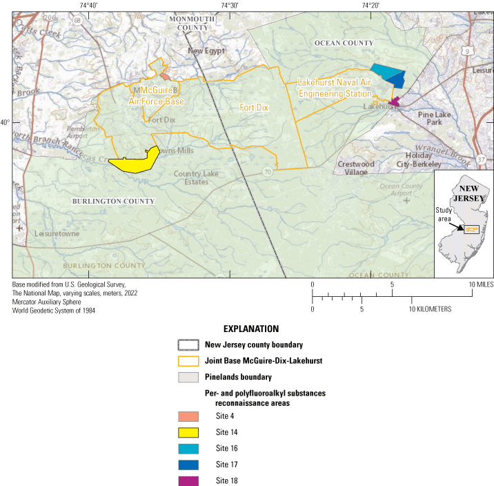
Map showing locations of Joint Base McGuire-Dix-Lakehurst and per- and polyfluoroalkyl substances reconnaissance areas within the New Jersey Pinelands Reserve, Burlington and Ocean Counties, New Jersey.
Purpose and Scope
This report describes development and calibration of a numerical model that simulates regional groundwater flow and advective transport of PFAS in shallow Coastal Plain aquifers underlying JBMDL and vicinity. The flow model, based on the hydrostratigraphic framework of the area developed by Fiore (2020), was calibrated using groundwater level observations and estimated base flows from low-flow stream discharge measurements. The model was used to identify streams and other areas potentially affected by PFAS contamination based on forward particle-tracking flow paths from known PFAS source areas. Reverse particle tracking away from PFAS reconnaissance areas that contain domestic wells potentially contaminated with PFAS was used to identify additional potential sources of PFAS. For the purposes of this study, it was assumed that all reconnaissance areas are contaminated with PFAS throughout their extent.
Previous Investigations and Modeling Studies
The USGS previously developed numerous regional groundwater flow models that encompass parts or all of the study area and rely on the hydrogeologic framework of the New Jersey Coastal Plain described by Zapecza (1989). They include the transient, three-dimensional, multilayered New Jersey Coastal Plain Regional Aquifer-System Analysis (RASA) model (Martin, 1998) and its modifications (Voronin, 2004), as well as groundwater flow models previously developed for the Rancocas Creek watershed (Modica, 1996) and the Toms River watershed (Nicholson and Watt, 1997). Charles and Nicholson (2012) developed groundwater flow models to evaluate effects of groundwater withdrawals on base flow and water levels in parts of the Pinelands National Preserve, in which JBMDL is located. A groundwater model of Ocean County was also constructed to evaluate groundwater supply scenarios (Cauller and others, 2016). Each of these previously developed models either did not cover the entirety of JBMDL or lacked the resolution necessary to make reliable predictions of PFAS advective transport at JBMDL
Site-wide potentiometric surface maps for JBMDL have been developed by contractors (AECOM, 2010; Aerostar, S.E.S., LLC, 2017; and Tehama LLC, 2020). The USGS also collected and analyzed groundwater levels around AFFF source area 14 on Fort Dix (Fiore, 2016) and in a small area of Lakehurst where no AFFF was suspected to be used (Jacobsen, 2000). Each of these assessments did not incorporate numerical modeling into determining the associated groundwater flow directions.
Well Numbering System
In this report, wells are named using a unique numbering system consisting of a numerical two-digit county code followed by a four-digit inventory sequence number. The county codes used are 05, Burlington County; 25, Monmouth County; and 29, Ocean County. For example, well 290139 is the 139th well inventoried in Ocean County. All wells in which water levels were measured by USGS are identified using this nomenclature. Wells on JBMDL for which water levels were measured and reported by the AFCEC contractor, but which have not been visited by USGS, were not given a unique identifier and are designated by name, well depth, location, and elevation information supplied to USGS by the contractor. Well information reported by the contractor is available in the model archive data release associated with this report (Fiore and Colarullo, 2023).
Description of Study Area
The JBMDL spans a nearly 66 square-mile area in Burlington and Ocean counties (fig. 1). Fort Dix makes up the largest of the JBMDL installations in terms of area (about 48 square miles), with a large part of Fort Dix consisting of undeveloped forested areas. Municipalities in the vicinity of JBMDL include Springfield Township, North Hanover Township, New Hanover Township, Wrightstown Borough, and Pemberton Township in Burlington County; and Plumsted Township, Jackson Township, Lakehurst Borough, and Manchester Township in Ocean County. The JBMDL is also within the Pinelands National Preserve (fig. 1), for which heightened environmental protections are required for the region’s water and ecological resources (New Jersey Pinelands Commission, 2022).
Regional Hydrostratigraphic Framework
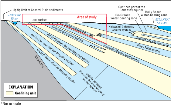
The New Jersey Coastal Plain is underlain by unconsolidated marine and marginal-marine sediments that strike approximately southwest-northeast and dip and thicken to the southeast (Zapecza, 1989) (figs. 2 and 3; table 1). Most of JBMDL is within the outcrop area of the sand, silt, clay, and gravel sequences of the Miocene-age Cohansey Formation and Kirkwood Formation, which together form the Kirkwood-Cohansey aquifer system (fig. 2). Parts of the Eocene-age silts and clays of the Manasquan Formation and the Paleocene-age glauconitic quartz sands of the Vincentown Formation also crop out within JBMDL boundaries. The Manasquan Formation makes up part of the Manasquan-Shark River confining unit that underlies the Kirkwood-Cohansey aquifer system. The Vincentown Formation is categorized as its own aquifer (the Vincentown aquifer), which is confined by the Manasquan-Shark River confining unit. Further description of these hydrogeologic units is discussed in Fiore (2020).
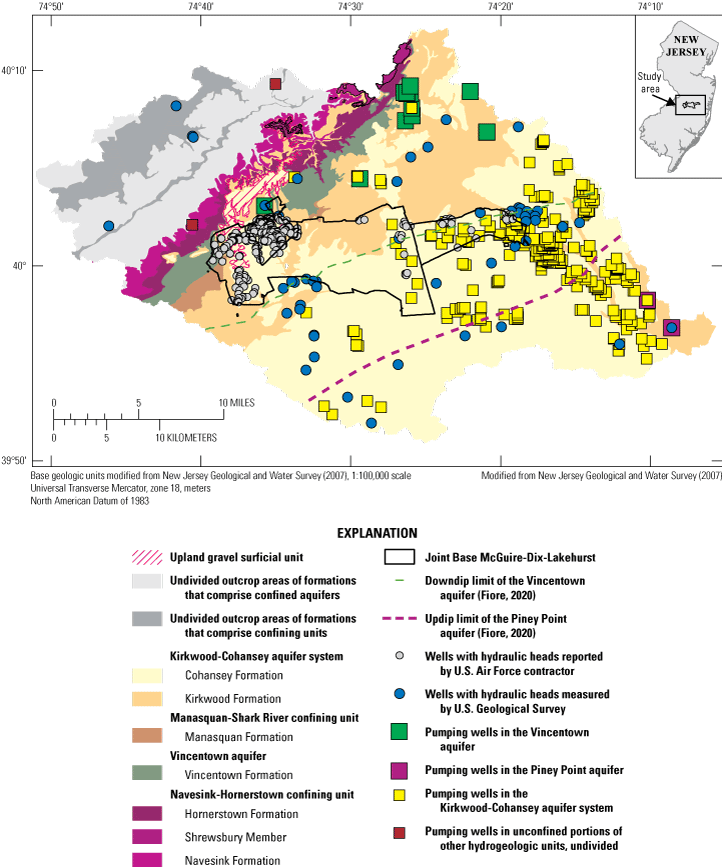
Map of geologic units and location of wells, Joint Base McGuire-Dix-Lakehurst and vicinity, New Jersey.
Conceptual cross section of hydrogeologic units of the New Jersey Coastal Plain. Modified from Gordon and others (2021).
Table 1.
Stratigraphic relations between selected hydrogeologic units and geologic formations in the vicinity of Joint Base McGuire-Dix-Lakehurst, New Jersey. Modified from Fiore (2020).The hydrostratigraphy of JBMDL and vicinity developed by Fiore (2020) formed the basis of the model layer framework used in this study. Fiore (2020) mapped the Kirkwood-Cohansey aquifer system, areas of regionally extensive low permeability sub-units within the aquifer system, the Manasquan-Shark River confining unit, the unconfined and confined portions of the Vincentown aquifer, the Piney Point aquifer, and the Navesink-Hornerstown confining unit.
The Kirkwood-Cohansey aquifer system, the largest unconfined aquifer at JBMDL, is composed of sequences of sands, silts, and clays. Although the aquifer system is largely unconfined, lagoonal back-bay depositional sequences containing silt and clay create discontinuous, low permeability subunits that can produce perched water tables and semi-confined conditions within the aquifer system (Zapecza, 1989). The presence of at least six of these subunits have been identified in and near JBMDL at the regional scale (Fiore, 2020), but their exact configuration and effect on groundwater flow system heterogeneity has not been evaluated. Each of these subunits represents a heterogeneous series of multiple undivided and undifferentiated sand-clay facies (Stanford, 2013; Stanford, 2020), rather than a subunit with consistent hydrolithologic properties. Subsequent geologic mapping by Sugarman and others (2021) indicates the northernmost of these subunits identified by Fiore (2020) is more likely part of the Manasquan-Shark River confining unit, rather than a separate zone within the Kirkwood-Cohansey aquifer system, so is not represented as such in this study.
The Vincentown aquifer is unconfined in its outcrop area, where it receives direct recharge from land surface, as well as where the overlying Manasquan-Shark River confining unit is thin or absent and the Vincentown aquifer has hydraulic connection with the Kirkwood-Cohansey aquifer system (Fiore, 2020). In these instances, the unconfined portion of the Vincentown aquifer and the overlying Kirkwood-Cohansey behave as a single unconfined aquifer and were mapped as such by Fiore (2020). As the thickness of the Manasquan-Shark River confining unit increases downdip toward the southeast, the Vincentown aquifer becomes confined (Fiore, 2020). Farther downdip, the Vincentown Formation grades to finer-grained sediments and its hydrolithologic properties become similar to those of the overlying Manasquan-Shark River confining unit and the underlying Navesink-Hornerstown confining unit that outcrops northwest of JBMDL. Here, the three hydrogeologic units become a single, composite confining unit (Fiore, 2020).
Because both the Kirkwood-Cohansey aquifer system and Vincentown aquifer receive recharge within JBMDL boundaries, both aquifers are also vulnerable to PFAS contamination from JBMDL sources. Domestic wells in the New Jersey Coastal Plain, such as those located in the reconnaissance areas bordering JBMDL, are more likely to be screened to shallower depths than municipal public supply wells, which are more likely to be screened in deeper confined aquifers, which are less vulnerable to PFAS contamination. At PFAS reconnaissance area 4, the Kirkwood-Cohansey is very thin, and the Vincentown is likely unconfined (Fiore, 2020), so domestic wells would more likely be screened in the Vincentown aquifer or the confined Wenonah-Mount Laurel aquifer underlying the Navesink-Hornerstown confining unit, which are themselves relatively shallow at this location. Domestic wells in PFAS reconnaissance areas 16, 17, and 18 are more likely to be screened in the Kirkwood-Cohansey aquifer system because of the increase in thickness of the Kirkwood-Cohansey that occurs downdip, which is in excess of 100 feet (ft) at some locations. Reconnaissance areas 14 and 16 are both near the downdip limits of the confined portion of the Vincentown aquifer, so may include domestic wells completed in that aquifer.
The confined Piney Point aquifer is also included in this study area. The updip limit of the Piney Point aquifer is to the southeast of JBMDL and southeast of the downdip limit of the Vincentown aquifer (fig. 3), and the Piney Point aquifer does not directly underlie the base. The Piney Point aquifer does not crop out at land surface but receives recharge from the Kirkwood-Cohansey aquifer system (Cauller and others, 2016). The Piney Point aquifer is within the Shark River Formation and is stratigraphically higher than the Vincentown aquifer; however, because of the thickening of the Kirkwood-Cohansey and underlying confining unit in the downdip direction, the Piney Point aquifer lies deeper below land surface and thus is less susceptible to PFAS contamination from JBMDL sources (Fiore, 2020).
The hydrostratigraphic framework of Fiore (2020) did not include the confined aquifers and confining units whose recharge areas are updip of the Navesink-Hornerstown confining unit, such as the Wenonah-Mount Laurel aquifer. These aquifers do not crop out within JBMDL boundaries, so are unlikely to receive infiltration from land surface within JBMDL boundaries. For the purposes of the model in this report where the unconfined groundwater flow system must be simulated throughout the study area, the outcropping hydrogeologic units updip of the Navesink-Hornerstown confining unit are assumed to behave as a single, undifferentiated unconfined aquifer down to a depth of 55 ft, an arbitrarily-chosen depth assumed to contain those parts of the aquifers in their outcrop areas plus the overlying younger surficial sediments.
Late Miocene and younger surficial deposits overlie the older Coastal Plain formations that form the aquifers of the study area. These deposits are generally under water-table conditions and are considered to be part of the hydrogeologic unit over which they reside (Fiore, 2020). A notable surficial deposit in the JBMDL area includes upland gravels deposited during sea-level declines in the late Miocene and early Pliocene, and again in the Pliocene and early Pleistocene (Stanford, 2013; Stanford, 2020). The upland gravels form many of the topographic highs in the area, such as the drainage divide between the Delaware River and Toms River. The sand and gravel sediments in the upland gravel are commonly cemented by iron oxide minerals, which can cause perched water tables to form and consequently prevent downward flow of groundwater from the upland gravels into the aquifers that lie below.
Data Sources
Synoptic measurements of water levels in wells collected jointly by USGS and contractors of AFCEC from May 7-11, 2018, formed the dataset for groundwater head observations used in development of the model. Water levels in the Kirkwood-Cohansey aquifer system and Vincentown aquifer were the principal focus of this data-collection effort. In total, water levels in 544 wells were used as head observations in the model. Water levels measured by contractors in 481 wells on JBMDL (Tehama LLC, 2020) are available in a USGS data release (Fiore and Colarullo, 2023). Water levels for additional wells were reported by the contractor but were not used in this model owing to the lack of screened interval information at the time of their reporting. Water levels measured by USGS personnel in 59 wells outside JBMDL boundaries are available in the USGS National Water Information System (NWIS) database (U.S. Geological Survey, 2022) and in Fiore and Colarullo (2023). Most wells on JBMDL were monitoring wells; off-base wells were mostly domestic wells, but also included irrigation, public supply, industrial, and monitoring wells. An additional 4 wells on JBMDL are continuously monitored with pressure transducers by the USGS and were not measured by the contractors. The water levels in these wells that were used in the model were the values recorded on May 9, 2018, at 12 p.m. (12 noon), which represents the midpoint of the synoptic data-collection event.
Water-level data collected by the USGS at additional wells, at different time periods and for purposes unrelated to this study, also were incorporated into the model. Water levels in wells 290116 and 291999, which are screened in the confined Piney Point aquifer within the study area, were measured in November 2008 and November 2018, respectively. Water levels were measured in three wells in the unconfined outcrop area of the Englishtown aquifer system to the west of JBMDL, where the Kirkwood-Cohansey and Vincentown aquifers are not present: 051507 in April 2004, 051481 in May 2018, and 051886 in July 2018. An August 2012 measurement in well 051505, which is in the outcrop area of the Merchantville-Woodbury confining unit west of the Englishtown aquifer system outcrop area, was also included in the model. These measurements helped to constrain the model calibration by providing water levels in unconfined portions of hydrogeologic units that were not measured during the synoptic event.
Well pumping data from the New Jersey Water Transfer Data Model (NJWaTr) (New Jersey Geological and Water Survey, 2018) was also used in the model. Within the study area, data from 375 wells in the Kirkwood-Cohansey aquifer system, 16 wells in the Vincentown aquifer, 4 wells in the Piney Point aquifer, and 2 wells from unconfined outcrop areas of other hydrogeologic units were included in the model (fig. 2). For each well, the average pumping rate from 2008 through 2018 was used. This database contained reported pumpage for public-supply, irrigation, industrial, mining, and commercial wells. Domestic well pumping is not reported in NJWaTr, so is excluded from the model. Areas with domestic-well pumping also tend to have septic tanks rather than municipal sewers, but it was assumed that inputs of water into the unconfined aquifer system from septic tanks balances the outputs from the domestic well pumping at the regional scale of the model. Well-pumpage data are also available in the model data release (Fiore and Colarullo, 2023). Most reported pumping from unconfined aquifers is for wells near the eastern side of JBMDL. On the western side of the base, the Kirkwood-Cohansey and Vincentown are very shallow (Fiore, 2020), so most non-domestic pumping is from wells completed in deeper, confined aquifers.
Base flows were estimated for 20 streams in the study area (fig. 4) using the Maintenance of Variance Extension Type 1 (MOVE.1), based on observed low flows at streamgaging stations draining hydrologically similar sites with at least 10 years of record using regression in R (Colarullo and others, 2018). Base-flow estimates for 11 sites came from existing data in NWIS, but additional low-flow measurements were collected throughout 2018 at 9 additional sites in the study area to obtain a more robust base-flow estimate. All stream discharge data are available in NWIS. Catchment areas for each base-flow measurement were delineated by the ArcGIS Watershed toolset (Esri, 2022).
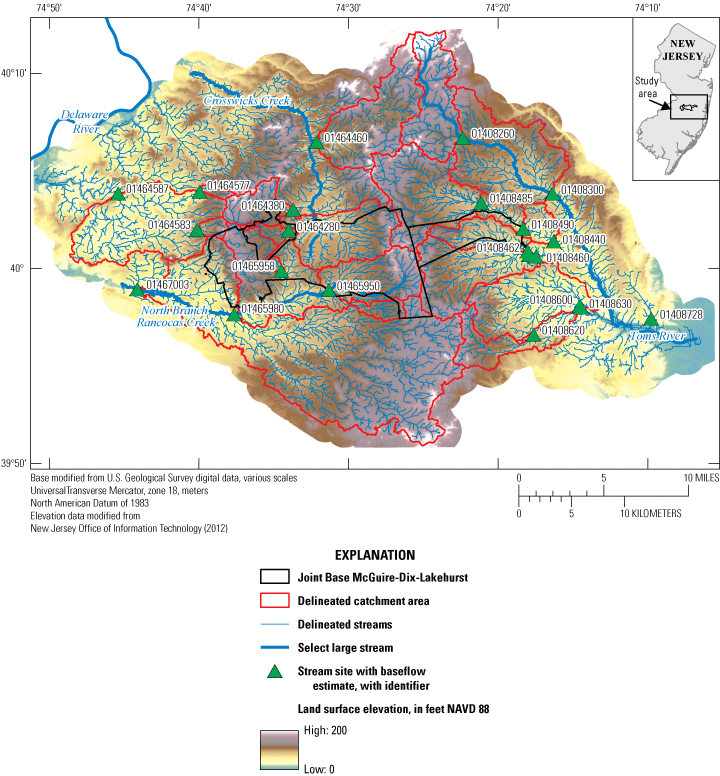
Map of land-surface elevation, stream sites with base-flow estimates, delineated streams, and delineated catchment areas, Joint Base McGuire-Dix-Lakehurst and vicinity, New Jersey.
Simulation of Regional Groundwater Flow
A three-dimensional steady-state groundwater flow model was developed to predict the fate and transport of PFAS dissolved in groundwater beneath JBMDL. Groundwater flow in the unconsolidated Coastal Plain aquifers underlying JBMDL was simulated using the numerical flow model MODFLOW 6 (Langevin and others, 2017). Model input and parameter estimation (PEST) calibration files were created using ModelMuse version 5 (Winston, 2019; Winston, 2022).
Conceptual Groundwater Flow Model
Effective precipitation recharge is the net amount of precipitation that moves through soils and the unsaturated zone into saturated portions of porous media aquifers, after abstractions like evapotranspiration and soil retention storage within the unsaturated zone are accounted for. Given that effective precipitation recharge is the single largest source of water entering the subsurface in this area, it represents an important mechanism driving advective transport of dissolved contaminants from the surface, through the subsurface, and potentially into water supply wells. Regional flows are generally characterized by long, deep flow paths with significant vertical components. Upward regional flow from deep hydrogeologic units into the shallower units in the JBMDL study area represent an additional influx of water into the groundwater system.
Regional subsurface flow beneath JBMDL is characterized by a local groundwater divide that separates eastward flowing groundwater draining into Toms River, which ultimately discharges into Barnegat Bay, from westward flowing groundwater that drains into the North Branch Rancocas Creek and eventually discharges into the Delaware River (fig. 4). Lateral boundaries of the model delineated along topographic divides are assumed to act as natural no-flow boundaries. Under unconfined flow conditions prevailing in shallow aquifers, the topographic divide closely aligns with the groundwater divide along which no groundwater flows laterally into or out of the model.
The single largest component of outflow from the conceptual model is base flow to streams and hydrologically connected wetlands, which act as drains that remove groundwater from the subsurface flow system, quickly conveying it out of the system through the surface-water drainage network. Along these streams, the water table is shallow and commonly intersects the land surface along stream channel bottoms. Smaller quantities of outflow occur as downward regional fluxes into deeper hydrogeologic units, and minor amounts of water are withdrawn from the subsurface through wells for public and domestic supply, irrigation, and other uses.
The conceptual model used as the basis for the three-dimensional steady-state groundwater flow model provided the foundation for developing a groundwater flow model able to account for all major hydrologic processes known to affect subsurface flow driving advective transport of dissolved contaminants beneath the JBMDL.
Delineation of the Lateral No-Flow Boundary
The active flow area is enclosed by the topographic divide, which in the absence of significant withdrawals at wells, generally aligns with the groundwater divide under conditions of unconfined flow. Along this divide, vertically recharging water diverges to produce a boundary that effectively acts as a no-flow boundary. Figure 4 shows the natural no-flow boundary that encompasses the JBMDL, as defined by the topographic divide of the catchment areas. Within this boundary, all precipitation recharging to the subsurface flows into streams that drain either eastward into Barnegat Bay, or westward into the Delaware River. Esri Hydrology tools (Esri, 2022) were used to delineate the location of the divide using a 10-ft LiDAR digital elevation model (DEM) (New Jersey Office of Information Technology, Office of Geographic Information Systems, 2012). By assigning no-flow conditions along the topographic (and groundwater) divide, all cells located outside of the divide were excluded from the model. The active area of the flow model defined by the topographic divide encompasses approximately 1,340 square kilometers (km2) (518 mi2) of the Coastal Plain, bound by the Crosswicks Creek watershed in the north, the Toms River watershed in the east, the North Branch Rancocas Creek watershed in the south, and the Delaware River in the west (fig. 4).
Spatial Discretization
To build a flow model able to accurately account for both horizontal and vertical hydraulic gradients that drive the transport of dissolved PFAS through the subsurface, the grid was refined along both the horizontal and vertical dimensions to more accurately reproduce those gradients. Horizontal refinement focused on increasing spatial resolution in the AFFF source areas, the PFAS reconnaissance areas, and along streams (fig. 5). To discretize the model in the vertical dimension, top and bottom elevations of hydrogeologic units from the previously developed hydrostratigraphic framework (Fiore, 2020) were used for model layer elevation definitions.
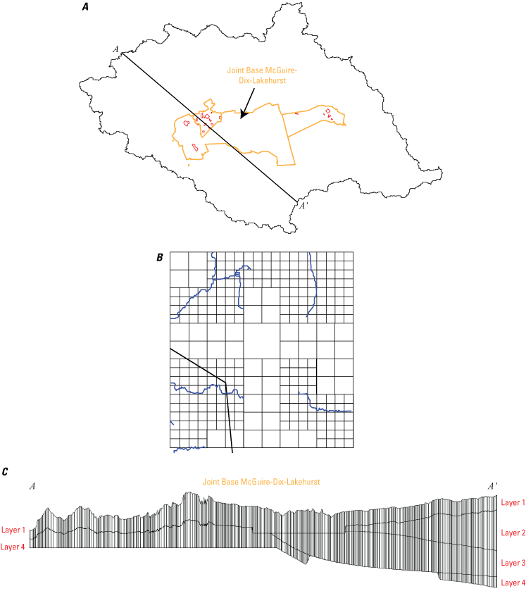
Screenshots showing, A, location of model layer cross section A-A' in study area, B, quadtree grid refinement around select streams, C, model layer cross section A-A', Joint Base McGuire-Dix-Lakehurst and vicinity, New Jersey.
Horizontal Discretization
A principal benefit of using MODFLOW 6 is the ability to locally refine the horizontal grid in areas where greater prediction accuracy is required, without the need to extend fine grid spacings to the edge of the model grid or use slowly converging nested grid refinement algorithms. Because MODFLOW 6 does not support use of both nested and quadtree grids in the same model, quadtree grid refinement was used. These grids, which represent tree data structures for which each parent cell has exactly four child cells, were used to refine the parent grid in areas where preservation of horizontal hydraulic gradients is critical to accurately predicting advective movement of dissolved PFAS. Using a quadtree level of 4, and a grid smoothing operation that adjusts cell size so that no cell shares an interface with more than two adjacent cells (Langevin and others, 2017), quadtree grid refinement of the parent grid produced square cells ranging in size from 125 ft x 125 ft in refined portions of the grid to 1,000 ft x 1,000 ft in areas far from locations where grid refinement occurs, with 250 ft x 250 ft and 500 ft x 500 ft intermediate cell sizes (fig. 5).
Quadtree grids were imposed both inside rectilinear and along curvilinear features (fig. 5). These grids were used to refine the parent grid within polygons representing the five PFAS reconnaissance areas and within multiple known AFFF source areas. The reconnaissance areas represent neighborhoods outside but adjacent to JBMDL boundaries on domestic wells and are considered to be at elevated risk for contamination. Source areas account for locations where known or suspected historical use of AFFF may have released PFAS into the environment. In addition to allowing for local increased spatial resolution in the critical reconnaissance and source areas, MODFLOW 6 enabled creation of quadtree grids along streams to more accurately account for hydraulic gradients adjacent to base-flow-dominated streams in the Coastal Plain and enhance the reliability of predicted base flows.
Vertical Discretization
Following delineation of the lateral no-flow boundary and local horizontal refinement of the three-dimensional grid, vertical layering was introduced by incorporating the hydrostratigraphic framework into the model (fig. 5). Discretization along the vertical dimension was achieved by importing top and bottom elevations of four layers based on the structure of hydrostratigraphic units defined in Fiore (2020). The Kirkwood-Cohansey aquifer system, Manasquan-Shark River confining unit, Piney Point aquifer, Vincentown aquifer, updip, shallow portions of the Navesink-Hornerstown confining unit, and undivided shallow aquifers and confining units lower in stratigraphy were represented across the four model layers. In addition, an upland gravel surficial unit that likely affects groundwater flow in the western part of JBMDL was also represented in the model. For further information about specific layers, see appendix 1.
Introduction of layer top and bottom elevations provided the basis for assigning depths to drain cells and apportioning supply-well withdrawals to layers intersected by specified screened intervals, making it possible to accurately specify internal boundary conditions. The four aquifer layers, which can further be refined using sublayering to better resolve steep vertical hydraulic gradients, impose known hydrogeologic structure on the model and allow aquifer properties unique to each layer, such as hydraulic conductivity (K), porosity, and chemical retardation factors, to be specified. As summarized in table 2, the four layers contain a total of 15 K zones, within which K and other aquifer properties are treated as uniform. Details of the K distribution are discussed later in this report.
Table 2.
Hydrostratigraphic units, model layers, and hydraulic conductivity zones parameter names, Joint Base McGuire-Dix-Lakehurst and vicinity, New Jersey.In addition to varying in thickness across the model area, layers taper out to zero thickness at sedimentary sequence boundaries or geologic unconformities that vary in location with each layer. These boundaries cause discontinuities in the spatial extent of layers, generally referred to as pinchouts. Pinchouts are pervasive throughout the Coastal Plain aquifers that underlie JBMDL. In addition to allowing for local grid refinement, MODFLOW 6 supports use of unstructured grids to incorporate geologic pinchouts. Unlike the structured grid archetype supported by earlier versions of MODFLOW, which requires a fixed number of finite-difference connections for every model cell, an unstructured grid has an arbitrary number of connections to neighboring cells. One benefit of allowing for an arbitrary number of connections to each cell is that the model can include no lateral connections along the edges of pinched-out geologic layers. Although this produces an unbanded, non-symmetric solution matrix that requires a sparse matrix solver, it also makes it possible to design model grids with truncated layers (Langevin and others, 2017). In this MODFLOW 6 model of JBMDL and vicinity, cells in which a geologic layer pinches out were assigned top and bottom elevations of the layer equal to one another to obtain a layer thickness of zero.
Hydraulic Conductivity and Anisotropy
The scale-dependence of hydraulic conductivity (K) and the difficulty of measuring K in situ make the values for this property the most uncertain of model parameters. A unique K zone was delineated for each of the distinct hydrogeologic units influencing groundwater flow in the vicinity of JBMDL. Initial values were systematically varied in PEST calibration runs until optimal sets of horizontal and vertical conductivities were identified by minimizing the sum of weighted squared differences between predicted and observed heads and base flows. A total of 15 K zones were delineated. Within each of the K zones, K in the horizontal directions (x and y) were assumed to be equal. The degree of horizontal to vertical anisotropy (Kxy to Kz) varied among the 15 K zones, but was constant within a K zone. The K zones are described conceptually below and are illustrated on figure 6. Values of K used in the model as determined by PEST calibration are discussed in the Model Parameters section.
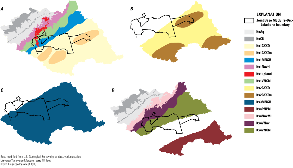
Maps showing hydraulic conductivity zones simulated in groundwater model in, A, layer 1, B, layer 2, C, layer 3, and D, Layer 4, Joint Base McGuire-Dix-Lakehurst and vicinity, New Jersey.
Model layer 1 contains 8 K zones: (1) Kirkwood-Cohansey aquifer system (Kx1CKKD); (2) Kirkwood-Cohansey aquifer system where Fiore (2020) identified a greater prevalence of clay subunits (Kx1CKKDc); (3) a notable upland gravel surficial deposit along the western border of JBMDL (Kx1upland); (4) the outcrop area of the Manasquan-Shark River confining unit where its thickness is less than 28 ft, overlying Kirkwood-Cohansey aquifer system sediments, and overlying surficial sediments (Kx1MNSR); (5) the outcrop area and unconfined portion of the Vincentown aquifer (Kx1VNCN); (6) the outcrop area of the Navesink-Hornerstown confining unit, with overlying surficial sediments (Kx1NavH); (7) undivided western confined aquifer outcrop areas with overlying surficial sediments (KxAq); and (8) undivided western confining unit outcrop areas with overlying surficial sediments (KxCU). The 28-ft thickness of the Manasquan-Shark River confining unit used for Kx1MNSR is based on the thickness estimated by Fiore (2020), where the underlying Vincentown aquifer is most likely confined by the Manasquan-Shark River confining unit, but this should be considered a general approximation. KxAq and KxCU occur where layer 1 overlies layer 4, and these K zones extend into layer 4. The location of the upland gravel surficial deposit is based on 1:100,000 scale mapping by New Jersey Geological and Water Survey (2006), but processed so that all LiDAR DEM cells at 150-ft elevation or higher were assigned to Kx1upland.
The hydraulic conductivity in each of the K zones in model layer 1 assumes a vertical anisotropy where K in the vertical direction (Kz) is assumed to be 10 percent (1/10) of K in the horizontal directions (Kx), except for Kx1CKKDc and Kx1upland, for which Kz was 5 percent (1/20) and 1 percent (1/100), respectively, of Kx. The differences of anisotropy ratios are a consequence of the lithologic nature of these units. Clay is not uniformly distributed within the clayey subunits of the Kirkwood-Cohansey aquifer system represented by Kx1CKKDc, but instead these units have a high density of thin clayey beds interlayered with thin sandy beds (Fiore, 2020), which can cause perched water tables (Zapecza, 1989), and which have been mapped as a “clay-sand facies” in the Cohansey Formation (Stanford, 2013; Stanford, 2020). Groundwater in Kx1CKKDc is therefore assumed to have a stronger horizontal flow component compared to vertical flow, thereby representing how groundwater can flow easily through the permeable sandy beds (higher Kx) but will have a more difficult time flowing from one sandy bed to another above or below because of the clayey beds between them (lower Kz) (fig. 7). Upland gravel surficial units represented by Kx1upland create a similar phenomenon. These deposits contain iron oxide-cemented layers (Stanford, 2013; Stanford, 2020) that can also create perched water tables and result in groundwater seepage to small-order tributaries. Reported hydraulic heads from the western part of JBMDL, where the upland gravel is present, are much higher than heads reported in adjacent areas, with a steep hydraulic gradient on the western slope of the upland gravel (Tehama LLC, 2020), which indicates higher heads in this area are likely caused by this upland gravel. The upland gravel is predominantly gravel and sand so would be expected to have high K in general, but iron oxide cementation may be creating a barrier to downward infiltration and cause the water table to build up in the upland gravel itself. Both preliminary manual calibration of Kz for Kx1upland as well as subsequent PEST calibration indicated a smaller Kx/Kz ratio compared to Kx1CKKDc was required to simulate the high groundwater levels in this unit, so a ratio of 1/100 was assumed.
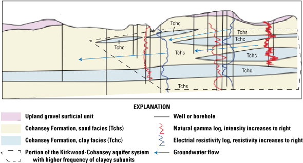
Conceptual cross section of groundwater flow in relation to clayey subunits in the Kirkwood-Cohansey aquifer system. Modified from Stanford (2013).
Model layer 2, which represents deeper portions of the Kirkwood-Cohansey aquifer system, contains 2 K zones similar to the K zones for this aquifer in layer 1: portions of the Kirkwood-Cohansey aquifer system with higher amount of clay subunits (Kx2CKKDc) and portions without (Kx2CKKD). Kx1CKKDc and Kx2CKKDc are not in the same geographic locations in layer 1 and layer 2; the elevations and thicknesses of these subunits from Fiore (2020) determined whether that subunit was included in layer 1 or layer 2, with one subunit spanning both layers. The vertical anisotropy of the zones in layer 2 is assumed to be similar to that in layer 1, with Kz being 5 percent (1/20) of the Kx value for Kx2CKKDc and 10 percent (1/10) for Kx2CKKD.
Model layer 3 contains the deep Manasquan-Shark River confining unit and has only 1 K zone to represent that hydrolithology (Kx3MNSR). Kz was assumed to be 10 percent of Kx.
Model layer 4 contains 6 K zones: (1) the Piney Point aquifer (Kx4PNPN), (2) the confined portion of the Vincentown aquifer (Kx4VNCN), (3) a generalized area below the outcrop area of the Vincentown aquifer that contains mixed Vincentown aquifer and underlying Navesink-Hornerstown confining unit properties (Kx4VNav), (4) a generalized area below the Navesink-Hornerstown confining unit outcrop area that contains mixed Navesink-Hornerstown confining unit and underlying Wenonah-Mount Laurel aquifer properties (Kx4NavML), (5) KxAq, and (6) KxCU. Kz values were assumed to be 10 percent of Kx.
The 15 distinct lithologies incorporated into the model via the four layers provide important qualitative information about the distribution of heterogeneities in the subsurface beneath the JBMDL. This distribution of heterogeneities can have a significant effect on transport of dissolved contaminants through the subsurface, which migrate through interstitial void spaces and can abruptly change direction when heterogeneities are encountered. Even small-scale heterogeneities can substantially alter flow pathlines and dramatically change the location and timing of contaminant travel times. Because measurement of sublayer heterogeneities was beyond the scope of the proposed study, any K variations occurring at a scale smaller than the scale of the regional hydrostratigraphic framework have not been incorporated into the model. These sublayer heterogeneities can profoundly influence subsurface transport of dissolved PFAS beneath JBMDL, and their absence from the model represents a limitation for the particle-tracking component.
Boundary Conditions
Base Flow
Owing to the small topographic relief and low fluvial energy characterizing the Coastal Plain, groundwater contributions to streams are a dominant component of the groundwater budget and represent the single largest sink for groundwater (Charles and Nicholson, 2012).
Streams and wetlands cells in the model were delineated by the NHD-Plus dataset (U.S. Environmental Protection Agency and U.S. Geological Survey, 2012) and base flows were simulated using the MODFLOW 6 drain (DRN) package, which removes groundwater when the elevation of the water table exceeds the elevation of the streambed, conveying it instantaneously out of the groundwater flow system in the form of base-flow contributions to streams at a rate proportional to that elevation difference. The DRN package was applied to model cells along streams and within stream-connected wetlands to simulate the effect of base-flow losses in the base-flow-dominated streams that drain the low-relief Coastal Plain environment.
The DRN package requires inputs of streambed elevation and drain conductance. For streams, the streambed elevation was set to 90 percent of the thickness of the cell in layer 1 above the bottom of layer 1. Wetlands had a streambed elevation equal to the top of the model. Drain conductance is a measure of how easily groundwater seeps through streambed sediments along the sides and bottoms of the streams and hydraulically connected wetlands, where it instantaneously exits the model as base flow. Because drain conductance depends on a wide array of factors, including stream channel shape and bottom sediment thickness, its value is generally one of the most uncertain to specify. A constant conductance value of 5 square feet per day was assigned to streams, and a constant value of 2 square feet per day was assigned to wetlands. Drain conductances can also be estimated by calibration to more effectively reproduce base-flow losses, but these parameters were not chosen as calibration parameters in this model.
Fiore and others (2021) identified losing streams near JBMDL that are associated with dams and weir structures. These losing conditions are not simulated and are assumed to be local to that stream reach, with negligible effect on the regional system. However, low-flow discharge measurements have the potential to be affected by such conditions if a similarly engineered structure exists upstream, which may underestimate base-flow observations for that catchment.
Groundwater Withdrawals
Well pumping, which represents important losses from the flow system, was incorporated into the model using the multi-aquifer well (MAW) package, which can simulate well pumping from screened intervals that span multiple model layers, which is the case for many wells in the Kirkwood-Cohansey aquifer system that pump from layers 1 and 2. However, if a well extended across model layers that were in different hydrogeologic units, for example the Kirkwood-Cohansey aquifer system and the Manasquan-Shark River confining unit, the screened interval was edited to simulate pumping only from the aquifer layer and thus the screened interval in the model may differ from that in NJWaTr and (or) NWIS databases. For settings used for the 387 pumping wells simulated by the MAW package, refer to the model archive data release (Fiore and Colarullo, 2023).
Although losses from groundwater withdrawals within the JBMDL are small relative to base flow losses to streams, the varying rates and depths from which groundwater is pumped impose strong local controls on flow geometry that can fundamentally alter contaminant pathlines. If dissolved contaminants are present anywhere within the capture zones of active water-supply wells, it is likely that the contaminants may be present in the water pumped from those wells.
Recharge
The principal source of water influx to the subsurface flow model is effective precipitation recharge. Effective precipitation recharge is imposed as a boundary condition of type specific flux and represents the single largest source of water to the model. This recharge is what drives flow and advective transport of contaminants through the subsurface. Because its accurate quantification is essential to development of a reliable flow and transport model, recharge is treated as a calibration parameter and allowed to vary freely. Significant uncertainties associated with estimating abstractions from precipitation recharge caused by processes like evaporation and evapotranspiration also necessitate its inclusion as a calibration parameter.
Effective precipitation was incorporated into the model using the recharge (RCH) package of MODFLOW 6. Two generalized recharge zones were defined across the entire top layer of the active flow area to distribute infiltrating recharge through the top boundary of the model. One recharge value was used for wetland area, and another for non-wetland areas (fig. 8). Values for recharge in these zones were estimated by PEST and are described in the “Model Parameters” section of this report.
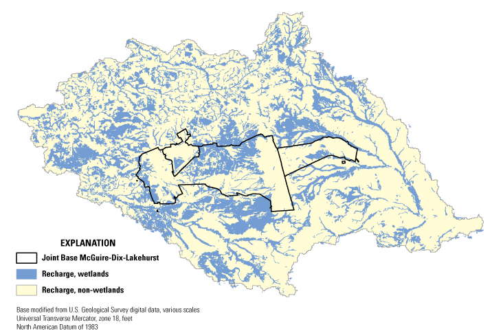
Map showing zones of effective recharge simulated in groundwater flow model of Joint Base McGuire-Dix-Lakehurst and vicinity, New Jersey.
Bottom Fluxes
Along the model bottom, spatially distributed specified fluxes predicted by the RASA regional coastal plain model were assigned as boundary conditions (fig. 9). Specified fluxes along the bottom boundary of the model were assigned based on internal vertical fluxes extracted from the calibrated regional RASA groundwater flow model for the New Jersey Coastal Plain (Voronin, 2004). Although bottom boundary flows represent a small fraction of groundwater losses compared to base-flow losses, they can exert strong controls on the overall mass balance of the flow system. Given the large scale at which they were predicted, however, it is unlikely these fluxes substantially affect local patterns of flow and advective transport near supply wells. Upward influxes and downward outflows across the bottom boundary of the model were incorporated into the model using the well (WEL) package.
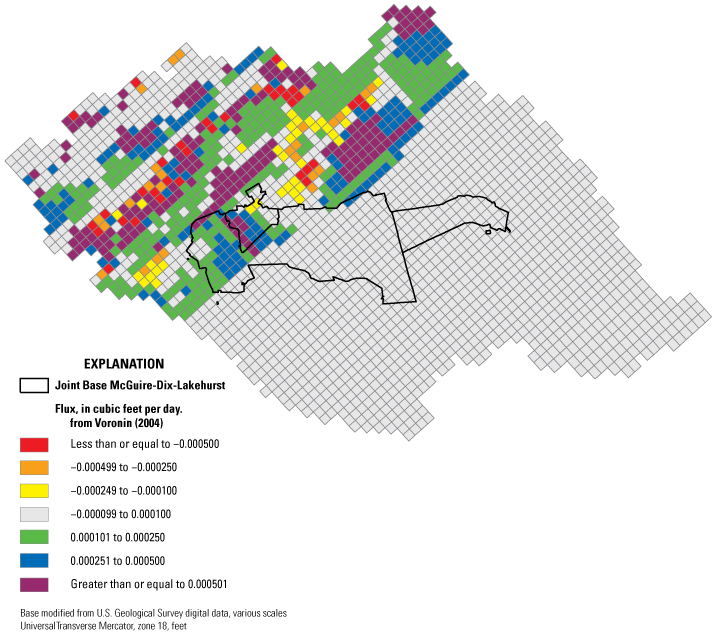
Map showing bottom fluxes from the Regional Aquifer System Analysis (RASA) model (Voronin, 2004) used in groundwater flow model of Joint Base McGuire-Dix-Lakehurst and vicinity, New Jersey. Grid shown is from RASA model.
Model Calibration
Prior to the calibration phase of model development, the steady-state groundwater flow model was tested to ensure that it executed properly in forward mode. The model was then calibrated using PEST, a non-linear model-independent parameter estimation program that relies on gradient search techniques to locate the set of parameters producing the lowest sum of squared weighted residuals (Doherty, 2018). Residuals were defined as the difference between observed heads and base flows and the heads and base flows predicted by the model. Goodness of fit for the calibrated model was assessed by examining various aspects of residuals to determine if statistical or spatial bias was present in the model or if the calibration was influenced by the presence of outlier head or base-flow observations. The PEST calibration was run in “estimation” mode using singular value decomposition (Doherty, 2018).
The PEST program systematically adjusts designated model parameters across their expected ranges until differences between simulated and observed water levels and base flows are globally minimized to within an acceptable convergence tolerance. Optimal parameter values occur at the minimum of the sum-of-squared-weighted-error function over the parameter space. A sensitivity analysis was subsequently performed to determine the degree of model sensitivity to calibration parameters at their optimal values. The PEST program offers multiple options for dealing with issues that can adversely affect calibration of a groundwater flow model. These issues include the presence of correlated parameters that can produce a sum-of-squared-weighted error function characterized by ridges and valleys that can inhibit convergence to a global minimum as well as structural errors in the model that manifest as distributional or spatial bias in calibration residuals.
Model Parameters
The model parameter sets included in PEST calibration are effective precipitation recharge for non-wetland areas (which affects the value for wetland areas, as described below), and horizontal and vertical hydraulic conductivities for the 15 K zones. Stream and wetland drain conductance was not included as a model parameter.
For effective precipitation recharge, the non-wetland area recharge value was the value estimated by PEST, whereas the wetland areas recharge value was assumed, arbitrarily, to be 10 percent of the value estimated for the non-wetland areas by PEST. The optimal recharge estimate for non-wetland areas was 17.1 inches per year, which is characteristic for the New Jersey Coastal Plain (Voronin, 2004). Thus, recharge to wetland areas was assumed to be 1.7 inches per year.
An initial PEST run identified preliminary values and sensitivities for all 15 K zone parameters. This initial PEST run identified 6 K zones that had greater sensitivity—Kx1CKKD, Kx1MNSR, Kx1upland, Kx1VNCN, Kx4VNav, and Kx4VNCN. The other 9 parameters had low sensitivity and were removed from the calibration. When PEST was run again, characteristic Kx values were instead used as constants in the model for these 9 K zones. Kz values were assigned on the basis of the specified anisotropy ratio, as described above. The optimal and constant K values and recharge values used in the model are shown in table 3.
Table 3.
Hydraulic conductivity and recharge values simulated in the model.[Kx, horizontal hydraulic conductivity; Kz, vertical hydraulic conductivity; NA, not applicable; PEST, parameter estimation]
Calibration Observations
The 544 observed water levels and 20 base-flow values were then used as calibration observations for the model. Use of observed base flows, in addition to observed heads, prevented the high degree of correlation between precipitation recharge and hydraulic conductivity parameters from producing a mathematically poorly conditioned calibration problem. Owing to the large magnitudes of estimated base flows relative to observed heads, base-flow observations were “downweighted” relative to head observations so that they would not have a disproportionate effect on the calibration. A description of the weighting process is described in appendix 2. When only observed heads are available for calibration, recharge tends to be directly correlated to hydraulic conductivity parameters and as a result can contribute to an ill-posed calibration problem that yields a non-unique set of optimal parameters. The addition of base flow observations to the calibration dataset helps to avoid this non-uniqueness. Table 4 lists the 20 estimated base flows used in the PEST calibration. Because several of the catchments draining to JBMDL flow sites are nested, PEST calibration was performed using incremental base flows, so the catchments do not overlap for two sites with estimates along the same reach of stream.
Table 4.
Observed and simulated incremental base flows and base flow weights, Joint Base McGuire-Dix-Lakehurst and vicinity, New Jersey.[NWIS, National Water Information System database; cfd, cubic feet per day]
MOVE.1 regression from Colarullo and others (2018).
Residuals
An evaluation of the goodness of fit of the calibrated groundwater model is critical to assessing its utility for accurately predicting the fate and transport of dissolved PFAS in the subsurface. Measures of fit quantify how closely predicted heads and base flows reproduce observed heads and estimated base flows and involve evaluating various properties and behaviors of residuals, defined as the differences between observed and predicted heads and base flows.
Structural error, which generally manifests as a non-diffuse cloud of points in residual plots, may contribute to biased head and base flow predictions (Hill and Tiedeman, 2007). For a model free of structural error, weighted residuals versus weighted observations will plot as a diffuse cloud of points, uniformly scattered above and below the horizontal observation axis, with very little clustering or trending of weighted residuals across the range of weighted observations. The tendency for small-weighted head and base flow residuals to be characterized by a smaller amount of variability around the horizontal axis, often referred to as the proportional effect, occurs when observed heads and estimated base flows are sampled from a log-normal probability distribution (Journel and Huijbregts, 1978). When such observations are log-transformed to perform the regression, but untransformed values are used to assess goodness of fit, this will typically give rise to small variances across smaller ranges of weighted observations and large variances for larger weighted observations. This proportional effect generally contributes small amounts of structural error but can become an important source of systematic error if the lognormal distribution is severely skewed.
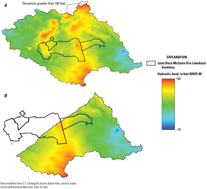
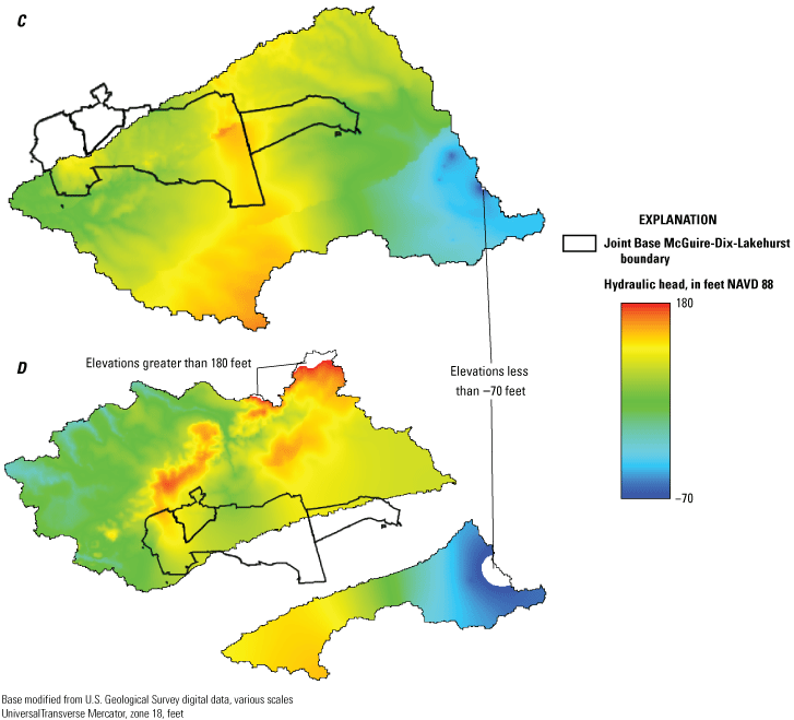
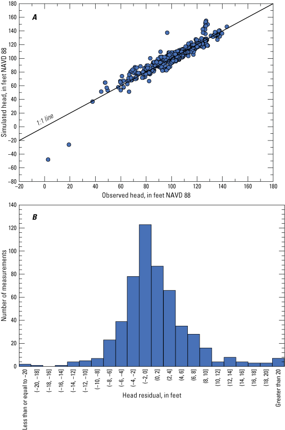
Simulation results indicate that hydraulic heads, and therefore groundwater flow paths, are adequately represented in the calibrated model. Groundwater flow directions indicated by the simulated results (fig. 10A) are consistent with the flow directions indicated by manual contouring of the same observed dataset by Tehama LLC (2020). A histogram of the residuals and the overall fit between the simulated and observed water levels are presented in figure 11, and a map of the residuals in figure 12. Results indicate a generally even distribution of water levels around the 1:1 line on figure 11, with outliers discussed below. The histogram of residuals shows that 210 of the 544 simulated water levels (38.6 percent) are within 2 ft of the observed value, and 502 of the 544 are within 10 ft (92.3 percent) (fig. 11). The model predicts a minor spatial bias in heads (fig. 12), but does not indicate pronounced structural error, as described below.
The largest outliers from the 1:1 line are the 2 water-level observations in the Piney Point aquifer that were not collected during the synoptic event, which have the largest underestimated (negative) residuals of about -50 and -55 ft (fig. 11). These are the only negative residuals greater than -20 ft. The Piney Point aquifer also contains pumping wells, and the model extent of the Piney Point aquifer is too small to represent its hydrologic conditions as more water downdip to the southeast should be available for pumping. Additional outliers (fig. 12) include a cluster of wells along the topographic divide that separates flow between the Atlantic Ocean coastal basins and the Delaware River basins, which have the largest overestimated (positive) residuals and indicate a local spatial bias at this location. Six of the seven wells with a +20 ft residual or greater are in this location, with +41 ft being the largest residual. The other well with greater than +20 ft residual is well 050689 (+21 ft) located on the southern edge of the active model area (fig. 12). Several wells nearby 050689 have residuals between +2 and +10 ft. This part of the active model area was also included in the groundwater flow simulations of Charles and Nicholson (2012), which required more detailed representations than the regional generalizations of this model and indicate a geographic area where the model could use better refinement. Notably, this spatial distribution improves with proximity to JBMDL.
A minor spatial bias is evident on the western portion of JBMDL near AFFF area 15, where a large number of wells have residuals between -2 and -10 ft (fig. 12). AFFF area 15 is a golf course where water is applied as irrigation to the land surface, which may locally increase water levels at that location. In addition, the residuals may be affected by the upland gravel representation at this location. As discussed earlier, perched water tables in that unit, which would cause the large head gradient observed to the western direction, were represented by the low Kz in the vertical direction. If anisotropy here was similar to that in the other units, the groundwater levels in the upland gravel area would instead be underestimated and the radial groundwater high observed in that area would no longer be present. This may create poor representation of the flow paths from AFFF area 15 located on the upland gravel, so this minor spatial bias is an artifact of attempting to more fully represent flow directions at this location. However, this indicates that refinement of the upland gravel units may be necessary for the model and for understanding the unconfined groundwater flow system at JBMDL in general.
Figure 13 shows a plot between observed and simulated base flows. The data cluster around the 1:1 line indicates that base flow is adequately represented in the model. The highest residual occurred for site 01467003, which has the largest drainage area and highest observed base flow, but the residual for this catchment is proportional to its size and attempting to better match this observed base flow may cause a poor match for the other base-flow observations and heads. Also, uncertainties and limitations are inherent with these base-flow estimates that have a more pronounced effect on predicted values for larger drainage areas in the model. Notably, this catchment is also within the Charles and Nicholson (2012) model that contains many of the same wells with residuals of the same range, which further indicates the southern portion of the model could be further refined.
ModelMuse screenshot of simulated hydraulic heads imported from binary head file. A, layer 1, B, layer 2.
ModelMuse screenshot of simulated hydraulic heads imported from binary head file. C, layer 3, and D, layer 4.
Graphs showing, A, plot of observed versus simulated hydraulic heads, and B, histogram of head residuals in the groundwater flow model, Joint Base McGuire-Dix-Lakehurst and vicinity, New Jersey.
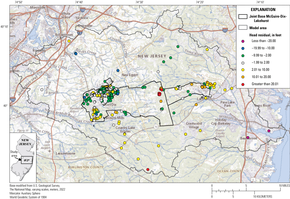
Map showing hydraulic head residuals, Joint Base McGuire-Dix-Lakehurst and vicinity, New Jersey.
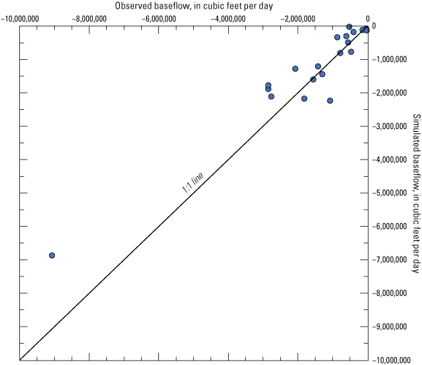
Plot of observed versus simulated base flows, Joint Base McGuire-Dix-Lakehurst and vicinity, New Jersey.
Regional Groundwater Flow Paths and Advective Transport of Per- and Polyfluoroalkyl Substances
The calibrated groundwater flow model provides reliable interstitial flows needed to predict both forward and backward trajectories of dissolved contaminants moving advectively through the subsurface. Applying these flows, MODPATH 7 (Pollock, 2016; Pollock, 2017) particle tracking was used to simulate the pathlines of PFAS emanating from the AFFF source areas, which can then be used to predict which streams, wells, or general locations may be contaminated by PFAS that were not previously considered. MODPATH simulations can also predict the origins of pathlines terminating in the PFAS reconnaissance areas on the borders of JBMDL, which in turn helps to delineate the location and extent of previously unidentified source areas that might pose a risk to downgradient subsurface drinking water supplies under current flow conditions. With both forward and reverse tracking scenarios, no particle tracks entered the Piney Point aquifer nor the aquifers to the west of the outcrop area of the Vincentown aquifer.
Forward Particle Tracking from Aqueous Film Forming Foam (AFFF) Source Areas
AFFF source areas were used as origination points for the MODPATH particle tracks. Initial particle placement in source areas consisted of a 2-by-2 grid of particles placed on the top face of the cell (fig. 14), which represents potential starting points of PFAS at land surface as they enter the groundwater system. Particles were allowed to pass through weak sinks to allow for conservative estimates of potentially affected areas; in other words, particles passing through a weak sink may indicate contamination of both the weak sink as well as the strong sink at which they eventually terminate. This is more useful to assess the full potential extent of the PFAS contamination.
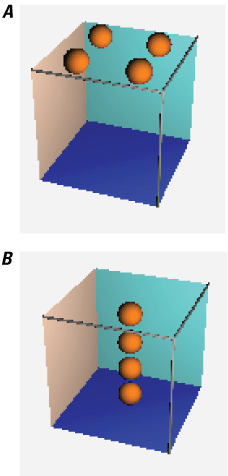
ModelMuse screenshot of diagram showing particle placement within a cell, A, forward tracking scenarios from aqueous film forming foam source areas, and B, reverse tracking from per- and polyfluoroalkyl substances reconnaissance areas, Joint Base McGuire-Dix-Lakehurst and vicinity, New Jersey.
Particles were distributed across the water table within the entire source area polygons; therefore, the particle tracks represent all groundwater flow paths away from these polygons, independent of variability of PFAS concentrations within that source area. Thus, particle tracks emanating from source area polygons may not represent flow paths that contain PFAS if PFAS is not distributed throughout the entire source area. In addition, because any cell that had more than half of its top face area containing a source area polygon was considered an origination point, some particles may begin outside the source area polygon if they are within that same cell. Furthermore, the number of particle tracks originating from source areas is affected by the number of model cells contained in that source area, rather than by the concentration of PFAS within the cells. Thus, a geographically large source area that contains many model cells will have more particle tracks than will a small source area with fewer cells, which causes the particle track results from the larger source area to visually appear more pronounced in the model even if PFAS concentrations from the larger source area are less than those from the smaller source area.
Some parts of JBMDL, in particular McGuire Air Force Base, which has the densest development of buildings and infrastructure of the three installations, have stormwater systems that direct streamflow in culverts that are buried in the subsurface. Information on the locations of these culverts and whether they are designed to hold runoff only or allow exchange with the groundwater was not provided to USGS. The DEM processing method assumed connections of these drainages based on topography that may not accurately represent their connections. The DEM-identified drainages corresponded well to the drainages shown in the immediate vicinity of AFFF source areas at finer, local scale (Aerostar, S.E.S., LLC, 2017), but connections between these features are less confident. The model simulates these features with the DRN package; thus, they receive groundwater discharge and will be termination points of particle tracks. If these engineered drainage features in reality contain only runoff, the particle tracks would not discharge and instead continue downgradient.
Particle tracks from AFFF areas 1 to 15 on McGuire Air Force Base and Fort Dix are shown on plate 1 and tracks from AFFF areas 16 to 21 on Lakehurst Naval Air Engineering Station, are shown on plate 2. None of the particle tracks from AFFF source areas terminate at PFAS reconnaissance areas. Results of particle-tracking scenario from each source area are described below.
AFFF Area 1
AFFF area 1 contains three buildings—Hangar 2251, Building 1708, and Hangar 1837. Particle tracks from Hangar 2251 indicate flow toward the east and northeast and terminate at an unnamed tributary to South Run identified by the DEM (discussed hereafter as “tributary A” to differentiate from other unnamed tributaries in the study area). The location of the DEM-identified drainage portion of tributary A is consistent with the location of an “underground water feature” in Aerostar, S.E.S., LLC (2017). If this drainage receives groundwater discharge, the particle tracks indicate the surface water may be contaminated at this location. If tributary A does not receive groundwater discharge at this location and groundwater continues to disperse downgradient, the effects of other transport properties on PFAS would determine whether downgradient surface water features may be contaminated, the most likely being the main stem of South Run. Tributary A flows into another unnamed tributary of South Run (discussed hereafter as “tributary B”) that flows into the main stem of South Run, The DEM processing has tributary A divided into a northern stem and a southern stem (AFFF area 1 particle flows into the southern stem), but these may actually be part of the same drainage feature.
Particle tracks from Building 1708 and Hangar 1837 indicate groundwater flow to the east. Particle tracks terminate at another unnamed tributary of South Run (discussed hereafter as “tributary C”) that flows into the main stem of South Run downstream of tributary B. Aerial photos (Aerostar, S.E.S., LLC, 2017) indicate tributary C may be an ephemeral drainage; if so, its representation in the model may be overestimated and the eastward flowing PFAS from Building 1708, especially if these are ephemeral drainages that have water levels higher than the water table. The PFAS emanating from Building 1708 and Hangar 1837 may discharge farther to the east if not affected by transport processes. Observed groundwater levels (Tehama LLC, 2020) indicate eastward groundwater flow, but also a northward flow component. Analysis of a surface water sample collected at the confluence of South Run and tributary B had a combined PFOS and PFOA concentration greater than 70 ng/L; it is inconclusive whether this high concentration resulted from flow from Area 1 or from elsewhere at JBMDL.
AFFF Area 2
Particle tracks from AFFF area 2 all indicate eastward flow of groundwater. Particle tracks terminate primarily at South Run unnamed tributary B, with a small number of particles terminating in wetlands near the confluence of tributary B and two other unnamed tributaries to South Run that flow into tributary B (hereafter discussed as “tributary D” and “tributary E”), which indicates surface water at these locations may be contaminated with PFAS if they receive groundwater discharge from area 2. Single particles also terminate in tributary A, Bowkers Run east of the McGuire Air Force Base boundary, and the main stem of South Run. But given the large distance of these indicated flow paths, it is unlikely PFAS originating at area 2 would be detectable at these locations even if infiltration at area 2 discharges there. These portions of tributaries A and C, as well as downstream portions of tributary B, are drainages identified by the DEM processing. If these drainages do not receive groundwater discharge and groundwater continues to flow downgradient, the effects of other transport properties on PFAS would determine whether downgradient surface water features may be contaminated, the most likely being the main stem South Run. Analyses of two water samples collected upgradient of area 2, where tributary B is not contained in a culvert, indicate individual concentrations of PFOA and PFOS that were both less than 10 ng/L (Aerostar, S.E.S., LLC, 2017), which is consistent with the groundwater flow directions indicated by the water levels.
AFFF Area 3
Particle tracks from AFFF area 3 show a predominantly eastward flow and terminate at the northern stem of tributary A. If the drainage feature of tributary A does not receive groundwater discharge as discussed above and is overrepresented as a sink in the model, discharge of groundwater and possible PFAS contamination may occur at the main stem of South Run or downstream portions of tributary B, particularly if PFAS concentrations are higher in the northern portion of area 3. Some particle tracks from area 3 terminate at the western flank of area 3 at tributary B. This is also a feature identified by the DEM processing that does not appear on the NHD nor as a groundwater feature from Aerostar, S.E.S., LLC (2017) so is likely overrepresented in its effects on the hydrologic system. The termination of particles here is likely caused by its proximity to tributary B to the western border of area 3, and hydraulic heads indicate it will more likely flow to the east. Notably, despite the large size of source area 3, particles from this area terminate closer to their point of origin than do particles from source areas.
AFFF Area 4
Particle tracks from AFFF area 4 indicates flow to the southeast. Termination of these particle tracks is at the main stem of South Run, as well as another unnamed tributary to South Run (discussed hereafter as “tributary F”) that flows into the main stem of South Run. Area 4 is small relative to the model cell size that encompasses it, no nearby groundwater levels are available, and no streams are nearby, so at this resolution the flow paths emanating from area 4 are extremely generalized. Only 4 particles were released from area 4. Three of these particles terminate at tributary F, the downstream-most tributary to South Run, which indicates tributary F may be contaminated. The particle that terminates at main stem South Run is a feature identified by the DEM processing that aerial photos (Aerostar, S.E.S., LLC, 2017) indicate may not exist. Thus, this particle likely would terminate downstream at the main stem of South Run.
AFFF Areas 5 and 6
AFFF areas 5 and 6 are discussed together owing to their nearby location in the same wetland area. Particle tracks from these two areas terminate within the surrounding wetland, as well as at tributary E. Because of their location in the wetlands, flow paths in these areas are likely short and shallow, and thus contribute only minor amounts of recharge to groundwater.
Analyses of surface water samples collected from tributary E east of AFFF area 6 indicated that the combined concentrations of PFOA and PFOS exceeded EPA limits (Aerostar, S.E.S., LLC, 2017), which is consistent with particle track results. Tributary D to the north also had a surface water sample with concentrations exceeding EPA limits, but it is inconclusive whether this result is because of the wetlands representation in the model underestimating the flow paths or whether the high concentrations originated from a different PFAS source.
AFFF Area 7
Particle tracks from AFFF area 7 indicate eastward and southeastward flow. All particle tracks terminate at Jacks Run, which flows through area 7. This is consistent with surface water samples from Jacks Run near AFFF area 7 with concentrations that exceeded EPA limits for combined concentrations of PFOA and PFOS (Aerostar, S.E.S., LLC, 2017). Jacks Run eventually flows into Little Pine Lake, in which high concentrations PFAS have been reported by the NJDEP (Goodrow and others, 2018).
AFFF Area 8
Particle tracks from AFFF area 8 terminate to the east at Bowkers Run, which is a tributary to Jacks Run. No surface water samples were collected in Bowkers Run (Aerostar, S.E.S., LLC, 2017), but if PFAS are present in area 8, there is a strong possibility of PFAS contamination of Bowkers Run. Bowkers Run eventually flows into Little Pine Lake, in which high concentrations of PFAS have been reported by the NJDEP (Goodrow and others, 2018).
AFFF Area 9
Particle tracks from AFFF area 9 indicate eastward flow that terminates at Larkins Run, which is a tributary of Jacks Run. A drainage within area 9 was considered by the DEM processing to flow into South Run, but the water actually flows through a culvert under the runway into Larkins Run. This discrepancy is a consequence of the minor variation in topography in the wetlands between the runways where area 9 is located, combined with the elevated runways that the DEM processing believed to be topographic divides that did not account for the engineered structures. In a surface water sample collected from Larkins Run at a more upstream northern reach than where the model indicates discharge to Larkins Run, combined PFOA and PFOS concentration was less than the EPA limit, but individual PFOA and PFOS concentrations both exceeded NJDEP MCLs for those compounds (Aerostar, S.E.S., LLC, 2017). Because particle tracks indicate most discharge occurring at other reaches of Larkins Run than where this sample was collected, concentrations of PFAS that exceed the EPA limit may occur farther downstream in Larkins Run. Alternatively, the PFAS detected in the Larkins Run sample may indicate flow from area 9 may be more toward the northeast than the model indicates. Given the relatively few groundwater levels measured near area 9, the flow paths are not well defined.
AFFF Area 10
Particle tracks from AFFF area 10 terminate in the main stem of South Run, which flows through area 10. Contamination of South Run by PFAS originating in area 10 is consistent with two surface water samples collected at South Run within area 10, which both had concentrations exceeding EPA limits for combined PFOA and PFOS (Aerostar, S.E.S., LLC, 2017).
AFFF Area 11
Particle tracks from AFFF area 11 terminate at the main stem of South Run, and the northern branch of tributary A. A surface water sample was collected from South Run near area 11 with concentrations below EPA limits for combined PFOA and PFOS but above NJDEP MCLs for individual PFOA and PFOS (Aerostar, S.E.S., LLC, 2017). This sample was collected to the east-northeast of area 11, and within the flow paths from area 11. Thus, high PFAS concentrations at South Run at this sampling location likely was caused by sources in area 11.
AFFF Area 12
Particle tracks from AFFF area 12 indicate flow to the east and south, which is consistent with observed water levels. Particle tracks terminate at the unnamed tributary D of South Run that flows through area 12. This is consistent with a surface water sample collected in tributary D within area 12, which exceeded EPA limits for combined PFOA and PFOS (Aerostar, S.E.S., LLC, 2017).
AFFF Area 13
Particle tracks from AFFF area 13 indicate east and northeast flow that terminates at tributary D. This is consistent with a surface water sample collected in tributary D near area 13, which exceeded EPA limits for combined PFOA and PFOS (Aerostar, S.E.S., LLC, 2017).
AFFF Area 14
At AFFF area 14, the discharge of wastewater effluent into the subsurface via infiltration basins causes high hydraulic heads locally depending on which basin is in use (Fiore, 2016). As a consequence, groundwater moves radially away from the infiltration basins, which is consistent with the multiple flow directions indicated by particle tracks simulated by the model. However, the model does not account for the increased infiltration into groundwater associated with this site.
Most particle tracks terminate to the south at Cannon Run and its tributaries, which is consistent with two surface water sample with concentrations exceeding EPA limits for combined PFOA and PFOS (Aerostar, S.E.S., LLC, 2017). Additional particle tracks terminate at an unnamed tributary of North Branch Rancocas Creek to the east of area 14. If infiltration is focused on basins in the northern part of the site, flow may also occur toward Ong Run in the northeast, though no particle tracks terminated at Ong Run in this model. Which basins were in use during the 2018 groundwater level synoptic event was not reported. No samples were collected from the unnamed tributary to North Branch Rancocas Creek nor Ong Run (Aerostar, S.E.S., LLC, 2017), but high PFAS concentrations may be present in those stream locations.
AFFF Area 15
AFFF area 15 covers a large area, and particle tracks indicate multiple flow directions. Tributary D flows through area 15, and many particle tracks terminate in that tributary. Two surface water samples collected in tributary D within area 15 were below the EPA limit for combined PFOA and PFOS concentrations, but above the NJDEP MCL for individual PFOA and PFOS (Aerostar, S.E.S., LLC, 2017). The sampling locations were in the upstream portion of tributary D, and additional particle tracks terminate downstream of the sampling locations, so higher PFAS concentrations may be present in tributary D downstream of the sampling locations depending on where within AFFF area 15 the PFAS concentrations in groundwater are highest.
Substantial flow from area 15 also occurs to the southwest. Both observed and simulated water levels indicate a very steep hydraulic gradient in this direction, which is likely related to the upland gravel surficial deposit that underlies area 15. Particle tracks flowing west predominantly terminate at Indian Run and at unnamed tributaries to Indian Run. No surface water samples were collected in these streams (Aerostar, S.E.S., LLC, 2017), but model results indicate the streams may be contaminated by PFAS originating in area 15.
AFFF Area 16
AFFF area 16 consists of two historical fire training areas (note that AFFF areas 16-21 are on Lakehurst Naval Air Engineering Station and are shown on plate 2). Particle tracks from area 16 indicate groundwater flow to both the west and east and terminate at unnamed tributaries to Manapaqua Branch. The tributary to the west is discussed hereafter as “tributary G” and the tributary to the east “tributary H”. A surface water sample with concentrations that exceeded EPA limits for combined PFOA and PFOS concentrations was collected (Aerostar, S.E.S., LLC, 2017) in tributary G. The elevated concentrations of PFAS in this sample are to be expected with particle tracks terminating upstream of the sampling location. Tributary H is a drainage identified by the DEM processing method. If tributary H is a stream or other drainage feature at which groundwater discharges, particle tracks indicate it may be contaminated with PFAS. If tributary H is a drainage feature that does not receive groundwater discharge, PFAS may flow farther east, and its fate would be determined by effects of other transport processes.
AFFF Area 17
Particle tracks from AFFF area 17 terminate at pumping wells 291329 and 291330, which indicates those wells may be contaminated with PFAS. Wells 291329 and 291330 are listed as industrial-supply wells in the NJWaTr database (New Jersey Geological and Water Survey, 2018). A water sample collected from Ridgeway Branch, near and to the northeast of area 17 contained a combined concentration of PFOA and PFOS that exceeded the EPA limit (Aerostar, S.E.S., LLC, 2017). Although no particle tracks in the model terminate at Ridgeway Branch, it is likely that the PFAS in this sample originated in area 17, but the model may overestimate the effects of the pumping wells on groundwater flow directions near area 17. In addition, if these wells are not continuously in use, the sample may have been collected at a time when the wells were not pumping, a condition that is not represented by the steady-state nature of this simulation. This apparent discrepancy may also be caused by a resolution issue given the small geographic area of AFFF area 17 relative to the regional model cell size, such that heterogeneity is not accurately represented at this location.
AFFF Area 18
Particle tracks from AFFF area 18 indicate eastward flow terminating at unnamed Manapaqua tributary G as well as westward flow terminating at another unnamed tributary to Manapaqua Branch (hereafter discussed as “tributary I”). Eastward particle tracks are consistent with a surface water sample collected along tributary G that contained a combined concentration of PFOS and PFOA that exceeded the EPA limit (Aerostar, S.E.S., LLC, 2017). Given the proximity of particle termination locations at tributaries G and I to the main stem of Manapaqua Branch, it is also possible PFAS may enter Manapaqua Branch from AFFF area 18, but no particle tracks terminate at the main stem in the model. Similarly, pumping well 291227, which is listed as an industrial-supply well in the NJWaTr database (New Jersey Geological and Water Survey, 2018), is also near area 18 and may be vulnerable to PFAS contamination despite the absence of any particle tracks terminating at the well in this steady-state simulation.
AFFF Area 19
Particle tracks from AFFF area 19 indicate northeastward groundwater flow, and termination at Obhonan Ridgeway Branch, which is a tributary of Ridgeway Branch, and surrounding wetlands. A surface water sample was collected that was below the EPA limit for combined PFOA and PFOS concentrations, but above the NJDEP MCL for individual PFOA and PFOS (Aerostar, S.E.S., LLC, 2017). This sample was collected on a small tributary of Obhonan Ridgeway Branch that was not identified by either the NHD dataset or the DEM processing. The particle tracks from area 19 terminate downstream of the sampling location, so PFAS concentrations in Obhonan Ridgeway Branch may be higher downstream of that sampling location. A cluster of particles terminates along runways at a drainage identified by the DEM processing method. This result is likely an artifact of the processing method inaccurately identifying drainages around the runways, similar to AFFF area 9, so these particles will likely continue northeast and discharge at Obhonan Ridgeway Branch.
Some particles also terminate at pumping well 291270 near the northern border of JBMDL, and no particles terminate at pumping well 291126 near the northern boundary of area 19. However, given the steady-state conditions of the simulation, they should be considered vulnerable to contamination by PFAS if transient conditions cause differing hydrologic conditions. These wells are listed as industrial-supply wells in the NJWaTr database (New Jersey Geological and Water Survey, 2018).
AFFF Area 20
AFFF area 20 consists of 3 sites. These include Hangar 690, a helistat crash site directly west of the hangar, and a plane crash site to the south of the hangar. Some particle tracks from Hangar 690 and the helistat crash site terminate at tributaries G and H, downstream of the endpoints of particle tracks from AFFF area 16, which indicates additional PFAS discharges into these tributaries from AFFF area 20. However, Aerostar, S.E.S., LLC (2017) indicates that tributary G is within a culvert where it passes through the helistat crash site, and concentrations of PFAS in a water sample collected on the downstream end of the culvert were less than both EPA and NJDEP limits. This indicates the culvert is not receiving PFAS-contaminated groundwater, either because the culvert is not in hydraulic connection with groundwater or because the groundwater flows underneath the culvert and discharges to the south. The low concentration sample also indicates that the high PFAS concentration detected in the upstream sample from tributary G decreases during the approximately 3,500 ft stretch between the sampling locations, but the exact reason for this decrease is unknown. If the PFAS-contaminated groundwater originating at Hangar 690 and the helistat crash site flows underneath this culvert, it may discharge at tributary I, to another unnamed tributary to Manapaqua Branch (hereafter discussed as “tributary J”), to the main stem of Manapaqua Branch, or may be captured by one of the pumping wells to the south of these sites, such as 291333 at which 3 particles terminated.
Particle tracks from the plane crash site terminate at tributary J and at pumping wells 291331 and 291333, which indicates these locations may be contaminated with PFAS. Tributary J was identified by the DEM processing method but is not included in the NHD, so may not exist, in which case these particle tracks either would terminate at surface water locations farther southwest or be captured by 291331 and (or) 291333, which are industrial-supply wells, according to the NJWaTr database (New Jersey Geological and Water Survey, 2018). If effects of these two wells are overestimated in the simulation, groundwater flow would likely continue toward the south and discharge at the main stem of Manapaqua Branch or downstream on tributary J if transport processes did not lower concentrations over that distance.
AFFF Area 21
Particle tracks from AFFF area 21 indicate a southeastward flow direction and terminate at tributaries G and J. The tributary G discharge locations coincide with the collection site of a sample in which PFAS concentrations exceeded EPA limits for combined PFOA and PFOS, which indicates the contamination present in tributary G may be caused by area 21. These high concentrations, however, could have resulted not only from PFAS sources at area 21, but also from sources at AFFF area 16 that had discharge upstream of the sampling location. Tributary J has not been sampled and, as stated above, may not exist. However, if tributary J is a real drainage feature, it may be contaminated with PFAS given the termination of particles from area 21 as well as area 20 plane crash site.
Reverse Particle Tracking from Per- and Polyfluoroalkyl Substances Reconnaissance Areas
Reverse MODPATH particle tracking scenarios from five PFAS reconnaissance areas were run to assess possible locations of PFAS sources that may affect each of those areas. In the scenarios, four particles are initially arranged vertically, evenly spaced internally through the height of the cell (fig. 14). The reverse, or ‘backward’ tracking capability of MODPATH was then used to identify origination points of the particles that would terminate at those depths within each reconnaissance area, representing areas from which PFAS would originate if found at a hypothetical well screened at that depth at that location. Unlike the forward tracking scenario in which particles begin at the top of layer 1, reverse particle tracking extends through all 4 layers of the model to test where the source areas would be for every aquifer that underlies each reconnaissance area. Additional MODPATH settings and the same limitations regarding spatial extents of each polygon and their effects on the particle track results discussed for the AFFF source areas also apply here. It also is important to note that particle tracks do not imply that the groundwater in that flow path is contaminated with PFAS, or that wells in the reconnaissance areas are contaminated with PFAS; this approach is used only to identify possible source areas for any PFAS that may be detected in the reconnaissance area.
The results of reverse particle scenarios for McGuire Air Force Base and Fort Dix are shown on plate 1, and results for Lakehurst Naval Air Engineering Stations are shown on plate 2. Particle are divided between those that were reversed tracked from the Kirkwood-Cohansey aquifer system and other unconfined aquifers (layers 1 and 2), and those that were reverse tracked from the confined portion of the Vincentown aquifer (layer 4) and terminated at the water table. Particles that were reverse tracked from the confined portion of the Vincentown aquifer and which terminated in the confined portion of that aquifer, in the Piney Point aquifer (layer 4), or in the Manasquan-Shark River confining unit (layer 3) are not shown on plates 1 and 2 because it was assumed that all PFAS enter the groundwater system at the water table. Particles that were reversed tracked from the Manasquan-Shark River confining unit are also not shown on the plates because it was assumed that no domestic wells are screened in the confining unit, which is a valid assumption given their low likelihood to produce water for pumping and that no pumping well used in this model is screened in the Manasquan-Shark River confining unit. Full MODPATH reverse tracking results are available in Fiore and Colarullo (2023). Discussion of reverse particle track results are limited to particles terminating within the boundaries of JBMDL; particles terminating at off-base, non-JBMDL locations are shown on plates 1 and 2, but not discussed.
Reconnaissance Area 4
Particles reverse tracked from reconnaissance area 4 terminate to the southwest. Reconnaissance area 4 is located north of AFFF area 4, which had flow paths to the southeast and is east of the flow paths that intersect reconnaissance area 4. Therefore, model results indicate that any PFAS that may be present in reconnaissance area 4 did not originate at AFFF area 4 and there may be an additional source of PFAS to the west of AFFF area 4 and to the east of AFFF area 3. MODPATH tracking results also show particles reversed tracked from the Vincentown aquifer underlying reconnaissance area 4, indicating that wells in the Vincentown aquifer at this location may be contaminated with PFAS, assuming other transport processes do not affect concentration of the PFAS in groundwater along that flow path. Reconnaissance area 4 is within the unconfined portion of the Vincentown aquifer. Fiore (2020) suggested, on the basis of downward vertical head gradients indicated by continuously monitored water levels, that the unconfined portion of the Vincentown aquifer may be contaminated and that such contamination may be expected when there is no overlying confining unit preventing downward migration of PFAS.
Reconnaissance Area 14
Many particles reverse tracked from reconnaissance area 14 terminated north of AFFF area 14 and south of AFFF area 15. Some particle paths are entirely within the Kirkwood-Cohansey aquifer system, and some that were reversed tracked from the confined portion of the Vincentown aquifer terminated at the water table after having passed through the unconfined portion of the aquifer, represented in the model as locations where thickness of the Manasquan-Shark River confining unit is less than 28 ft, as discussed earlier. These particle tracks may be associated with the representation of the upland gravel in the model, given their starting locations near the edge of the upland gravel. If a PFAS source area occurs in this general location (between AFFF areas 14 and 15), the likelihood of PFAS-contaminated groundwater reaching reconnaissance area 14 would depend on the effects of transport processes on PFAS. However, the similar tracks these particles take indicate these flow paths are regional at this model resolution rather than a specific identification of flow from a PFAS source area, so increased grid refinement would be needed for certainty.
Additional particle tracks in the Kirkwood-Cohansey aquifer system also originate in the vicinity of AFFF area 14. Thus, it is likely that PFAS present in reconnaissance area 14 originates at AFFF area 14, but model resolution is too limited to show a substantial number of reverse particle tracks that leave reconnaissance area 14 terminating in AFFF area 14. Additional particle tracks in the Kirkwood-Cohansey aquifer system originate within reconnaissance area 14 and in adjacent bordering locations, so shallower wells, particularly those near the edge of the reconnaissance area, likely intersect shallower groundwater flow paths compared to those that would emanate from AFFF area 14 or elsewhere. These shallower flow paths indicate that any PFAS in shallow wells may have a different source than AFFF area 14.
Particles reverse tracked from the Vincentown aquifer underlying reconnaissance area 14 that begin on JBMDL indicate that wells completed in the confined portion of the Vincentown aquifer may be contaminated with PFAS, assuming other transport processes do not affect concentration of the PFAS in groundwater along that flow path. However, lower concentrations are likely, considering the long particle flow paths from the outcrop area to the downdip limit of the confined portion of the aquifer.
Reconnaissance Area 16
Particles were reverse tracked from reconnaissance area 16 in both the Kirkwood-Cohansey aquifer system and the Vincentown aquifer.
Kirkwood-Cohansey aquifer system particle tracks in layers 1 and 2 originate southwest of reconnaissance area 16, many of which are north and east of AFFF area 16, which has flow paths to the south. Thus, the model indicates that any PFAS potentially present in reconnaissance area 16 may originate at a source other than AFFF area 16. The particle tracks that leave reconnaissance area 16 span a large adjacent boundary of JBMDL, which increases the likelihood that there may be another source in that location north of AFFF area 16. Many of these particle tracks leaving reconnaissance area 16 terminate in reconnaissance area 16, so if a relatively shallow well is contaminated with PFAS it may have captured water from a shallower flow path from an unknown source area in close proximity.
Some of the Kirkwood-Cohansey aquifer system and all of the Vincentown aquifer particle tracks originate far west from reconnaissance area 16, so any PFAS that flow along this path would likely be affected by other transport processes prior to its arrival, so it is less likely that those areas are contaminated with PFAS in reconnaissance area 16. Similar to reconnaissance area 14, the downdip limit of the Vincentown aquifer runs through reconnaissance area 16, so it is less likely that PFAS sources in its outcrop area would affect groundwater in the confined portion.
Reconnaissance Area 17
MODPATH particle tracking results show only a small number of reverse particle tracks from reconnaissance area 17 that terminate outside the borders of that reconnaissance area. Ridgeway Branch flows along the southwest border of the reconnaissance area, and the lack of particles beginning north of Ridgeway Branch that made it onto JBMDL to the south indicates Ridgeway Branch is acting as a hydrologic divide in the model at this location. It is inconclusive whether these effects of Ridgeway Branch acting as a flow barrier is only represented in the model as such, or whether the stream also provides a flow barrier in nature. Because of the possibly overestimated effect of pumping wells in this area, as evidenced by all forward particle tracks from AFFF area 17 being captured by pumping wells described earlier, the absence of particles terminating at AFFF area 17 are inconclusive.
On the southern edge of reconnaissance area 17, Kirkwood-Cohansey aquifer system flow paths are to the south and terminate along the easternmost border of JBMDL. This result indicates that any PFAS in the Kirkwood-Cohansey aquifer system in that location, if present, may emanate from a location where no AFFF source area has been identified on the easternmost border of JBMDL.
Many particles reverse tracked from reconnaissance area 17 terminated at the water table within reconnaissance area 17, which indicates that if a relatively shallow well within reconnaissance area 17 is contaminated with PFAS, it may have captured a shallower flow path from an unknown source area in close proximity.
Reconnaissance Area 18
Particle tracks that leave reconnaissance area 18 terminate to the west and northwest of that location. The cells where particles are terminating at the water table are more than 1,000 ft east of AFFF area 18, which indicates any PFAS that may be present in reconnaissance area 18 may originate from a source other than AFFF area 18, including similar area along the easternmost border of JBMDL also indicated by reconnaissance area 17 results. No additional AFFF source areas are located in that portion of JBMDL.
Limitations of the Regional Model
Because the JBMDL groundwater flow model was developed primarily to help make decisions about the management of potentially contaminated drinking-water supplies, the known limitations of the model that might adversely impact the reliability of predicted groundwater flow paths should be acknowledged.
Structural error in a model is a systematic error that occurs when important physical processes are either omitted from the model or are not accurately accounted for. In the JBMDL regional flow model, the primary potential source of structural error is the lack of precise information about the locations of small-scale heterogeneities that could have a significant effect on groundwater flow paths. This lack of information includes that of detailed data on the heterogeneities in each of the K zones; while these unknown heterogeneities do influence hydraulic-head and base-flow observations in nature, systematic error in the model may occur unless the heterogeneities are sufficiently small for their effect to “average out.” With each hydrogeologic unit being represented by either one or two model layers and a coarse grid resolution over many parts of the model, these heterogeneities become even more generalized in the simulation.
Although the model simulates hydrologic conditions at steady state, actual conditions are transient, thus varying over time. The synoptic groundwater-level measurement event on JBMDL took place during one week, with some additional off-site water-level measurements made outside that week. The inherent assumption is that during this event, the water levels did not vary enough to affect interpreted groundwater flow directions, but minor variations in recharge, well pumping rates, and other factors may cause variation. In addition, base-flow estimates for streams represented long-term averages rather than the actual base flow occurring at the time of the groundwater level measurements were collected, so the hydrologic conditions during the synoptic groundwater level measurement event may be different from the long-term average conditions.
Groundwater levels reported by U.S. Air Force contractors were collected in wells that have never been visited by USGS personnel. Therefore, well location and construction information such as screened intervals could not be verified. Additionally, the model does not simulate any withdrawals from domestic wells within the study area, which would likely affect hydraulic gradients and flow directions locally. Other local-scale effects on hydrology, such as locations or point-recharge at land application sites or irrigation, are also not included in the simulation.
In the model, surface water is represented by base-flow losses from the groundwater system, but streamflow itself is not simulated. Thus, the fate of PFAS in streams cannot be assessed with this model. In addition, the model assumes all streams are gaining reaches, and that losing reaches such as those identified by Fiore and others (2021) are of only local extent and do not represent regional conditions. However, if local losing reaches affect heads that are used as water-level observations in the model, the groundwater flow paths may be misrepresented. Stream elevations were determined by the Lidar DEM rather than by measuring stream stages. These surface-water unknowns are an area for further refinement that would improve understanding of the entire hydrologic system in the vicinity of JBMDL. In addition, streambed conductances are often a model calibration parameter, but were assumed constant in this model for all streams. Streambed conductance will vary depending on the particular stream, so inclusion of streambed conductance as a calibration parameter may better represent the surface-water system as well as improve match of simulated to observed base-flow values.
The transport of PFAS in the subsurface is affected by several processes such as sorption and diffusion that are not accounted for with advective particle tracking used in this model. Additionally, the particle tracks do not take into account known PFAS concentrations in groundwater, only groundwater flow paths from AFFF source areas and PFAS reconnaissance areas, so the results assume an equal likelihood of PFAS being transported with groundwater from all flow paths regardless of sampling results from wells in the source areas and in wells and streams along the flow path. Particle tracking results also contain travel times for each particle that were not discussed in this report. Travel times are dependent on the effective porosity of the aquifer material, but effective porosity values were not assessed in this study. Thus, travel times computed by MODPATH are uncertain and should not be used to infer travel time of PFAS in the subsurface.
Summary
The contamination of groundwater and surface water by per- and polyfluoroalkyl substances (PFAS) has been detected at Joint Base McGuire-Dix-Lakehurst (JBMDL) and vicinity in New Jersey. These substances are associated primarily with the use of fire-suppressing aqueous film -forming foam (AFFF) at JBMDL. To assess the extent of PFAS contamination and to determine locations of sources that may have contributed to the presence of these substances in the groundwater and surface water, a three-dimensional steady-state MODFLOW 6 groundwater flow model was developed. The unstructured grid capabilities of MODFLOW6 were utilized to “pinch out” model layers in accordance with the structure of the unconsolidated Coastal Plain hydrogeologic units, as well as to refine the model grid around streams, AFFF source areas, and PFAS reconnaissance areas where more detailed groundwater flow paths were desired. The model simulated groundwater flow in the Kirkwood-Cohansey aquifer system, the Manasquan-Shark River confining unit, the Vincentown aquifer, the Piney Point aquifer, and undivided surficial unconfined aquifers in the vicinity of JBMDL.
The MODFLOW 6 model was calibrated using the parameter estimation (PEST) program, based on 544 observed heads that were largely collected during a single synoptic measurement event during the spring of 2018, as well as 20 base flows estimated for streams on the basis of multiple low-flow discharge measurements collected at various periods. PEST identified the set of parameter values occurring at the minimum of the sum-of-squared-weighted-error objective function, using a gradient search algorithm to iteratively search along the surface of the error function. Residuals between observed and simulated heads and base flows indicated an adequate match. Also incorporated into the model were reported well pumping from municipal supply, industrial, commercial, and irrigation wells screened in the aquifers simulated in the model, as well as bottom fluxes extracted from the New Jersey Coastal Plain Regional Aquifer System Analysis model. Of 15 hydraulic conductivity (K) zones, 8 with high sensitivity were used as model calibration parameters, while the remaining 7 were low sensitivity and set to a constant value typical of these units as estimated by calibrated models from previous studies. The 8 K zones used as model parameters each had estimated values that fell within the range of K known for those hydrogeologic units. Recharge was also a calibration parameter, and the approximately 17 inch per year estimate for non-wetland areas and 1.7 inch per year for wetland areas is characteristic of recharge values for the New Jersey Coastal Plain.
Following calibration, the outputs predicted by MODFLOW 6 were input to the MODPATH and used to determine pathlines using particles distributed uniformly across cells falling within the 21 AFFF source areas and 5 PFAS reconnaissance areas. Forward particle tracking from known AFFF source areas was conducted to determine which streams, wells, and general geographic areas may potentially be contaminated with PFAS. Reverse particle tracking from PFAS reconnaissance areas was conducted to determine the origination points of pathlines that intersect those areas to identify possible source areas that could be contributing PFAS to the groundwater underlying the reconnaissance areas.
Six or more unnamed tributaries to South Run flow through the McGuire Air Force Base and Fort Dix portions of JBMDL where many AFFF source areas have been identified. Based on forward particle tracking results, these tributaries to South Run are the mostly likely to be contaminated with PFAS originating in AFFF areas 1, 2, 3, 4, 5, 6, 12, 13, and 15. MODPATH results from AFFF area 11 indicate flow terminates at the mainstem of South Run, which is consistent with detectable PFAS at a previously collected sample near that location. The downstream-most portion of South Run, on its main stem, flows through AFFF area 10 where high concentrations of PFAS have been previously identified, which is consistent with particle tracking results from AFFF area 10. Depending on the effects of various transport processes not simulated in this model, there is a possibility that surface water contaminated with PFAS flows off-site through South Run.
Particle tracks from AFFF source areas 7, 8, and 9 terminate at three streams with headwaters along the southeast runways at McGuire, which indicate their possible contamination with PFAS—Jacks Run, Bowkers Run, and Larkins Run, respectively. Bowkers Run and Larkins Run are tributaries of Jacks Run. High concentrations of PFAS were previously detected in a lake in Jacks Run, which is consistent with particle tracks. A sample previously collected in Larkins Run was below EPA concentration limits for PFAS, but particle tracks indicated discharge at other locations along Larkins Run. Therefore, Larkins Run may have higher concentrations along other reaches than this sample location. No samples have been collected in Bowkers Run as of the time of this report.
Particle tracks that emanated from AFFF area 14 on the Fort Dix portion of JBMDL indicate two streams may be contaminated with PFAS—Cannon Run and an unnamed tributary to North Branch Rancocas Creek. Cannon Run has known high PFAS concentrations, so particle tracks are consistent with analytical sampling results. The unnamed tributary to North Branch Rancocas Creek to the east and southeast of AFFF area 14 had not had samples collected at the time of this report. The nature of this source area as wastewater infiltration basins causes hydrology to vary spatially and temporally depending on which infiltration basins are in use, so model results from area 14 represent May 2018 conditions only and results for other times may be different. Thus, the stream Ong Run to the north, despite not receiving any particle tracks, may be vulnerable to PFAS contamination given a different hydrologic condition at this site.
Aqueous film forming foam area 15 is located on an upland gravel surficial deposit that causes a high hydraulic head gradient to occur to the southwest. This steep gradient caused many particle tracks emanating from AFFF area 15 to flow in that direction, which terminated at Indian Run and its tributaries to the southwest, indicating these streams may be contaminated with PFAS. No samples of PFAS had been collected in these streams at the time of this report.
On the Lakehurst Naval Air Engineering Station portion of JBMDL, four unnamed tributaries to Manapaqua Branch have particle track endpoints from AFFF source areas 16, 18, 20, and 21. Results are consistent with high surface water concentrations of PFAS previously detected at locations along these streams. PFAS may also be entering the main stem of Manapaqua Branch, which had not been sampled at the time of this report.
Particles emanating from AFFF source area 17, 19, and the plane crash site of AFFF source area 20 were captured by pumping wells used for industrial purposes, which indicates these wells may be contaminated with PFAS. In the case of AFFF area 17, all of the particles were captured by pumping wells. This is likely an overestimation of the effects of these wells at the coarser resolution in this model, which is evident by the lack of particle tracks entering Ridgeway Branch from AFFF area 17 despite the high PFAS concentrations previously sampled in Ridgeway Branch adjacent to AFFF area 17. Industrial-use pumping wells also are located near AFFF area 18, so in the real-world transient hydrologic conditions these wells may be vulnerable to PFAS contamination despite no particle tracks being captured by these wells in the steady-state simulation in this model. No AFFF source areas on McGuire and Fort Dix portions of JBMDL had particles captured by pumping wells, but it should be noted that domestic well pumping was not included in the model and thus PFAS contamination of domestic pumping wells located in proximity to AFFF source areas cannot be ruled out.
Aqueous film forming foam source area 19 also had particle tracks that terminated at Obhonan Ridgeway Branch, which indicates PFAS from area 19 may contaminate that stream. A previously collected surface water sample in Obhonan Ridgeway Branch was below EPA limits for PFAS concentrations but was collected upstream of the location that particle tracks were discharging into surface water. Therefore, higher levels of PFAS contamination may occur in Obhonan Ridgeway Branch downstream of the sample location.
Reverse particle tracking results show pathlines intersecting reconnaissance areas indicating locations where PFAS may be originating. At each of the reconnaissance areas, many reverse particle tracks terminate within the same reconnaissance area in which they originated and do not cross into the borders of JBMDL. This indicates that wells that are screened in the uppermost portions of the unconfined aquifer system likely capture shallow flow paths that are unlikely to originate on JBMDL. The only reconnaissance area where the particle tracks indicate PFAS sourced from a known AFFF source area is reconnaissance area 14, for which PFAS likely originates at AFFF area 14. Results from reconnaissance area 4 indicates another possible PFAS source to the west or north of AFFF area 4, which may contribute PFAS to reconnaissance area 4. Results from reconnaissance area 16 indicates another possible PFAS source to the north or east of AFFF area 16, which may contribute PFAS to reconnaissance area 16. Results from reconnaissance are 17 and 18 indicate another possible PFAS source between those two reconnaissance areas on the easternmost border of JBMDL. No reverse particle tracks from reconnaissance area 17 terminated at the water table near AFFF area 17 but that effect is inconclusive owing to the overestimated effects of pumping wells at that location. Results from reconnaissance area 18 indicate another possible PFAS source to the east of AFFF area 18 that might be contributing PFAS to reconnaissance area 18. Further spatial and temporal refinement is needed at a non-regional resolution to delineate any potential source areas more accurately.
Three reconnaissance areas had particle tracks in the Vincentown aquifer that terminated at the water table within JBMDL. Reconnaissance area 4 is within the unconfined portion of the Vincentown aquifer in hydraulic connection with land surface, so is more vulnerable to PFAS contamination of that aquifer emanating from land surface. Reconnaissance area 14 had reverse particle tracks that terminated along the eastern edge of the upland gravel surficial unit north of AFFF area 14 and south of AFFF areas 15. The likelihood of PFAS contamination in the Vincentown aquifer at reconnaissance area 14 depends on the transport processes that may affect concentrations of PFAS in groundwater as well as the magnitude of the upland gravel effects on the groundwater flow system in the model. Some particle tracks from the Vincentown aquifer in reconnaissance area 16 terminate at a long distance away and it is unlikely PFAS would move along those flow paths advectively over those distances as transport processes likely would affect their concentrations in groundwater. No particle tracks originating at JBMDL entered the Piney Point aquifer.
Limitations are inherent to the regional-scale simulation presented in this report, especially the absence of high-resolution hydrogeologic framework and heterogeneity data for the shallow portions of the system, information on the effects of various transport processes on the fate of PFAS in groundwater and surface water, and the lack of data on the temporal effects on the groundwater flow system that would result from changes in recharge and groundwater withdrawals. Further investigations would be required to refine this model and improve simulation of PFAS flow paths.
References Cited
Cauller, S.J., Voronin, L.M., and Chepiga, M.M., 2016, Simulated effects of groundwater withdrawals from aquifers in Ocean County and vicinity, New Jersey: U.S. Geological Survey Scientific Investigations Report 2016–5035, 77 p., accessed July 13, 2022, at https://doi.org/10.3133/sir20165035.
Charles, E.G., and Nicholson, R.S., 2012, Simulation of groundwater flow and hydrologic effects of groundwater withdrawals from the Kirkwood-Cohansey aquifer system in the Pinelands of southern New Jersey: U.S. Geological Survey Scientific Investigations Report 2012–5122, 219 p., accessed April 13, 2022, at https://doi.org/10.3133/sir20125122.
Colarullo, S.J., Sullivan, S.L., and McHugh, A.R., 2018, Implementation of MOVE.1, censored MOVE.1, and piecewise MOVE.1 low-flow regressions with applications at partial-record streamgaging stations in New Jersey: U.S. Geological Survey Open-File Report 2018–1089, 20 p., accessed September 21, 2022, at https://doi.org/10.3133/ofr20181089.
Doherty, J.E., 2018, PEST Model-Independent Parameter Estimation User Manual, 7th Edition: Watermark Numerical Computing, accessed April 22, 2022 at https://pesthomepage.org/documentation.
Esri, 2022, An overview of the Spatial Analyst Toolbox: Esri, Redlands, California, accessed April 20, 2022, at https://desktop.arcgis.com/en/arcmap/latest/tools/spatial-analyst-toolbox.
Fiore, A.R., 2016, Hydrogeologic barriers to the infiltration of treated wastewater at the Joint Base McGuire-Dix-Lakehurst Land Application Site, Burlington County, New Jersey: U.S. Geological Survey Scientific Investigations Report 2016–5065, 83 p., accessed August 28, 2017, at https://doi.org/10.3133/sir20165065.
Fiore, A.R., 2020, Regional hydrostratigraphic framework of Joint Base McGuire-Dix-Lakehurst and vicinity, New Jersey, in the context of perfluoroalkyl substances contamination of groundwater and surface water: U.S. Geological Survey Open-File Report 2019–1134, 42 p., accessed September 21, 2022, at https://doi.org/10.3133/ofr20191134.
Fiore, A.R., Witzigman, C.M., and Reiser, R.G., 2021, Hydrogeology and gain/loss assessment of two lakes contaminated with per- and polyfluoroalkyl substances, vicinity of Joint Base McGuire-Dix-Lakehurst, New Jersey, 2020–21: U.S. Geological Survey Scientific Investigations Report 2021–5107, 24 p., accessed September 21, 2022 at https://doi.org/10.3133/sir20215107.
Fiore, A.R., and Colarullo, S.J., 2023, MODFLOW6 and MODPATH7 used to simulate regional groundwater flow and advective transport of per- and polyfluoroalkyl substances, Joint Base McGuire-Dix-Lakehurst and vicinity, New Jersey, 2018: U.S. Geological Survey data release, https://doi.org/10.5066/P9EK4CZS.
Gordon, A.D., Carleton, G.B., and Rosman, R., 2021, Water-level conditions in the confined aquifers of the New Jersey Coastal Plain, 2013: U.S. Geological Survey Scientific Investigations Report 2019–5146, 104 p., 9 pl., accessed May 20, 2022, at https://doi.org/10.3133/sir20195146.
Goodrow, S.M., Ruppel, B., Lippincott, L., and Post, G.B., 2018, Investigation of levels of perfluorinated compounds in New Jersey fish, surface water, and sediment, New Jersey: Department of Environmental Protection, SR15-010, 46 p., accessed April 17, 2019, at https://www.nj.gov/dep/dsr/publications/Investigation%20of%20Levels%20of%20Perfluorinated%20Compounds%20in%20New%20Jersey%20Fish,%20Surface%20Water,%20and%20Sediment.pdf.
HGL, 2016, PFC site maps: Joint Base McGuire-Dix-Lakehurst web page, accessed May 23, 2022, at https://www.jbmdl.jb.mil/Portals/47/documents/PFC%20figs%20Feb%2023.pdf?ver=2017-02-23-081812-310.
Hill, M.C., and Tiedeman, C.R., 2007, Effective groundwater model calibration—With analysis of data, sensitivities, predictions, and uncertainty: New York, Wiley and Sons, 455 p., accessed September 20, 2022, at https://doi.org/10.1002/0470041080.
Jacobsen, E., 2000, Ground-water quality, water levels, and precipitation at the biosolids study site, Lakehurst Naval Air Engineering Station, New Jersey, 1995-97: U.S Geological Survey Open-File Report 2000-197, 62 p., accessed April 9, 2019, at https://doi.org/10.3133/ofr00197.
Langevin, C.D., Hughes, J.D., Banta, E.R., Niswonger, R.G., Panday, Sorab, and Provost, A.M., 2017, Documentation for the MODFLOW 6 Groundwater Flow Model: U.S. Geological Survey Techniques and Methods, book 6, chap. A55, 197 p., accessed April 8, 2022, at https://doi.org/10.3133/tm6A55.
New Jersey Department of Environmental Protection, 2020, Affirming national leadership role, New Jersey publishes formal stringent drinking water standards for PFOA and PFOS: NJDEP News Release 20/P025, accessed August 5, 2020, at https://www.nj.gov/dep/newsrel/2020/20_0025.htm.
New Jersey Geological and Water Survey, 2006, Surficial Geology of New Jersey 1:100,000 scale: New Jersey Geological and Water Survey Digital Data Series DGS07-2, accessed July 21, 2022, at https://www.state.nj.us/dep/njgs/geodata/dgs07-2.htm.
New Jersey Geological and Water Survey, 2007, Bedrock Geology of New Jersey 1:100,000 scale: New Jersey Geological and Water Survey Digital Data Series DGS04-6, accessed July 21, 2022, at https://www.state.nj.us/dep/njgs/geodata/dgs04-6.htm.
New Jersey Geological and Water Survey, 2018, New Jersey Water Transfer Model Withdrawal, Use, and Return Data Summaries: New Jersey Geological and Water Survey Digital Geodata Series DGS10-3, accessed April 7, 2022, at https://www.state.nj.us/dep/njgs/geodata/dgs10-3.htm.
New Jersey Office of Information Technology, Office of Geographic Information Systems, 2012, New Jersey 10 foot resolution lidar derived digital elevation model (DEM), non-hydro-flattened: New Jersey Office of Information Technology, accessed November 8, 2019, at https://njogis-newjersey.opendata.arcgis.com/datasets/newjersey-10-foot-dem?geometry=-83.436%2C38.666%2C66.023%2C41.605.
New Jersey Pinelands Commission, 2022, Pinelands Comprehensive Management Plan, 272 p.: accessed September 21, 2022, at https://www.state.nj.us/pinelands/cmp/CMP.pdf.
Poeter, E.P., Hill, M.C., Banta, E.R., Mehl, S., and Christensen, S., 2005, UCODE_2005 and six other computer codes for universal sensitivity analysis, calibration, and uncertainty evaluation: U.S. Geological Survey Techniques and Methods, book 6, chap. A11, 283 p., accessed July 11, 2016, at https://pubs.usgs.gov/tm/2006/tm6a11/.
Pollock, D.W., 2016, User guide for MODPATH Version 7—A particle-tracking model for MODFLOW: U.S. Geological Survey Open-File Report 2016-1086, 35 p., accessed May 5, 2022, at https://doi.org/10.3133/ofr20161086.
Pollock, D.W., 2017, MODPATH v7.2.01—A particle-tracking model for MODFLOW: U.S. Geological Survey Software Release, v. 15, accessed May 5, 2022, at https://doi.org/10.5066/F70P0X5X.
Stanford, S.D., 2013, Geology of the Keswick Grove Quadrangle, Ocean County, New Jersey: New Jersey Geological and Water Survey Open-File Map OFM 100, scale 1:24,000, accessed September 21, 2022, at https://www.state.nj.us/dep/njgs/pricelst/ofmap/ofm100.pdf.
Stanford, S.D., 2020, Surficial geology of the Cassville Quadrangle, Ocean and Monmouth Counties, New Jersey: New Jersey Geological and Water Survey Open-File Map OFM 129, scale 1:24,000, accessed May 19, 2022, at https://www.state.nj.us/dep/njgs/pricelst/ofmap/ofm129.pdf.
Sugarman, P.J., Dowd, W., and Kopcznski, K., 2021, Bedrock geology of the Cassville Quadrangle, Ocean and Monmouth Counties, New Jersey: New Jersey Geological and Water Survey Open File Map OFM 132, scale 1:24,000, accessed April 7, 2022, at https://www.state.nj.us/dep/njgs/pricelst/ofmap/ofm132.pdf.
U.S. Air Force, 2016a, PFC water sample results at JB MDL, Joint Base McGuire-Dix-Lakehurst Press Release NO. 2016-09-002, accessed May 25, 2022, at https://view.officeapps.live.com/op/view.aspx?src=https%3A%2F%2Fwww.jbmdl.jb.mil%2FPortals%2F47%2Fdocuments%2FPFC%2520water%2520sample%2520results%2520at%2520JB%2520MDL.docx%3Fver%3D2016-12-01-095127-987&wdOrigin=BROWSELINK.
U.S. Air Force, 2016b, Site inspection (SI) of fire fighting foam usage at various air force bases in the eastern United States—Validated SI results; Joint Base McGuire-Dix-Lakehurst, New Jersey: U.S. Air Force web page, accessed May 23, 2022, at https://www.jbmdl.jb.mil/Portals/47/documents/JB%20MDL%20Verified%20Results.pdf?ver=2016-11-29-081655-927.
U.S. Environmental Protection Agency, 2019, EPA’s per- and polyfluoroalkyl substances (PFAS) action plan: EPA 823R18004, 64 p., accessed September 22, 2022, at https://www.epa.gov/sites/default/files/2019-02/documents/pfas_action_plan_021319_508compliant_1.pdf.
U.S. Environmental Protection Agency, 2022, Technical fact sheet: Drinking water health advisories for four PFAS (PFOA, PFOS, GenX chemicals, and PFBS): EPA 822-F-22022, 7 p. accessed September 22, 2022, at https://www.epa.gov/system/files/documents/2022-06/technical-factsheet-four-PFAS.pdf.
U.S. Environmental Protection Agency and U.S. Geological Survey, 2012, National Hydrography Dataset Plus – NHDPlus, accessed May 26, 2022, at https://www.epa.gov/waterdata/get-nhdplus-national-hydrography-dataset-plus-data.
U.S. Geological Survey, 2022, USGS water data for the Nation: U.S. Geological Survey National Water Information System database, accessed May 23, 2022, at https://doi.org/10.5066/F7P55KJN.
Voronin, L.M., 2004, Documentation of revisions to the regional aquifer system analysis model of the New Jersey Coastal Plain: U.S. Geological Survey Water-Resources Investigations Report 03–4268, 49 p., 1 pl. [Also available at https://pubs.usgs.gov/wri/wri03-4268/pdf/WRIR03-4268.pdf.]
Winston, R.B., 2019, ModelMuse version 4—A graphical user interface for MODFLOW 6: U.S. Geological Survey Scientific Investigations Report 2019–5036, 10 p., accessed May 5, 2022, at https://doi.org/10.3133/sir20195036.
Winston, R.B., 2022, ModelMuse version 5.0: U.S. Geological Survey Software Release, v. 18, accessed May 5, 2022, at https://doi.org/10.5066/P9JMSQ2M.
Zapecza, O.S., 1989, Hydrogeologic framework of the New Jersey Coastal Plain: U.S. Geological Survey Professional Paper 1404–B, 49 p., 24 pl. [Also available at https://pubs.er.usgs.gov/publication/pp1404B.]
Appendix 1. Description of Model Layers and Their Thicknesses
References Cited
Esri, 2022, An overview of the Spatial Analyst Toolbox: Esri, Redlands, California, accessed April 20, 2022, at https://desktop.arcgis.com/en/arcmap/latest/tools/spatial-analyst-toolbox.
Fiore, A.R., 2020, Regional hydrostratigraphic framework of Joint Base McGuire-Dix-Lakehurst and vicinity, New Jersey, in the context of perfluoroalkyl substances contamination of groundwater and surface water: U.S. Geological Survey Open-File Report 2019–1134, 42 p., accessed September 21, 2022, at https://doi.org/10.3133/ofr20191134.
Appendix 2. Approach for Assigning Weights to Calibration Observations
Table 2.1.
Weighting factors assigned to head observations based on distance to aqueous film-forming foam (AFFF) source areas.[AFFF, aqueous film-forming foam; <, less than]
wt
is the weight;
A
is the drainage area of the base-flow estimate;
σ
is the standard deviation of the percent standard error for the base-flow dataset;
x̄
is the average of the percent standard error for the base-flow dataset; and
SE
is the percent standard error of that base-flow estimate.
References Cited
Fiore, A.R., and Colarullo, S.J., 2023, MODFLOW6 and MODPATH7 used to simulate regional groundwater flow and advective transport of per- and polyfluoroalkyl substances, Joint Base McGuire-Dix-Lakehurst and vicinity, New Jersey, 2018: U.S. Geological Survey data release, https://doi.org/10.5066/P9EK4CZS.
Poeter, E.P., Hill, M.C., Banta, E.R., Mehl, S., and Christensen, S., 2005, UCODE_2005 and six other computer codes for universal sensitivity analysis, calibration, and uncertainty evaluation: U.S. Geological Survey Techniques and Methods, book 6, chap. A11, 283 p., accessed July 11, 2016, at https://pubs.usgs.gov/tm/2006/tm6a11/.
Conversion Factors
U.S. customary units to International System of Units
Datum
Vertical coordinate information is referenced to the North American Vertical Datum of 1988 (NAVD 88).
Horizontal coordinate information is referenced to the North American Datum of 1983 (NAD 83).
Altitude, as used in this report, refers to distance above the vertical datum.
Supplemental Information
Concentrations of chemical constituents in water are given in nanograms per liter (ng/L).
Abbreviations
AFCEC
U.S. Air Force Civil Engineer Center
AFFF
aqueous film-forming foam
EPA
U.S. Environmental Protection Agency
ft
feet
JBMDL
Joint Base McGuire-Dix-Lakehurst
K
hydraulic conductivity
MCL
Maximum Contaminant Level
MOVE.1
Maintenance of Variance Extension Type 1
NAD 83
North American Datum of 1983
NAVD 88
North American Vertical Datum of 1988
ng/L
nanograms per liter
NHD
National Hydrography Dataset
NJDEP
New Jersey Department of Environmental Protection
NJWaTr
New Jersey Water Transfer data model
NWIS
National Water Information System
PEST
Parameter Estimation
PFAS
per- and polyfluoroalkyl substances
PFNA
perfluorononanoic acid
PFOA
perfluorooctanoic acid
PFOS
perfluorooctane sulfonate
ppt
parts per trillion
RASA
Regional Aquifer-System Analysis
USGS
U.S. Geological Survey
Suggested Citation
Fiore, A.R., and Colarullo, S.J., 2023, Simulation of regional groundwater flow and advective transport of per- and polyfluoroalkyl substances, Joint Base McGuire-Dix-Lakehurst and vicinity, New Jersey, 2018: U.S. Geological Survey Open-File Report 2022–1112, 41 p., 2 pls., https://doi.org/10.3133/ofr20221112.
ISSN: 2331-1258 (online)
Study Area
| Publication type | Report |
|---|---|
| Publication Subtype | USGS Numbered Series |
| Title | Simulation of regional groundwater flow and advective transport of per- and polyfluoroalkyl substances, Joint Base McGuire-Dix-Lakehurst and vicinity, New Jersey, 2018 |
| Series title | Open-File Report |
| Series number | 2022-1112 |
| DOI | 10.3133/ofr20221112 |
| Year Published | 2023 |
| Language | English |
| Publisher | U.S. Geological Survey |
| Publisher location | Reston, VA |
| Contributing office(s) | New Jersey Water Science Center |
| Description | Report: ix, 41 p.; 2 Plates: 35.00 x 45.00 inches and 45.00 x 30.00 inches; Data Release |
| Country | United States |
| State | New Jersey |
| Online Only (Y/N) | Y |
| Additional Online Files (Y/N) | Y |
| Google Analytic Metrics | Metrics page |