

Improving Temporal Frequency of Landsat Surface Temperature Products Using the Gap-Filling Algorithm
Links
- Document: Report (41.2 MB pdf) , HTML , XML
- Download citation as: RIS | Dublin Core
Acknowledgments
We thank Dr. Qiang Zhou for improving the original gap-filling code to be operated more efficiently. We also thank Dr. Sanath Sathyachandran and Dr. Congcong Li for their review and constructive comments for this manuscript.
Hua Shi’s work was completed under U.S. Geological Survey contract 140G0119C0001.
Abstract
Remotely sensed surface temperature (ST) has been widely used to monitor and assess landscape thermal conditions, hydrologic modeling, and surface energy balance. Landsat thermal sensors have continuously measured the Earth surface thermal radiance since August 1982. The thermal radiance measurements are atmospherically compensated and converted to Landsat STs and delivered as part of the U.S. Geological Survey Landsat Collection 1 U.S. Analysis Ready Data; however, the low satellite revisit cycles combined with the presence of clouds and cloud shadows reduce the number of valid retrievals. This reduction can limit the ability to monitor annual or seasonal variations in the surface thermal budget. These factors reduce the ability to use the temperature data to fit time series for historical trend analysis to match background climate variations. In this study, we implemented an approach that uses linear harmonic least absolute shrinkage and selection operator regression models to fill gaps because of clouds, shadows, and coarse temporal resolution. The gap-filled data provide increased temporal density of Landsat ST records. The gap-filled Landsat ST, therefore, can allow for an improved monitoring of annual, seasonal, or even monthly landscape thermal conditions.
Introduction
Satellite based remotely sensed imagery can provide valuable geospatial and multitemporal data for land change monitoring and assessment at regional and global scales (Buchhorn and others, 2020; Zhang and others, 2021; Xian and others, 2022). Further, satellites equipped with thermal infrared sensors specifically enable the estimation of land surface temperature (LST). LST is a key parameter for hydrological, meteorological, climatological, and environmental microclimate ecology studies because it is associated with all surface-atmosphere interactions and energy fluxes between the atmosphere and the surface (Voogt and Oke, 2003; Trlica and others, 201713; Pincebourde and Salle, 2020). LST derived from satellite sensors has been used to study the urban heat island (UHI) effect, which represents higher surface temperatures (STs) in urban areas than in surrounding nonurban land (Tran and others, 2017; Deilami and others, 2018; Stewart and others, 2021). Remotely sensed LST and ambient air temperature, which has relevance for human health risk and building energy use efficiency (Venter and others, 2020), are highly correlated (Good and others, 2017). Satellites can provide spatially explicit LST data with certain temporal frequency. The Landsat thermal infrared data, for example, are processed through a radiative transfer algorithm to produce a continuous record of atmospherically compensated Landsat ST (Malakar and others, 2018).
The differences between spatial and temporal resolutions in different satellite sensors could challenge the certain applications of STs obtained from these sensors. The Landsat satellite series provides medium spatial resolution ST data that are well suited to capturing surface thermal details; however, a 16-day revisit cycle limits the use of Landsat satellites for temporally demanding studies, especially when accounting for cloud and shadow interference. Coarse resolution sensors such as the Moderate Resolution Imaging Spectroradiometer (MODIS) limited the use of Landsat satellites in describing daily surface changes. Although LST observations collected from coarse resolution sensors such as MODIS are typically superior to spatially finer resolution Landsat ST data in terms of their revisit frequency, they lack spatial details to capture surface thermal features for many applications such as in highly heterogeneous areas like urban landscapes (Gao and others, 2015). As a result, time-series studies leveraging Landsat or MODIS either contain large gaps in data coverage or are lacking spatial detail.
The available time series from Landsat often provides opportunities to improve data usability by leveraging spatial and temporal information to geospatial datasets; however, Landsat time series commonly contain missing observations because of data acquisition strategy and cloud contamination. These gaps reduced the temporal frequency and limited the usage of Landsat time series to monitor and assess seasonal or even annual variations of thermal landscape conditions. One approach to produce a higher spatial or temporal resolution dataset is data fusion that uses multiple sensors. The data fusion methods include the neighborhood similar pixel interpolator (Zhu and others, 2012), the Spatial and Temporal Adaptive Reflectance Fusion Model (Gao and others, 2015) to fuse MODIS and Landsat data, and a spatiotemporal similarity gap-filling algorithm based on a spectral angle mapper to fill small and large area gaps in Landsat data using 1 year or less of data and without using other satellite data (Yan and Roy, 2020). A data-driven spatiotemporal gap-filling method that used a weighted filter was developed to fill missing values in the original Landsat Normalized Difference Vegetation Index (NDVI) time-series data by integrating the MODIS NDVI time-series data and cloud-free Landsat observations (Weiss and others, 2014; Chen and others, 2021). These gap-filling approaches can use imagery from the same sensor or from other sensors.
To monitor land surface variations, long-term (over one decade) and consistent observations that can cover large geographic areas with good quality records are necessary. The U.S. Geological Survey Landsat series has provided long-term thermal remote sensing data that have been used to assess different thermal landscape changes (Voogt and Oke, 2003; Trlica and others, 2017; Xian and others, 2022). Previous studies have used a simple algorithm to extract cloud-free Landsat ST pixels based on the Landsat U.S. Analysis Ready Data (ARD) Quality Assessment band in each season to calculate seasonal and annual means (Xian and others, 2021, 2022). Such an approach could provide reasonable estimates for these Landsat ST means if enough good quality pixels are available to represent seasonal variations of LST. Otherwise, these means will not be able to characterize temporal variations of thermal landscape conditions; furthermore, remotely sensed imagery obtained from other sensors cannot provide such consistent records for the long-term trend analysis with high spatial resolution spanning from the 1980s to the 2020s. Therefore, using the data from the same sensor is an appropriate approach for the effort of increasing temporal frequency to enhance the estimate of annual, seasonal, and even monthly variations using a gap-filling approach.
The U.S. Geological Survey produces Landsat Collection 1 U.S. ARD products from August 1982 through December 2021 for the entire United States. The Landsat ST product is generated from the U.S. ARD Top of Atmosphere Brightness Temperature bands, Advanced Spaceborne Thermal Emission and Reflection Radiometer Global Emissivity Database data, Advanced Spaceborne Thermal Emission and Reflection Radiometer NDVI data, and the atmospheric profile dataset (Cook and others, 2014). The single thermal band from Landsat 4 and 5 Thematic Mapper and Landsat 7 Enhanced Thematic Mapper Plus and thermal band 10 from Landsat 8 Thermal Infrared Sensor were used to calculate Collection 1 U.S. ARD Landsat ST. The U.S. ARD Landsat ST data were tiled in a 150- x 150-kilometer grid. However, data gaps caused by clouds and other factors exist in the currently available LST data, resulting in thermal remotely sensed data from Landsat sensors to be underused because of the lack of consistent and accurate methodologies for filling these gaps. Missing data are a critical drawback in the investigation of remotely sensed change measurement because the missing data prevent a full understanding of the physical phenomenon under observation. Consistent and good quality LST data are needed so that the data can be used to monitor and assess close to true seasonal and annual thermal landscape variations including the assessment of long-term variation of UHI intensity at local and regional scales.
This report focuses on the implementation of a data gap-filling algorithm to fill Landsat ST data gaps induced by cloud contamination and data quality issues. The gap-filling Landsat ST algorithm can be used to estimate annual and seasonal LST characteristics. Specifically, in this research, we document how a recently developed approach (Zhou and others, 2020) for filling gaps has been used in Landsat U.S. ARD ST products so that the time-series images can be used to increase temporal density and thus improve the estimate of temporal variations of thermal landscape conditions.
Enhancement of Temporal Density of Landsat Surface Temperature Data
Remotely sensed data with relatively high spatial resolution usually are limited in temporal frequency. Data gap caused by cloud and data quality can further reduce the temporal density of data. A data gap filling approach is implemented to fill in data gaps and increase Landsat ST data temporal density. The section illustrates the general principles of the data gap-filling algorithms for Landsat ST data.
Background on the Temporal Frequency of Surface Temperature Data
Landsat series between the 1980s and 2020 include Landsat 4 and 5 Thematic Mapper, Landsat 7 Enhanced Thematic Mapper Plus, and Landsat 8 Thermal Infrared Sensor. Each of these Landsat satellites has a 16-day revisit period, and the collected data also contain gaps because of clouds and shadows. The long-time record from Landsat U.S. ARD indicated complex patterns of Landsat record availability in space and time because of the geographic variations of Landsat overpass coverage, variable cloud and shadow obscuration at the time of overpass, past Landsat sensor acquisition and data quality issues, and the changing relative orientation of the fixed ARD tiles with respect to the Landsat orbit paths (Yan and Roy, 2020). All records from Landsat Collection 1 U.S. ARD ST in June 2018 in the eastern part of the Atlanta, Georgia, area (https://earthexplorer.usgs.gov/) are shown in figure 1A–F. These records were from Landsat 7 and 8 in different paths/rows. Atlanta is in the lower southeastern part of the tile. Landsat ST images on August 7 and 16 from Landsat 7 are shown in figure 1A and B, Landsat ST images on August 8, 15, 24, and 31 from Landsat 8 are shown in figure 1C–F, respectively. Only one cloud-free image covers the Atlanta area from Landsat 7 with the scan line corrector-off artifact. As a result, the image contains many data gaps. If all clear observations are used, they only represent Landsat ST on a specific day for the limited areas. The Landsat ST are not able to represent monthly means or cover entire urban areas. These gaps within time series can obscure parts of the landscape daily or seasonally. For many monitoring activities, such as UHI, these daily or seasonal data are critical for evaluating environmental response to climate variation.
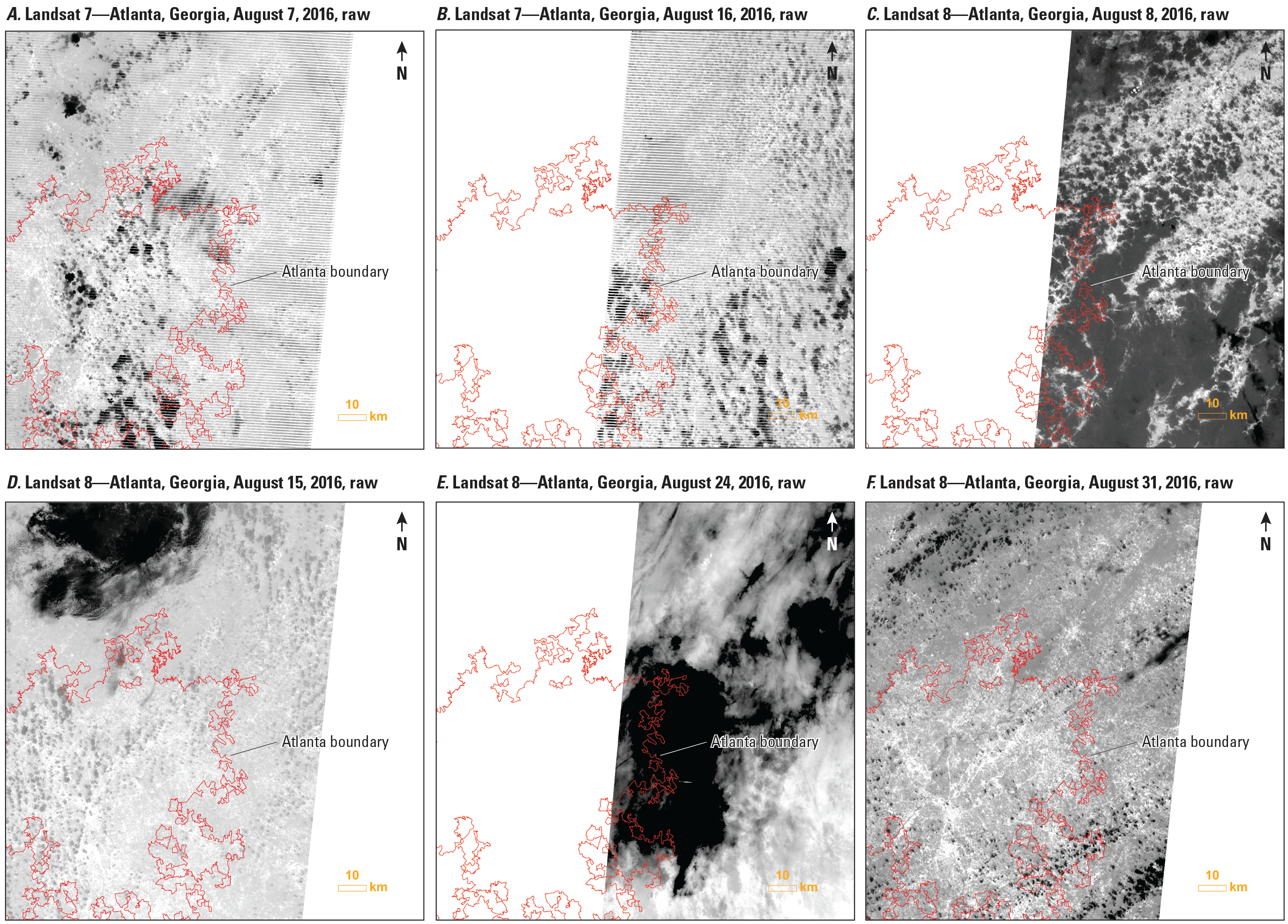
Original Landsat Analysis Ready Data surface temperature records from the tile in the Atlanta, Georgia, area in August 2016. A, Landsat 7 image from August 7, 2016; B, Landsat 7 image from August 16, 2016; C, Landsat 8 image from August 8, 2016; D, Landsat 8 image from August 15, 2016; E, Landsat 8 image from August 24, 2016; F, Landsat 8 image from August 31, 2016.
Seasonal and Annual Variations of Land Surface Temperature Data
LST is highly related to incoming solar radiation and surface physical conditions. The high LST usually coincides with areas of high air temperature because higher LST can lead to higher air temperature through surface heat fluxes (Good and others, 2017; Xian and others, 2022). Air observational networks are, however, sparse and often nonrepresentative in complex anthropogenic landscapes. In the UHI study, for example, temperature differences between urban and rural areas are required; however, not every city has pairs of rural and urban weather stations, and it is difficult to rely on in situ data alone to obtain information about the UHI. Therefore, remotely sensed LST data are increasingly used as a convenient and accessible means to characterize UHIs or surface UHIs. However, the data gaps within Landsat ARD reduce the utility of these data sources to represent close to true seasonal or annual landscape conditions for modeling and monitoring environmental phenomena including surface UHIs. Magnitudes of Landsat ST and MODIS LST of a cloud-free pixel in 2016 from the same weather station site are shown in figure 2. Daily mean temperature data collected by the weather station (National Centers for Environmental Information, 2022) on the same day that Landsat cloud-free ST data were available also are shown in figure 2. Air temperatures that are observed above the ground are relatively larger than remotely sensed LST during cold months when insolation is low and atmospheric fluxes are large. During warm months, remotely sensed LSTs are relatively larger than surface air temperatures. Comparing with MODIS LST and climate observations, Landsat ST records, including Landsat 7 and 8, do not have enough clear records in every month for monthly means estimated from these records to represent the true thermal condition and its variation. The annual mean averaged from monthly means, therefore, will not be close to the true condition.
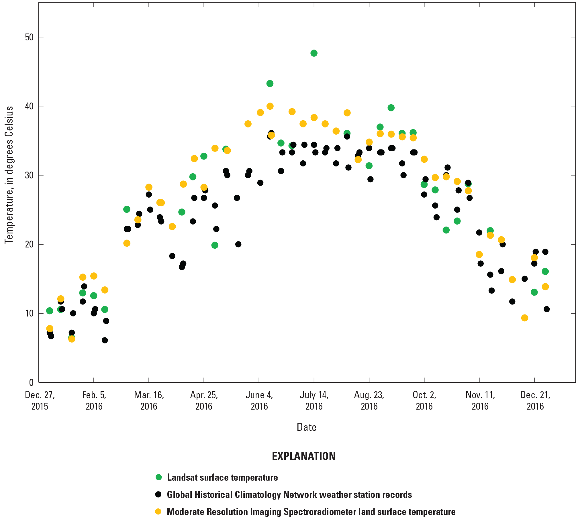
Landsat surface temperature, Global Historical Climatology Network weather station records (National Centers for Environmental Information, 2022), and Moderate Resolution Imaging Spectroradiometer land surface temperature in the Atlanta, Georgia, area in 2016. Landsat and Moderate Resolution Imaging Spectroradiometer data are selected from the same weather station site.
Gap-Filling Approach
The gap-filling method is based on a data-driven spatiotemporal gap-filling approach, which fills the missing pixel value using good pixels from the Worldwide Reference System-2 path overlap region. The satellite orbits are offset to allow 8-day repeat coverage of any Landsat scene area for one Landsat sensor. If more than two Landsat satellites are in operation, the revisit frequency will be larger than a single satellite. The gap-filling approach is based on the assumption that the orbit overlap region of the satellite’s remotely sensed imagery often maintains higher data density than the surrounding nonoverlap area (Zhou and others, 2020). Usually, a Landsat ARD tile contains two to three overlap regions. Many of these data in the overlap region can have similar spectral features with pixels that have the same land cover type within an ARD tile. Pixels in an ARD tile are usually from multiple Landsat paths/rows on different dates. For a given pixel time series in an ARD tile, good quality pixels can be modeled as a linear combination of a set of pixel time series from the orbit overlap region. Therefore, we can model the time-series seasonality for any given pixel using training pixels in the same month or season as the overlap region in the same tile.
Generally, the data gap is defined as absent pixels because of the swath coverage or cloud-contaminated observations determined from the Landsat pixel Quality Assessment band. The gap-filling approach used in this study contains the following steps: (1) training data selection, (2) training data refinement, (3) training sample selection, (4) linear regression model creation, and (5) time-series prediction.
Step 1. Potential training data selection.—This step identifies if data are missing in time-series images in an ARD tile. Pixels in the orbit overlap regions are then identified and extracted using the thresholds based on peak values of histograms of clear observations in overlap and nonoverlap regions.
Step 2. Reprocessing data in overlap regions.—Because time-series images in overlap regions may contain cloud-contaminated pixels, these data need to be processed to exclude these contaminated pixels before they can serve as training samples. A Harmonic Adaptive Penalty Operator (HAPO) algorithm (Zhou and others, 2022) is implemented to replace these contaminated pixels. The HAPO method first uses a seven-parameter linear harmonic model (eq. 1) to replace these pixels.
whereis the predicted value for the ith Landsat band at ordinal date t (because this study is only used for LST gap filling, only one band is used so i is 1),
i
is the ith Landsat band,
c0,i and c1,i
are the estimated intercept and slope coefficients for the ith Landsat band,
t
is the ordinal of the date when January 1 of the year zero has ordinal 1 (sometimes called Julian date),
n
is the frequency of the harmonic model,
an,i and bn,i
are the estimated nth order harmonic coefficients for the ith Landsat band,
ω
is the base annual frequency (2π⁄T), and
T
is the length of the time period (T=365.25).
After fitting, HAPO adjusts parameters in the harmonic regression listed in equation 1 by removing the linear trend (c0+c1t) first. Then, HAPO normalizes the time series to ensure that the algorithm is robust to time series with different magnitudes. Two measures, the sum of squared residuals and a penalty function, are minimized in the calculation of regression model coefficients. The sum of squared residuals, which is defined in equation 2, minimizes the total difference between observations and model predictions. The penalty function, which is defined in equation 3, estimates the variance of the model curve.
whereSSR
is the sum of squared residuals,
N
is the total number of observations in the time series,
i
is the number of observations, and
yi and
are observed and model predicted magnitudes.
P
is a penalty function,
β
is used to adjust the intensity of smooth effect and is set as 1,
n
is the frequency of the harmonic model, and
variables of Ann and An
are calculated in the following equations.
an and bn
are coefficients from equation 1 and
n
is the same as in equation 3.
Step 3. Clustering the training data.—After the potential training pixels are produced in step 2, the training data sources are clustered based on the Euclidean distance to meet time-series similarity so that the training samples can be stratified based on their similarity to the target pixel. The Kmeans analysis method is used to calculate the averages of time series in each cluster center, and the training data are clustered into 20 groups based on these means.
Step 4. Training data selection.—The training data are randomly stratified from multiple clusters so that some mixed pixel time series can have combined seasonality from different landscapes. The Euclidean distances from cluster centers to the target pixel are calculated and the inverse distances are used as the weights to randomly sample a total of 100 pixels from the training data. The stratified sampling strategy emphasizes training data with similar seasonality but is not restricted by clusters; therefore, the approach is robust when the target pixel has a similar distance to multiple cluster centers, which could be the case for mixed pixels.
Step 5. The full time-series prediction.—After training samples are selected, the samples are used to create linear regression models to predict time series of any target pixel. The least absolute shrinkage and selection operator regression (eq. 6) is used to build regression models to predicted values at gaps based on clear observations from the training pixels.
wherey
is the targeted time-series pixel in a clear observation date,
α0 and αi
are linear parameters,
M
is the total of training samples,
Yi
is sampled training data, and
ε
is the error.
The workflow of the gap-filling procedures is shown in figure 3. The steps highlighted in the box with the dashed line are repeated 10 times for each target pixel. The median and standard deviation (STD) values from each time step are produced in the final prediction. The median value is used for gap filling, and the STD value is used as an indicator of uncertainty of the model prediction. Generally, the gap-filling procedures are only applied to these containment pixels and no-data pixels. Each ARD tile has a minimum of four Landsat ST tiles every month if records from only one Landsat sensor are available. In most of these ARD tiles, only a part of a tile has the Landsat ST record, as shown in figure 1. After gap filling, each ARD tile will be filled; therefore, at least four records can be used to calculate monthly means in every month. The maximum magnitude of a pixel in a month is used to represent the maximum Landsat ST for the month. The seasonal mean Landsat ST values are calculated from three monthly means, and seasonal maximum is averaged from the maximum values of 3 months.
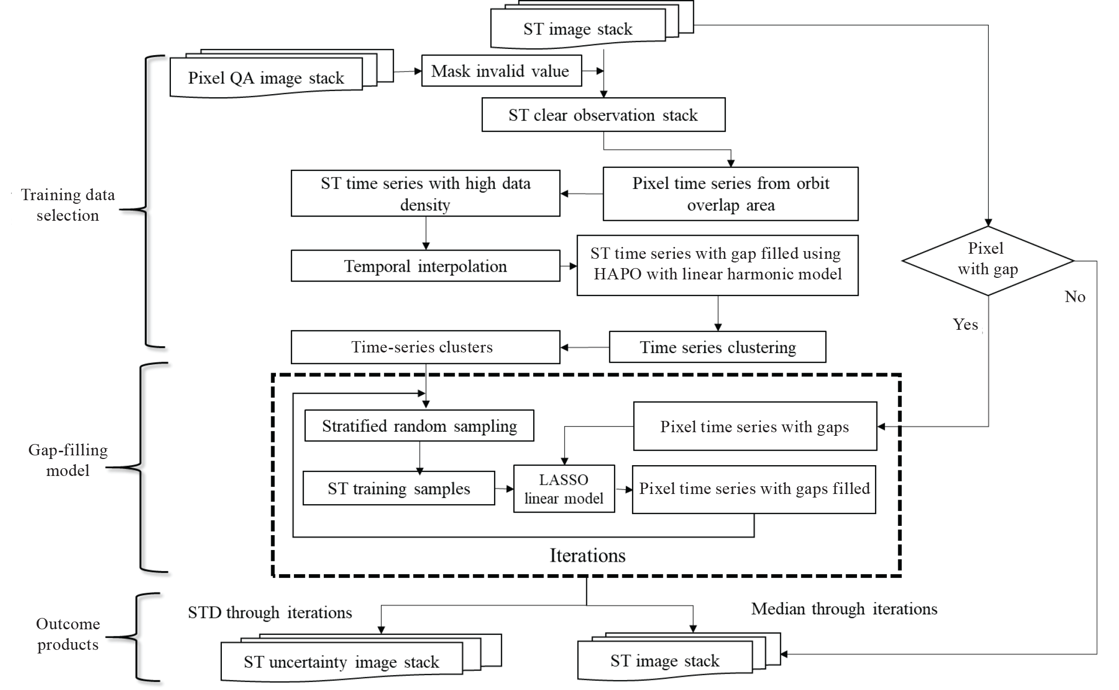
Workflow for the major procedures of the gap-filling algorithm. [QA, Quality Assessment; ST, surface temperature; HAPO, Harmonic Adaptive Penalty Operator; LASSO, least absolute shrinkage and selection operator; STD, standard deviation]
Data Validation
After the gap-filling algorithm is used to produce filled Landsat ST magnitudes in an ARD tile, other ST records are used to evaluate filled Landsat ST data. Here, we use the Atlanta area gap-filling result to illustrate the validation result of filled data. The independent reference datasets for validation are from three major sources: the MODIS LST collection, surface air temperature records observed by the same weather station used in figure 2 (National Centers for Environmental Information, 2022), and gridded climate data from Daymet (Thornton and others, 2021). The MODIS record is used because it collected imagery consistently every 8 days and the data can be used as a reference to compare with the temporal frequency of filling data. Also, climate data are selected in the days that Landsat ST records are available. About 300 sampling pixels are randomly selected in the study tile. The climate records are used to evaluate temporal variation patterns between climate data and Landsat ST data. The comparison between gridded climate data and remotely sensed LST can generate several statistical parameters, including root mean square error (RMSE) and coefficient of determination (r2) between the reference and filled pixel values, to determine the connections between these data.
Results for Gap-Filled Surface Temperature Data
This section of the report describes the gap-filled Landsat ST data and provides a comparison between the gap-filled and raw Landsat ST data. Lastly, a validation is provided of the gap-filled ST data using MODIS and gridded climate data.
Gap-Filled Landsat Surface Temperature Data
The U.S. ARD tile (h24v13, where h denotes horizontal and v denotes vertical) that covers the southeastern side of the Atlanta area was chosen as the study tile. Most of Atlanta is included within the tile. The gap-filled procedures first used all available images in 1 month to produce an image to represent observed Landsat ST for that month. After gap filling, all derived clear pixels from different dates were averaged to generate the monthly Landsat ST imagery. These monthly Landsat ST data were averaged to produce seasonal and annual Landsat ST means to represent observed Landsat ST means in a specific season and year. The seasonal mean in this study is defined as follows: January–March is season 1 (SN1), April–June is season 2 (SN2), July–September is season 3 (SN3), and October–December is season 4 (SN4). The gap-filled Landsat ST in the same month and year as shown in figure 1 and the related uncertainty map are shown in figure 4A and B. The gap-filled algorithm filled every pixel that is either contaminated by cloud/shadow or has no data with extrapolated magnitudes in a tile from regression models. After gap filling, the tile was filled with estimated and original clear pixels from six dates; therefore, the monthly mean was calculated from the Landsat STs of these six dates to represent the monthly status of Landsat ST. The uncertainty map indicates that uncertainties are reduced for most of the urban area pixels. Higher uncertainties are observed in some nonurban pixels in the eastern and northwestern parts of the Atlanta metropolitan area. These areas have relatively large cloud cover or are without records (fig. 1). Most of the data used for gap filling are from the central part of the tile.
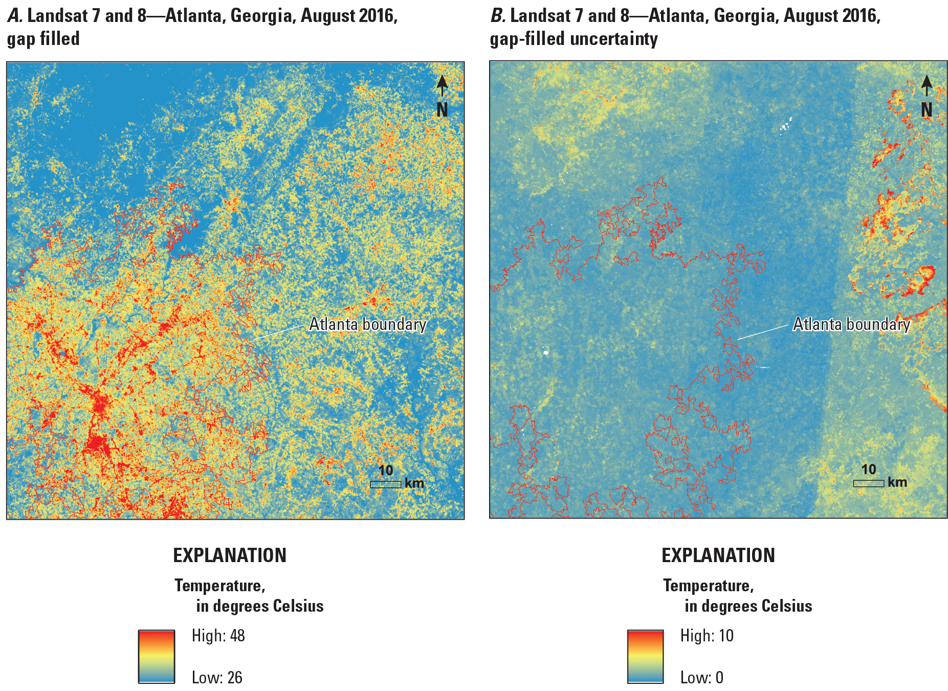
Gap-filled data for Atlanta, Georgia, August 2016. A, gap-filled Landsat surface temperature image; B, uncertainty map.
The monthly means of gap-filled Landsat ST were further averaged to have seasonal means. The Landsat ST seasonal means from gap-filled images were compared with Landsat ST seasonal means estimated directly from available clear pixels without gap filling. Landsat ST seasonal means in 2016 without gap filling are shown in figure 5A–D. The images cover most of the Atlanta urban area. Landsat ST in SN1 shows relatively large magnitudes that are unreasonably high in Landsat ST (fig. 5A). Landsat STs in SN2 and SN4 contain many pixels that are potentially affected by clouds/shadows, resulting in relatively small magnitudes of Landsat ST in most urban areas (fig. 5B, D). The Landsat ST seasonal means indicate urban warming in most urban areas, but they also consist of unreasonably low Landsat STs in some parts of the area. A clear seamline also is observed in SN1, SN2, and SN4. SN3 shows relatively large Landsat ST magnitudes in most urban areas (fig. 5C). The gap-filled Landsat STs fixed unreasonably high seasonal magnitudes in SN1 (fig. 6A) and SN4 (fig. 6D) and low seasonal magnitudes in SN2 (fig. 6B). The gap-filled Landsat ST in SN3 indicates that most pixels in the urban area have larger magnitudes than many surrounding nonurban areas (fig. 6C). The Landsat ST seasonal means do not contain pixels having relatively small magnitudes in the urban area, resulting in clear UHI spatial distribution patterns in all four seasons.
The uncertainty maps of gap-filled pixels in these four seasons are shown in figure 7A–D for SN1–SN4. Generally, the areas that have more data have fewer uncertainties and STD values are relatively small. The strips in the middle of the tile indicate relatively low uncertainties because the area represents the overlap area of multiple Landsat paths/rows. Several areas in the northwestern corner of the tile have relatively high uncertainty pixels. The uncertainties are relatively low in most of the urban areas.
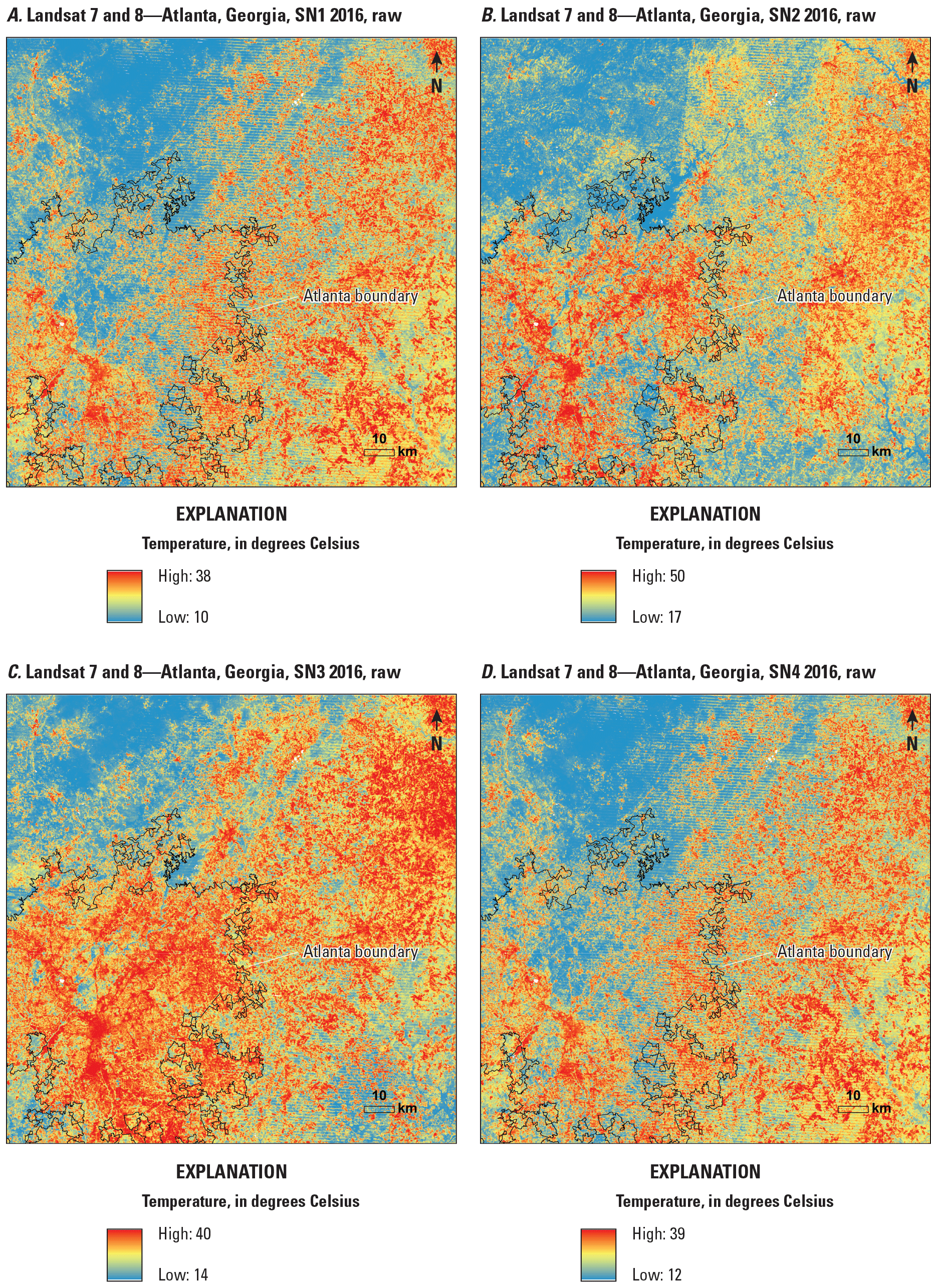
Seasonal Landsat surface temperature means without gap filling in Atlanta, Georgia, 2016. A, season 1 (SN1; January–March); B, season 2 (SN2; April–June); C, season 3 (SN3; July–September); D, season 4 (SN4; October–December).
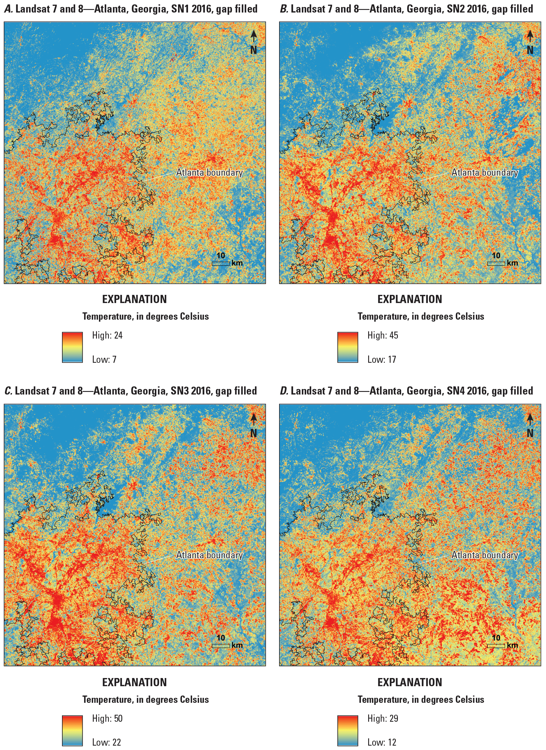
Seasonal Landsat surface temperature with gap filling in Atlanta, Georgia, 2016. A, season 1 (SN1; January–March); B, season 2 (SN2; April–June); C, season 3 (SN3; July–September); D, season 4 (SN4; October–December).
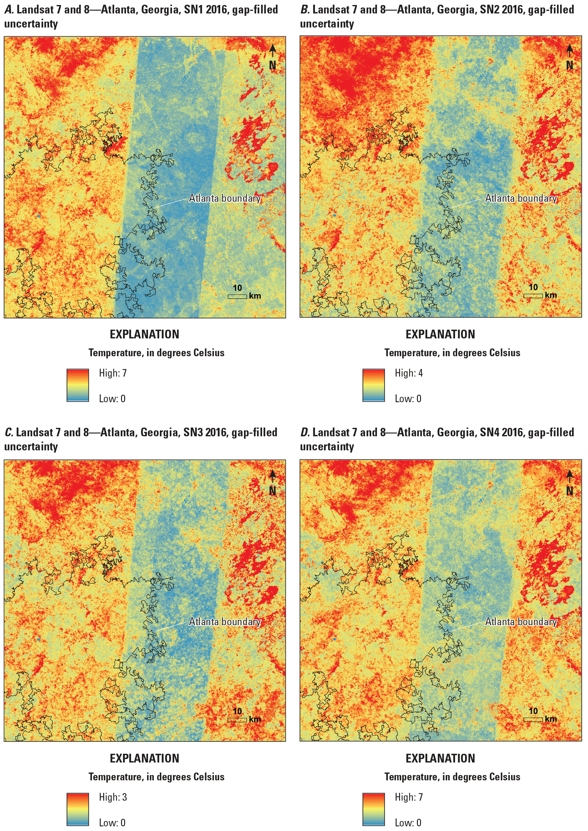
Uncertainty for seasonal Landsat surface temperature with gap filling in Atlanta, Georgia, 2016. A, season 1 (SN1; January–March); B, season 2 (SN2; April–June); C, season 3 (SN3; July–September); D, season 4 (SN4; October–December).
Comparisons of Gap-Filled Data with Raw Landsat Surface Temperature Data
The annual variation of single pixel gap-filled Landsat ST at the same location used in figure 2 was compared with nongap-filled Landsat ST, MODIS LST, and climate records in 2016 (fig. 8). The gap-filled Landsat ST added more records in warm months. These increasing records improved the temporal density of Landsat ST, resulting in better estimates of monthly and seasonal means in these warm seasons. In cold months, the gap-filled Landsat STs are slightly elevated by including more cloud/shadow-free pixels that are warmer than cloud/shadow-contaminated pixels. The gap-filled Landsat STs have a temporal variation pattern that is similar to the pattern from MODIS and weather station records.
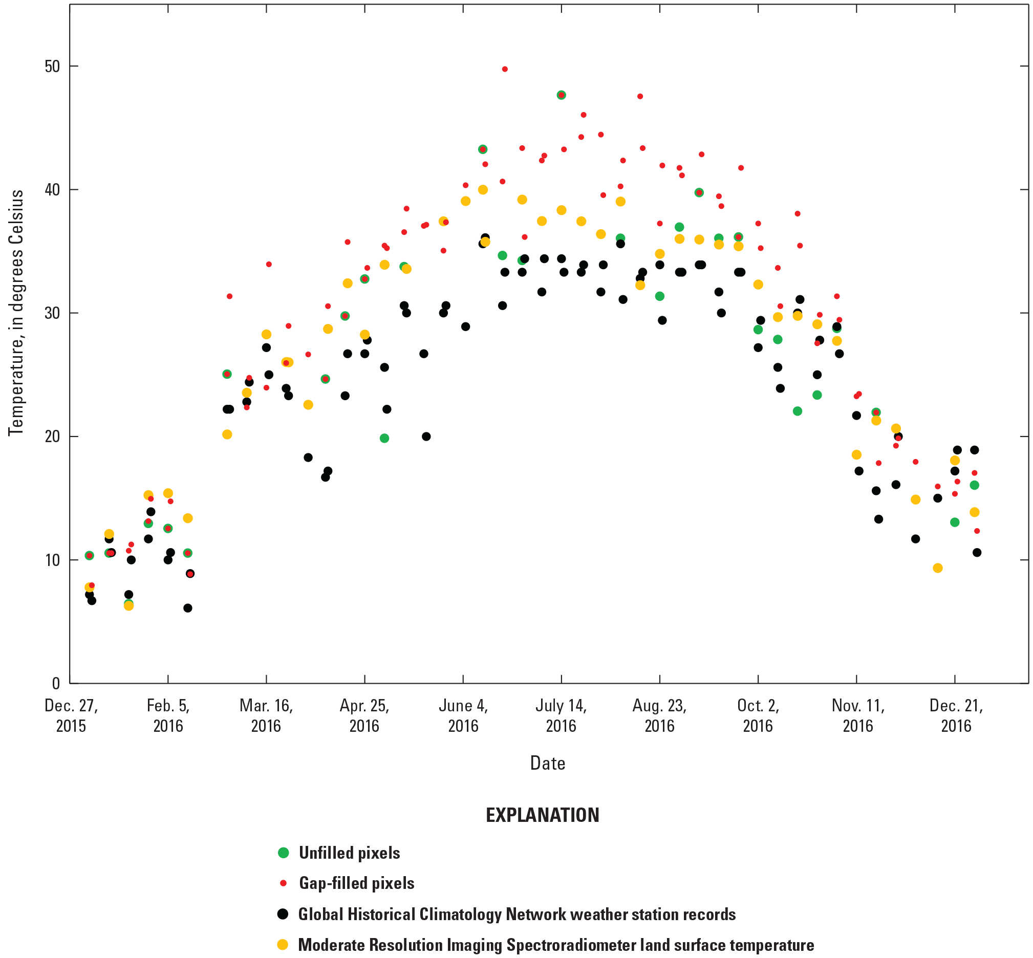
Landsat surface temperatures from original pixels without gap-filling, gap-filled pixels, Global Historical Climatology Network climate records (National Centers for Environmental Information, 2022), and Moderate Resolution Imaging Spectroradiometer land surface temperature in 2016.
Validation of Gap-Filled Landsat Surface Temperature Data Using Moderate Resolution Imaging Spectroradiometer Land Surface Temperature and Gridded Climate Data
We used randomly stratified samples over urban and agricultural lands to compare gap-filled Landsat ST and Daymet daily maximum air temperature (number of samples [n] =86), gap-filled Landsat ST and MODIS LST (n=44), and MODIS LST and Daymet maximum air temperature records (n=44). Statistically correlated outcomes including correlation of determination (r2), standard error (SE), and RMSE are provided in table 1. The gap-filling Landsat ST samples over urban land have relatively higher correlations and lower SE and RMSE values than Daymet records and MODIS data over agricultural land. However, MODIS LSTs have similar correlations and SEs with air temperature but higher RMSE values in the urban area. Scatter plots of gap-filling Landsat ST versus air temperature (fig. 9A) and gap-filling Landsat ST versus MODIS LST (fig. 9B) in 2016 from randomly selected samples are shown in figure 9. The gap-filling Landsat ST and air temperature are highly correlated and have an r2 value of 0.88, but Landsat ST values are greater than air temperature. The MODIS LST also has a relatively high and significant correlation at a less than 1-percent level (probability [or P] less than 0.01) with Landsat ST and has an r2 value of 0.92.
Table 1.
Correlations of gap-filled Landsat surface temperature, surface air temperature from Daymet gridded climate data, and Moderate Resolution Imaging Spectroradiometer land surface temperature from randomly selected samples in 2016. These samples were collected from urban and agricultural lands. All correlations are statistically significant at a less than 1-percent level (probability [or P] less than 0.01).[MODIS, Moderate Resolution Imaging Spectroradiometer; r2, coefficient of determination; SE, standard error; RMSE, root mean square error]
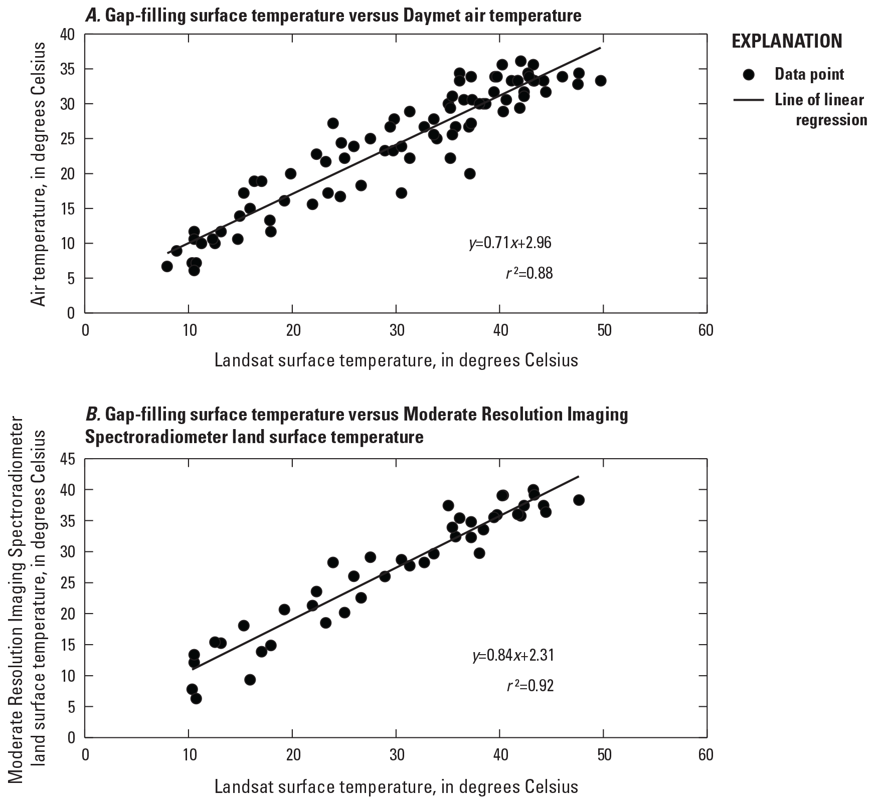
Gap-filled Landsat surface temperature in 2016. A, versus Daymet air temperature; B, versus Moderate Resolution Imaging Spectroradiometer land surface temperature. [r2, coefficient of determination; y, y-axis temperature in Celsius; x, x-axis temperature in Celsius]
Summary and Conclusions
Landsat surface temperature (ST) observations within an Analysis Ready Data tile without gap filling cannot provide sufficient data to represent temporal frequency of surface thermal conditions in a time series, resulting in either overestimates or underestimates of their temporal means. The lack of temporal density information could make the Landsat ST data unreliable in the time-series seasonal or annual change analysis. Filling data gaps to increase data availability is essential for surface thermal condition change analysis using time-series data. This study presents an effective method to fill gaps for the Landsat U.S. Analysis Ready Data ST products.
We used clustering analysis to find orbit overlap region pixels with similar time series to the given pixel for training data selection. More importantly, we iteratively predicted values using multiple randomly selected pixels, which reduced the potential effects of noise in training data and allowed the use of a regression model to estimate the uncertainty of model predictions. After that, we implemented least absolute shrinkage and selection operator regression to estimate the Landsat ST magnitudes for these cloud/shadow-contaminated pixels. The model uncertainty indicated the stability of model predictions instead of the prediction error.
The Landsat ST with gap filling substantially added temporal density for monthly Landsat ST records. The gap-filled Landsat ST has significant correlations with air temperature recorded from gridded weather records, indicating similar monthly variation patterns between the two datasets. Also, the gap-filled Landsat ST data are highly correlated with Moderate Resolution Imaging Spectroradiometer land surface temperature data, which have more frequent temporal coverage but coarse spatial resolution. The uncertainty maps show spatial distributions of uncertainty for gap-filled pixels that have high or low uncertainties. Using gap-filled Landsat ST data allows multidecade time-series Landsat ST change analysis to be completed consistently. The gap-filled images in this study used the Landsat Quality Assessment band to identify clouds and shadows. The biases from the Quality Assessment band can affect the quality of training samples and the gap-filled image. Improved Quality Assessment information that can better identify clouds and shadows can improve the gap-filling approach when it is implemented to process large areas of Landsat ST data in an automatic manner.
References Cited
Buchhorn, M., Lesiv, M., Tsendbazar, N.-E., Herold, M., Bertels, L., and Smets, B., 2020, Copernicus Global Land Cover layers—Collection 2: Remote Sensing, v. 12, no. 6, art. 1044, 14 p. [Also available at https://doi.org/10.3390/rs12061044.]
Chen, Y., Cao, R., Chen, J., Liu, L., and Matsushita, B., 2021, A practical approach to reconstruct high-quality Landsat NDVI time-series data by gap filling and the Savitzky–Golay filter: ISPRS Journal of Photogrammetry and Remote Sensing, v. 180, p. 174–190. [Also available at https://doi.org/10.1016/j.isprsjprs.2021.08.015.]
Cook, M., Schott, J., Mandel, J., and Raqueno, N., 2014, Development of an operational calibration methodology for the Landsat thermal data archive and initial testing of the atmospheric compensation component of a land surface temperature (LST) product from the archive: Remote Sensing (Basel), v. 6, no. 11, p. 11244–11266. [Also available at https://doi.org/10.3390/rs61111244.]
Deilami, K., Kamruzzaman, M., and Liu, Y., 2018, Urban heat island effect—A systematic review of spatio-temporal factors, data, methods, and mitigation measures: International Journal of Applied Earth Observation and Geoinformation, v. 67, p. 30–42. [Also available at https://doi.org/10.1016/j.jag.2017.12.009.]
Gao, F., Hilker, T., Zhu, X., Anderson, M., Masek, J., Wang, P., and Yang, Y., 2015, Fusing Landsat and MODIS data for vegetation monitoring: IEEE Geoscience and Remote Sensing Magazine, v. 3, no. 3, p. 47–60. [Also available at https://doi.org/10.1109/MGRS.2015.2434351.]
Good, E.J., Ghent, D.J., Bulgin, C.E., and Remedios, J.J., 2017, A spatiotemporal analysis of the relationship between near-surface air temperature and satellite land surface temperatures using 17 years of data from the ATSR series: Journal of Geophysical Research Atmospheres, v. 122, no. 17, p. 9185–9210. [Also available at https://doi.org/10.1002/2017JD026880.]
Malakar, N.K., Hulley, G.C., Hook, S.J., Laraby, K., Cook, M., and Schott, J.R., 2018, An operational land surface temperature product for Landsat thermal data—Methodology and validation: IEEE Transactions on Geoscience and Remote Sensing, v. 56, no. 10, p. 5717–5735. [Also available at https://doi.org/10.1109/TGRS.2018.2824828.]
National Centers for Environmental Information, 2022, Global Historical Climatology Network daily (GHCNd): National Centers for Environmental Information digital data, accessed May 17, 2022, at https://www.ncei.noaa.gov/products/land-based-station/global-historical-climatology-network-daily.
Pincebourde, S., and Salle, A., 2020, On the importance of getting fine-scale temperature records near any surface: Global Change Biology, v. 26, no. 11, p. 6025–6027. [Also available at https://doi.org/10.1111/gcb.15210.]
Stewart, I.D., Krayenhoff, E.S., Voogt, J.A., Lachapelle, J.A., Allen, M.A., and Broadbent, A.M., 2021, Time evolution of the surface urban heat island: Earth’s Future, v. 9, no. 10, art. e2021EF002178, 9 p. [Also available at https://doi.org/10.1029/2021EF002178.]
Thornton, P.E., Shrestha, R., Thornton, M., Kao, S.-C., Wei, Y., and Wilson, B.E., 2021, Gridded daily weather data for North America with comprehensive uncertainty quantification: Scientific Data, v. 8, no. 1, art. 190, 17 p. [Also available at https://doi.org/10.1038/s41597-021-00973-0.]
Tran, D.T., Pla, F., Latorre-Carmona, P., Myint, S.W., Caetano, M., and Kieu, H.V., 2017, Characterizing the relationship between land use and land cover change and land surface temperature: ISPRS Journal of Photogrammetry and Remote Sensing, v. 124, p. 119–132. [Also available at https://doi.org/10.1016/j.isprsjprs.2017.01.001.]
Trlica, A., Hutyra, L.R., Schaaf, C.L., Erb, A., and Wang, J.A., 2017, Albedo, land cover, and daytime surface temperature variation across an urbanized landscape: Earth’s Future, v. 5, no. 11, p. 1084–1101. [Also available at https://doi.org/10.1002/2017EF000569.]
Venter, Z.S., Brousse, O., Esau, I., and Meier, F., 2020, Hyperlocal mapping of urban air temperature using remote sensing crowdsourced weather data: Remote Sensing of Environment, v. 242, art. 111791, 14 p. [Also available at https://doi.org/10.1016/j.rse.2020.111791.]
Voogt, J.A., and Oke, T.R., 2003, Thermal remote sensing of urban climates: Remote Sensing of Environment, v. 86, no. 3, p. 370–384. [Also available at https://doi.org/10.1016/S0034-4257(03)00079-8.]
Weiss, D.J., Atkinson, P.M., Bhatt, S., Mappin, B., Hay, S.I., and Gething, P.W., 2014, An effective approach for gap-filling continental scale remotely sensed time-series: ISPRS Journal of Photogrammetry and Remote Sensing, v. 98, p. 106–118. [Also available at https://doi.org/10.1016/j.isprsjprs.2014.10.001.]
Xian, G., Shi, H., Auch, R., Gallo, K., Zhou, Q., Wu, Z., and Kolian, M., 2021, The effects of urban land cover dynamics on urban heat island intensity and temporal trends: GIScience & Remote Sensing, v. 58, no. 4, p. 501–515. [Also available at https://doi.org/10.1080/15481603.2021.1903282.]
Xian, G., Shi, H., Zhou, Q., Auch, R., Gallo, K., Wu, Z., and Kolian, M., 2022, Monitoring and characterizing multi-decadal variations of urban thermal condition using time-series thermal remote sensing and dynamic land cover data: Remote Sensing of Environment, v. 269, art. 112803, 16 p. [Also available at https://doi.org/10.1016/j.rse.2021.112803.]
Yan, L., and Roy, D.P., 2020, Spatially and temporally complete Landsat reflectance time series modelling—The fill-and-fit approach: Remote Sensing of Environment, v. 241, art. 111718, 17 p. [Also available at https://doi.org/10.1016/j.rse.2020.111718.]
Zhang, X., Liu, L., Chen, X., Gao, Y., Xie, S., and Mi, J., 2021, GLC_FCS30—Global land-cover product with fine classification system at 30 m using time-series Landsat imagery: Earth System Science Data, v. 13, no. 6, p. 2753–2776. [Also available at https://doi.org/10.5194/essd-13-2753-2021.]
Zhou, Q., Xian, G., and Shi, H., 2020, Gap fill of land surface temperature and reflectance products in Landsat analysis ready data: Remote Sensing (Basel), v. 12, no. 7, art. 1192, 16 p. [Also available at https://doi.org/10.3390/rs12071192.]
Zhou, Q., Zhu, Z., Xian, G., and Li, C., 2022, A novel regression method for harmonic analysis of time series: ISPRS Journal of Photogrammetry and Remote Sensing, v.185, p. 48–61. [Also available at https://doi.org/10.1016/j.isprsjprs.2022.01.006.]
Zhu, X., Liu, D., and Chen, J., 2012, A new geostatistical approach for filling gaps in Landsat ETM+ SLC-off images: Remote Sensing of Environment, v. 124, p. 49–60. [Also available at https://doi.org/10.1016/j.rse.2012.04.019.]
Abbreviations
ARD
Analysis Ready Data
HAPO
Harmonic Adaptive Penalty Operator
LST
land surface temperature
MODIS
Moderate Resolution Imaging Spectroradiometer
n
number of samples
NDVI
Normalized Difference Vegetation Index
r2
coefficient of determination
RMSE
root mean square error
SN1
season 1 (January–March)
SN2
season 2 (April–June)
SN3
season 3 (July–September)
SN4
season 4 (October–December)
ST
surface temperature
STD
standard deviation
UHI
urban heat island
For more information about this publication, contact:
Director, USGS Earth Resources Observation and Science Center
47914 252nd Street
Sioux Falls, SD 57198
605–594–6151
For additional information, visit: https://www.usgs.gov/centers/eros
Publishing support provided by the
Rolla Publishing Service Center
Suggested Citation
Xian, G., Shi, H., Arab, S., Mueller, C., Hussain, R., Sayler, K., and Howard, D., 2023, Improving temporal frequency of Landsat surface temperature products using the gap-filling algorithm: U.S. Geological Survey Open-File Report 2023–1006, 15 p., https://doi.org/10.3133/ofr20231006.
ISSN: 2331-1258 (online)
Study Area
| Publication type | Report |
|---|---|
| Publication Subtype | USGS Numbered Series |
| Title | Improving temporal frequency of Landsat surface temperature products using the gap-filling algorithm |
| Series title | Open-File Report |
| Series number | 2023-1006 |
| DOI | 10.3133/ofr20231006 |
| Year Published | 2023 |
| Language | English |
| Publisher | U.S. Geological Survey |
| Publisher location | Reston, VA |
| Contributing office(s) | Earth Resources Observation and Science (EROS) Center |
| Description | vi, 15 p. |
| Country | United States |
| State | Georgia |
| City | Atlanta |
| Online Only (Y/N) | Y |
| Google Analytic Metrics | Metrics page |