

Delineating the Pierre Shale from Geophysical Surveys Within and Near Ellsworth Air Force Base, South Dakota, 2019
Links
- Document: Pamphlet (2.44 MB pdf) , HTML , XML
- Sheets:
- Sheet 1 (8.39 MB pdf) — Electrical resistivity tomography inversion results with depth to Pierre Shale from horizontal-to-vertical spectral ratio results for transects 1C1, 1C2, 14, 15, 13A, 13B, 1A, 1B, 4B, and 4C, Ellsworth Air Force Base, South Dakota
- Sheet 2 (10.8 MB pdf) — Electrical resistivity tomography inversion results with depth to Pierre Shale from horizontal-to-vertical spectral ratio results for transects 4A1, 4A2, 2, 3A, 3B, 3C, and 5, Ellsworth Air Force Base, South Dakota
- Sheet 3 (9.47 MB pdf) — Electrical resistivity tomography inversion results with depth to Pierre Shale from horizontal-to-vertical spectral ratio results for transects 9A, 9B, 9C, 11, 8A, 8B, 8C, 10, and 12, Ellsworth Air Force Base, South Dakota
- Dataset: U.S. Geological Survey National Water Information System database — USGS water data for the Nation
- Data Release: USGS data release — Electrical Resistivity Tomography (ERT) and Horizontal-to-Vertical Spectral Ratio (HVSR) data collected within and near Ellsworth Air Force Base, South Dakota, from 2014 to 2019
- Download citation as: RIS | Dublin Core
Acknowledgments
The authors would like to thank the U.S. Air Force Civil Engineering Center for funding assistance and Ellsworth Air Force Base for providing access to field sites.
The authors would also like to thank the U.S. Geological Survey reviewers for their careful reviews and comments.
Abstract
The U.S. Geological Survey, in cooperation with the U.S. Air Force Civil Engineering Center, investigated the use of surface geophysical methods to delineate the top of the Cretaceous Pierre Shale along survey transects in selected areas within and near Ellsworth Air Force Base, South Dakota. Two complementary geophysical methods—electrical resistivity and passive seismic—were used along 26 co-located transect surveys within and near Ellsworth Air Force Base for a total of 12.7 line-kilometers. Electrical resistivity results were analyzed using EarthImager2D electrical resistivity tomography processing and inversion software. Two-dimensional earth models showing the electrical properties of the subsurface were evaluated by directly comparing the high and low subsurface resistivity values to a surficial geologic map and nearby wells with driller logs. Passive seismic data were analyzed using the horizontal-to-vertical spectral ratio method to determine the depth to the Pierre Shale at each survey point. The electrical resistivity and passive seismic results were compared to driller logs from nearby wells to delineate the top of the Pierre Shale. The depth to the Pierre Shale along the transects ranged from about 2.4 to 20.3 meters, and mean and median depths were about 9.2 and 9.0 meters, respectively. The elevation of the Pierre Shale and thickness of unconsolidated deposits generally increased with land-surface elevation from south to north; however, some transects displayed topographically high and low areas that sometimes did not correlate with land-surface topography and may affect local groundwater flow.
Introduction
Ellsworth Air Force Base (EAFB) is next to the town of Box Elder, South Dakota, and is about 10 kilometers northeast of Rapid City, S. Dak. (fig. 1). The current (2021) size of EAFB is about 20 square kilometers and spans Meade and Pennington Counties (U.S. Environmental Protection Agency, 2021). Operations at EAFB began in 1942, and in 1990, EAFB was listed on the U.S. Environmental Protection Agency’s National Priorities List because of contamination in nearby water wells related to military operations. Many investigative and restoration projects have since worked to understand the degree and extent of contamination near EAFB (U.S. Environmental Protection Agency, 2021), as well as treat contaminated areas that have since been removed from the National Priorities List (U.S. Environmental Protection Agency, 2021). Recent investigations have focused on the potential presence of perfluorooctane sulfonate and perfluorooctanoic acid in soil, groundwater, surface water, sediment, and drinking water within and near EAFB (U.S. Environmental Protection Agency, 2021).
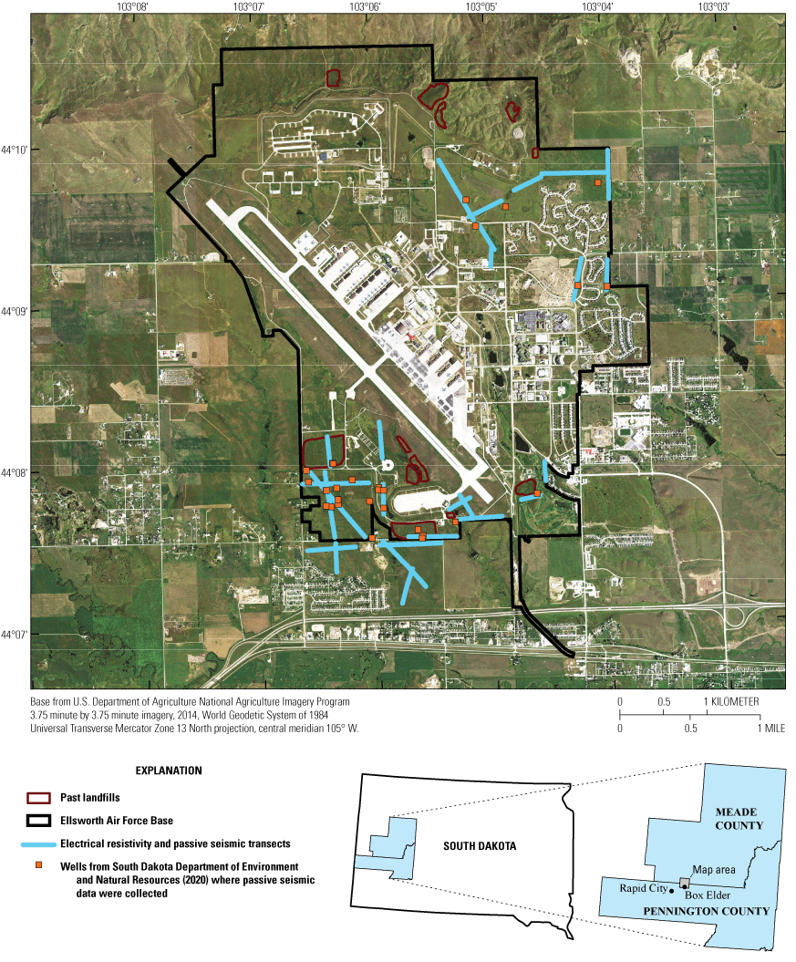
Electrical resistivity and passive seismic transects, past landfills, and wells where passive seismic data were collected within and near Ellsworth Air Force Base, South Dakota.
The U.S. Geological Survey (USGS), in cooperation with the U.S. Air Force Civil Engineering Center, investigated the use of surface geophysical methods to delineate the top of bedrock along survey transects in selected areas within and near EAFB. Geophysical surveys provide a noninvasive means of characterizing hydrogeologic conditions to supplement preexisting information. Two complementary geophysical methods—electrical resistivity and passive seismic—were used along 26 co-located transect surveys within and near EAFB for a total of 12.7 line-kilometers (fig. 1). Electrical resistivity and passive seismic surveys were co-located for direct comparison and to improve interpretation of the bedrock surface. Electrical resistivity data were collected along lines to produce a two-dimensional (2D) image of subsurface resistivity, whereas passive seismic data were collected as soundings to provide a depth to bedrock at a single point.
Purpose and Scope
The purpose of this report is to document the results of two complementary geophysical surveys by the USGS from July to October 2019 within and near EAFB to delineate the top of the Cretaceous Pierre Shale (bedrock). Electrical resistivity and passive seismic surveys were completed along 26 co-located transects for a total of 12.7 line-kilometers. The electrical resistivity and passive seismic surveys were co-located for direct comparison and to complement the delineation of the Pierre Shale along profiles in selected areas. The purpose of delineating the Pierre Shale was to improve the understanding of groundwater flow in unconsolidated deposits overlying the Pierre Shale within and near EAFB.
Geology and Hydrogeology of the Alluvial Aquifer and Pierre Shale
The geology of EAFB was determined using a geologic map (Redden and DeWitt, 2009) and driller logs (South Dakota Department of Environment and Natural Resources, 2020). The geologic map from Redden and DeWitt (2009) showed the study area consists of Cretaceous Pierre Shale, Quaternary terrace deposits, and Quaternary alluvial deposits (fig. 2). The study area also has artificial fill and landfill deposits from historical and recent activities on EAFB (not shown in fig. 2). Driller logs in the study area (South Dakota Department of Environment and Natural Resources, 2020) have recovered landfill waste (clothing scraps, glass, and wood) at several locations from various depths in areas of past landfills (fig. 1).
The youngest geologic unit at EAFB is the unconsolidated Quaternary alluvial deposits that are near active streams and consist of mud, silt, sand, and gravel with a maximum thickness of about 10 meters (m) (fig. 2; Redden and DeWitt, 2009). Unconsolidated Quaternary terrace deposits underlie most of the EAFB and are generally older and at greater elevation than alluvial deposits in the study area. The terrace deposits in the study area formed from remnants of past river systems that incised into the landscape and left behind deposits of gravel, sand, silt, and soils (McGregor and Cattermole, 1973; Redden and DeWitt, 2009). The terrace deposits can be as much as 30 m thick in the study area (Redden and DeWitt, 2009), although driller logs indicated a mean thickness of 10 m (South Dakota Department of Environment and Natural Resources, 2020). The Pierre Shale is the bedrock unit in the study area and is exposed at the surface in some areas (fig. 2). The Pierre Shale unconformably underlies Quaternary alluvial deposits and Quaternary terrace deposits with an erosional contact (Redden and DeWitt, 2009). Driller logs from the South Dakota Department of Environment and Natural Resources (2020) in the study area show that the upper 4.5 to 10.0 m of the Pierre Shale can be highly weathered and fractured with oxidized iron staining.
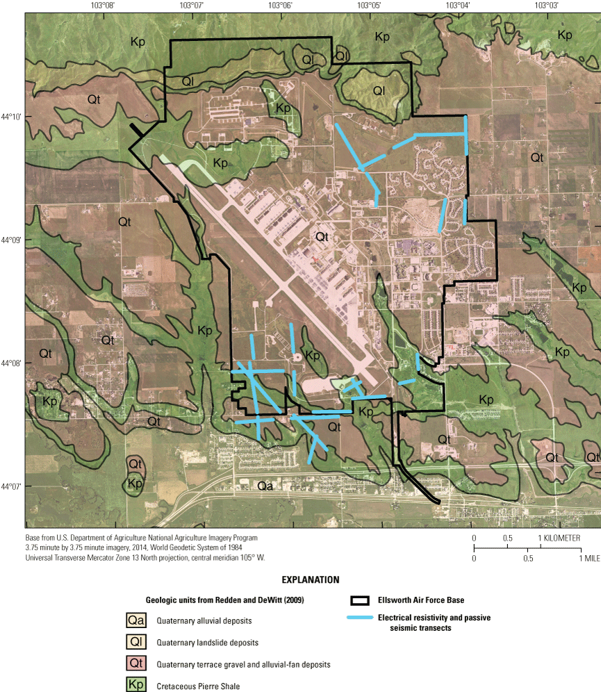
Surficial geology and electrical resistivity and passive seismic transects within and near Ellsworth Air Force Base, South Dakota.
The hydrogeology of the study area was interpreted from lithologic descriptions in driller logs (South Dakota Department of Environment and Natural Resources, 2020). Driller logs indicated coarse, unconsolidated materials in Quaternary alluvial and terrace deposits overlying the Pierre Shale contain groundwater and compose the shallow unconfined aquifer at EAFB. The shallow unconfined aquifer is recharged by direct infiltration of precipitation at the land surface. Coarse materials in the shallow unconfined aquifer, such as sand and gravel, facilitate groundwater flow because of the larger pore spaces and greater hydraulic conductivity. Finer materials, such as clay and silt, act as barriers to groundwater flow but can store substantial amounts of water in pore spaces. Similarly, driller logs have shown that the upper weathered surface of the Pierre Shale contains water; however, groundwater flow in the Pierre Shale likely is minimal because of its low hydraulic conductivity (Bredehoeft and others, 1983). The direction of groundwater flow in the shallow unconfined aquifer approximates surface topography in the absence of structures, such as buried stream channels (Heath, 1983).
Geophysical Surveying Methods
The geophysical methods used to estimate the thickness of unconsolidated Quaternary deposits and the geometry of the Pierre Shale at EAFB were electrical resistivity tomography (ERT) and a passive seismic technique called the horizontal-to-vertical spectral ratio (HVSR) method. In total, the USGS surveyed 26 transects for a total of 12.7 line-kilometers between July and October 2019 within and near EAFB (fig. 1). The ERT and HVSR surveys were co-located along predetermined transects in selected areas to determine the depth to the Pierre Shale and to allow for comparison between results of both methods. Latitude, longitude, and land-surface elevation data were collected at electrical-resistivity survey electrodes using real-time kinematic (RTK) surveys. Global Positioning System locations and elevations from light detection and ranging survey data were used to accurately locate HVSR sites. All geophysical data and site information (latitude, longitude, and elevation) are available as a USGS data release (Medler and others, 2021).
Electrical Resistivity
2D electrical resistivity surveys were completed at EAFB to characterize subsurface materials and determine the depth to bedrock along profiles. Electrical resistivity surveys identify horizontal and (or) vertical changes in subsurface resistivity that typically correspond to changes in lithology, chemistry of pore fluids, and (or) water content of subsurface materials (Sheets, 2002). 2D electrical resistivity surveys are commonly done using many electrodes equally spaced along a straight transect. The spacing of electrodes along a transect generally controls the depth of investigation and the measurement resolution. Greater electrode spacing corresponds to greater a depth of investigation but lower measurement resolution, whereas finer electrode spacing corresponds to a smaller depth of investigation but higher measurement resolution (Loke, 1999). The electrodes are connected to stainless steel takeouts spaced at a regular interval along a cable, which is connected to the resistivity meter that controls the measurements. The resistivity meter runs a pre-programmed data-collection routine that automatically selects (at least) four electrodes for each measurement. Measurements consist of two current electrodes and (at least) two potential electrodes; electrical current is transmitted into the ground through current electrodes, and the resulting voltage is measured at the potential electrodes. Electrode groupings and the sequence of measurements are controlled by the type of array specified for the survey. Commonly used arrays include Wenner, dipole-dipole, and Schlumberger (Loke, 1999, 2004). Electrical resistivity data are then downloaded from the resistivity meter after the survey is complete and modeled using tomographic inversion software to obtain 2D cross sections of the subsurface resistivity.
Electrical resistivity data were acquired at EAFB between June and October 2019 using an 8-channel, SuperSting R8 resistivity meter (Advanced Geosciences Inc., 2020) with 56 total electrodes on 4 cable sections (14 electrodes per cable section). Electrodes along each cable were connected to stainless steel stakes placed at evenly spaced intervals (3 to 5 m) along predetermined transects on the land surface. The land surface was sprayed with freshwater after placing electrodes to reduce electrical contact resistance with the ground before data collection. Cables two and three were then connected to the SuperSting R8 that automatically collected resistivity data by switching between programmed combinations of current and potential electrode pairs based on the dipole-dipole array configuration. Loke (1999) and Zohdy and others (1974) provide a description of the dipole-dipole array.
Some of the longer transects required the “roll-along” technique to extend the horizontal area covered by the survey. The “roll-along” technique involved moving the first electrode cable section (electrodes 1 to 14) at the front of the survey to the end of initially placed cables with 75-percent overlap of the previous cable layout until the desired length of transect was completed. Data-collection errors, which were caused by electrodes not properly transmitting and receiving electrical signals, were noticed in transects that required the “roll-along” technique. The data-collection errors resulted in data gaps along transects and required the data to be subset into smaller sections that were processed individually. The sectioned datasets show the electrical resistivity results as if they were collected as “end-to-end” surveys. The “end-to-end” surveys extend the length of the transect by repositioning all electrode cable sections to the end of the initially placed cables. In total, data-collection errors were noticed in 23 of the 26 transects, and transects lengths ranged from 220 to 960 m.
2D ERT models were constructed for each transect using the EarthImager2D tomographic inversion software suite (https://www.agiusa.com/agi-earthimager-2d). The first step in model construction was removal of noisy data automatically and manually in EarthImager2D. The automatic data removal used seven criteria specified by EarthImager2D in the recommended settings. Additionally, noisy data were removed manually before and after inversion using a EarthImager2D utility that allows users to select individual data points that display a data misfit percentage. The second step was to incorporate elevation information using land-surface elevation data from RTK surveys for each electrode to minimize errors from topographic changes.
The third step was to choose the method of inversion and remove noisy data highlighted after inversion. The electrical resistivity data were modeled using least-squares smooth model inversion (Constable and others, 1987; Farquharson and Oldenburg, 1998) because the area surveyed was best approximated as a simple layered model with only two or three layers. Smooth model inversion reduces differences between measured data and predicted values in a simple starting model using an iterative process, where successive iterations attempt to reduce the difference between measured data and predicted values by determining the root mean square (rms) error. The goal of smooth model inversion is to reduce the rms error until a desired error tolerance is met rather than minimize the rms error—which increases model roughness, causes artifacts, and diverges from the simple layered model (Constable and others, 1987). The maximum number of model iterations was set to eight for all ERT transects, and the accepted model was chosen as the model that best fit the site conceptual model and was closest to the convergence criteria. In some instances, data were removed manually after the first inversion to help reduce the rms error and a new inversion was completed. For all ERT transects the model was chosen within the first three iterations, and rms errors were less than 6 percent.
Passive Seismic
Passive seismic data were collected and evaluated using the HVSR method. The HVSR method uses passive seismic data from a single, broad-band, three-component seismometer (Nakamura, 1989; Lane and others, 2007). Passive seismic methods rely on ambient seismic noise generated by wind, ocean waves, and human activities rather than artificial, “active” sources, such as an explosive charge or a hammer blow, to obtain a seismic response (Lane and others, 2008). The HVSR method analyzes ambient seismic noise by using the ratio of two averaged horizontal components (north-south and east-west) to the vertical component (up-down). For each measurement, multiple ratios are averaged to create a single curve from which the fundamental resonance frequency (f0) is determined. The f0 generally is identified as a peak on the curve with the lowest frequency and greatest amplitude.
The f0 can be used to estimate the depth to bedrock through linear regression or if the shear wave velocity (vs) is known or estimated. The linear regression technique involves collecting HVSR data at sites where the depth to bedrock is known and varies, such as a well with information on depth to bedrock. The depth to bedrock (Z) and the f0 are plotted and regressed using equation 1:
where After determining a and b, equation 1 can be applied to calculate depth to bedrock at sites where HVSR data were collected and the f0 was determined but the depth to bedrock is unknown. The other technique involves estimating vs by determining f0 at a site where the depth to bedrock is known using equation 2: If the vs is estimated at many sites where the depth to bedrock is known, a mean vs can be calculated and used to determine the depth to bedrock using equation 3: It is important to note the HVSR method requires a strong acoustic impedance contrast (greater than or equal to 2) between the bedrock and overlying sediments (Lane and others, 2008). The f0 at a site can be difficult to determine without a sufficient contrast.A total of 443 HVSR sites were used to supplement and confirm ERT results in determining the depth to bedrock. A TROMINO Blu three-component seismometer (https://moho.world/en/tromino/) was used to acquire passive seismic data along 26 surveys transects in the study area (fig. 1). Passive seismic measurements were collected every 10–35 m along the transects. At each HVSR site, the seismometer was oriented to north, leveled, and coupled directly to the ground using long spikes to ensure the seismometer was in contact with the land surface. A weighted and inverted 5-gallon bucket was used to protect the seismometer from wind gusts during measurements. One 20-minute measurement was made at each site based on the estimated depth to bedrock being less than 16 m from driller logs (South Dakota Department of Environment and Natural Resources, 2020). Repeat measurements were made at 29 predetermined sites near wells across EAFB where the depth to bedrock was known from driller logs (South Dakota Department of Environment and Natural Resources, 2020; fig. 1). Thirteen of the sites produced clear f0 peaks, which were regressed against the known depth to bedrock to establish a local regression equation. The local regression equation was used to calculate the depth to bedrock at other HVSR sites where the depth to bedrock was unknown along geophysical transects.
The HVSR data were analyzed using the Grilla software suite (https://moho.world/en/tromino/). The Grilla software suite automatically transforms the data from the time domain to the frequency domain using a Fourier Transform and calculates the ratio between horizontal and vertical components of ambient seismic noise. A 20-second time interval with a moving standard deviation less than 1 was specified in Grilla to avoid noisy data sections. Additionally, the Konno and Ohmachi (1998) smoothing function with a constant bandwidth of 40 was specified for spectral smoothing. The result was a curve that was evaluated for amplitude and frequency of resonance peaks that corresponded to the contact between overlying sediments and bedrock (Lane and others, 2008). Sites with strong acoustic impedance contrast and little noise contamination can produce high amplitude f0 peaks; however, f0 peaks can either be nonexistent or have low amplitude at sites with little acoustic impedance contrast or when the frequency spectrum is obscured by heavy noise contamination. Noise contamination can be caused by poor instrument coupling, heavy winds (greater than 25 or 35 kilometers per hour), or nearby human activities, such as construction or vehicle traffic.
A categorical rating system was developed to score the f0 peak at each HVSR site on a scale of 1 (worst) to 5 (best) based on the peak quality and ability to be interpreted. The factors affecting each score in the categorical rating system were based on a HVSR site’s coupling, the amplitude and width of its f0 peak, and the noise contamination level (table 1). The coupling quality was evaluated by observing the three components of ambient seismic noise in the Grilla software suite. Sites with terrible coupling (score of 1) had large spacing between horizontal and vertical components of ambient seismic noise on amplitude spectra plots, whereas sites with excellent coupling (score of 5) had minimal spacing between all three components.
The amplitude and width (or shape) of f0 peaks were evaluated by comparing an f0 peak to its frequency curve for a given HVSR site, as well as to f0 peaks from other HVSR sites. An f0 peak was compared to its frequency curve by determining the amplitude of the peak relative to the mean amplitude of the curve before and after the peak. The width of an f0 peak was defined by the distance between the two limbs at the half-amplitude part of the peak. The lowest amplitude and widest f0 peaks received the lowest scores (1 or 2), whereas the highest amplitude and narrowest f0 peaks received the highest scores (4 or 5; table 1). The noise contamination level was assessed by observing noise signals in the 20-minute traces for each of the three components of ambient seismic noise. Field notes that recorded wind speeds and nearby activities, such vehicle traffic or construction, were used to verify noise signals in the three components traces. Sites that had low amplitude or nonexistent f0 peaks from poor acoustic impedance contrast, poor coupling, or high noise contamination were not evaluated using the rating system (table 1).
Table 1.
Description of quality scores used in categorical rating system that determined the quality of fundamental resonance frequency (f0) peaks at horizontal-to-vertical spectral ratio sites through the coupling quality, the shape of the f0 peak (width and amplitude), and the noise contamination level.For each HVSR measurement, the depth to bedrock was calculated using the f0 peak at each HVSR site in a local regression equation. Thirteen of the 29 well sites produced clear f0 peaks, which were regressed against the known depth to bedrock from driller logs to establish a local regression equation in the form of equation 1. The depth to bedrock at the 13 well sites ranged from 7.0 to 13.1 m. A local regression equation can be used to calculate the depth to bedrock at other HVSR sites where the depth to bedrock is unknown (Lane and others, 2008). The average vs for the 13 well sites was 300.1 meters per second (m/s) with a standard deviation of 48.6 m/s. The vs of 300.1 m/s is within the typical range for site class D type materials (medium, dense sand or stiff clay) and unconsolidated deposits (Yong and others, 2016; National Earthquake Hazards Reduction Program, 2020). In addition, a power-law regression was fit to these points with an equation to estimate the depth to bedrock (Z), in meters, where Z=98.676f0−1.143 with a coefficient of determination of 0.3861. Rather than using a uniform, average vs, this equation is consistent with compaction and minor increases in velocity with depth.
Real-Time Kinematic Survey
RTK surveying methods with global navigation satellite system equipment were used to survey the ERT electrodes for each ERT transect. The RTK method uses a stationary “base” global navigation satellite system receiver, which transmits real-time differentially corrected signals to one or more mobile “rover” global navigation satellite system receivers used to collect spatial data at objective sites (electrodes in this case). The corrected spatial data from the RTK survey were used to map the location and land-surface elevation of the ERT electrodes.
The base station is typically set up over an established benchmark of known elevation (Rydlund and Densmore, 2012), but established benchmarks were not used because the mobile and base receivers could not maintain connection when using the benchmark closest to the ERT transects. The poor connection was likely caused by topographic obstruction, the distance between the two receivers, or both. The closest accessible established benchmark documented by the National Geodetic Survey was a Global Positioning System and vertical-control survey mark, PID PU2524, located 1.85 kilometers southeast of the southern end of the runway at EAFB (National Geodetic Survey, 2014). Temporary benchmarks were used instead and established by occupying separate locations for over 4 hours each with the base receiver. Static occupation files from the base locations were processed using the Online Positioning User Service (National Geodetic Survey, 2014). The coordinates and land-surface elevation data of the electrodes were adjusted based on the Online Positioning User Service (OPUS) solution for the spatial data of the base receiver. Accuracy of the surveyed temporary benchmark elevations were estimated from the overall rms error given by the OPUS solution. The overall rms error ranged from 0.012 to 0.105 m and had an average of 0.019 m.
Geophysical Survey Results
Geophysical survey results were evaluated individually and in an integrated fashion to delineate the top of the Pierre Shale for 26 transects within and near EAFB. Results from ERT inversions recovered 2D earth models and were evaluated by directly comparing subsurface resistivity values to a surficial geologic map and nearby wells with driller logs (table 2). HVSR results were individually evaluated based on a categorical rating system that assessed the quality of the f0 peak at each site by assigning a score from 1 (worst) to 5 (best) (table 1). The factors affecting the quality score at each HVSR site included instrument coupling, the amplitude and width of f0 peaks, and noise contamination. The depth to bedrock calculations at HVSR sites were compared to nearby wells where the depth to Pierre Shale was known from driller logs (South Dakota Department of Environment and Natural Resources, 2020; sheets 1–3). The Pierre Shale surface was delineated along each transect’s profile using ERT and HVSR results for all 26 co-located transects (sheets 1–3).
Table 2.
Wells from the South Dakota Department of Environment and Natural Resources (2020) used in delineation of the Pierre Shale with geophysical data.[Data for U.S. Geological Survey (USGS) site numbers are available from U.S. Geological Survey (2021); SDDENR, South Dakota Department of Environment and Natural Resources; --, no data]
Electrical Resistivity Tomography Inversion Results
The ERT inversion results showed a range of subsurface resistivity values that varied among transects. It should be noted that ERT results were not continuous because of data-collection errors that caused profiles to have data gaps that could not be interpreted. The range of resistivity values for ERT transects was investigated using a surficial geology map (Redden and DeWitt, 2009). The ERT transects mostly intersected Quaternary terrace deposits but also intersected Quaternary alluvial deposits and the Pierre Shale (sheets 1–3). The ERT inversion results of some transects showed that resistivity values of Quaternary terrace deposits generally decreased toward streams and surface contacts with other geologic units, such as the Pierre Shale. For example, the resistivity values on transects 1B and 4B decreased at about 470 and 300 m, respectively, where an active stream intersected the transects (sheet 1). Additionally, resistivity values from transects 4C, 4A2, and 3C decreased at about 150, 850, and 270 m, respectively, along the transects where the Pierre Shale was intersected (sheets 1–2). The decrease in resistivity values toward streams and other geologic units was interpreted as a decrease in thickness or absence of Quaternary terrace deposits.
A surficial geology map from Redden and DeWitt (2009) showed that 15 of the 26 ERT transects intersected the Pierre Shale. The transects that intersected the Pierre Shale included 1C1, 1C2, 14, 15, 13A, 13B, 1A, 1B, 4B, 4C, 4A1, 4A2, 2, 3A, 3B, 3C, and 5 (sheets 1–2). ERT inversion results from 9 of the 15 ERT transects showed resistivity values less than about 30 ohm-meters (ohm-m) at or near the surface where the Pierre Shale was intersected. For example, the resistivity values along transects 13A and 13B are about 15 ohm-m throughout most of the ERT profile (sheet 1). The expected range of resistivity values for the Pierre Shale was determined to be between 10 and 30 ohm-m using driller logs from wells proximal to ERT transects that penetrated the Pierre Shale (sheets 1–3).
Transects 1A, 1B, 2, 3A, 3B, 4A1, 4A2, and 5 had values greater than 30 ohm-m at the surface where the Pierre Shale was intersected (sheets 1–3). The ends of transects 1A and 1B intersected the Pierre Shale, but only the western side of transect 1A had a decrease in resistivity at the land surface (sheet 1). The absence of low resistivity values for transects 1A and 1B indicates the Pierre Shale does not crop out along most of transects 1A and 1B (sheet 1). Transects 2, 3A, 3B, and 5 also had values greater than 30 ohm-m near the surface (sheet 2). The northern section of transects 3A and 3B (sheet 2) were over a former landfill where fill material may have been used to cover landfill waste (fig. 1). The landfill waste and fill material may have increased the depth to Pierre Shale and caused the higher resistivity values near the land surface. The content of the landfill material was unknown, but a few driller logs reported wood chunks, glass, and organic material (South Dakota Department of Environment and Natural Resources, 2020). The resistivity values greater than 30 ohm-m along transect 2, the southern section of transects 3A and 3B, and transect 5 might be explained by Quaternary terrace deposits extending farther south than what was indicated by the surficial geology map (sheet 2).
The resistivity values along transects 4A1 and 4A2 are consistent with the surficial geology map (sheet 2). Resistivity values greater than 30 ohm-m near the land surface are where the transect intersects Quaternary terrace deposits, and values less than 30 ohm-m are near the land surface where the Pierre Shale is intersected. The resistivity values on transect 4A2 near the predevelopment stream crossing were slightly above 30 ohm-m (sheet 2). The stream near transect 4A2 was partially rerouted during development of EAFB, which can be seen by the differences between the mapped streams and imagery in sheet 2; however, before being rerouted, the stream likely deposited weathered Quaternary terrace deposits and Pierre Shale along its riverbed and banks that have slightly higher resistivity values than the Pierre Shale. Another possibility for the resistivity values greater than 30 ohm-m was the Pierre Shale may have greater hydraulic conductivity in weathered zones near the land surface that would also increase its resistivity (Mazáč and others, 1985).
Horizontal-to-Vertical Spectral Ratio Results
The HVSR results were evaluated using a categorical rating system to assess the quality of f0 peaks. The rating system scored each HVSR site on a scale of 1 (worst) to 5 (best) (table 1) based on the coupling, the amplitude and width of its f0 peak, and noise contamination. The HVSR sites with high scores had good coupling, high amplitude, narrow f0 peaks, and low noise contamination, whereas HVSR sites with low scores had poor coupling, low amplitude, broad f0 peaks, and high noise contamination. The distribution of the quality of f0 peaks at all HVSR sites is shown in figure 3. An additional category shows the measurements with no observable f0 peak that could not be scored using the categorical rating system (table 1). HVSR results at HVSR sites with quality scores 1 and 2 accounted for about 57 percent of all sites scored, whereas HVSR sites with quality scores 3–5 accounted for about 43 percent of all sites scored. The distribution of quality scores for the HVSR sites demonstrated the variability of the acoustic impedance contrast between the Pierre Shale and overlying surficial deposits throughout the study area. The acoustic impedance contrast may have varied because of several factors, including (1) differences in the degree of weathering of the Pierre Shale, (2) lithological similarities or differences between the Pierre Shale and overlying surficial deposits, or (3) changes in the structure of the bedrock surface. The quality codes also were investigated for spatial patterns, but no observable patterns were apparent.
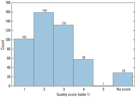
Distribution of quality scores from 1 to 5 for fundamental resonance frequency (f0) peaks from horizontal-to-vertical spectral ratio sites and the number of horizontal-to-vertical spectral ratio sites not scored.
The elevation of the Pierre Shale at selected HVSR sites along transects and at wells where HVSR data were not measured were compared to evaluate HVSR results. The wells used for comparison are shown in the inset maps of sheets 1–3 as orange squares near geophysical transects. The elevation of the Pierre Shale at nearby wells was calculated using the land-surface elevation at the well from light detection and ranging data and the depth to Pierre Shale reported in driller logs (South Dakota Department of Environment and Natural Resources, 2020). The well and HVSR site pairs were chosen using the shortest perpendicular distance between the well and its nearest HVSR site. In total, the difference in Pierre Shale elevation was calculated for 18 well and HVSR site pairs. The mean and median elevation differences were about 3.2 and 2.6 m, respectively. The minimum and maximum elevation differences in depth to bedrock were about 0.1 and 7.2 m, respectively.
The discrepancy in Pierre Shale elevation between wells and HVSR site pairs could result from (1) the perpendicular distance between wells and the nearest HVSR site along transects, (2) incorrectly reported depth to Pierre Shale in driller logs, (3) the range of depths to Pierre Shale and f0 peaks included in determining the local regression equation, (4) poor f0 peaks that were difficult to identify, and (or) (5) f0 peaks related to contacts other than unconsolidated deposits and Pierre Shale. The perpendicular distance between wells and HVSR site pairs was greater than 10 m for about 86 percent of all 18 pairs and had a maximum distance of about 76 m. The perpendicular distance likely was not responsible for the elevation differences for most well and HVSR site pairs because the slope of the bedrock surface, in most instances, would have to exceed 10–20 percent to explain the elevation discrepancy.
Another possible explanation for the elevation discrepancy is incorrectly reported depths to Pierre Shale from driller logs at wells. If the depths to Pierre Shale were reported incorrectly at wells where HVSR data were not collected, then the elevation of the Pierre Shale, calculated using light detection and ranging data, would be incorrect and a discrepancy would exist. The driller logs for each well near HVSR transects were inspected to avoid incorrect depths to Pierre Shale; however, the Pierre Shale may have been misidentified at some well sites, causing the reported depth to Pierre Shale to be incorrect. Driller logs at some wells reported clay layers directly overlying the Pierre Shale that were difficult to distinguish from the Pierre Shale and may have been reworked or weathered shale that behaves like and interacts with overlying unconsolidated deposits.
An incorrectly reported depth to Pierre Shale also would affect the local regression equation used to calculate the depth to Pierre Shale at HVSR sites along transects. The local regression equation is directly related to the reported depth to Pierre Shale because the empirical constants determined through regression would be different if incorrectly reported depths to Pierre Shale were changed. An incorrectly reported depth to Pierre Shale at HVSR was unlikely because the driller logs at each well were inspected thoroughly before they were included in analysis. The regression analysis included 13 of the 29 total HVSR well sites because sites were included only if the Pierre Shale could be clearly distinguished from overlying unconsolidated deposits in driller logs.
The local regression equation also was affected by the range in depth to Pierre Shale and f0 peaks at wells included in the regression analysis. The depth to Pierre Shale ranged from 7.0 to 13.1 m for wells included in the regression analysis. HVSR sites along transects with a true depth to Pierre Shale either greater or less than the depth range in the regression analysis may not be accurately reproduced using the local regression equation. The estimated depth to Pierre Shale at these HVSR sites, calculated using the local regression equation, might be more accurate if more data were included in the regression from a larger range of depths to Pierre Shale. The estimated depth to Pierre Shale at HVSR sites along transects outside the depth range of wells included in regression analysis may be either overestimated or underestimated.
The other factor affecting the local regression equation, and depth to Pierre Shale calculations along transects, was the f0 peaks at wells. The f0 values at wells included in the regression analysis ranged from 6.44 to 9.09 hertz; and mean and median values were 7.42 and 7.44 hertz, respectively. About 60 percent of all f0 peaks at HVSR sites along transects that produced f0 peaks were within the range of the f0 values for wells included in the regression analysis. The local regression equation may have overestimated or underestimated the depth to Pierre Shale at the remaining 40 percent of HVSR sites along transects outside the f0 range at wells included in the regression analysis.
The depth to Pierre Shale estimates calculated by the local regression equation were compared to depth to Pierre Shale calculated using equation 3 to check if the local regression equation either overestimated or underestimated the depth to Pierre Shale. The mean vs of 300.1 m/s determined at HVSR well sites and the f0 peak for HVSR sites along transects were used in equation 3 to estimate the depth to Pierre Shale. The difference in estimated depth to Pierre Shale between the local regression equation and equation 3 with mean vs was calculated by subtracting the depth estimated from the local regression equation by the depth estimated by equation 3. The mean and median differences in depth to Pierre Shale were about −0.11 and −0.22 m, respectively, and the minimum and maximum differences were about −0.54 and 2.28 m, respectively. Additionally, about 78 percent of the differences were below zero, indicating that the depth to Pierre Shale calculated using the local regression equation were typically greater than the depth to Pierre Shale calculated using equation 3 with the mean vs. The local regression equation overestimated and underestimated the depth to Pierre Shale for HVSR sites with the lowest and highest f0 values, respectively; however, the local regression equation performed well for most sites. The absolute difference in depth to bedrock between the two methods was less than 0.5 m for about 92 percent of all HVSR sites along transects.
Another possibility for the elevation discrepancy for well and HVSR site pairs was the selection of poor f0 peaks resulting from poor coupling, noise contamination, or poor acoustic impedance. Poor coupling and noise contamination were observed at several HVSR sites and often required additional filtering, which sometimes did not produce an observable f0 peak. Weak acoustic impedance contrast between clay-rich unconsolidated deposits and the Pierre Shale also likely contributed to the elevation discrepancy. The HVSR data that displayed low amplitude and broad f0 peaks (ratings of 1–2) often had the greatest disagreement in elevation of the Pierre Shale between well and HVSR site pairs (sheets 1–3).
Contacts other than that between unconsolidated deposits and the Pierre Shale also may have affected HVSR results. The f0 peaks at HVSR sites that overestimated the elevation of the Pierre Shale may have correlated with a contact between sand and gravel rich and clay-rich zones, rather than the contact between unconsolidated deposits and the Pierre Shale. The f0 peaks that underestimated the top elevation of the Pierre Shale may have correlated with the transitional contact between weathered and competent Pierre Shale and indicated a weathered zone of as much as 10.0 m thick. Driller logs from the South Dakota Department of Environment and Natural Resources (2020) that penetrated the Pierre Shale about 4.5 to 10.0 m had a transition from weathered to competent Pierre Shale.
Delineation of the Pierre Shale
The ERT and HVSR results, coupled with driller logs from nearby wells, were used to delineate the top of the Pierre Shale along 26 transects in selected areas within and near EAFB. The depth to the Pierre Shale along transects ranged from about 2.4 m (transect 4A2) to 20.3 m (transect 9A); mean and median depths were about 9.2 and 9.0 m, respectively. Table 3 shows the summary statistics for the depth to the Pierre Shale for transects in sheets 1–3. The greatest mean depth to Pierre Shale was observed (in descending order) along transects 9A, 8B, 8A, 12, 8C, and 11, where the mean depth exceeded 10.0 m. The greatest mean depth to Pierre Shale was expected along these transects because they were in the northeast part of EAFB where driller logs from wells indicated Quaternary terrace deposits were thicker than in other areas.
The lowest mean depth to Pierre Shale was observed, in ascending order, along transects 13B, 4A1, 4A2, 1C2, and 5, where the mean depth was less than 7.0 m. The lowest thickness of Quaternary terrace deposits was expected in the southern part of EAFB where the Pierre Shale crops out more frequently, and driller logs from wells show decreased thickness of Quaternary terrace deposits. Additionally, a surficial geologic map from Redden and DeWitt (2009) showed part or all of transects 13B, 4A1, 4A2, 1C2, and 5 intersected the Pierre Shale at the land surface; and many had relatively low subsurface resistivity values, minimal resistivity variation, or both. The elevation of the Pierre Shale generally increased with land-surface elevation along individual transects and from south to north within and near EAFB; however, some transects showed the Pierre Shale in topographically high and low elevation areas along transects that sometimes did not correlate with land-surface topography (sheets 1–3) and may affect local groundwater flow.
Table 3.
Summary statistics of the depth to the Pierre Shale for each of the geophysical transects shown in sheets 1–3.The elevation of the top of Pierre Shale delineated from ERT and HVSR results correlated well at the intersection of transects and with each other but had some inconsistencies. In total, 9 intersection points were observed among the 26 transects, and the delineated elevation of the Pierre Shale was within 0.3 m for all but 2 intersection points that had 0.4 m (intersection of transects 14 and 15; sheet 1) and 0.7 m (intersection of transects 2 and 3B; sheet 2) differences. The differences in elevation at intersection points were relatively small when compared to the depth to the Pierre Shale (difference between the land surface and the Pierre Shale surface), which showed that ERT and HVSR results produced a consistent Pierre Shale surface elevation.
The delineated elevation of Pierre Shale surfaces in sheets 1–3 were based mostly on ERT results that had a transition from high to low resistivity at about 30 ohm-m that correlated with the top of the Pierre Shale. The ERT results were preferred over HVSR results because the 2D models provided a more discernable and horizontally complete image of the Pierre Shale along transects; however, HVSR results were useful for filling ERT data gaps and verifying the Pierre Shale surface interpreted from ERT profiles. Driller logs from nearby wells were used to constrain the delineation of the Pierre Shale where ERT and HVSR results either underestimated or overestimated the elevation of the Pierre Shale. The underestimated or overestimated elevation of the Pierre Shale was likely from unconsolidated deposits being lithologically similar to the Pierre Shale and the weathered upper part of the Pierre Shale, resulting in minimal differences in electrical properties and a low acoustic impedance contrast for HVSR. The underestimated elevation of the Pierre Shale at some HVSR sites was likely the f0 peak occurring at the transition from weathered to unweathered Pierre Shale.
Summary
The U.S. Geological Survey, in cooperation with the U.S. Air Force Civil Engineering Center, investigated the use of surface geophysical methods to delineate the top of bedrock along survey transects in selected areas within and near Ellsworth Air Force Base (EAFB). Two complementary geophysical methods—electrical resistivity and passive seismic—were used along 26 co-located transect surveys within and near EAFB for a total of 12.7 line-kilometers. Electrical resistivity and passive seismic surveys were co-located for direct comparison and to improve interpretation of the bedrock surface. Electrical resistivity data were collected in a line-fashion to produce a two-dimensional image of subsurface resistivity, whereas passive seismic data were collected as soundings to provide a depth to bedrock at a single point. Two-dimensional electrical resistivity tomography (ERT) models were constructed for each transect using tomographic inversion software. Passive seismic data were collected and evaluated using the horizontal-to-vertical spectral ratio (HVSR) method where a local regression equation was calculated to determine the depth to bedrock.
Geophysical survey results were evaluated individually and in an integrated fashion to delineate the Pierre Shale for 26 transects within and near EAFB. It was noted that ERT results were not continuous because of a data-collection error that caused profiles to have data gaps that could not be interpreted. The range of resistivity values for ERT transects was investigated using a surficial geology map. The ERT transects mostly intersected Quaternary terrace deposits but also intersected Quaternary alluvial deposits and the Pierre Shale. The ERT inversion results of some transects showed that resistivity values of Quaternary terrace deposits generally decreased toward streams and surface contacts with other geologic units, such as the Pierre Shale. The surficial geology map showed that 15 ERT transects intersected the Pierre Shale. ERT inversion results from 9 of the 15 ERT transects showed resistivity values less than about 30 ohm-meters at or near the surface where the Pierre Shale was intersected.
The HVSR results were evaluated using a categorical rating system to assess the quality of fundamental resonance frequency (f0) peaks. The rating system scored each HVSR site on a scale of 1 (worst) to 5 (best) based on the coupling, the amplitude and width of its f0 peak, and noise contamination. HVSR results at HVSR sites with quality scores 1 and 2 accounted for about 57 percent of all sites scored, whereas HVSR sites with quality scores 3–5 accounted for about 43 percent of all sites scored. The distribution of quality scores for the HVSR sites demonstrated the variability of the acoustic impedance contrast between the Pierre Shale and overlying surficial deposits throughout the study area. The acoustic impedance contrast may have varied because of several factors, including (1) differences in the degree of weathering of the Pierre Shale, (2) lithological similarities or differences between the Pierre Shale and overlying surficial deposits, or (3) changes in the structure of the bedrock surface. The quality codes also were investigated for spatial patterns, but no observable patterns were apparent.
The elevation of the Pierre Shale at selected HVSR sites along transects and at wells where HVSR data were not measured were compared to evaluate HVSR results. The well and HVSR site pairs were chosen using the shortest perpendicular distance between the well and its nearest HVSR site. In total, the difference in Pierre Shale elevation was calculated for 18 well and HVSR site pairs. The mean and median elevation differences were about 3.2 and 2.6 m, respectively. The minimum and maximum elevation differences in depth to bedrock were about 0.1 and 7.2 m, respectively. The discrepancy in Pierre Shale elevation between well and HVSR site pairs may have resulted from (1) the perpendicular distance between wells and the nearest HVSR site along transects, (2) incorrectly reported depth to Pierre Shale at wells, (3) the range of depths to Pierre Shale and f0 peaks included in determining the local regression equation, (4) poor f0 peaks that were difficult to identify, and (or) (5) f0 peaks related to contacts other than unconsolidated deposits and Pierre Shale.
The ERT and HVSR results, coupled with driller logs from nearby wells, were used to delineate the top of the Pierre Shale along 26 transects in selected areas within and near EAFB. The depth to the Pierre Shale along transects ranged from about 2.4 m (transect 4A2) to 20.3 m (transect 9A); mean and median depths were about 9.2 m and 9.0 m, respectively. The greatest mean depth to Pierre Shale was observed, in descending order, along transects 9A, 8B, 8A, 12, 8C, and 11, where the mean depth exceeded 10.0 m. The greatest mean depth to Pierre Shale was expected along these transects because they were in the northeast part of EAFB where driller logs from wells indicated Quaternary terrace deposits were thicker than in other areas.
The lowest mean depth to Pierre Shale was observed, in ascending order, along transects 13B, 4A1 and 4A2, 1C2, and 5, where the mean depth was less than 7.0 m. The lowest thickness of Quaternary terrace deposits was expected in the southern part of EAFB where the Pierre Shale crops out more frequently, and driller logs from wells show decreased thickness of Quaternary terrace deposits. The elevation of the Pierre Shale generally increased with land-surface elevation along individual transects and from south to north within and near EAFB; however, some transects showed the Pierre Shale in topographically high and low elevation areas along transects that sometimes did not correlate with land-surface topography and may affect local groundwater flow.
The delineated elevation of Pierre Shale surfaces were based mostly on ERT results that showed a transition from high to low resistivity at about 30 ohm-meters that correlated with the top of the Pierre Shale. The ERT results were preferred over HVSR results because their two-dimensional models provided a more discernable and horizontally complete image of the Pierre Shale along transects; however, HVSR results were useful for filling ERT data gaps and verifying the Pierre Shale surface interpreted from ERT profiles. Driller logs from nearby wells were used to constrain the delineation of the Pierre Shale where ERT and HVSR results either underestimated or overestimated the elevation of the Pierre Shale. The underestimated or overestimated elevation of the Pierre Shale was likely from unconsolidated deposits being lithologically similar to the Pierre Shale and the weathered upper part of the Pierre Shale, resulting in minimal differences in electrical properties and a low acoustic impedance contrast for HVSR. The underestimated elevation of the Pierre Shale at some HVSR sites was likely the f0 peak occurring at the transition from weathered to unweathered Pierre Shale.
References Cited
Advanced Geosciences Inc, 2020, High-speed 2D/3D resistivity/IP/SP imaging system package—56 electrodes: Advanced Geosciences Inc. web page, accessed December 7, 2020, at https://www.agiusa.com/high-speed-2d3d-resistivityipsp-imaging-system-package-56-electrodes.
Bredehoeft, J.D., Neuzil, C.E., and Milly, P.C.D., 1983, Regional flow in the Dakota aquifer—A study of the role of confining layers: U.S. Geological Survey Water Supply Paper 2237, 45 p. [Also available at https://doi.org/10.3133/wsp2237.]
Constable, S.C., Parker, R.L., and Constable, C.G., 1987, Occam’s inversion—A practical algorithm for generating smooth models from electromagnetic sounding data: Geophysics, v. 52, no. 3, p. 289–300, accessed December 1, 2020, at https://doi.org/10.1190/1.1442303.
Farquharson, C.G., and Oldenburg, D.W., 1998, Non-linear inversion using general measures of data misfit and model structure: Geophysical Journal International, v. 134, no. 1, p. 213–227, accessed December 1, 2020, at https://doi.org/10.1046/j.1365-246x.1998.00555.x.
Heath, R.C., 1983, Basic ground-water hydrology: U.S. Geological Survey Water Supply Paper 2220, 86 p. [Also available at https://doi.org/10.3133/wsp2220.]
Lane, J.W., Jr., White, E.A., Steele, G.V., and Cannia, J.C., 2008, Estimation of bedrock depth using the horizontal-to-vertical (H/V) ambient-noise seismic method, in Symposium on the Application of Geophysics to Engineering and Environmental Problems, April 6–10, 2008, Philadelphia, Pa., Proceedings: Denver, Colo., Environmental and Engineering Geophysical Society, 13 p., accessed March 11, 2021, at https://water.usgs.gov/ogw/bgas/publications/SAGEEP2008-Lane_HV/.
Loke, M.H., 2004, Tutorial: 2-D and 3-D electrical imaging surveys: M.H. Loke, 157 p., accessed March 11, 2021, at https://sites.ualberta.ca/~unsworth/UA-classes/223/loke_course_notes.pdf.
Mazáč, O., Kelly, W.E., and Landa, I., 1985, A hydrogeophysical model for relations between electrical and hydraulic properties of aquifers: Journal of Hydrology (Amsterdam), v. 79, no. 1–2, p. 1–19, accessed February 2021 at https://doi.org/10.1016/0022-1694(85)90178-7.
McGregor, E.E., and Cattermole, J.M., 1973, Geologic map of the Rapid City NW quadrangle, Meade and Pennington Counties, South Dakota: U.S. Geological Survey Geologic Quadrangle 1093. [Also available at https://doi.org/10.3133/gq1093.]
Medler, C.J., Tatge, W.S., and Bender, D.A., 2021, Ellsworth Air Force Base geophysical data: U.S. Geological Survey data release, https://doi.org/10.5066/P9XSJH17.
National Earthquake Hazards Reduction Program, 2020, NEHRP recommended seismic provisions for new buildings and other structures: Washington D.C., Building Safety Council, FEMA P–2082–1, v. 1, part 1 provisions, part 2 commentary, 593 p., accessed February 23, 2021, at https://www.fema.gov/sites/default/files/2020-10/fema_2020-nehrp-provisions_part-1-and-part-2.pdf.
National Geodetic Survey, 2014, National Geodetic Survey Data Explorer—Data sheet for permanent identifier PU2524: National Oceanic and Atmospheric Administration digital data, accessed June 2016 at https://www.ngs.noaa.gov/.
Redden, J.A., and DeWitt, E., 2009, Maps showing geology, structure, and geophysics of the central Black Hills, South Dakota: U.S. Geological Survey, Scientific Investigations Map SIM–2777, scale 1:100,000, accessed March 11, 2021, at https://ngmdb.usgs.gov/ngm-bin/pdp/zui_viewer.pl?id=16864.
Rydlund, P.H., Jr., and Densmore, B.K., 2012, Methods of practice and guidelines for using survey-grade global navigation satellite systems (GNSS) to establish vertical datum in the United States Geological Survey: U.S. Geological Survey Techniques and Methods, book 11, chap. D1, 102 p., accessed April 17, 2014, at https://doi.org/10.3133/tm11D1.
Sheets, R.A., 2002, Use of electrical resistivity to detect underground mine voids in Ohio: U.S. Geological Survey Water-Resources Investigations Report 2002–4041, 33 p. [Also available at https://doi.org/10.3133/wri024041.]
South Dakota Department of Environment and Natural Resources, 2020, Water well completion reports: South Dakota Department of Environment and Natural Resources database, accessed December 7, 2020, at https://apps.sd.gov/nr68welllogs/.
U.S. Environmental Protection Agency, 2021, Superfund site: Ellsworth Air Force Base, SD: U.S. Environmental Protection Agency, accessed March 2021 at https://cumulis.epa.gov/supercpad/cursites/csitinfo.cfm?id=0800585.
U.S. Geological Survey, 2021, USGS water data for the Nation: U.S. Geological Survey National Water Information System database, accessed May 6, 2021, at https://doi.org/10.5066/F7P55KJN.
Yong, A., Thompson, E.M., Wald, D., Knudsen, K.L., Odum, J.K., Stephenson, W.J., and Haefner, S., 2016, Compilation of VS30 data for the United States: U.S. Geological Survey Data Series 978, 8 p. [Also available at https://doi.org/10.3133/ds978.]
Zohdy, A.A.R., Eaton, G.P., and Mabey, D.R., 1974, Application of surface geophysics to groundwater investigations: U.S. Geological Survey Techniques of Water-Resources Investigations, book 2, chap. D1, 116 p., accessed March 11, 2021, at https://doi.org/10.3133/twri02D1.
Conversion Factors
Datum
Vertical coordinate information is referenced to the North American Vertical Datum of 1988 (NAVD 88)
Horizontal coordinate information is referenced to the North American Datum of 1983 (NAD 83)
For more information about this publication, contact:
Director, USGS Dakota Water Science Center
821 East Interstate Avenue, Bismarck, ND 58503
1608 Mountain View Road, Rapid City, SD 57702
605–394–3200
For additional information, visit: https://www.usgs.gov/centers/dakota-water
Publishing support provided by the
Rolla Publishing Service Center
Suggested Citation
Medler, C.J., and Anderson, T.M., 2021, Delineating the Pierre Shale from geophysical surveys within and near Ellsworth Air Force Base, South Dakota, 2019: U.S. Geological Survey Scientific Investigations Map 3474, 3 sheets, 16-p. pamphlet, https://doi.org/10.3133/sim3474.
ISSN: 2329-132X (online)
Study Area
| Publication type | Report |
|---|---|
| Publication Subtype | USGS Numbered Series |
| Title | Delineating the Pierre Shale from geophysical surveys within and near Ellsworth Air Force Base, South Dakota, 2019 |
| Series title | Scientific Investigations Map |
| Series number | 3474 |
| DOI | 10.3133/sim3474 |
| Year Published | 2021 |
| Language | English |
| Publisher | U.S. Geological Survey |
| Publisher location | Reston, VA |
| Contributing office(s) | Dakota Water Science Center |
| Description | Pamphlet: ix,16 p.; 3 Sheets: 48.00 x 40.00 inches or smaller; Data Release; Dataset |
| Country | United States |
| State | South Dakota |
| Other Geospatial | Ellsworth Air Force Base |
| Online Only (Y/N) | Y |
| Google Analytic Metrics | Metrics page |