

Maps of Elevation of Top of Pierre Shale and Surficial Deposit Thickness with Hydraulic Properties from Borehole Geophysics and Aquifers Tests within and near Ellsworth Air Force Base, South Dakota, 2020–21
Links
- Document: Pamphlet (2.12 MB pdf) , HTML , XML
- Sheets:
- Sheet 1 (10.9 MB pdf) —Map showing elevation contours of the top of Pierre Shale from well logs and electrical resistivity tomography data
- Sheet 2 (7.83 MB pdf) —Map showing contours of depth to Pierre Shale, hydraulic conductivity, and groundwater velocity of surficial deposits
- Dataset: USGS National Water Information System database —USGS water data for the Nation
- Data Releases:
- USGS data release —Datasets used to create maps of Pierre Shale elevation and surficial deposit thickness within and near Ellsworth Air Force Base, South Dakota, 2021
- USGS data release —Electrical resistivity tomography (ERT) and horizontal-to-vertical spectral ratio (HVSR) data collected within and near Ellsworth Air Force Base, South Dakota, from 2014 to 2019
- Download citation as: RIS | Dublin Core
Acknowledgments
The authors thank the U.S. Air Force Civil Engineer Center for funding assistance and Ellsworth Air Force Base, the South Dakota Ellsworth Development Authority, and private landowners for providing access to field sites and wells.
This work was supported in part by the U.S. Geological Survey Water Mission Area Hydrogeophysics Branch. The authors also thank Carole Johnson (Observing Systems Division, Hydrologic Remote Sensing Branch) and Randall Bayless (Ohio-Kentucky-Indiana Water Science Center) for guidance and expertise for geophysical data collection. Additionally, the authors thank the U.S. Geological Survey reviewers for their careful analysis and comments.
Abstract
The U.S. Geological Survey, in cooperation with the U.S. Air Force Civil Engineer Center, collected borehole geophysical data and completed simple aquifer tests to estimate the thickness and hydraulic properties of surficial deposits. The purpose of data collection was to create generalized contour maps of the elevation of the top of the Pierre Shale and the thickness of overlying surficial deposits within and near Ellsworth Air Force Base (study area). Natural gamma and electromagnetic induction data were collected to refine or determine surficial deposit thickness at selected wells. Additionally, data from previous geophysical studies and driller logs were compiled and combined with results from natural gamma and electromagnetic induction data to provide a more spatially complete image of the subsurface. Borehole nuclear magnetic resonance (bNMR) data were collected to estimate hydraulic conductivity and water content of surficial deposits overlying Pierre Shale. Simple aquifer tests using water slugs (slug tests) were completed to estimate hydraulic conductivity of surficial deposits, and results were compared to hydraulic conductivity estimates from bNMR data. All data used to construct maps and estimate hydraulic properties are provided in an accompanying U.S. Geological Survey data release (available at https://doi.org/10.5066/P9FLR79F).
Generalized contour maps were constructed using results from 26 borehole geophysical logs, 35 geophysical transects from previous studies, and 304 wells with driller logs. The elevation of the top of the Pierre Shale generally followed land-surface topography, sloping from high elevations in the north to lower elevations in the south. Topographic highs of Pierre Shale, where present, could act as groundwater divides that potentially affect groundwater flow direction. Surficial deposit thickness varied spatially and ranged from 0 to 86 feet. Surficial deposits generally were thickest in higher elevation areas near ephemeral streams in the northern part of the study area. Hydraulic conductivity estimated from bNMR results using two analytical methods ranged from 0.1 to 2,314 feet per day, whereas hydraulic conductivity estimated from slug tests ranged from 0.001 to 193 feet per day. Hydraulic conductivity estimates from slug tests were plotted with surficial deposit thickness contours instead of bNMR estimates because bNMR estimates were determined to overestimate hydraulic conductivity. Hydraulic conductivity values generally were greater in the southwestern part of study area than the northeastern part.
Introduction
Ellsworth Air Force Base (EAFB; study area) is 6 miles east of Rapid City, South Dakota, next to the town of Box Elder, and includes about 4,860 acres of land (fig. 1). EAFB began operating in 1942 and, as of 2022, the base manages runway, airfield, and aircraft maintenance operations with supporting industrial areas, housing units, and recreational facilities. More than 80 years of operations at the base caused contamination of soil, sediment, surface water, and groundwater on base and on private lands outside base boundaries (U.S. Environmental Protection Agency, 2022). From 1985 to 1989, the U.S. Air Force began investigating possibly contaminated sites by collecting soil and water samples. In 1990, the base was included on the U.S. Environmental Protection Agency National Priorities List, and cleanup efforts began at the base. Remediation efforts at EAFB are regulated by the U.S. Environmental Protection Agency and the State of South Dakota (U.S. Environmental Protection Agency, 2022).
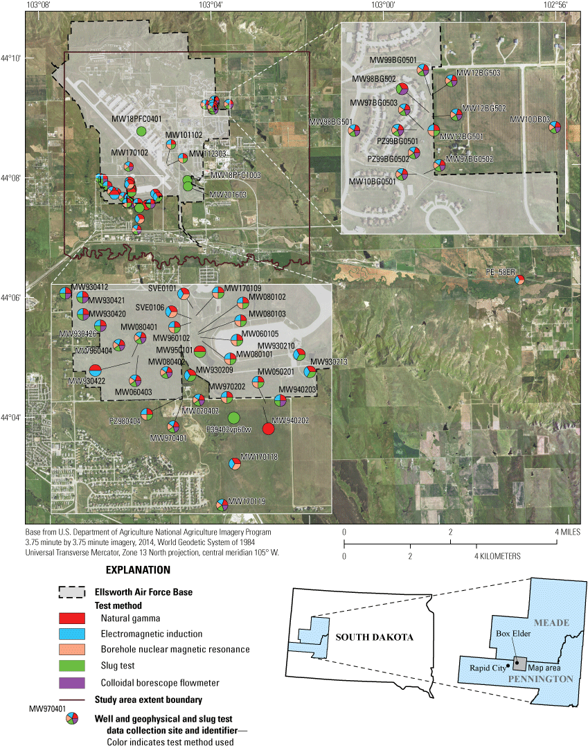
South Dakota Department of Agriculture and Natural Resources (2022) wells where borehole geophysical data and aquifer (slug) tests were completed within and near Ellsworth Air Force Base, South Dakota.
The direction and magnitude of groundwater flow through surficial deposits are necessary data for tracking and (or) intercepting contaminant migration within and near EAFB. Surficial deposits in the study area are defined as any unconsolidated deposits overlying the Cretaceous Pierre Shale and are primarily Quaternary alluvial and terrace deposits consisting of a mixture of clay, silt, sand, and gravel (Redden and DeWitt, 2008; Medler and Anderson, 2021). Other surficial deposits in the study area include material added or removed during EAFB operations, such as remediation of landfills or excavation for construction. The Cretaceous Pierre Shale is a dark gray to black marine shale with low hydraulic conductivity (Redden and DeWitt, 2008) and is the uppermost bedrock unit in the study area. The Cretaceous Pierre Shale may affect groundwater flow patterns in areas where the topography of its buried surface differs from the topography of the land surface.
The U.S. Geological Survey (USGS), in cooperation with the U.S. Air Force Civil Engineer Center, collected borehole geophysical data and completed simple aquifer tests to estimate the thickness and hydraulic properties of surficial deposits. Contour maps of the elevation of the top of the Pierre Shale and thickness of overlying surficial deposits with hydraulic properties were created for the study area (fig. 1). Borehole geophysical techniques and aquifer tests provide a means of characterizing hydrogeologic conditions to supplement existing information from published geophysical surveys and driller logs. Natural gamma and electromagnetic induction (EMI) data were collected to refine or determine surficial deposit thickness at selected wells. Borehole nuclear magnetic resonance (bNMR) data were collected to estimate hydrologic properties, such as hydraulic conductivity and water content, of surficial deposits. Aquifer tests using water slugs (slug tests) were completed to estimate hydraulic conductivity of surficial deposits. Additionally, the USGS tested the usefulness of colloidal borescope flowmeter (CBFM) logging for determining the horizontal flow direction and velocity of groundwater within and near EAFB (appendix 1). Maps of the elevation of the top of the Pierre Shale and thickness of surficial deposits with hydraulic conductivity estimates could assist remediation managers in estimating the movement of groundwater and contaminants in the study area.
Purpose and Scope
The purpose of this report is to provide maps of the elevation of the top of the Pierre Shale (sheet 1; available for download at https://doi.org/10.3133/sim3502) and thickness of overlying surficial deposits with hydraulic conductivity estimates (sheet 2; available for download at https://doi.org/10.3133/sim3502) near EAFB. The scope of this report is to document data collection procedures and provide the results of borehole geophysical surveys and slug tests completed from July 2020 to August 2021 at wells in the study area. Generalized contour maps were constructed to better understand groundwater flow and contaminant transport in the study area. Borehole geophysical data were collected to refine or determine the thickness of surficial deposits and estimate hydrologic properties. Slug tests were completed in most wells where borehole geophysical data were collected, and hydraulic conductivity estimates from slug tests were compared to estimates from bNMR logs. In total, borehole geophysical and slug test data were collected at 45 and 44 wells, respectively. Contour maps of the elevation of the top of the Pierre Shale (sheet 1) and thickness of surficial deposits (sheet 2) in the study area were created using data from borehole geophysical logs, published geophysical surveys, and driller logs. Additionally, hydraulic conductivity estimates from slug tests were plotted with surficial deposit thickness (sheet 2).
Methods for Determining Pierre Shale Elevation, Surficial Deposit Thickness, and Hydraulic Conductivity of Surficial Deposits
Generalized contour maps of Pierre Shale elevation and surficial deposit thickness were constructed using data from borehole geophysical logs, published geophysical surveys, and driller logs. Borehole geophysical techniques included natural gamma, EMI, and bNMR (fig. 1). Additionally, CBFM data were collected in the study area, and results and conclusions are discussed in appendix 1. Previous geophysical data from Medler and Anderson (2021) and Medler (2022) and lithologic information from wells with driller logs (South Dakota Department of Agriculture and Natural Resources, 2022) were combined with borehole geophysical logs to provide a more spatially complete image of the subsurface in the study area. The bNMR logs and results from aquifer tests using water slugs (slug tests) were used to determine hydrologic properties of surficial deposits in the study area. The well name, USGS National Water Information System site number (U.S. Geological Survey, 2022a), latitude, longitude, elevation, and geophysical method for each well visited for data collection are listed in table 1. A complete list of wells included in construction of maps is available in the accompanying USGS data release (Medler and others, 2022).
Table 1.
Observation wells within and near Ellsworth Air Force Base, South Dakota, where borehole geophysical data and aquifer tests (slug tests) were completed from July 2020 to August 2021 with site information, including latitude, longitude, elevation, and measuring point height.[USGS, U.S. Geological Survey; NAVD 88, North American Vertical Datum of 1988; MP, measuring point; LS, land surface; EMI, electromagnetic induction; bNMR, borehole nuclear magnetic resonance; CBFM, colloidal borescope flowmeter; x, denotes method used; --, no data or not applicable]
| Well name1 | USGS site number2 | Latitude, in decimal degrees | Longitude, in decimal degrees | Elevation, in feet above NAVD 88 | MP height, in feet above LS | Borehole geophysical method | Slug test | |||
|---|---|---|---|---|---|---|---|---|---|---|
| Natural gamma | EMI | bNMR | CBFM (appendix 1) | |||||||
| MW020402 | 440731103055401 | 44.12552 | −103.09949 | 3,133.60 | 2.82 | x | x | x | x | x |
| MW050201 | 440730103053301 | 44.12516 | −103.09311 | 3,131.99 | 2.72 | x | x | x | -- | x |
| MW060105 | 440752103055214 | 44.12969 | −103.09905 | 3,165.29 | 2.72 | x | x | x | -- | x |
| MW060403 | 440737103061103 | 44.12848 | −103.10541 | 3,150.52 | 2.67 | x | x | x | x | x |
| MW080101 | 440752103055217 | 44.12944 | −103.09889 | 3,153.44 | 2.82 | x | x | x | -- | x |
| MW080102 | 440752103055218 | 44.13003 | −103.09922 | 3,171.59 | 2.99 | x | x | x | -- | x |
| MW080103 | 440752103055202 | 44.12990 | −103.09926 | 3,166.50 | 2.66 | x | x | x | -- | x |
| MW080401 | 440743103061701 | 44.12859 | −103.10489 | 3,153.94 | 2.75 | x | x | x | x | x |
| MW080402 | 440738103061101 | 44.12739 | −103.10226 | 3,146.00 | 2.75 | x | x | x | x | x |
| MW101102 | 440811103050701 | 44.13649 | −103.08532 | 3,179.46 | 2.92 | x | x | x | -- | x |
| MW10BG501 | 440904103035901 | 44.15116 | −103.06690 | 3,181.33 | 2.87 | x | x | x | x | x |
| MW10OB03 | 440909103033901 | 44.15256 | −103.06071 | 3,181.99 | 2.92 | x | x | x | x | x |
| MW112303 | 440809103050601 | 44.13588 | −103.08492 | 3,178.77 | 2.59 | x | x | x | -- | x |
| MW12BG501 | 440909103035801 | 44.15258 | −103.06625 | 3,185.66 | 2.62 | x | x | x | -- | x |
| MW12BG502 | 440911103035801 | 44.15299 | −103.06619 | 3,186.88 | 2.62 | x | x | x | x | x |
| MW12BG503 | 440913103035801 | 44.15358 | −103.06619 | 3,191.99 | 2.67 | x | x | x | x | x |
| MW170102 | 440809103055701 | 44.13583 | −103.09917 | 3,194.32 | 2.43 | x | x | x | x | x |
| MW170109 | 440752103055901 | 44.13111 | −103.09972 | 3,189.99 | 2.17 | x | x | x | -- | x |
| MW170118 | 440720103054501 | 44.12124 | −103.09618 | 3,123.00 | 2.07 | x | x | x | -- | -- |
| MW170119 | 440705103055001 | 44.11821 | −103.09739 | 3,068.01 | 1.97 | x | x | x | x | x |
| MW18PFC0401 | 440844103054101 | 44.14557 | −103.09467 | 3,212.00 | 0.30 | -- | -- | -- | -- | x |
| MW18PFC1003 | 440756103044101 | 44.13166 | −103.07733 | 3,113.79 | 0.00 | -- | -- | -- | -- | x |
| MW201603 | 440747103043801 | 44.12995 | −103.07713 | 3,118.66 | −0.20 | -- | -- | -- | -- | x |
| MW930209 | 440738103060001 | 44.12716 | −103.10006 | 3,147.57 | 2.99 | x | x | -- | -- | x |
| MW930210 | 440741103062001 | 44.12812 | −103.10563 | 3,147.44 | 2.88 | x | x | -- | -- | x |
| MW930213 | 440738103052001 | 44.12722 | −103.08894 | 3,115.19 | 2.68 | x | x | -- | -- | x |
| MW930412 | 440800103064102 | 44.13285 | −103.11114 | 3,202.66 | 2.79 | x | x | -- | x | x |
| MW930420 | 440754103063601 | 44.13166 | −103.10986 | 3,190.04 | 2.06 | x | x | -- | x | x |
| MW930421 | 440752103062802 | 44.13254 | −103.10988 | 3,200.23 | 2.70 | x | x | -- | x | x |
| MW930422 | 440741103062001 | 44.12812 | −103.10563 | 3,147.44 | 2.88 | x | x | -- | -- | -- |
| MW930426 | 440752103062804 | 44.13065 | −103.10829 | 3,178.54 | 2.42 | x | x | -- | x | x |
| MW940203 | 440731103053001 | 44.12533 | −103.09176 | 3,135.38 | 2.61 | x | x | -- | x | x |
| MW950101 | 440743103055701 | 44.12873 | −103.09912 | 3,160.41 | 2.48 | x | -- | -- | -- | x |
| MW960102 | 440751103055902 | 44.13083 | −103.09972 | 3,175.98 | 2.82 | x | x | x | -- | x |
| MW960404 | 440745103062401 | 44.12906 | −103.10665 | 3,154.30 | 2.92 | x | x | x | x | x |
| MW970202 | 440732103054800 | 44.12561 | −103.09669 | 3,125.17 | 2.53 | x | x | x | -- | x |
| MW970401 | 440737103055204 | 44.12554 | −103.10084 | 3,134.02 | 2.59 | x | x | x | x | x |
| MW97BG0502 | 440904103040001 | 44.15115 | −103.06658 | 3,179.46 | 2.71 | x | x | x | x | x |
| MW97BG0503 | 440909103040001 | 44.15260 | −103.06656 | 3,185.10 | 2.49 | x | x | x | x | x |
| MW98BG501 | 440909103041100 | 44.15261 | −103.06968 | 3,193.86 | 2.79 | x | x | x | x | x |
| MW98BG502 | 440911103035901 | 44.15319 | −103.06632 | 3,188.89 | 3.18 | x | -- | -- | x | x |
| MW99BG0501 | 440913103035802 | 44.15369 | −103.06616 | 3,191.99 | 3.54 | x | x | x | x | x |
| P39402vp60w | 440727103054601 | 44.12424 | −103.09610 | 3,117.14 | −0.35 | -- | -- | -- | -- | x |
| PE–58ER | 440606102570001 | 44.10178 | −102.94989 | 2,930.68 | 2.53 | x | x | x | -- | -- |
| PZ980404 | 440733103060302 | 44.12582 | −103.10095 | 3,134.35 | 2.79 | x | x | x | -- | x |
| PZ99BG0501 | 440909103040101 | 44.15258 | −103.06687 | 3,186.65 | 2.92 | x | x | x | x | x |
| PZ99BG0502 | 440907103040101 | 44.15185 | −103.06701 | 3,183.01 | 3.21 | x | x | x | x | x |
| SVE0101 | 440751103055904 | 44.13083 | −103.09972 | 3,189.96 | 2.92 | x | x | x | -- | -- |
| SVE0106 | 440751103055901 | 44.13083 | −103.09972 | 3,182.19 | 3.00 | x | x | x | -- | -- |
Well names from the South Dakota Department of Agriculture and Natural Resources (2022).
Well number in the U.S. Geological Survey National Water Information System database (U.S. Geological Survey, 2022a).
Borehole Geophysical Techniques
Borehole geophysical techniques used in this study included natural gamma, EMI, and bNMR. Borehole geophysical data were collected at 45 wells in the study area from September 2020 to August 2021. Wells chosen for borehole geophysical logging were selected based on location, access, well-construction materials, and the condition of the well casing and screen. Wells were selected to cover as much of the study area as possible but were restricted to wells belonging only to EAFB or the State of South Dakota. Well-construction materials were examined from driller logs (South Dakota Department of Agriculture and Natural Resources, 2022), if available, or during field visits to ensure wells with metal casing and screens were excluded because the EMI and bNMR probes are sensitive to metal in the wellbore. In some cases, driller logs were not available or did not specify the casing and screen material, so the EMI probe was used to determine the casing and screen material before bNMR data collection. The bNMR probe cannot be used in wells with metal components or construction materials because the probe could be damaged during data collection if metal is present. Data collected using the EMI probe in wells with metal casings and (or) screens were not included in the analysis. Natural gamma data were collected at wells with metal casings and (or) screens because the casing and screen material do not affect the probe. The condition of the well casing and screen was examined during field visits, and a Waterra pump (Waterra Pumps Limited, 2022) was used to clear sediment from well screens.
Methods for each borehole geophysical method, including physics, instruments, and analysis, are described in the following sections. Additional background information for geophysical methods is provided by Keys (1990) and Hearst and others (2000). All borehole geophysical data are provided in the accompanying data release (Medler and others, 2022) and in the USGS GeoLog Locator system (U.S. Geological Survey, 2022b).
Natural Gamma Logging
Natural gamma logging measures the total amount of gamma radiation emitted by materials surrounding a borehole (Keys, 1990). Two Mount Sopris Instruments (MSI) 2PGA–1000 polygamma tools were used to collect natural gamma logs. Gamma radiation is measured by the MSI 2PGA–1000 tool using a sodium iodide crystal that emits a pulse of light when struck with a gamma ray, which is then amplified and converted to a current pulse. Naturally occurring sources of gamma radiation commonly include potassium-40 and daughter products of the uranium and thorium-decay series (Johnson and others, 2011). Shales commonly contain higher fractions of radioactive minerals than other rock types, which produce higher gamma counts. Gamma logs can be used to differentiate geologic units and lithology, especially shale bedrock. The vertical resolution of the MSI 2PGA–1000 tool is about 0.3 to 0.6 meter (Johnson and others, 2011). A more complete background on gamma logging is provided by Keys (1990).
Gamma tools are calibrated by manufacturers to American Petroleum Institute units; however, tool calibration drifts over time and the data collected in American Petroleum Institute units may not be accurate (Johnson and others, 2011). Instead, tools can be operated so that natural gamma data are measured in units of counts per second. Natural gamma data collected during this study were measured in units of counts per second because the tools had not been calibrated by manufacturers since they were constructed. Additionally, two MSI 2PGA–1000 tools that likely were manufactured at different times were used in this study, and the drift rate of each tool was likely different; therefore, gamma emissions measured in counts per second from two or more tools were evaluated to ensure the tools were measuring similarly. Multiple wells were selected for repeat measurements where both tools were used to collect natural gamma data. The gamma data from repeat measurements indicated both tools measured gamma variations similarly, and therefore, no correction was needed.
Field procedures used for natural gamma log data collection in the “down” and “up” directions using the MSI 2PGA–1000 tool are described in this section. Before the gamma tool was inserted in a well, the depth to water and depth to bottom of the well were measured using an electric water-level tape using procedures described in Cunningham and Schalk (2011). Next, the tool was connected to a winch system that recorded the depth and speed at which the tool moved in the well. Additionally, a laptop was connected to the winch system to monitor data collection. The tool was then inserted in the well, and top of the probe was leveled to the top of casing (either above or below land surface). The probe was then turned on and lowered at a constant speed of about 10 feet per minute while collecting data until the tool reached near the bottom of the well. After recording and saving the log file, the tool was raised at a constant speed of about 10 feet per minute until the top of the tool reached the top of casing.
Natural gamma log data were collected at 45 wells in September 2020 and from July to August 2021. Natural gamma log data were processed using MSI WellCAD software (https://mountsopris.com/wellcad/). Before interpretation, natural gamma log data were depth corrected to land surface by subtracting the casing stickup, if applicable, from the depths recorded by the winch system so the depth to the top of the Pierre Shale (equivalent to surficial deposit thickness) was comparable among wells. After depth corrections were applied, a three-point moving-average filter was used to suppress data variations and produce a smooth log to document larger scale gamma count variations correlating to lithologic changes. Moving-average filters can introduce error by shifting the depths of gamma count measurements up or down. The depth error introduced from the three-point moving-average filter used in this study did not affect interpretation because the error was less than the vertical resolution of the tool. Depth corrected and filtered natural gamma data are available in the data release accompanying this report (Medler and others, 2022). Lithologic information from driller logs (South Dakota Department of Agriculture and Natural Resources, 2022), if available, was used to constrain interpretations of natural gamma logs. The Pierre Shale was expected to produce a higher gamma count than overlying surficial deposits, even those consisting mostly of clay and silt, because of its high content of radioactive minerals (Schultz and others, 1980).
Electromagnetic Induction Logging
EMI logging measures the bulk electrical conductivity (in millisiemens per meter) of materials and fluids in materials surrounding a borehole (Williams and others, 1993). An MSI 2PIA–1000 tool was used to collect EMI logs in this study. The EMI tool generates an electromagnetic field to induce an electrical current in the materials surrounding the borehole. The induced current then generates a secondary electromagnetic field that is measured as a voltage in receiver coils in the tool. Electrical conductivity is determined by the tool because it is proportional to the strength of the secondary electromagnetic field measured by the receiver coils when induction numbers are low (less than 100 millisiemens per meter; McNeill, 1986). Electrical conductivity changes are caused by borehole construction and the composition of materials and fluids surrounding the borehole, such as borehole diameter, casing material (steel, polyvinyl chloride, and so on), porosity of materials, specific conductance of groundwater, and the abundance of metallic minerals in materials. The effect of water in the borehole on electrical conductivity measurements is minimized because the tool was designed to be most sensitive to materials and groundwater about 1 foot (ft) away from the borehole (Johnson and others, 2011). Although the EMI tool measures electrical conductivity variations, the data file from the tool also reports electrical resistivity, the reciprocal of electrical conductivity, and is commonly plotted with electrical conductivity on composite geophysical logs. The vertical resolution of the tool is about 2 ft. A more complete background on EMI logging is provided by McNeill (1986).
The MSI 2PIA–1000 tool was calibrated before each measurement following procedures provided by the manufacturer. First, the tool was powered on and lowered into the borehole until it was either fully or partially submerged in the borehole fluids for 15–20 minutes to stabilize and equilibrate the internal temperature of the tool. Second, the tool was removed from the borehole and calibrated using two-point calibration with a free-air value of zero and (or) a calibration ring with the dial set at 465 or 2,060 millisiemens per meter based on the expected range of electrical conductivity values at each site. The two-point calibration involved holding the tool vertically in the air either with or without the calibration ring and was completed as quickly as possible to avoid major thermal changes. At some wells, the two-point calibration could not be completed because of tool malfunctions and was instead operated at “full scale” using manufacturer settings. EMI logs collected when operating at “full scale” were evaluated at three wells using two EMI tools—one calibrated and the other at “full scale.” The EMI logs from the calibrated and “full scale” tools were nearly identical and indicated minor variations. The tool was submerged for 15–20 minutes in the borehole fluid when the “full scale” settings were used to minimize thermal effects on data collection.
EMI log data were collected at 43 wells from July to August 2021. EMI log data were processed using MSI WellCAD software (https://mountsopris.com/wellcad/). Before interpretation, EMI log data were depth corrected to land surface from the depths recorded by the winch system so the depth to the top of the Pierre Shale (equivalent to surficial deposit thickness) was comparable among wells. After depth corrections were applied, a two-point moving-average filter was used to suppress variations and produce a smooth log to document larger scale variations correlating to lithologic and (or) groundwater chemistry. Moving-average filters can introduce error by shifting the depths of electrical conductivity measurements up or down. The depth error introduced from the two-point moving-average filter used in this study did not affect interpretation because the error was less than the vertical resolution of the tool. Depth corrected and filtered EMI data are available in the data release accompanying this report (Medler and others, 2022). Lithologic information from driller logs (South Dakota Department of Agriculture and Natural Resources, 2022) and natural gamma logs, if available, were used to constrain interpretations of EMI logs. The Pierre Shale was expected to produce higher electrical conductivity values than overlying surficial deposits because of its relatively high clay content and saline groundwater (Schultz and others, 1980; Williamson and Carter, 2001).
Borehole Nuclear Magnetic Resonance Logging
The bNMR logging estimates the water content, pore-size distribution, and hydraulic conductivity of materials in the saturated zone surrounding a borehole. Either a Javelin JP–175 or JP–238 logging tool, both manufactured by Vista Clara, Inc. (Walsh and others, 2013), was used to collect bNMR logs depending on the diameter of the well casing. The JP–175 and JP–238 have a diameter of 1.75 inches (in.) and 2.38 in., respectively, and were used to collect data in 2-in. and 6-in. diameter wells, respectively. The JP–175 tool was used for bNMR data collection for all wells, except wells SVE0101 and SVE0106, where the JP–238 tool was used because the wells had a 6-in. diameter casing. Both bNMR tools use static magnets and radio frequency fields to estimate hydraulic properties of a thin shell (0.08 in. thick) of material surrounding a borehole at a specific distance (7.5 in. for the JP–175 and 11.5 in. for the JP–238) from the borehole. Static magnets in the tool cause water molecules in the geologic material surrounding the tool to align to the magnetic field generated by the tool. The tool emits radio frequency fields to disrupt the magnetic field and cause the protons in the water molecule to be tipped into the transverse plane normal to the background field. The bNMR tool then measures the strength of the magnetic field produced as protons in the water molecules undergo precession to the background magnetic field imposed by the static magnets before disruption from radio frequencies. The signal strength decreases exponentially with time and is called the transverse relaxation time (T2). In these measurements, the initial magnetic field strength in the T2 is directly proportional to the total water content in the measurement zone. In saturated sediments, the total water content is equivalent to the formation porosity. The rate of the T2 indicates the pore-size distribution; faster T2 indicates smaller pore sizes and slower T2 indicates larger pore sizes. The echo spacing, the time between each pulse during the measurement, for the JP–175 and JP–238 are 1.0 and 1.2 milliseconds, respectively. Additional background on bNMR tools used for this study is provided by Walsh and others (2013).
The bNMR data were collected at 34 wells from July to August 2021 using Javelin JP–175 or JP–238 tools. The diameter of the drilled borehole and the screened interval were reviewed in driller logs for each well, if available, before data collection to ensure the measurement zone of the tool was outside of the drilled hole and in surficial deposits overlying the Pierre Shale. Measurements in packing material within the drilled hole and the Pierre Shale were not the focus of this study and were removed where possible when collecting bNMR data; however, in some cases, bNMR data were collected within the disturbed zone of the borehole and (or) in wells screened entirely in the Pierre Shale. Additionally, bNMR data were not collected in the unsaturated zone of each well because hydraulic conductivity and pore-size distribution can be estimated only in the saturated zone.
At each site, the water level and total depth of each well were measured using an electric water-level tape. Next, the tool was connected to a winch system that recorded the depth and speed at which the tool moves in the well. Additionally, a laptop was connected to the winch system to monitor data collection. The tool then was inserted in the well and referenced to the top of casing (either above or below land surface). The bNMR data were collected in the up direction at 1.6-ft intervals in the saturated zone of the well starting from the bottom of the well. Dual-frequency measurements were made at center frequencies of about 300 and 250 kilohertz. Additionally, two relaxation times were used for both tools: a full relaxation time of 4 seconds and a shorter “burst-mode” relaxation time of 1 second. Measurements were stacked 30 times for the full relaxation time and 180 times for the burst-mode relaxation time.
The bNMR data were processed using the manufacturer-supplied software, VC_Javelin_Processor, version 4.1.1. In postprocessing, the full and burst-mode measurements for each frequency were combined for each 1.6-ft depth increment. An impulse noise filter was used to remove noisy T2 data. The bNMR data also were adjusted by removing the ambient noise collected with an external reference coil measured concurrently with the subsurface measurements. The resultant T2 data from the combined frequencies was fit with a multiexponential decay curve, which was inverted to produce a pore-size distribution model. For each depth, the pore-size distribution was determined as a fraction of the total water content. For each depth interval, the total, mobile, capillary, and clay fractions were determined using empirically derived cutoff T2 values (Straley and others, 1997). The total water content includes the mobile and immobile fractions of water, which consist of the capillary and clay fractions. The mobile fraction, which is the fraction that decays after the 33-millisecond cutoff, represents the effective porosity. The immobile fraction, which includes the clay and capillary fractions that decay before the 33-millisecond cutoff, represents bound water. The clay-fraction cutoff was set at a T2 value of 3 milliseconds.
Hydraulic conductivity estimates from bNMR data were calculated using default parameters in VC_Javelin_Processor software (version 4.1.1) with two equations: (1) the Schlumberger-Doll research (SDR) equation (Kenyon and others, 1988) and (2) the sum of echoes (SOE) equation (Allen and others, 2000). The SDR equation uses the measured values of total porosity and the mean log T2, as follows:
whereKsdr
is the SDR hydraulic conductivity, in meters per day;
C
is an empirically derived constant that was set to the default parameter of 8,900;
ϕ
is total porosity;
m
is an empirically derived constant that is generally about 1 for unconsolidated sands (Behroozmand and others, 2015);
MLT2
is the mean log T2; and
n
is an empirically derived constant fixed at 2 (Grunewald and others, 2014).
Ksoe
is the SOE hydraulic conductivity, in meters per day;
C
is an empirically derived constant set to 4,200; and
SE
is the measured sum of echoes (Grunewald and others, 2014).
Previous Geophysical Surveys and Driller Logs
Previous geophysical surveys and wells with driller logs containing lithologic information were used to construct generalized maps of the elevation of the top of the Pierre Shale (sheet 1) and thickness of surficial deposits (sheet 2) in the study area. Medler and Anderson (2021) and Medler (2022) delineated nearly continuous profiles of the elevation of the top of the Pierre Shale within and near EAFB along two-dimensional survey transects chosen in areas with little or no wells using electrical resistivity tomography and passive seismic techniques. The latitude and longitude of survey transects were determined from a real-time kinematic survey using methods described by Rydlund and Densmore (2012). For consistency, the elevation along each transect was determined using a light detection and ranging (lidar) digital elevation dataset with a vertical accuracy of 0.4 ft at 95 percent confidence (City of Rapid City, 2015). Pierre Shale elevation, latitude, longitude, and elevation of each site along transects are available as data releases (Medler and others, 2021, 2022).
In addition to geophysical surveys, wells with driller logs containing lithologic information also were used to construct sheets 1 and 2. Driller logs were obtained from the South Dakota Department of Agriculture and Natural Resources (2022) and from data provided by EAFB (Rita Krebs, Ellsworth Air Force Base, written commun., 2021). Latitude and longitude for each well site were surveyed by either the USGS or by EAFB and verified using EAFB records, information from previous reports, and photographic imagery. Land-surface elevation of each site along survey transects was determined using the same lidar digital elevation dataset as previous geophysical surveys. Lithologic information from driller logs was inspected for each well to either verify or reinterpret the thickness of surficial deposits reported in the driller log. Only wells that penetrated the Pierre Shale were used because the total thickness of surficial deposits was desired for the generalized thickness contour map. A complete list of the wells—including the latitude, longitude, and elevation of each well site—used to construct the generalized thickness contour map are included in the accompanying data release (Medler and others, 2022).
Surficial deposit thickness derived from geophysical logs identifying the top of the Pierre Shale in table 2 were combined with thicknesses at other wells and geophysical transects (Medler and Anderson, 2021; Medler, 2022) to construct generalized contour maps of the elevation of the top of the Pierre Shale (sheet 1) and thickness of surficial deposits (sheet 2) in the study area. The elevation of the top of the Pierre Shale was calculated by subtracting the depth to shale from the land-surface elevation. The land-surface elevation was extracted from a 1-meter resolution digital elevation model created from lidar data (City of Rapid City, 2015). Interpolation of the Pierre Shale elevation from the wells and geophysical transects was completed using the Topo to Raster tool in ArcGIS Pro (Esri, 2019). The interpolated raster was contoured and manually adjusted to correct for areas of sparse data. The contours were considered inferred when farther than 1,000 ft from the wells or geophysical transects used to interpret the depth to Pierre Shale. A thickness raster of the surficial deposits overlying the Pierre Shale was created by subtracting the elevation raster of the top of the Pierre Shale from the digital elevation model of the land surface. The thickness raster was contoured and considered inferred when farther than 1,000 ft from the wells and geophysical transects used to interpret the Pierre Shale elevation. Shape files of the contours are available in the accompanying data release (Medler and others, 2022).
Table 2.
Thickness of surficial deposits from driller logs and (or) delineated using borehole geophysical logs for 45 wells in the study area.[URL, Uniform Resource Locator]
Well names from the South Dakota Department of Agriculture and Natural Resources (2022).
Slug Tests
Slug tests were completed from July 10, 2020, to September 3, 2020, at 44 wells (table 1) to estimate hydraulic properties of surficial deposits in the study area. A slug test is a type of aquifer test that estimates hydraulic conductivity of aquifer materials close to a well by measuring the subsequent rise or fall of the water level in a well in response to a nearly instantaneous change in hydraulic head (Butler, 2020). Slug test durations were less than 60 minutes and often less than 20 minutes; therefore, atmospheric changes during the tests did not affect data collection and test results. About 2 to 5 days before slug tests, wells were developed by removing sediment and material in the well screens to improve hydrologic connection between the well screen and the aquifer. Well development was completed by pumping the well for as many as 30 minutes with a surge block and Waterra pump (Waterra Pumps Limited, 2022). Water levels were measured before and after well development to ensure groundwater in the wells returned to equilibrium before starting the slug test.
Data Collection for Slug Tests
Data collected for slug test analysis included well-construction information, general aquifer characteristics, and water-level changes recorded during each test. Driller logs, when available (table 2; Medler and others, 2022), provided various well-construction information and general aquifer characteristics including lithologic descriptions, well-screen length, well-construction material, inside radius of the well casing, and the well borehole diameter. Well-construction information such as total well depth and measuring-point height for each well was verified by electric water-level tape and a surveyor tape, respectively, using methods described by Cunningham and Schalk (2011). Wells without driller logs (table 2) were examined in the field for well-construction material (normally polyvinyl chloride) and inside radius of the well (normally 1 in.). Wells without borehole diameter information were assumed completed with a 4.25-in. radius auger based on wells constructed similarly during the same year. Additionally, geophysical logs were used to determine the well-screen length and screened interval for wells without driller logs by identifying the depth of the bentonite plug or seal in the annular space of the well using high gamma counts in natural gamma logs. Specific well-construction data and general aquifer characteristics used for slug test analysis are available in the accompanying data release (Medler and others, 2022).
Water levels were measured before slug testing with a calibrated electric water-level tape (Cunningham and Schalk, 2011). Water levels were used to determine saturated thickness and the depth to suspend a submersible transducer below the water surface to record water levels before and during the slug test. The transducer was an unvented Solinst Levelogger LT F30/M10 (https://www.solinst.com/) with a radius of 0.036 ft. The transducer was suspended between 2 and 6 ft below the water surface and was the only downhole equipment in the well. The transducer recorded at 1-second intervals, and water levels were corrected for barometric pressure using a Solinst Barologger LT F15/M5 (https://www.solinst.com/) placed within 50 ft of the well during the slug test. The anisotropy ratio (vertical to horizontal hydraulic conductivity ratio, Kz/Kr, where Kz is vertical hydraulic conductivity and Kr is horizontal hydraulic conductivity) was assumed to be 0.1, which is a common value for unconsolidated sediments (Freeze and Cherry, 1979). Water-level data collected during slug tests are available in the accompanying data release (Medler and others, 2022).
Water slugs were used rather than solid slugs to prevent cross contamination between wells. The water slug also ensured a rapid head displacement in the well during the slug test. One to three slug test trials were completed at each well with differing volumes of water for each trial; the first trial used 0.5 liter (L) of water, the second trial used 1.0 L, and the third trial used 1.5 L. Water-level response during slug testing was variable among the wells; some tests recovered in less than 1 minute but other tests did not fully recover within 60 minutes. If water-level recovery times exceeded 20 minutes, only one trial was completed. Water-level displacement was calculated by subtracting the barometrically corrected water level from a reference (static) water level. The reference (static) water level was equal to the median of 30 consecutive seconds of stable barometrically corrected water-level data recorded by the transducer before or after the slug test.
Sampling intervals for some slug test trials were edited to ensure an appropriate and manageable number of data points for analysis because some slug test trials recorded as many as 60 minutes (more than 3,000 data points) of water-level data. Editing the sampling interval also reduced “noisy” data caused by spurious water-level data points. Python programming language (van Rossum and Drake, 2011) was used to edit the sampling interval of water-level data for trials exceeding 30 seconds. The initial 30 seconds of data during each trial were retained, and the sampling interval was changed for the remaining data based on the total water-level recovery time of the trial: one data point every 30 seconds was retained for slug test trials exceeding 1,000 seconds, one point every 20 seconds was retained for trials between 500 and 1,000 seconds, one data point every 10 seconds was retained for trials between 200 and 500 seconds, and one point every 5 seconds was retained for trials between 30 and 200 seconds. Editing the sampling rate did not affect analysis because the largest water-level displacement changes were within the first 30 seconds of the trials, and edited sampling rates were applied when water-level changes were relatively small.
Analytical Methods for Slug Tests
Water-level changes for each slug test trial were analyzed with AQTESOLV Pro, version 4.50.002 (Hydrosolve, Inc., 2007), using the Kansas Geological Survey (KGS; Hyder and others, 1994) method for unconfined aquifers without well skin. The KGS method was selected because the method best represents well conditions in the study area. The method incorporates the storage properties of the well and general aquifer characteristics, such as saturated thickness (Butler, 2020). Additionally, the KGS model considers the effects of partial well penetration into the aquifer and aquifer anisotropy (Hyder and others, 1994).
AQTESOLV uses curve fitting to provide an estimate of hydraulic conductivity and specific storage. The curve-fitting algorithm creates a best-fit curve by varying the estimated hydraulic conductivity and other hydrogeologic parameters until a theoretical curve best fits the measured time and water-level observations (Hydrosolve, Inc., 2007). The automatic curve-fitting feature in AQTESOLV using the KGS method without well skin was used for all slug test trials. AQTESOLV-readable files used for analysis are available in the accompanying data release (Medler and others, 2022). Although calculated by AQTESOLV, estimates of specific storage using the KGS method were not reported because of the questionable accuracy of storage and specific storage estimates from slug tests (Butler, 2020). Storage is the ability of an aquifer to accept or release water over time, and changes in storage can take considerable time; therefore, the short water-level recovery time and the small volume of the aquifer tested by the slug tests resulted in uncertain storage estimates for this study.
Geophysical Logging and Slug Test Results
Geophysical logging and slug test results were used to estimate the thickness and hydraulic properties of surficial deposits in the study area. Thickness of surficial deposits was delineated using a combination of natural gamma logs, EMI logs, and lithologic information from driller logs. Hydraulic conductivity and water content estimates were calculated from bNMR data collected at 30 wells. Slug tests provided estimates of hydraulic conductivity at 44 wells completed in the surficial deposits and the Pierre Shale. Hydraulic conductivity estimates from bNMR data and slug tests were compared and evaluated spatially to highlight relatively higher conductivity values that indicate areas of preferential groundwater flow.
Pierre Shale Elevation and Surficial Deposit Thickness from Borehole Geophysical Logs, Previous Geophysical Surveys, and Driller Logs
Composite geophysical logs were constructed for 34 of the 45 total wells where natural gamma, EMI, and bNMR data were collected together (table 1). Composite geophysical logs were not constructed for the remaining 11 wells because gamma, EMI, and bNMR data were not collectively measured at those wells (fig. 1); however, when possible, the thickness of surficial deposits was delineated for wells where natural gamma and (or) EMI logs were collected. In total, surficial deposit thickness was successfully delineated for 26 of 45 wells using borehole geophysical logs (table 2). A composite geophysical log for well PE–58ER is provided in figure 2 as an example of how the depth to the top of the Pierre Shale (equivalent to surficial deposit thickness) was delineated for this study. The top of the Pierre Shale generally had greater gamma counts on natural gamma logs and lower electrical resistivity values on EMI logs compared to overlying surficial deposits; for example, high count natural gamma zones were identified from 2 to 7 ft and from 23 to 25 ft below land surface in figure 2. High natural gamma counts from 2 to 7 ft were attributed to the bentonite seal shown in figure 2, whereas the zone from 23 to 25 ft corresponded to the top of Pierre Shale. The EMI log showed minor variation with decreasing electrical resistivity toward the contact with the Pierre Shale at 23.5 ft (fig. 2).
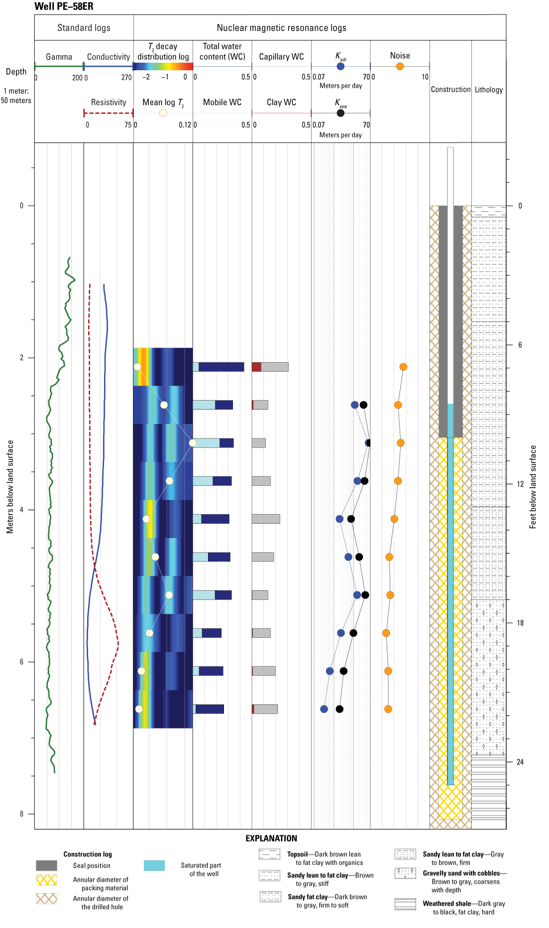
Borehole geophysical logs for well PE–58ER, including natural gamma, electromagnetic induction, and borehole nuclear magnetic resonance logs with well-construction and lithology information from the accompanying driller log. Borehole nuclear magnetic resonance data provided measurements of water content and estimates of hydraulic conductivity. The amplitude color plot shows the distribution of the transverse relaxation time (T2). The total and mobile water content and clay and capillary content are shown to the right of the color amplitude plot as bar plots with values expressed as a fractional number. [Ksdr, hydraulic conductivity estimated using Schlumberger-Doll research equation; Ksoe, hydraulic conductivity estimated using the sum of echoes equation]
Surficial deposit thickness could not be determined from borehole geophysical logs for 19 of 45 wells (table 2) because either the well did not penetrate the Pierre Shale or lithologic similarities between surficial deposits and the Pierre Shale prevented contact delineation. Lithologic information from driller logs, if available, was used to determine surficial deposit thickness for wells lacking natural gamma and electrical resistivity trends consistent with the Pierre Shale. Surficial deposit thickness was unknown at wells MW170102, MW930422, MW98BG502, and MW99BG0501 (table 2) because composite geophysical logs did not indicate patterns consistent with Pierre Shale and driller logs were not available.
Reported thickness of surficial deposits from driller logs was compared to thickness estimates from borehole geophysical logs for 15 wells (table 2). The absolute difference between reported thicknesses from driller logs and thicknesses delineated using borehole geophysical logs ranged from 0 to 7.6 ft, and differences were less than or equal to 2 ft for 12 of the 15 wells (table 2). Lithologic similarities between surficial deposits and weathering of the upper part of the Pierre Shale made identification of the contact imprecise, which likely contributed to thickness differences from driller logs and borehole geophysical logs exceeding 2 ft at 3 of the 15 wells (table 2).
Surficial deposit thickness from borehole geophysical logs in table 2 was combined with thicknesses from geophysical transects (Medler and Anderson, 2021; Medler, 2022) and other wells to construct generalized contour maps of the elevation of the top of the Pierre Shale (sheet 1) and thickness of surficial deposits (sheet 2) in the study area. A complete list of wells and geophysical transects used in construction of sheets 1 and 2 is included in the accompanying data release (Medler and others, 2022). In total, 35 geophysical transects and 330 wells were used to construct sheets 1 and 2.
The elevation of the top of the Pierre Shale generally followed land-surface topography, sloping from high elevations in the north to lower elevations in the south (sheet 1). Topographic highs of Pierre Shale, where present, could act as groundwater divides that potentially affect groundwater flow direction. Surficial deposit thickness varied throughout the study area and ranged from 0 to 86 ft. The thickness of the surficial deposits generally was less than 20 ft in areas where the surficial deposits are incised by ephemeral stream valleys (sheet 2). Thicknesses likely are exaggerated in areas with roads or infrastructure that artificially increased the land-surface elevation. Surficial deposits generally were thickest in higher elevation areas near ephemeral streams in the northern part of the study area (sheet 2).
Hydraulic Conductivity and Water Content from Borehole Nuclear Magnetic Resonance Results
Hydraulic conductivity and water content were estimated from bNMR logs for 30 of the 34 wells with composite geophysical logs (table 3; Medler and others, 2022). Hydraulic conductivity was calculated using the SDR (eq. 1) and SOE (eq. 2) equations only for bNMR data collected in the saturated part of surficial deposits. Water content was estimated in the saturated and unsaturated parts of surficial deposits. In the saturated zone, the water content is equal to porosity. Electrical interference and (or) dry well conditions prevented estimation of hydraulic conductivity and water content at wells MW170102, MW170118, PZ980404, and PZ99BG0501 and at various measurement depths at other wells.
Table 3.
Hydraulic conductivity and water content estimates computed using the Schlumberger-Doll research and sum of echoes equations on borehole nuclear magnetic resonance data for 34 wells in the study area.[SDR, Schlumberger-Doll research; SOE, sum of echoes; --, no data or not applicable]
An example of bNMR results for well PE–58ER is shown in figure 2. The T2 measurements are shown as a color amplitude plot where the x-axis is the relaxation time of the T2 measurement in units of log seconds). The amplitude of the water content is shown for each depth as a function of color; the warm colors (red) indicate high amplitude and cool colors (blue) indicate low amplitude. High amplitudes on the left side of the T2 plot indicate short relaxation times consistent with water in small pore spaces, such as those in silt and clay. High amplitudes on the right side of the T2 plot indicate long relaxation times, consistent with water in larger pore spaces. The water content fractions at each depth measured are split into total and mobile and clay and capillary (immobile). The bNMR log in the unsaturated zone from about 6 ft below land surface to water (8.5 ft in fig. 2) is characterized by a high total water content fraction at about 0.40 and contains as much as 0.10 as clay content and 0.20 as capillary content.
Hydraulic conductivity estimates for all bNMR measurements ranged from 0.1 to 2,314 feet per day (ft/d) for equation 1 (SDR) and 0.1 to 874 ft/d for equation 2 (SOE; Medler and others, 2022). The range of hydraulic conductivity values estimated from bNMR data generally was within the range of expected values representative of silty sand to gravel (0.1 to 8,000 ft/d; Heath, 1983; Domenico and Schwartz, 1990). Mean and median hydraulic conductivity values for all bNMR measurements were 237 and 48 ft/d and 167 and 107 ft/d for equations 1 and 2, respectively (Medler and others, 2022). At most wells, mean and median hydraulic conductivity values estimated using equation 1 (SDR) were smaller than values estimated using equation 2 (SOE; table 3). The largest differences between hydraulic conductivities estimated using equations 1 and 2 were, in decreasing order, at wells SVE0106, MW050201, MW020402, and MW970202 (table 3). Well-construction effects on bNMR logs were evident for most wells in the study because the drilled diameter of most wells (8.5–10.25 in.) was greater than the radius of investigation (7.5 in. for JP–175) of the bNMR tool.
Comparison of hydraulic conductivity estimates from equations 1 and 2 indicated that estimates from equation 1 (SDR) were more subject to variations caused by noise in the mean log T2 value than were estimates from equation 2 (SOE). Although equation 2 is less sensitive to noise, equation 1 can better indicate small variations in hydraulic conductivity caused by fine materials detected by the early-time T2 measurement. The estimates from equations 1 and 2 indicated similar patterns of low and high hydraulic conductivity, although the magnitude of the estimated hydraulic conductivity values at various depths differed by as much as a factor of 20.
The bNMR tool also measured water content, including the mobile and immobile fractions, of the unsaturated and saturated zones surrounding boreholes. The mean total water content across the 30 sites in table 3 ranged from 0.25 to 0.46. The mean mobile water content (or effective porosity) ranged from 0.02 to 0.32 (table 3). The low mobile water content of surficial deposits in the study area was attributed to the high clay content of the deposits noted from driller logs.
Hydraulic Conductivity Estimates from Slug Tests
Hydraulic conductivity estimates from slug tests are listed in table 4. Most wells were screened in the surficial deposits overlying the Pierre Shale; however, seven wells were screened entirely or partially in the Pierre Shale. Hydraulic conductivity estimates from slug tests for all 81 trials for wells completed in surficial deposits ranged from 0.001 to 193 ft/d, and mean and median hydraulic conductivity estimates were 25 and 9 ft/d, respectively. The mean hydraulic conductivity for an individual well ranged from 0.001 ft/d at MW12BG503 to 134 ft/d at MW080402. Hydraulic conductivity estimates for the nine trials completed at wells screened entirely or partially in the Pierre Shale ranged from 0.04 at MW060105 to 0.9 ft/d at MW080102, and mean and median hydraulic conductivity estimates were 0.3 and 0.09 ft/d, respectively. The range of hydraulic conductivity estimates for surficial deposits generally was within the range of hydraulic conductivity values representative of silty sand to gravel (0.1 to 8,000 ft/d; Heath, 1983; Domenico and Schwartz, 1990). Hydraulic conductivity estimates for the Pierre Shale generally were within the range of estimates for shale or silt (10−7 to 10−1; Heath, 1983).
Table 4.
Hydraulic conductivity estimates from slug tests for 44 wells in the study area.[--, no data or not applicable]
Mean hydraulic conductivity estimates from slug tests were plotted spatially with contours of surficial deposit thickness for spatial evaluation (sheet 2). Slug test hydraulic conductivity estimates generally were greater in the southwestern part of the study area than the northeastern part. The northeastern part of the study area is close to infrastructure (fig. 1) and may consist of compacted fill from human development near roads, infrastructure, and the runway environment, which could explain the relatively lower hydraulic conductivities measured in the northeast than in the southwest.
Comparison of Hydraulic Conductivity Estimates from Borehole Nuclear Magnetic Resonance Logs and Slug Tests
Mean hydraulic conductivity estimates for 28 wells with results from bNMR logging and slug tests were compared (fig. 3). The SDR and SOE mean hydraulic conductivity estimates from bNMR results were greater than estimates from slug tests for 14 of 27 wells and 15 of 28 wells, respectively (fig. 3). The SDR mean hydraulic conductivity of well PZ980404 could not be calculated; therefore, only 27 wells were included for comparison of the SDR estimates (fig. 3). The SDR and SOE estimates ranged from 3.0 to 56,000 and 1.1 to 78,000 times greater, respectively, than slug test estimates. Additionally, estimates from the SDR equation were greater than 10 times (one log scale on fig. 3) the estimates from slug tests for 14 of 27 wells, and estimates from the SOE equation were greater than 10 times the estimates from slug tests for 16 of 28 wells.
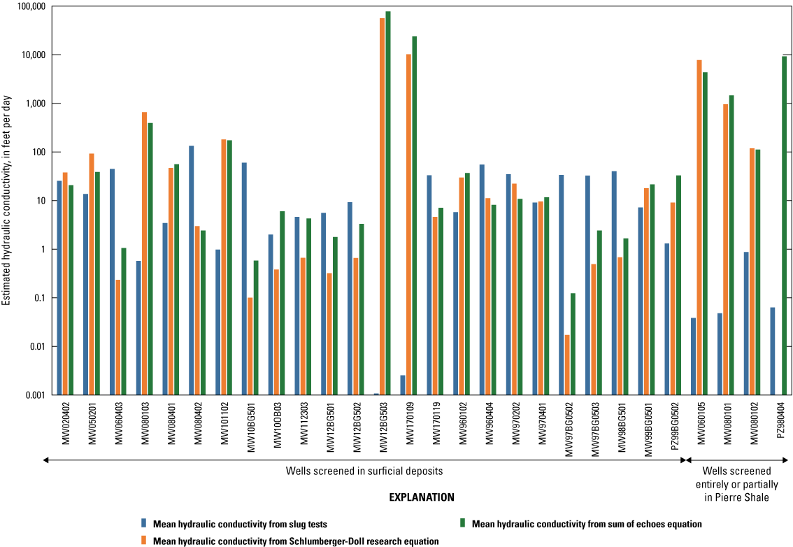
Mean hydraulic conductivity estimates from borehole nuclear magnetic resonance logging (Schlumberger-Doll research equation and sum of echoes equation) and slug test results for 28 wells.
The largest differences in mean hydraulic conductivity between SDR and SOE estimates and slug test estimates were from wells MW12BG503 and MW170109 (fig. 3), which both had the lowest estimated mean hydraulic conductivity from slug tests (table 4). Slug test data from MW12BG503 and MW170109 indicated some of the longest recovery times of all wells tested, and it is possible the well screens could be plugged despite purging before slug testing. Wells screened entirely or partially in the Pierre Shale also indicated large differences in estimated mean hydraulic conductivity. Estimates from the SDR and SOE equations ranged from 118 to 7,700 times and 111 to 9,200 times greater, respectively, than estimates from slug tests.
Mean hydraulic conductivity differences between bNMR and slug tests were attributed to differences in data collection methodology and parameters used in analysis. The bNMR logging estimated hydraulic conductivity of material at a specific radius surrounding wells and at several depth intervals, which were combined to compute a mean hydraulic conductivity of the well profile. The bNMR logging also does not consider the well screen for calculation of hydraulic conductivity. Slug testing estimates hydraulic conductivity by evaluating the water column response to increases or decreases in hydraulic head from insertion or removal of a slug, and the condition of the well screen affects the results. Therefore, hydraulic conductivity estimates calculated from bNMR data may have evaluated a different part of the aquifer near the wells than the slug tests. Additionally, well-screen conditions, such as sediments trapped in the screen, may have affected slug test results and contributed to differences in estimated mean hydraulic conductivity. The parameters used to calculate hydraulic conductivity also may have contributed to overestimation of hydraulic conductivity for bNMR data, which was observed in previous studies (Hull and others, 2019; Kendrick and others, 2021). The default parameters for T2 cutoff times were empirically derived (Straley and others, 1997) and may not accurately represent materials in the study area.
Summary
The U.S. Geological Survey, in cooperation with the U.S. Air Force Civil Engineer Center, collected borehole geophysical data and completed simple aquifer tests to estimate the thickness and hydraulic properties of surficial deposits. Contour maps of the elevation of the top of the Pierre Shale and thickness of overlying surficial deposits were created for areas within and near Ellsworth Air Force Base (study area). Borehole geophysical data were collected at 46 wells, and logging methods included natural gamma, electromagnetic induction, colloidal borescope flowmeter, and borehole nuclear magnetic resonance (bNMR). Borehole geophysical data were combined with well-construction and lithologic information from driller logs to aid interpretation of the thickness of surficial deposits. Natural gamma and electromagnetic induction data were used to estimate thickness of surficial deposits, whereas colloidal borescope flowmeter and bNMR data were used to estimate hydrologic properties of surficial deposits. Hydrologic properties also were estimated analytically using water-level changes from slug tests. All data used to construct maps and estimate hydraulic properties are provided in an accompanying U.S. Geological Survey data release (available at https://doi.org/10.5066/P9FLR79F).
Surficial deposit thickness was successfully delineated for 26 of 45 wells using geophysical logs. Surficial deposit thickness could not be determined from borehole geophysical logs for 19 of 45 wells because either the well did not penetrate the Pierre Shale or lithologic similarities between surficial deposits and the Pierre Shale prevented contact delineation. Lithologic information from driller logs, if available, was used to determine surficial deposit thickness for wells lacking natural gamma and electrical resistivity trends consistent with the Pierre Shale. Reported thickness of surficial deposits from driller logs was compared to thickness estimates from geophysical logs for 15 of those 26 wells. The absolute difference between reported thicknesses from driller logs and thicknesses delineated using geophysical logs ranged from 0 to 7.6 feet (ft), and differences were less than or equal to 2 ft for 12 of the 15 wells.
Surficial deposit thickness from the 26 borehole geophysical logs was combined with thicknesses from 35 geophysical transects and 304 wells with driller logs to construct generalized contour maps of the elevation of the top of the Pierre Shale and thickness of surficial deposits in the study area. In total, 35 geophysical transects and 330 wells were used to construct the two contour maps. The elevation of the top of the Pierre Shale generally followed land-surface topography, sloping from high elevations in the north to lower elevations in the south. Topographic highs of Pierre Shale, where present, could act as groundwater divides that potentially affect groundwater flow direction. Surficial deposit thickness varied throughout the study area and ranged from 0 to 86 ft. Surficial deposits generally were thickest in higher elevation areas near ephemeral streams in the northern part of the study area.
Hydraulic conductivity and water content were estimated from bNMR results for 30 of the 34 wells. Hydraulic conductivity estimates for all bNMR measurements ranged from 0.1 to 2,314 feet per day (ft/d) and 0.1 to 874 ft/d for equations 1 (Schlumberger-Doll research equation) and 2 (sum of echoes equation), respectively. Mean and median hydraulic conductivity values for all 140 bNMR measurements at 30 wells were 237 and 48 ft/d and 167 and 107 ft/d for equations 1 and 2, respectively. Comparison of hydraulic conductivity estimates from equations 1 and 2 indicates that estimates from equation 1 were more subject to variations caused by noise in the mean log transverse relaxation time (known as T2) value than equation 2. The mean total water content across the 30 sites ranged from 0.25 to 0.46. The mean mobile water content (or effective porosity) ranged from 0.02 to 0.32.
Slug tests were completed at 44 wells to estimate hydraulic properties of surficial deposits and the Pierre Shale. Hydraulic conductivity estimates from slug tests for wells completed in surficial deposits ranged from 0.001 to 193 ft/d, and mean and median hydraulic conductivity estimates were 25 and 9 ft/d, respectively. The mean hydraulic conductivity for an individual well ranged from 0.001 ft/d at MW12BG503 to 134 ft/d at MW080402. Hydraulic conductivity estimates for wells screened entirely or partially in the Pierre Shale ranged from 0.04 ft/d at MW060105 to 0.9 ft/d at MW080102, and mean and median hydraulic conductivity estimates were 0.3 and 0.09 ft/d, respectively. The range of hydraulic conductivity estimates for surficial deposits was generally within the range of hydraulic conductivity values representative of silty sand to gravel. Hydraulic conductivity estimates for the Pierre Shale generally were within the range of estimates for shale or silt.
References Cited
Allen, D., Flaum, C., Ramakrishnan, T.S., Bedford, J., Castelijns, K., Fairhurst, D., Gubelin, G., Heaton, N., Minh, C.C., Norville, M.A., Seim, M.R., Pritchard, T., and Ramamoorthy, R., 2000, Trends in NMR logging: Oilfield Review, v. 12, no. 3, art. OIREE70923–1730, 19 p., accessed March 2022 at https://www.ux.uis.no/~s-skj/NMR/Schlumberger/O0_CMR_OilRev.pdf.
Behroozmand, A.A., Keating, K., and Auken, E., 2015, A review of the principles and applications of the NMR technique for near-surface characterization: Surveys in Geophysics, v. 36, no. 1, p. 27–85. [Also available at https://doi.org/10.1007/s10712-014-9304-0.]
Cunningham, W.L., and Schalk, C.W., comps., 2011, Groundwater technical procedures of the U.S. Geological Survey: U.S. Geological Survey Techniques and Methods, book 1, chap. A1, 151 p., accessed December 2020 at https://doi.org/10.3133/tm1A1.
Esri, 2019, How Topo To Raster works: Esri web page, accessed December 2022 at https://pro.arcgis.com/en/pro-app/latest/tool-reference/3d-analyst/how-topo-to-raster-works.htm#:~:text=Topo%20to%20Raster%20interpolates%20elevation,streams%20from%20input%20contour%20data.
Grunewald, E., Knight, R., and Walsh, D., 2014, Advancement and validation of surface nuclear magnetic resonance spin-echo measurements of T2: Geophysics, v. 79, no. 2, p. EN15–EN23, accessed March 2022 at https://doi.org/10.1190/geo2013-0105.1.
Heath, R.C., 1983, Basic ground-water hydrology: U.S. Geological Survey Water-Supply Paper 2220, 86 p. [Also available at https://doi.org/10.3133/wsp2220.]
Hull, R.B., Johnson, C.D., Stone, B.D., LeBlanc, D.R., McCobb, T.D., Phillips, S.N., Pappas, K.L., and Lane, J.W., Jr., 2019, Lithostratigraphic, geophysical, and hydrogeologic observations from a boring drilled to bedrock in glacial sediments near Nantucket sound in East Falmouth, Massachusetts: U.S. Geological Survey Scientific Investigations Report 2019–5042, 27 p., accessed December 2022 at https://doi.org/10.3133/sir20195042.
Hyder, Z., Butler, J.J., Jr., McElwee, C.D., and Liu, W., 1994, Slug tests in partially penetrating wells: Water Resources Research, v. 30, no. 11, p. 2945–2957, accessed February 2021 at https://doi.org/10.1029/94WR01670.
Hydrosolve, Inc., 2007, AQTESOLV for Windows, version 4.5 user’s guide: Reston, Va., 529 p., accessed October 2020 at http://www.aqtesolv.com/download/aqtw20070719.pdf.
Johnson, C.D., Mondazzi, R.A., and Joesten, P.K., 2011, Borehole geophysical investigation of a formerly used defense site, Machiasport, Maine, 2003–2006: U.S. Geological Survey Scientific Investigations Report 2009–5120, 75 p. plus 6 appendixes. [Also available at https://doi.org/10.3133/sir20095120.]
Kendrick, A.K., Knight, R., Johnson, C.D., Liu, G., Knobbe, S., Hunt, R.J., and Butler, J.J., Jr., 2021, Assessment of NMR logging for estimating hydraulic conductivity in glacial aquifers: Ground Water, v. 59, no. 1, p. 31–48. [Also available at https://doi.org/10.1111/gwat.13014.]
Kenyon, W.E., Day, P.I., Straley, C., and Willemsen, J.F., 1988, A three-part study of NMR longitudinal relaxation properties of water-saturated sandstones: SPE Formation Evaluation, v. 3, no. 3, p. 622–636, accessed March 2022 at https://doi.org/10.2118/15643-PA.
Keys, W.S., 1990, Borehole geophysics applied to ground-water investigations: U.S. Geological Survey Techniques of Water-Resources Investigations, book 2, chap. E2, 149 p. [Also available at https://doi.org/10.3133/twri02E2.]
Medler, C.J., 2022, Delineating the Pierre Shale from geophysical surveys east of Box Elder, South Dakota, 2021: U.S. Geological Survey Scientific Investigations Map 3497, 3 sheets, 15-p. pamphlet, accessed December 2022 at https://doi.org/10.3133/sim3497.
Medler, C.J., and Anderson, T.M., 2021, Delineating the Pierre Shale from geophysical surveys within and near Ellsworth Air Force Base, South Dakota, 2019: U.S. Geological Survey Scientific Investigations Map 3474, 3 sheets, 16-p. pamphlet, accessed December 2022 at https://doi.org/10.3133/sim3474.
Medler, C.J., Eldridge, W.G., Anderson, T.M., and Phillips, S.N., 2022, Datasets used to create maps of Pierre Shale elevation and surficial deposit thickness within and near Ellsworth Air Force Base, South Dakota, 2021: U.S. Geological Survey data release, accessed December 2022 at https://doi.org/10.5066/P9FLR79F.
Medler, C.J., Tatge, W.S., and Bender, D.A., 2021, Electrical resistivity tomography (ERT) and horizontal-to-vertical spectral ratio (HVSR) data collected within and near Ellsworth Air Force Base, South Dakota, from 2014 to 2019: U.S. Geological Survey data release, accessed December 2022 at https://doi.org/10.5066/P9XSJH17.
Redden, J.A., and DeWitt, E., 2008, Maps showing geology, structure, and geophysics of the central Black Hills, South Dakota: U.S. Geological Survey, Scientific Investigations Map SIM–2777, scale 1:100,000, accessed March 11, 2021, at https://ngmdb.usgs.gov/ngm-bin/pdp/zui_viewer.pl?id=16864.
Rydlund, P.H., Jr., and Densmore, B.K., 2012, Methods of practice and guidelines for using survey-grade global navigation satellite systems (GNSS) to establish vertical datum in the United States Geological Survey: U.S. Geological Survey Techniques and Methods, book 11, chap. D1, 102 p., accessed January 28, 2022, at https://doi.org/10.3133/tm11D1.
Schultz, L.G., Tourtelot, H.A., Gill, J.R., and Boerngen, J.G., 1980, Composition and properties of the Pierre Shale and equivalent rocks, northern Great Plains region: U.S. Geological Survey Professional Paper 1064–B, 86 p., 1 plate. [Also available at https://doi.org/10.3133/pp1064B.]
South Dakota Department of Agriculture and Natural Resources, 2022, Water well completion reports: South Dakota Department of Agriculture and Natural Resources digital data, accessed February 2022 at https://apps.sd.gov/nr68welllogs/.
Straley, C., Rossini, D., Vinegar, H.J., Tutunjian, P.N., and Morriss, C.E., 1997, Core analysis by low field NMR: The Log Analyst, v. 38, no. 2, p. 84–94, accessed March 2022 at https://onepetro.org/petrophysics/article-abstract/170927/Core-Analysis-By-Low-field-Nmr?redirectedFrom=fulltext.
U.S. Environmental Protection Agency, 2022, Superfund site—Ellsworth Air Force Base, South Dakota cleanup activities: U.S. Environmental Protection Agency web page, accessed February 2022 at https://cumulis.epa.gov/supercpad/SiteProfiles/index.cfm?fuseaction=second.Cleanup&id=0800585#bkground.
U.S. Geological Survey, 2022a, USGS water data for the Nation: U.S. Geological Survey National Water Information System database, accessed February 2022 at https://doi.org/10.5066/F7P55KJN.
U.S. Geological Survey, 2022b, GeoLog Locator: U.S. Geological Survey digital data, accessed September 2022 at https://doi.org/10.5066/F7X63KT0.
Walsh, D., Turner, P., Grunewald, E., Zhang, H., Butler, J., Reboulet, E., Knobbe, S., Christy, T., Lane, J.W., Jr., Johnson, C.D., Munday, T., and Fitzpatrick, A., 2013, A small-diameter NMR logging tool for groundwater investigations: Groundwater, v. 51, no. 6, 12 p. [Also available at https://doi.org/10.1111/gwat.12024.]
Waterra Pumps Limited, 2022, Waterra groundwater sampling pump for monitoring wells and piezometers: Waterra Pumps Limited web page, accessed February 2022 at https://waterra.com/waterra-groundwater-sampling-pump/.
Williams, J.H., Lapham, W.W., and Barringer, T.H., 1993, Application of electromagnetic logging to contamination investigations in glacial sand and gravel aquifers: Ground Water Monitoring and Remediation, v. 13, no. 3, p. 129–138. [Also available at https://doi.org/10.1111/j.1745-6592.1993.tb00082.x.]
Williamson, J.E., and Carter, J.M., 2001, Water-quality characteristics in the Black Hills area, South Dakota: U.S. Geological Survey Water-Resources Investigations Report 2001–4194, 196 p. [Also available at https://doi.org/10.3133/wri20014194.]
Appendix 1. Colloidal Borescope Flowmeter Logging
References Cited
Geotech Environmental Equipment, Incorporated, 2021, Geotech colloidal borescope—Installation and operation manual: Geotech Environmental Equipment, Incorporated, 49 p, accessed February 2022 at https://www.geotechenv.com/Manuals/Geotech_Colloidal_Borescope.pdf.
Kearl, P.M., and Roemer, K., 1998, Evaluation of groundwater flow directions in a heterogeneous aquifer using the colloidal borescope: Advances in Environmental Research, v. 2, no. 1, p. 12–23, accessed February 2022 at https://www.geotechenv.com/pdf/white_papers/advances_in_environmental_research.pdf.
Medler, C.J., Eldridge, W.G., Anderson, T.M., and Phillips, S.N., 2022, Datasets used to create maps of Pierre Shale elevation and surficial deposit thickness within and near Ellsworth Air Force Base, South Dakota, 2021: U.S. Geological Survey data release, accessed December 2022 at https://doi.org/10.5066/P9FLR79F.
Wilson, J.T., Mandell, W.A., Paillet, F.L., Bayless, E.R., Hanson, R.T., Kearl, P.M., Kerfoot, W.B., Newhouse, M.W., and Pedler, W.H., 2001, An evaluation of borehole flowmeters used to measure horizontal ground-water flow in limestones of Indiana, Kentucky, and Tennessee, 1999: U.S. Geological Survey Water-Resources Investigations Report 2001–4139, 129 p. [Also available at https://doi.org/10.3133/wri014139.]
Conversion Factors
U.S. customary units to International System of Units
International System of Units to U.S. customary units
Datum
Vertical coordinate information is referenced to the North American Vertical Datum of 1988 (NAVD 88).
Horizontal coordinate information is referenced to the North American Datum of 1983 (NAD 83).
Elevation, as used in this report, refers to distance above the vertical datum.
Abbreviations
bNMR
borehole nuclear magnetic resonance
CBFM
colloidal borescope flowmeter
EAFB
Ellsworth Air Force Base
EMI
electromagnetic induction
KGS
Kansas Geological Survey
lidar
light detection and ranging
MSI
Mount Sopris Instruments
SDR
Schlumberger-Doll research
SOE
sum of echoes
T2
transverse relaxation time
USGS
U.S. Geological Survey
For more information about this publication, contact:
Director, USGS Dakota Water Science Center
821 East Interstate Avenue, Bismarck, ND 58503
1608 Mountain View Road, Rapid City, SD 57702
605–394–3200
For additional information, visit: https://www.usgs.gov/centers/dakota-water
Publishing support provided by the
Rolla Publishing Service Center
Suggested Citation
Medler, C.J., Eldridge, W.G., Anderson, T.M., and Phillips, S.N., 2023, Maps of elevation of top of Pierre Shale and surficial deposit thickness with hydraulic properties from borehole geophysics and aquifers tests within and near Ellsworth Air Force Base, South Dakota, 2020–21: U.S. Geological Survey Scientific Investigations Map 3502, 25-p. pamphlet, 2 sheets, https://doi.org/10.3133/sim3502.
ISSN: 2329-132X (online)
Study Area
| Publication type | Report |
|---|---|
| Publication Subtype | USGS Numbered Series |
| Title | Maps of elevation of top of Pierre Shale and surficial deposit thickness with hydraulic properties from borehole geophysics and aquifers tests within and near Ellsworth Air Force Base, South Dakota, 2020–21 |
| Series title | Scientific Investigations Map |
| Series number | 3502 |
| DOI | 10.3133/sim3502 |
| Year Published | 2023 |
| Language | English |
| Publisher | U.S. Geological Survey |
| Publisher location | Reston, VA |
| Contributing office(s) | Dakota Water Science Center |
| Description | Report: vii, 25 p.; 2 Sheets: 36.00 x 36.00 inches; 2 Data Releases; Dataset |
| Country | United States |
| State | South Dakota |
| Other Geospatial | Ellsworth Air Force Base |
| Online Only (Y/N) | Y |
| Additional Online Files (Y/N) | Y |
| Google Analytic Metrics | Metrics page |