

Areas Contributing Recharge to Selected Production Wells in Unconfined and Confined Glacial Valley-Fill Aquifers in Chenango River Basin, New York
Links
- Document: Report (8.12 MB pdf) , HTML , XML
- Related Work: Scientific Investigations Report 2022–5024 - Data Sources and Methods for Digital Mapping of Eight Valley-Fill Aquifer Systems in Upstate New York
- Data Releases:
- USGS data release - MODFLOW -NWT groundwater-flow models used to delineate areas contributing recharge to selected production wells in unconfined and confined glacial valley-fill aquifers in Chenango River Basin, New York
- USGS data release - Interpolated hydrogeologic framework and digitized datasets for upstate New York study areas
- Database: USGS National Water Information System database - USGS water data for the Nation
- Download citation as: RIS | Dublin Core
Abstract
In the Chenango River Basin of central New York, unconfined and confined glacial valley-fill aquifers are an important source of drinking-water supplies. The risk of contaminating water withdrawn by wells that tap these aquifers might be reduced if the areas contributing recharge to the wells are delineated and these areas protected from land uses that might affect the water quality. The U.S. Geological Survey, in cooperation with the New York State Department of Environmental Conservation and the New York State Department of Health, began an investigation in 2019 to improve understanding of groundwater flow and delineate areas contributing recharge to 16 production wells clustered in three study areas in the basin as part of an effort to protect the source of water to these wells. Areas contributing recharge were delineated on the basis of numerical steady-state groundwater-flow models representing long-term average hydrologic conditions.
In the Cortland study area, four water suppliers operate 10 production wells that withdraw a total average rate of 2,480 gallons per minute from an unconfined aquifer consisting of well-sorted sand and gravel deposits. Simulated areas contributing recharge to these wells at their average pumping rates covered a total area of 6.93 square miles. Simulated areas contributing recharge extend upgradient from the wells to upland till deposits and to groundwater divides. Some simulated areas contributing recharge include isolated areas remote from the wells. Short simulated groundwater traveltimes from recharging locations to discharging wells indicated that the wells are vulnerable to contamination from land-surface activities; 50 percent of the traveltimes were 10 years or less. Land cover in some of the areas contributing recharge included a substantial amount of urban and agriculture land use.
The groundwater-flow model of the Cortland study area was calibrated to available hydrologic data by inverse modeling using nonlinear regression. The parameter variance-covariance matrix from model calibration was used to create parameter sets that reflect the uncertainty of the parameter estimates and the correlation among parameters to evaluate the uncertainty associated with the single, predicted contributing areas to the wells. This analysis led to contributing areas expressed as a probability distribution. Because of the effects of parameter uncertainty, the size of the probabilistic contributing areas was larger than the size of the single, predicted contributing area for the wells. Thus, some areas not in the single, predicted contributing area might actually be in the contributing area, including additional areas of urban and agriculture land use that have the potential to contaminate groundwater. Additional areas that might be in the contributing area included recharge originating near the pumping wells that have relatively short groundwater-flow paths and traveltimes.
In each of the Greene and Cincinnatus study areas, one water supplier operates three wells that are screened near the top of the bedrock surface in a confined aquifer consisting of poorly to well-sorted sand and gravel deposits. This confined aquifer is overlain by a lacustrine confining unit of very fine sand, silt, and clay, which in turn is overlain by a thin unconfined aquifer of sand and gravel. The groundwater-flow models for these two areas were manually calibrated because of the limited hydrologic data. Simulated areas contributing recharge to the Greene study area wells covered a total area of 0.35 square mile for the average pumping rate of 170 gallons per minute. The contributing areas extended southeastward of the wells to the groundwater divide in the till uplands. The contributing areas also included remote, isolated areas on the opposite side of the Chenango River from the wells primarily in the till uplands. For the Cincinnatus study area wells, which have a low average pumping rate (34 gallons per minute), the simulated contributing areas totaled 0.06 square mile and were on the same side of the river as the wells, but they are isolated areas remote from the wells primarily in the till-covered bedrock uplands. Land cover in these contributing areas for both study areas is primarily agriculture and forested, with the contributing areas to the Greene study area wells also including some urban land uses. Because the Greene and Cincinnatus study area wells are screened relatively deep and some flow paths to the wells partly travel through the confining unit, which impedes the connection with surface sources of recharge, overall groundwater traveltimes are greater than for wells in the Cortland study area. Fifty percent of Cortland study area wells, but only 9 and 44 percent of Greene and Cincinnatus study area wells, respectively, have groundwater traveltimes of 10 years or less.
Introduction
Accurate delineation of areas contributing recharge to production wells is an important component of Federal, State, and local strategies for the protection of drinking-water supplies from contamination. The area contributing recharge to a well is defined as the surface area where water recharges the groundwater and then flows toward and discharges to the well (Reilly and Pollock, 1993). At the State level, one of the missions of the New York State Department of Environmental Conservation (NYSDEC) and the New York State Department of Health (NYSDOH) is to delineate contributing areas to production wells and to encourage land-use planning within these contributing areas to reduce the susceptibility and risk of public-water supplies to contamination. In the Chenango River Basin in south-central New York, unconfined and confined (or semiconfined) aquifers of glacial origin are important sources of drinking-water supplies. The U.S. Geological Survey (USGS), in cooperation with the NYSDEC and the NYSDOH, commenced a study in 2019 to increase understanding of groundwater flow in the Chenango River Basin as part of an effort to protect the source of water to 16 production wells supplying drinking water clustered in three study areas in this basin (fig. 1).
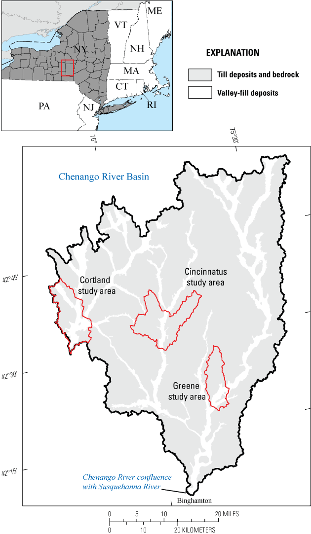
Maps showing location of study areas in the Chenango River Basin, New York.
In the Cortland study area, four water suppliers withdraw drinking water from 10 large-capacity production wells, which supply a total average daily rate of 3.6 million gallons per day (Mgal/d) from unconfined sand and gravel aquifers. Unconfined aquifers are particularly susceptible to contamination from land-surface activities because of their relatively shallow depth to the water table and the high permeability of coarse-grained deposits. Land uses in parts of this study area are urban and agriculture; these land uses store, apply, or generate pollutants that have the potential to contaminate nearby water resources. Several locations have contaminated groundwater, including from former hazardous-waste sites (Miller and others, 1998).
In the Greene and Cincinnatus study areas, one water supplier consisting of three wells in each of these rural study areas taps a confined (or semiconfined) aquifer because of the relatively thin unconfined aquifer. These are complex hydrogeologic settings in which to delineate the area contributing recharge to the wells because the semiconfining unit impedes the vertical connection with the overlying surface sources of recharge. Because of the relatively thin unconfined aquifer, options for alternative supplies are limited if there are concerns about the quality of water pumped by these wells.
Purpose and Scope
This report describes the hydrogeology of three study areas in the Chenango River Basin and documents the design and calibration of numerical groundwater-flow models for the purpose of delineating the areas contributing recharge to 16 production wells supplying drinking water. The Cortland study area includes four water suppliers: the City of Cortland and Town of Cortlandville each consist of three wells, and the Village of Homer and Village of Hamilton operate two wells each. These 10 wells are screened in a relatively shallow unconfined aquifer of well-sorted coarse-grained deposits of glacial origin. Each of the Green and Cincinnatus study areas include one water supplier, the Village of Green and Town of Cincinnatus, where each operate three wells. These six wells are screened near the top of the bedrock surface in a confined aquifer of poorly to well-sorted coarse-grained deposits of glacial origin.
The simulated areas contributing recharge to the production wells and the associated simulated groundwater traveltimes from recharging locations to withdrawal points are shown on maps for average pumping rates and average, steady-state hydrologic conditions. In the Cortland study area, an extensive groundwater-level and streamflow dataset allowed for calibration by inverse modeling using nonlinear regression to estimate the optimal set of parameter values. Summary statistics from nonlinear regression were used to evaluate the uncertainty associated with the predicted contributing area to the wells for this study area. Without an evaluation of the uncertainty associated with the model prediction, the contributing area to a well or well field may be underestimated, thereby leaving the well inadequately protected. A map depicts the results of the uncertainty analysis of the simulated area contributing recharge expressed as a probability distribution.
Overview of Study Area Settings
The Cortland, Cincinnatus, and Greene study areas lie within the Chenango River Basin, a subbasin of the Susquehanna River Basin, in central New York (fig. 1). The region’s climate is classified as warm-summer humid continental. The average annual temperature is in the mid-40s degrees Fahrenheit (°F), with average temperatures in the low 20s °F during the winter and mid-60s °F during the summer. Annual precipitation averages about 42 inches in the basin. Precipitation typically is distributed fairly uniformly throughout the year. Annual precipitation was as low as 32 inches during the early 1980s drought and was as high as 50 inches during the late 1970s wet period (Miller and others, 1998; National Oceanic and Atmospheric Administration, 2020).
The Chenango River Basin lies in the Appalachian Plateau physiographic province. Gently dipping shale and siltstone bedrock underlie the dissected plateau, which is characterized by extensive uplands separated by deeply incised, steep-walled valleys. Topographic relief in the study areas is 800 feet (ft) or more. Land-surface altitudes range from 1,080 to 1,910 ft in the Cortland study area, from 900 to 1,700 ft in the Greene study area, and from 1,000 to 1,980 ft in the Cincinnatus study area.
During multiple continental glaciations, glacial ice deeply eroded existing stream and river valleys in the study areas. The unconsolidated deposits filling the valleys and mantling the uplands are almost all from the last glaciation. In the valleys, the deposits primarily consist of three depositional facies that are locally successive but transgressive over longer distances (Randall, 2001). The three depositional facies are early deglacial, proximal, or ice-contact facies of predominantly sand, gravel, and silt varying widely in degree of sorting and deposited close to active ice and (or) amid abundant stagnant ice masses (generally referred to as “kame deposits” in this report); mid-deglacial distal facies of lacustrine silt and clay deposited in moderately large bodies of water at distance from the active glacial ice; and late-deglacial and postglacial facies of surficial sand and gravel that are well sorted and deposited as alluvium and outwash most commonly atop mid-deglacial facies (fig. 2). The uplands are mantled by till with local bedrock outcrops. The till consists of unsorted silt, clay, sand, and stones directly deposited by glacial ice as lodgment till and during deglaciation as ablation till. Thick deposits of till in the valley are referred to as till-moraine in this report.
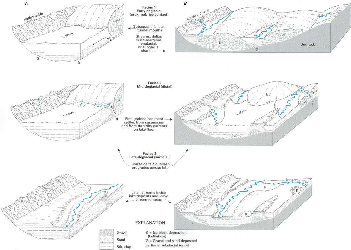
Cross sections showing idealized representation of depositional facies for two sequences. A, Active retreat sequence. B, Stagnation-zone retreat sequence in the glaciated Northeast (Randall, 2001).
Delineation of Areas Contributing Recharge to Production Wells
Many hydrologic features and processes may affect the size, shape, and location of the area contributing recharge to a well. Features and processes, such as groundwater systems with irregular geometry and complex lithology, or the interaction between individual pumping wells and hydrologic features such as surface-water bodies, are difficult to represent with analytical methods. Three-dimensional finite-difference numerical groundwater-flow models, however, can best represent these and other geologic and hydrologic features and processes.
Groundwater levels and flows were simulated in the surficial deposits and the underlying bedrock in the three study areas by using the finite-difference numerical model code MODFLOW–NWT (Niswonger and others, 2011), which is a Newton formulation for MODFLOW–2005 (Harbaugh, 2005). MODFLOW–NWT increases numerical stability and allows for unconfined simulation of thin surficial deposits of steeply sloping hills, such as the uplands bordering the valleys in the study areas. Areas at the water table that contribute water to discharge locations, such as pumping wells, are a function of long-term hydraulic gradients in the aquifer. Thus, a steady-state model that represents long-term average annual hydrologic conditions is appropriate for delineating areas contributing recharge to the production wells. Areas contributing recharge to the production wells that supply drinking water were determined on the basis of these steady-state model simulations and by use of the particle-tracking program MODPATH (Pollock, 1994). The particle-tracking program calculates groundwater-flow paths and traveltimes based on the head distribution and fluxes between model cells computed by the groundwater-flow simulation. Areas contributing recharge were delineated by forward tracking of particles from recharging areas to the discharging wells. One particle at the water table for each model cell was used. For most MODPATH simulations, particles were allowed to pass through model cells with weak sinks, which remove only a part of the water that flows into the cell (for example, a model cell simulating a weakly gaining stream). Pass-through weak-sink option was used because simulated contributing areas to a well that is a strong sink may be larger and thus more conservative in terms of land-use protection than if particles were stopped at weak sinks. All of the model input and output files developed as part of this study are provided in a separate model archive (Friesz and others, 2022).
The three study areas are in narrow glacial valley-fill settings bordered by extensive uplands in the Chenango River Basin. The Cortland study area has multiple water suppliers with wells screened in an unconfined sand and gravel aquifer. The available observation dataset (measured groundwater levels and streamflows) allowed for calibration with inverse modeling using nonlinear regression. Summary statistics from nonlinear regression were used to provide a measure of the uncertainty of the predicted contributing areas. The Greene and Cincinnatus study areas each have one water supplier with wells that tap a confined or semiconfined sand and gravel aquifer. The quantity and type of observations available in these two study areas were limited, which allowed only a rough manual (trial and error) calibration of the groundwater system.
Cortland Study Area
The Cortland study area in west-central Cortland County is primarily of the Otter Creek Basin and Factory Brook Basin, southwest–northeast trending and northwest–southeast trending valleys, respectively, that join with three valleys formed by the West and East Branch Tioughnioga Rivers and the Tioughnioga River (fig. 3). Four water suppliers, two in Otter Creek Basin (City of Cortland and Town of Cortlandville) and two in Factory Brook Basin (Village of Homer and Village of Hamilton), withdraw drinking water from 10 large-capacity wells (table 1), which supply a total of 3.6 Mgal/day from an unconfined sand and gravel aquifer primarily of glacial origin.
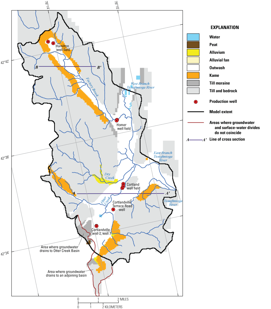
Map showing surficial geology, production wells, location of geologic sections, and model extent, Cortland study area, New York.
Table 1.
Withdrawal rates for production wells in the Cortland study area, New York.[gal/min, gallon per minute; ft3/s, cubic foot per second; --, no data]
A USGS study in Otter Creek Basin by Miller and others (1998) developed a numerical model to simulate groundwater flow in the valley-fill deposits. One of the purposes of this original model was to determine areas contributing recharge to the production wells from which drinking water is withdrawn. Uplands bordering the valley-fill deposits were incorporated indirectly into the original model by adding streamflow and groundwater discharge from these uplands at the edge of the model. Simulated areas contributing recharge to most production wells extended to this model boundary, indicating that uplands outside the model may be contributing water to the wells. Land cover in the uplands near some of the wells includes extensive agricultural land uses. If groundwater flow in the uplands was also to be simulated in a new model, the addition would help ensure that the entire area that contributes water to the production wells is included. Miller and others (1998) also provided an extensive calibration dataset at long-term average annual conditions and a detailed description of the surficial geology and associated hydraulic properties. These hydraulic property values were used for many lithologic units in this study area and for the Greene and Cincinnatus study areas. This previous groundwater model of the Otter Creek valley was calibrated to this hydrologic dataset manually to provide a reasonable match between observations and simulated groundwater levels and streamflows. Manual calibration may not provide the optimal set of parameter values that give the best fit to the observations and does not provide a means for quantitatively assessing the uncertainty in the predicted contributing areas to the wells.
Hydrogeology
The Cortland study area of 50.2 square miles (mi2) includes the Otter Creek and Factory Brook Basins along with small parts of West Branch and East Branch Tioughnioga River Basins and of Tioughnioga River Basin (fig. 3). Otter Creek and Factory Brook are tributaries to the West Branch Tioughnioga River, which in turn joins with the East Branch Tioughnioga River to form the Tioughnioga River. In the headwaters of Otter Creek Basin, groundwater and surface-water divides do not coincide (Miller and others, 1998). Groundwater in the valley-fill deposits from an adjoining basin flows northeastward toward Otter Creek Basin, whereas groundwater inflow to the valley from an adjoining upland hillslope flows away from Otter Creek Basin (fig. 3).
Glacial and postglacial deposits (fig. 3) overlie shale and siltstone bedrock in the study area. The altitude of the bedrock surface beneath these deposits is shown in figure 4; the bedrock surface rises 1,090 ft from the valleys to the highest areas in the uplands. A discontinuous layer of till deposited directly on the bedrock by glacial ice consists of an unsorted mixture of sediments ranging in size from clay to boulders.
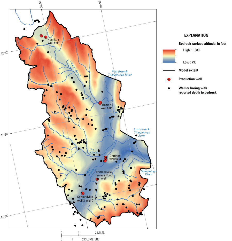
Map showing altitude of the top of the bedrock, Cortland study area, New York.
In the valleys, an unconfined aquifer consisting of mostly sand and gravel outwash generally overlies a confining unit of lacustrine very fine sand, silt, and clay deposits, which in turn overlie a confined to semiconfined aquifer of sand and gravel basal deposits of mostly ice-contact kame deposits (Miller and Brooks, 1981; Miller and others, 1998). In some areas near the valley walls, surficial kame deposits directly overlie the lower sand and gravel unit. The vertical distribution and thickness of these surficial deposits along two generalized west–east geologic sections through Otter Creek Valley and Factory Brook Valley, drawn based on the surficial mapping and geologic sections in Miller and Brooks (1981) and Miller and others (1998), are shown in figure 5. In Otter Creek valley, the unconfined sand and gravel of mostly outwash ranges from 40 to 80 ft thick. The lacustrine very fine sand, silt, and clay deposits, where present, range from about 170 ft thick in the west part to 90 ft thick in the east part of Otter Creek valley. Buried kame deposits are generally 60 to 170 ft thick in Otter Creek valley but thinner (2 to 30 ft) north of Otter Creek valley in the West Branch Tioughnioga River valley. In Factory Brook valley, the unconfined aquifer is about 100 ft thick but there was limited lithologic information to determine the thickness of the lacustrine unit and confined aquifer. A detailed description of the hydrogeology of the study area, including its glacial depositional history, is available in Miller and Brooks (1981) and Miller and others (1998). The digital hydrogeologic maps developed as part of the present study that serve as the basis for the framework of the groundwater-flow model are available as a USGS data release (Woda and others, 2022). Data sources and the methods used to develop the hydrogeologic maps are described in Finkelstein and others (2022).
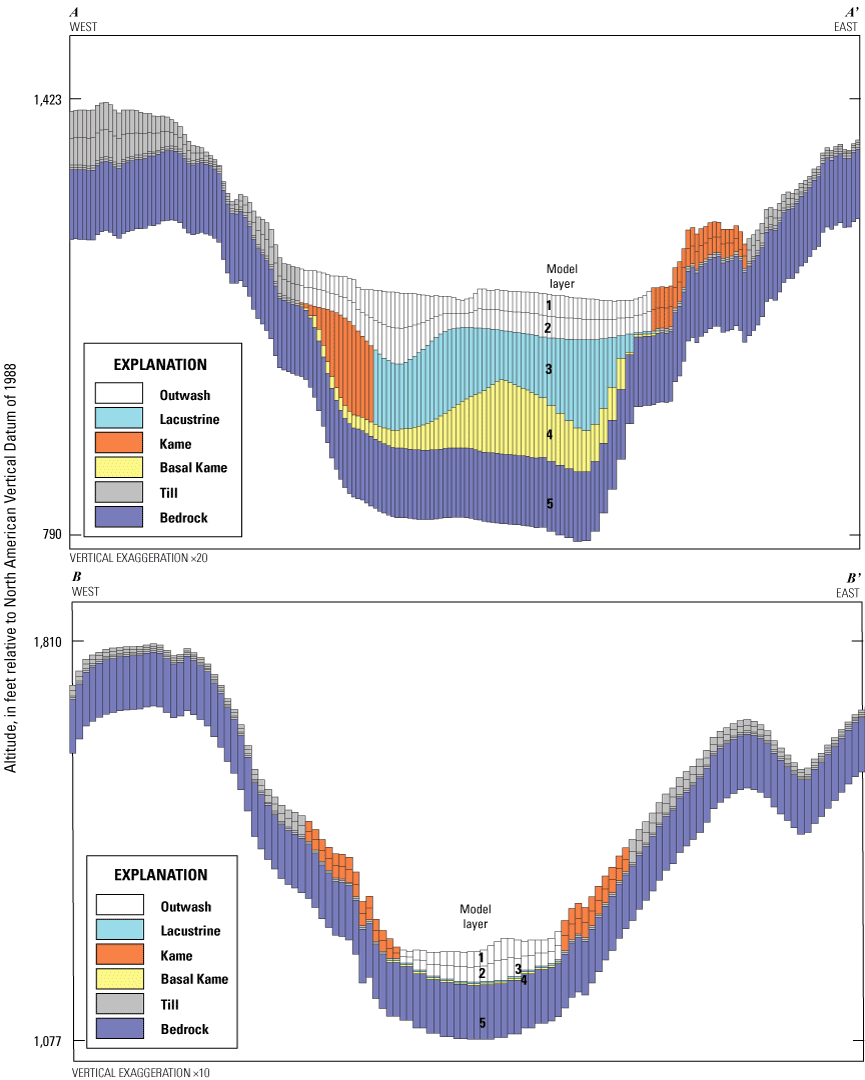
Graphs showing geologic sections and model representation (lines of sections A–A’ and B–B’ are shown in fig. 3), Cortland study area, New York.
Numerous aquifer tests have been done in Otter Creek Basin to estimate horizontal hydraulic conductivity of the principal glacial deposits (Miller and others, 1998). Aquifer-pump tests, completed in the well-sorted sand and gravel outwash deposited by meltwater typically distal to the ice front, indicated hydraulic conductivity values ranging from 880 to 1,150 feet per day (ft/d) in the western and central parts of the valley and lower values of 220 to 380 ft/d in the eastern part of the valley and adjacent to Tioughnioga River. Analysis of slugtests in mostly outwash mixed with some alluvial sediments from upland hillslope runoff near the valley wall indicated hydraulic conductivity values ranging from 3 to 140 ft/d. Hydraulic conductivity values from aquifer-pump test results in kame deposits in the unconfined and confined aquifer ranged from 60 to 85 ft/d; these ice-contact deposits can range from poorly sorted to well-sorted sand and gravel. Hydraulic conductivity values of 2 ft/d from slugtest and grainsize analyses were estimated for lacustrine deposits of very fine sand and silt that were deposited in proglacial lakes.
For postglacial deposits (alluvium and streambed deposits) and shale and siltstone bedrock, measurements of hydraulic conductivity and transmissivity have been made in other areas of the Susquehanna River Basin. Randall (1978) calculated hydraulic conductivity of alluvium described as silty gravel at seven field sites that ranged from 13 to 134 ft/d and averaged 43 ft/d. Yager (1986) estimated hydraulic conductivity of coarse-grained bed sediments of the Susquehanna River as 1 and 6 ft/d. For the shale and siltstone bedrock, Randall and Mills (2020) calculated a median transmissivity of 42 feet squared per day (ft2/d) from short-term pump tests.
Recharge in upland till and bedrock areas such as in the Cortland study area is primarily from direct infiltration of precipitation but may also include leakage from streams. Recharge rates in upland settings are conceptually highly variable, ranging from near zero in low-permeability tills on steep topography, where the water table is near land surface, to values approaching the maximum water available for recharge (precipitation minus evaporation) in high-permeability tills on moderate slopes, where the water table is perennially below the land surface.
Sources of recharge to the valley-fill aquifers include direct infiltration from precipitation, runoff from adjacent upland hillslopes, and natural infiltration from streams that cross a valley from upland areas. In some cases, pumping by wells may also induce water from the streams. In Otter Creek Basin, streams that drain the uplands lose water as they flow across the transmissive valley-fill deposits, especially near the upland-valley contact (Miller and others, 1998).
Development of Groundwater-Flow Model
Groundwater levels and flows were simulated in this valley-fill and upland setting that encompasses 50.7 mi2 in west-central Cortland County. The groundwater-flow model was calibrated based on 69 groundwater-level and streamflow (base flow) observations, most of which were measured May 28 to June 4, 1991, during average annual hydrologic conditions (Miller and others, 1998). It was assumed that long-term average annual conditions would be similar if more recent climatic conditions were also considered. Well withdrawals during this 1991 calibration period were simulated in the model and then replaced with 2010–15 average withdrawal rates to delineate the contributing areas to the production wells that supply drinking water. Most boundary conditions and hydraulic properties were represented by parameters (table 2) for calibration by nonlinear regression and for evaluating model-prediction uncertainty.
Table 2.
Definition of model parameters and statistics on parameter values, whether estimated or specified, Cortland study area.[VANI, ratio of horizontal hydraulic to vertical hydraulic conductivity; HK, horizontal hydraulic conductivity; ft/d, foot per day; --, not applicable]
Model Extent and Spatial Discretization
Groundwater flow in the unconsolidated deposits and underlying bedrock was simulated by a five-layered numerical model with a uniformly spaced finite-difference grid in the horizontal. The geographic extent of the model coincided with the physical boundaries of the flow system. Topographical divides in the relatively low-permeability till, where groundwater and surface-water divides are most likely to coincide, were used for most of the lateral extent. As mentioned in the “Hydrogeology” section for the Cortland study area, groundwater and surface-water divides do not coincide in the upper part of the Otter Creek Basin. The extent of the model in this area was along this groundwater divide and adjacent till uplands. In the transmissive valley-fill deposits and adjacent till uplands of the West Branch and East Branch Tioughnioga Rivers and the Tioughnioga River in the north and east parts of the model, the extent was distant from the production wells so that the effect of model boundaries on simulated heads near the area likely to be within the contributing area of the wells were minimized. The active model represented an area of 50.7 mi2, consisted of 529 rows and 331 columns, and included a total of 452,630 cells each with 125 ft on a side.
Vertical discretization of the five-layered model was based on lithology and surface-water features (fig. 5). The lithologic units were based on geologic and hydrologic sections in Miller and Brooks (1981) and Miller and others (1998). The surficial materials were subdivided vertically into four-model layers. In the valley-fill deposits, the top two layers (layer 1 and 2) represented mostly outwash deposits but also included kame deposits, till-moraine deposits, and postglacial alluvial deposits. This unconfined aquifer was subdivided into two layers to simulate groundwater flow near the streams accurately. Layer 3 in the valleys represented mostly lacustrine deposits and some kame deposits. Layer 4 in the valleys represented basal kame deposits. Thin till deposits in the valleys were incorporated into adjoining stratified deposits. In the uplands, till deposits were represented in all four layers. Shallow bedrock areas in the uplands less than 13 ft from the land surface were simulated as till deposits. The bottom layer (layer 5) represented bedrock with a constant thickness of 100 ft throughout the model beneath the surficial deposits. The bottom layer allows for flow in bedrock areas where surficial deposits are relatively thin, such as beneath the uplands. Ponds were simulated in layer 1 and the wells for drinking-water supply were simulated in layer 2.
Hydrologic Boundaries
Hydrologic boundaries include the movement of water into and out of the groundwater-flow model. These hydrologic boundaries include recharge from precipitation, the interaction between streams and aquifers, and well withdrawals and associated return flows.
The spatial distribution of recharge rates was applied based on the results of a soil-water-balance model. Yager and others (2018) calculated mean recharge rates for 2000–13 for the glaciated conterminous United States at a resolution of 250 by 250 meters. The soil-water-balance method uses spatially distributed variables such as climate, soil type, land use, and soil water capacity (Westenbroek and others, 2010). Mean annual recharge rates for the 2000–13 period ranged spatially from 8.9 to 28.2 inches per year (in/yr) in the Cortland study area (fig. 6). Lower rates were calculated for upland deposits with low infiltration capacity and developed land cover, and higher rates were calculated for valley-fill deposits with high infiltration capacity and undeveloped land cover. The mean annual recharge rate averaged spatially over the modeled area was 13.4 in/yr. A dimensionless parameter R_Mult (table 2) with a value of 1 multiplies the spatially varying recharge rates. This parameter was not considered for calibration by nonlinear regression; instead, the uncertainty in these recharge rates was included in the uncertainty analysis of the simulated contributing areas to the wells.
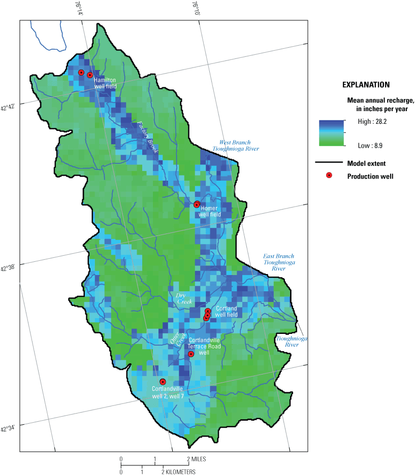
Map showing mean annual recharge rates from 2000 through 2013, Cortland study area, New York.
Stream-aquifer interactions were simulated as a head-dependent flux boundary in layer 1 (fig. 7) by using the streamflow-routing package (Niswonger and Prudic, 2005) developed for MODFLOW. The streamflow-routing package accounts for gains and losses of water in each stream cell and routes streamflow from upstream cells to downstream cells. Stream altitudes were determined from light detection and ranging (lidar) imagery (Cortland County, New York, 2017). Each streamflow-routing cell requires a conductance term that incorporates the geometry and vertical hydraulic conductivity of the streambed. Water depths and bed thicknesses of 1 ft were used to determine the top and bottom bed altitudes from surface-water altitudes. Simulated streams were assigned widths ranging from 5 to 10 ft for small tributaries, 20 ft for some stream reaches of Factory Brook and Otter Creek, 50 ft for West Branch and East Branch Tioughnioga Rivers, and 100 ft for Tioughnioga River. A parameter, SB_K (table 2), defined the vertical hydraulic conductivity of the streambed materials. Base flows entering the model from areas not directly simulated (West Branch and East Branch Tioughnioga Rivers) were specified at the first boundary stream cell. Streamflows were specified based on base-flow statistics (base-flow index; average proportion of streamflow that is base flow) from the Tioughnioga River at Cortland, New York, streamgage (station number 01509000) (USGS, 2020a). The area-weighted average of base flow from this long-term streamgage was used to calculate base flow at the West Branch and East Branch Tioughnioga Rivers based on their respective drainage area sizes. The model contained a total of 4,286 streamflow-routing cells.
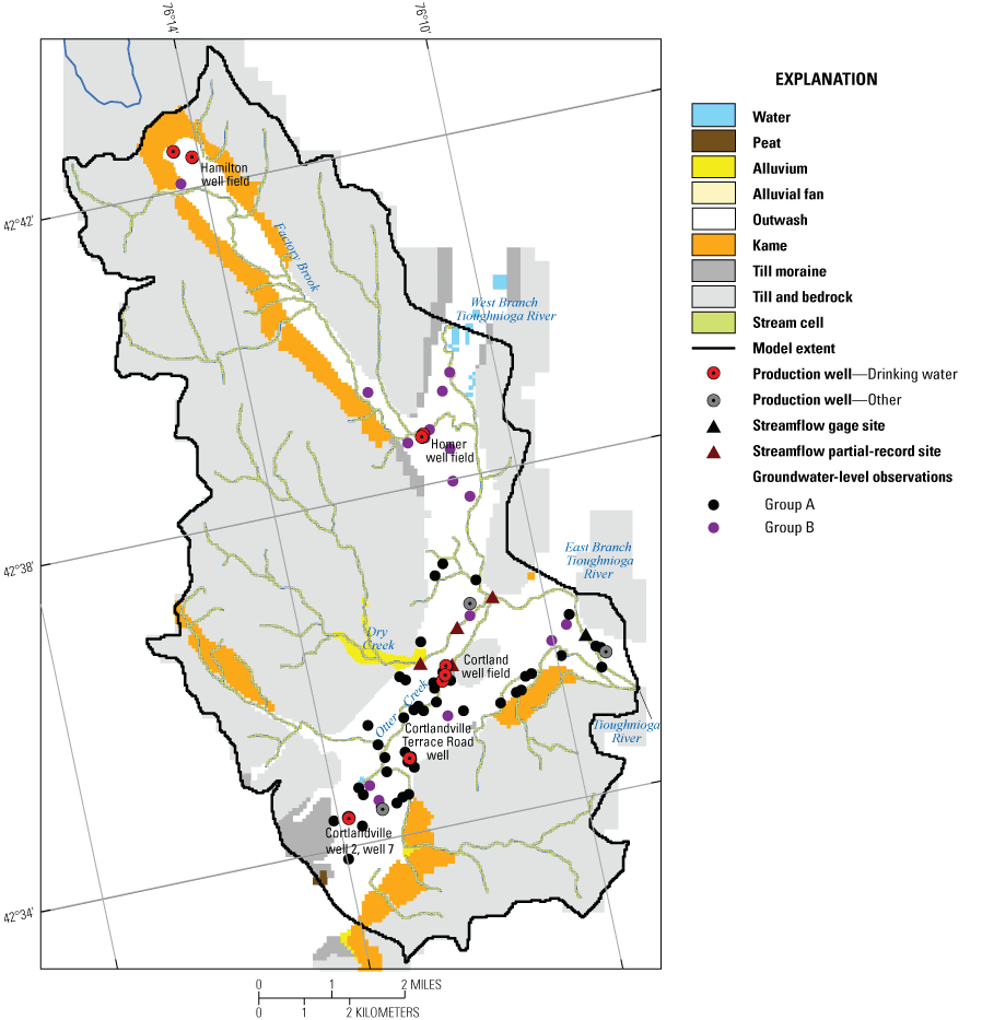
Map showing groundwater-level observations, partial-record streamgages, model stream cells, and pumping wells during 1991 calibration period, Cortland study area, New York.
Well withdrawals during the 1991 calibration period in or near the Otter Creek Basin were from six high-capacity production wells (Miller and others, 1998). For well withdrawals in other areas of the modeled area, it was assumed that 2010–15 average well withdrawals from the Village of Homer (two production wells) and Village of Hamilton (two production wells) adequately represented pumping rates from these wells during 1991. A total of 10 wells totaling 4,752 gallons per minute (gal/min), were simulated in the model during the calibration period (table 1). Withdrawals from small-capacity domestic wells were not included in the model simulations. Most pumped water from domestic wells is returned to the aquifer through nearby onsite septic systems with little net change in flow.
Water withdrawn by the City of Cortland, Town of Cortlandville, and the Village of Homer was used in sewered areas and then treated at a wastewater facility before discharging to the Tioughnioga River (City of Cortland, New York, 2020). One of the high-capacity wells was an extraction well at a hazardous waste site; after onsite treatment, all water pumped from this extraction well was returned to the aquifer through recharge basins near the well (Miller and others, 1998). Infiltration of this pumped water was simulated in 10 model cells. For the remaining wells in the City of Cortland, it was assumed that pumped water was either treated at the wastewater facility or that by not including return flow it would have negligible effects on model calibration results.
Hydraulic Parameters
Hydraulic properties of the aquifer to transmit water were defined by model parameters using zonation; these parameters were assigned on the basis of geologic units (table 2). Horizontal hydraulic conductivity of glacial stratified deposits was represented by six parameters. Lacustrine, basal, and kame deposits were each represented by one parameter (HK_Lac, HK_Basal, and HK_Kame). The final calibrated model divided the outwash into three parameters. Parameter HK_Outwash1 represented most outwash deposits in the Otter Creek Valley except in areas along the valley edges. Results of aquifer pumptests indicated high horizontal hydraulic conductivity in the western and center areas of this valley. Parameter HK_Outwash2 was assigned to the remaining outwash deposits in the Otter Creek Valley along the valley edges and the valley southward of the confluence of Factory Brook and West Branch Tioughnioga River to the Tioughnioga River where it exits the model. Parameter HK_Outwash3 represented outwash in Factory Brook Valley and in the West Branch Tioughnioga River Valley north of its confluence with Factory Brook. Available data were limited concerning hydraulic conductivity of outwash deposits in this area and few observations, but during the calibration process, it was determined that a lower value of horizontal hydraulic conductivity than the other two outwash parameters would improve the fit to the groundwater levels.
Upland till and the till-moraine deposits were each represented by one parameter (HK_Till and HK_Till-Mor). Postglacial deposits of alluvium and alluvial fan deposits were represented by parameter HK_Alluvial. Model cells containing small ponds were assigned a high hydraulic conductivity value of 2,000 ft/d to simulate the flat gradient across these features. Finally, parameter HK_Rock represented shale and siltstone bedrock.
The geologic units have various levels of local-scale interfingering of higher and lower hydraulic conductivity sediments, which can cause higher values of hydraulic conductivity in the horizontal direction compared to the vertical direction. The ratio of horizontal to vertical hydraulic conductivity (VANI) for the geologic units was each represented by one parameter (table 2).
Model Calibration
The steady-state groundwater-flow model was calibrated with the inverse modeling program UCODE–2014 (Poeter and others, 2014; Hill and Tiedeman, 2007) using nonlinear regression that minimizes the differences, or residuals, between field (observed) and simulated water levels and base flows to obtain an optimal set of parameter values. The quality of this calibration was determined by the reasonableness of the estimated parameter values and by analysis of the residuals. Some parameters might be insensitive to the available observations and therefore cannot be estimated by nonlinear regression. Values from the literature, primarily from Miller and others (1998), were used to specify parameter values that could not be estimated by nonlinear regression.
Parameter values in the groundwater-flow model were estimated using 67 groundwater-level observations and 2 base-flow observations (fig. 7). Observations were weighted to account for the difference in the type of observations and their relative effect in nonlinear regression. Observation weights are equal to the inverse of the variance (square of the standard deviation) of the measurement and model structure error. Groundwater-level observations were divided into two groups. Group A included 49 water levels measured between May 28 and June 4, 1991, at long-term average conditions (Miller and others, 1998) with surveyed measuring-point altitudes. These water levels were measured in valley-fill deposits mostly in outwash in layers 1 and 2 in and near Otter Creek Basin. Group B included 18 water levels measured between 1931 and 1991 at various hydrologic conditions (USGS, 2019) with measuring-point altitudes estimated from land-surface altitudes determined from USGS topographical contours. These water levels were also measured in valley-fill deposits mostly in outwash in layers 1 and 2 generally throughout the modeled area. The standard deviations used in model calibration ranged from 0.47 for Group A to 1 for Group B.
Base-flow measurements during the calibration period (May 28 to June 4, 1991) at four partial-record sites, two on Otter Creek and two on Dry Creek, were used for two base-flow observations. These two observations represented the net base-flow loss between the partial-record sites (1.1 ft3/s for Otter Creek and 0.8 ft3/s for Dry Creek). The accuracy of the base-flow measurement at each partial-record site was estimated to be 10 percent. The coefficient of variation (standard deviation divided by the mean) from which the observation weight was calculated was 11 percent for the base-flow observation on Otter Creek and 16 percent for the observation on Dry Creek.
Twenty-one model parameters were evaluated with parameter estimation: 10 for horizontal hydraulic conductivity (HK_Alluvial, HK_Outwash1, HK_Outwash2, HK_Outwash3, HK_Lac, HK_Basal, HK_Kame, HK_Till-Mor, HK_Till, and HK_Rock), 10 for their associated vertical anisotropy (VANI), and 1 for streambed vertical hydraulic conductivity (SB_K) (table 2). Because the recharge estimates used in the model were derived independently, they were not adjusted during calibration. Parameter sensitivities indicated the available groundwater-level and base-flow observations provided sufficient information to permit an estimate of three parameters (HK_Outwash1, HK_Outwash2, and SB_K). Most of the remaining 18 parameters were specified based on manual calibration and values in the literature (see section “Hydrogeology” for Cortland study area) (table 2). In the uplands, final values determined by manual calibration for horizontal hydraulic conductivity for upland till (HK_Till) and shale and siltstone bedrock (HK_Rock) were 3 and 0.1 ft/d, respectively, so as to simulate the water table approximately between the land surface and the bedrock surface. There were no literature values for vertical anisotropy in central New York but a ratio of 10:1 for all surficial deposits and 1:1 for bedrock were assumed to adequately represent these materials.
Optimal values for two horizontal hydraulic conductivity parameters (HK_Outwash1, HK_Outwash2) and for streambed vertical hydraulic conductivity (SB_K) that were estimated by nonlinear regression are within a plausible range of values (table 2). Values for the two outwash parameters, HK_Outwash1 (555 ft/d) and HK_Outwash2 (543 ft/d), however, are nearly the same although aquifer tests (Miller and others, 1998) indicated that HK_Outwash1 might be much greater than HK_Outwash2. Although there were no direct measurements of streambed vertical conductivity in the study area, the SB_K value of 1.7 ft/d was considered reasonable based on the average value used by Miller and others (1998) of 3.5 ft/d determined from manual calibration, by field measurements of 1 and 6 ft/d by Yager (1986) in the Susquehanna River, and because of the number of terms required to define streambed geometry.
The uncertainties of the parameter estimates, indicated by the 95-percent linear confidence intervals (table 2), are within the ranges of reasonable values reported in the literature. A comparison of the relative precision of different parameter estimates can be made using the coefficient of variation (standard deviation of the estimated value divided by the optimal value; table 2); a smaller coefficient of variance indicates a more precisely estimated value for the parameter. The coefficient of variations ranged from 0.05 to 0.20. Parameter HK_Outwash1 was the most precisely estimated, whereas parameter SB_K was the least precisely estimated.
The quality of model calibration can be determined, both numerically and graphically, by comparison of the observations and simulated equivalents. Weighted residuals should be randomly distributed and close to zero. The average weighted residual was −0.78 ft for all groundwater-level and base-flow observations, and it ranged from a minimum of –11.58 ft to a maximum of 12.07 ft. The sum of squared weighted residuals was 188 for the calibrated model.
The relation between weighted observed values and weighted simulated values is shown in figure 8A, which symbolizes the weighted head residuals by the category of their groundwater-level group. Most values plot near a line with a 1:1 slope; the correlation between them was 0.99. Weighted water-level residuals are generally randomly distributed around zero for all unweighted simulated values (fig. 8B).
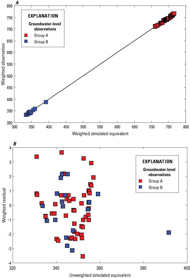
Graphs showing relation of A, weighted observation to weighted simulated equivalent and, B, weighted residual to unweighted simulated equivalent, Cortland study area, New York.
The spatial distribution of weighted base-flow and groundwater-level residuals is shown in figure 9. Unweighted residuals for groundwater levels would be one-half of the weighted residuals for Group A and the same for Group B observations (fig. 7). Weighted residuals are generally distributed randomly throughout most of the modeled area.
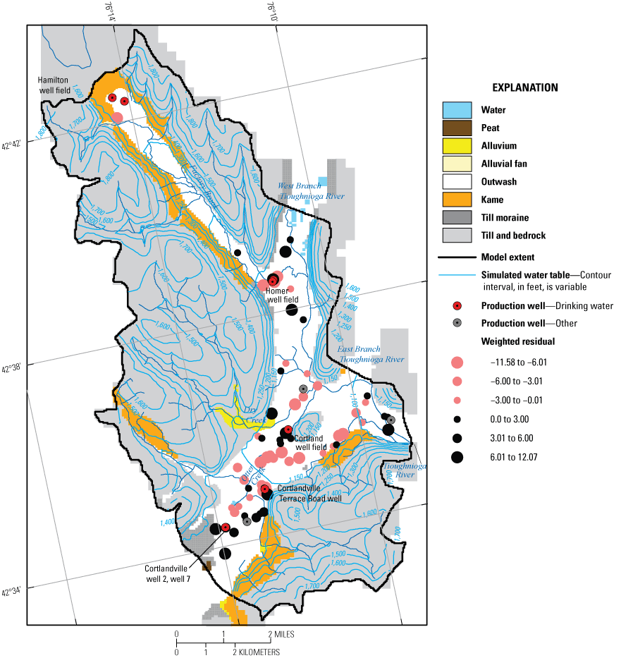
Map showing spatial distribution of weighted residuals and simulated water-table contours for calibrated, steady-state conditions, Cortland study area, New York.
The two observations of base-flow loss between partial-record sites on Otter Creek and Dry Creek compare favorably with simulated values. The values of simulated net base-flow loss for Otter Creek (1.3 ft3/s) and for Dry Creek (1.1 ft3/s) were close to observed values of 1.1 and 0.8 ft3/s, respectively.
The altitude and configuration of the simulated water table for the steady-state calibrated model are shown in figure 9 at 100-ft contour intervals except for 50-ft intervals in the valleys and near the valley-upland contacts. These simulated water-table contours are consistent with the conceptual model of groundwater flow in the study area. Groundwater generally flows from topographically high areas and discharges to streams and surface-water bodies. In the uplands, the simulated water table approximately parallels the land surface, and simulated groundwater divides generally coincide with watershed divides. The water-table gradient is steepest in the till and bedrock uplands and in valley-fill deposits near the contact and then it flattens in the more transmissive valley-fill areas of stratified deposits.
The simulated groundwater budget for the calibrated model indicated that recharge from direct precipitation provides 51.2 cubic feet per second (ft3/s), which constitutes 74 percent of the inflow. Streamflow loss accounts for the remaining inflow, 18.2 ft3/s (26 percent). Most of this streamflow loss is from tributaries downstream from the upland-valley contact, which are near areas of abrupt changes in transmissivity and near large-capacity pumping wells. Of the total inflow, 58.9 ft3/s (85 percent) of the groundwater discharges to streams, and 10.6 ft3/s (15 percent) is withdrawn by the pumping wells during the calibration period. The percentage of streamflow loss as part of the total inflow to the aquifer is within the range of groundwater model simulations in the Otter Creek Valley (32 to 38 percent) (Miller and others, 1998) and in the Tioughnioga River Valley downstream from this study (19 to 23 percent) (Miller, 2000).
Simulation results of the calibrated groundwater model indicated that the model is acceptable for use in the study to delineate steady-state areas contributing recharge to drinking-water supply wells. Model-fit statistics indicated that simulated values for groundwater levels and for base flows are generally close to observed values. Optimal parameter values are realistic, and their confidence intervals include reasonable values. The simulated water table and water budget are consistent with the conceptual understanding of valley-fill systems bordered by till uplands.
Areas Contributing Recharge and Prediction Uncertainty Analysis
Calibration of the groundwater-flow model by inverse modeling by using nonlinear regression provided an optimal set of parameter values. This optimal parameter set was estimated by minimizing the weighted residuals between the observation dataset (67 groundwater levels and 2 base flows) and simulated values. A predicted area contributing recharge to the production wells based on this optimal parameter set provides a single, most likely contributing area (deterministic contributing area) based on the current understanding of the geologic and hydrologic features of the modeled area. The parameter values, however, were estimated with different levels of uncertainty; this uncertainty in the optimal values was based on the information that the observation dataset provided on the parameters. Parameter uncertainty and its associated effects on model predictions (spatial variability of the simulated contributing area to a well) can be evaluated by a stochastic Monte Carlo analysis. The parameter variance-covariance matrix from nonlinear regression can be used to create plausible parameter sets for the Monte Carlo analysis (Starn and others, 2010). The parameter variance-covariance matrix incorporates the uncertainty of the parameter estimates and the correlation among parameters from the calibrated model. The Monte Carlo analysis was done by replacing the parameter set in the calibrated model by a plausible parameter set multiple times. The probability of a location being in the contributing area to a production well was calculated from these multiple model simulations.
Areas contributing recharge were determined for the 10 production wells that supply drinking water based on their 2010–15 average withdrawal rates (table 1). The two Village of Hamilton wells had very low average withdrawal rates (3 and 5 gal/min). At this low withdrawal rate only a small part of the water that flows into the model cell with the well screen is removed by the production well (weak sink). Because it cannot be determined whether water that enters this cell is withdrawn or continues through the groundwater system, simulations of particles for these two wells were stopped at these two weak sinks (instead of allowed to pass through weak sinks). Thus, the contributing areas to these two wells are larger, or more conservative, than if it was not a weak sink cell. In addition, the Village of Hamilton wells were not incorporated into the uncertainty analysis of the contributing areas because of their low pumping rates and the fact the simulated contributing areas to these wells were considered conservative.
Areas Contributing Recharge
Simulated deterministic areas contributing recharge and simulated groundwater traveltimes to the production wells were determined on the basis of the calibrated steady-state model for simulated pumping conditions and tracking of pathlines with the MODPATH particle-tracking program. Simulated areas contributing recharge for the 2010–15 average withdrawal rates extend upgradient from the wells to groundwater divides and topographical divides, some of which serve as model boundaries (fig. 10). Most areas contributing recharge extend beneath and beyond streams and include upland till deposits. Areas contributing recharge include isolated areas remote from the wells including small areas the size of a model cell. In addition, most wells are not overlain by their contributing area, including Cortlandville well 2 and well 7, which are overlain by the contributing area to the downgradient Cortland well field. The wells in the study area are screened in the deep part of the outwash deposits (layer 2), and recharge near the wells travels along flow paths above and around the screened interval of the well.
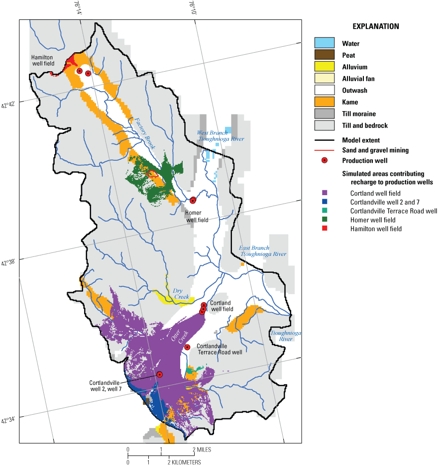
Map showing simulated areas contributing recharge to the production wells at their average pumping rates from 2010 to 2015, Cortland study area, New York.
The size of the simulated areas contributing recharge to the Cortland and Cortlandville wells in Otter Creek Basin covered a total area of 5.86 mi2. For the large total pumping rates for these wells, the contributing areas covered most of the valley southwest of the Cortland well field where there is substantial amount of urban and agriculture land uses (National Land Cover Database, 2016). Land cover in the contributing area to the Cortland well field and to Cortlandville Terrace Road well have urban land use considered high density. In the uplands, the land cover in the contributing areas to these wells is primarily agriculture and forested. The size of the contributing area to Cortlandville Terrace Road well is relatively small for its pumping rate; this well, which is situated downgradient of a long losing reach of Otter Creek that parallels the valley-upland contact, captures a substantial amount of this streamflow loss. The contributing areas to Cortlandville well 2 and well 7 are in the least developed part of the valley but include some agriculture and urban land uses. A nearby sand and gravel mining operation southeast of Cortlandville well 2 and well 7 is within the simulated contributing area to the Cortland well field.
In Factory Brook Basin, the size of the simulated areas contributing recharge to the Homer well field covered a total area of 0.99 mi2. This well field, which is screened in the deep part of the outwash deposits, is on the west edge of the Village of Homer but the land cover in its contributing area, which is distal to the well field, is primarily agriculture and forested (National Land Cover Database, 2016). However, small parts of a sand and gravel mining operation, shown in World Imagery (2018) along the southwest side of Factory Brook valley, were in simulated parts of the contributing area to the well field (fig. 10). Recharging water between the well field and its contributing area travels along shallow and intermediate depth flow paths before discharging to streams. The size of the simulated contributing area to the Hamilton wells covered 0.08 mi2. Land cover in this contributing area is agriculture and forested.
Simulated traveltime estimates from recharging locations to the production wells for the 2010–15 pumping rates are shown in figure 11. Porosity values (table 2) were specified in the model for MODPATH, but they affect only groundwater velocity and do not change the contributing areas to the wells in a steady-state simulation. Glacial deposits and postglacial deposits were assigned a porosity of 0.35 based on values determined for similar deposits in Rhode Island (Allen and others, 1963), Massachusetts (Garabedian and others, 1991), and southern New England (Melvin and others, 1992). For bedrock, a porosity of 0.05 was assigned based on values for shale bedrock (Freeze and Cherry, 1979).
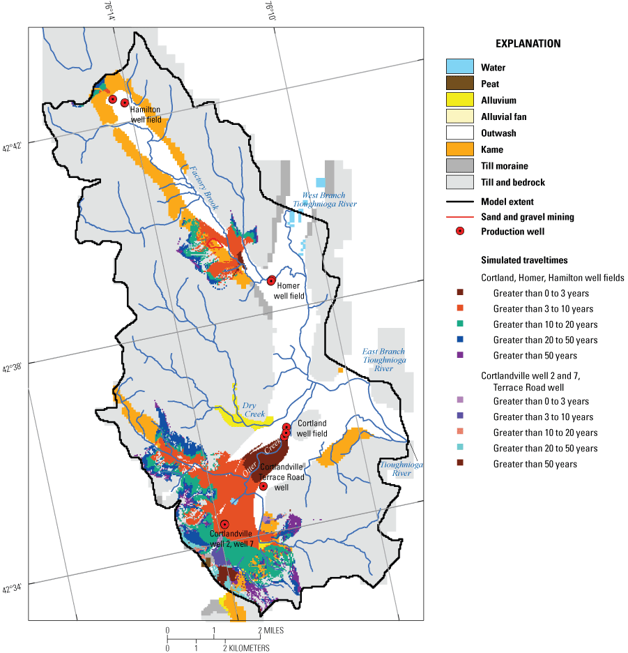
Map showing simulated groundwater traveltimes to the production wells at their average pumping rates from 2010 to 2015, Cortland study area, New York.
Traveltimes generally depend on where recharge enters the aquifer in relation to the production wells. Water that recharges the aquifer near the wells has the shortest traveltimes and youngest water, whereas water originating in the till uplands has the longest traveltimes and the oldest water. Traveltimes ranged from less than 1 year to more than 300 years; 50 percent of the traveltimes were 10 years or less. The median traveltime was 10.2 years for the wells in Otter Creek Basin and 8.7 years for the Homer well field. For the Hamilton well field, which has very low pumpage and weak sinks, the median traveltime was 20.5 years. This percentage for traveltimes 10 years or less and the relatively short median traveltimes indicate that the wells are vulnerable to contamination from activities on the land surface.
Probabilistic Areas Contributing Recharge
The effects of parameter uncertainty on model predictions (the predicted contributing area) were quantitatively measured by a Monte Carlo analysis. A Monte Carlo analysis was used to obtain the probability of a recharge location being in the contributing area of the well fields. The probability distribution is related to the information that the observation dataset provided on the estimated parameters, to prior information on specified parameters, and to the sensitivity of the simulated contributing area to the parameters. Hundreds of parameter sets generated from summary statistics of the calibrated steady-state model were used to run hundreds of model simulations in the Monte Carlo analysis. Because combinations of reasonable parameter values might result in unrealistic groundwater levels and streamflows, the parameter sets were evaluated using the pumping rates and associated observation dataset from the calibrated model. Those parameter sets that simulated realistic results were then used in Monte Carlo analysis for the 2010–15 average pumping rate scenario.
Parameter values for the Monte Carlo analysis were created from the parameter values in the model and its parameter variance-covariance matrix (Starn and others, 2010; Starn and Bagtzoglou, 2012). Parameter values that could not be estimated by nonlinear regression and thus were not included in the parameter variance-covariance matrix of the calibrated model might still be important for model predictions (for this study, the size, shape, and location of the area contributing recharge to the production wells). Horizontal hydraulic conductivity parameters of the principal glacial deposits (HK_Outwash3, HK_Lac, HK_Basal, HK_Kame, and HK_Till) were incorporated into the parameter variance-covariance matrix using their specified parameter values. Recharge rates, although calculated independently from the model, were also included in the parameter variance-covariance matrix because of the importance of this boundary condition on the simulated contributing areas to the wells. Vertical anisotropy of the surficial sediments and bedrock was not included in this analysis because they have little to no effect on the simulated contributing area to a well in a valley-fill setting for a plausible range of values (Friesz, 2010). Incorporating these five horizontal hydraulic parameters and one recharge parameter into the parameter variance-covariance matrix, however, caused large unrealistic uncertainties around the specified parameter values because the information the observations provided was insufficient. Prior information on these parameters was used to constrain this uncertainty to include most plausible values (table 2). Parameter uncertainties are from the observation dataset, but also from prior information on parameters that the modeler provided.
For the Monte Carlo analysis, the model was first run with 500 parameter sets and with the 1991 pumping rates used in calibrating the model. The nine hydraulic and recharge parameter values in each dataset replaced the corresponding parameter values in the calibrated model. Three criteria for accepting a given parameter set were used: (1) the model converged, (2) the model mass balance was 1 percent or less, and (3) a model-fit statistic (calculated error variance, which is the sum of squared weighted residuals divided by the difference between the number of observations and the number of parameters estimated by nonlinear regression) was less than a specified value. The third acceptance criterion was used so that model-prediction uncertainty would not be overestimated by using a parameter set that produced unrealistic groundwater levels or streamflows compared with that for the calibrated model. The value used for this criterion, however, can be model dependent and subjective. For this model application of the Monte Carlo analysis, a calculated error variance of 7 was selected for the third criterion, or about 2.5 times the calculated error variance of the calibrated model. Of the 500 parameter sets run with MODFLOW, 470 sets (94 percent) fit these three criteria.
A Monte Carlo analysis was then done using the parameter sets that fit the acceptance criteria for the 1991 average withdrawal rates but using the 2010–15 average withdrawal rates. The criteria for the Monte Carlo analysis that used the 470 parameter sets and these pumping rates were that the water budget error be 1 percent or less for models that converged. For the average withdrawal rates from 2010 to 2015, 467 parameter sets (99 percent) fit these criteria and thus were run with the particle-tracking program. The probability that a recharge location would be in the area contributing recharge to the production wells was determined by dividing the number of times a particle at a given location was captured by a well by the total number of accepted particle-tracking simulations; this probability was expressed as a percentage.
The probabilistic areas contributing recharge to the production wells in Otter Creek Basin and for the Homer well field for the average pumping rates from 2010 to 2015 are shown in figure 12. For this analysis, the probabilistic distribution for the closely spaced Cortland and Cortlandville well fields in Otter Creek Basin was done for the wells together. Probabilistic contributing areas to individual well fields or wells might overlap, even though the deterministic contributing areas do not overlap under a steady-state simulation. The total size of the probabilistic contributing area for the Otter Creek Basin wells and for the Homer wells was larger than the deterministic contributing areas because of the effects of parameter uncertainty. The probabilistic contributing area analysis indicated that some areas not in the deterministic contributing area, including additional areas of urban and agricultural land use, might actually be in the contributing area.
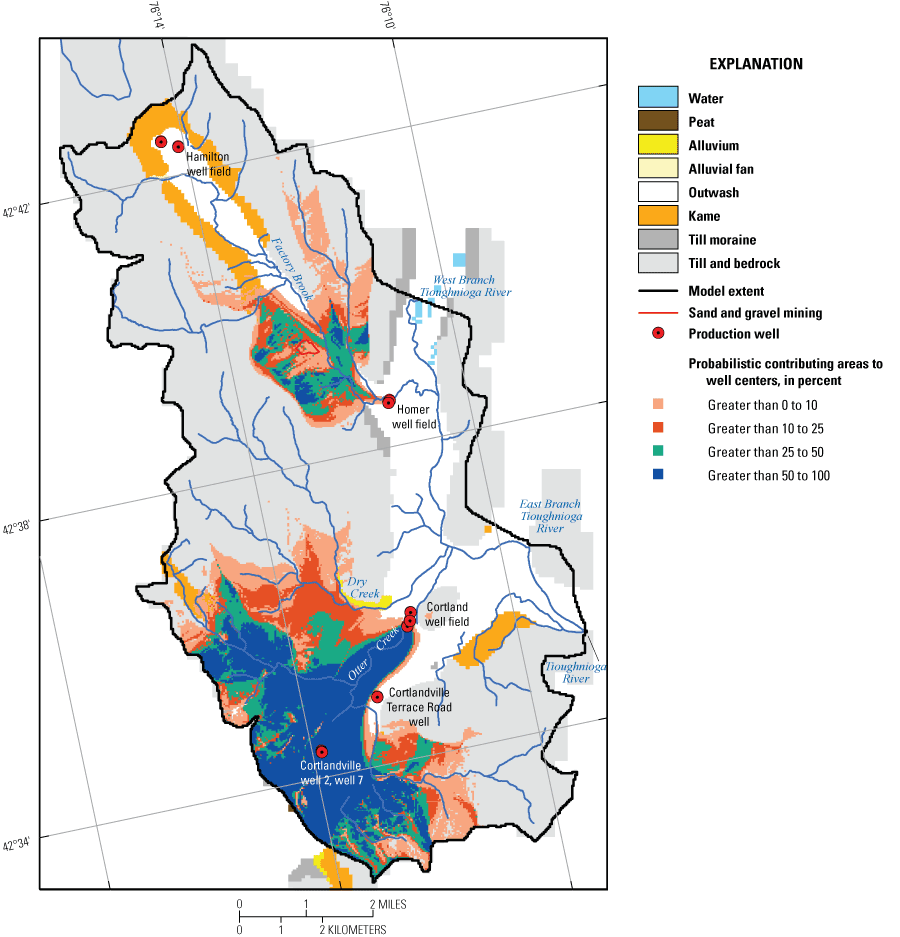
Map showing simulated probabilistic areas contributing recharge to production wells in the Otter Creek Basin and to Homer production wells, Cortland study area, New York.
In Otter Creek Basin, in most cases, areas with high probabilities (greater than 50 percent) generally coincide with the deterministic contributing areas for the Cortland and Cortlandville wells. The probabilistic contributing areas to the wells indicate additional areas in the valley and uplands might be the contributing area. Dry Creek Basin, an adjoining basin, which was not in the deterministic contributing area, might have areas that are in the contributing area to the wells. Low probabilities are generally in areas distant from the pumping wells and in areas where simulated streams intercepted precipitation recharge in the deterministic model. Additional areas that might be in the contributing area include recharge originating near the pumping wells that have relatively short groundwater-flow paths and traveltimes. In some cases, small isolated areas remote from the pumping wells that are in the deterministic contributing area are associated with low probabilities.
For the Homer well field, areas with probabilities of greater than 25 percent generally coincide with the deterministic contributing area. The probabilistic contributing area to this well field has a large spread in low probabilities, in part because in this area of the model most parameters could not be estimated by nonlinear regression. Instead these parameters were added to the uncertainty analysis with prior information, which included most plausible values. Streamflow measurements and additional groundwater levels in Factory Brook Basin might help reduce the uncertainty in the simulated contributing area to the well field by increasing the number of parameters that could be estimated by nonlinear regression. The probabilistic contributing areas indicated that precipitation recharge that discharges to Factory Brook and its tributaries in the deterministic model might instead go directly to the well field. These areas include probabilities of greater than 25 to 50 percent between the wells and the deterministic contributing area with relatively short groundwater-flow paths and traveltimes. That part of the sand and gravel mining operation along the southwest side of Factory Brook valley that is not in the deterministic contributing area is in the probabilistic contributing area associated with low probabilities of 10 percent or less (fig. 12).
Greene Study Area
The water supply for the Village of Greene, Chenango County, consists of three wells adjacent to and east of the Chenango River in a northeast–southwest trending valley-fill setting bordered by extensive upland till and bedrock (fig. 13). The three wells, which supplied an average annual rate of 169 gal/min for the 2010–15 period (table 3) to about 2,000 residents, are screened about 160 ft deep in a confined (or semiconfined) aquifer. The confined aquifer, consisting of mostly sand and gravel deposits (ice-contact kame deposits), is the most widely used aquifer in this study area because of the relatively thin unconfined aquifer (Hetcher-Aquila and Miller, 2005).
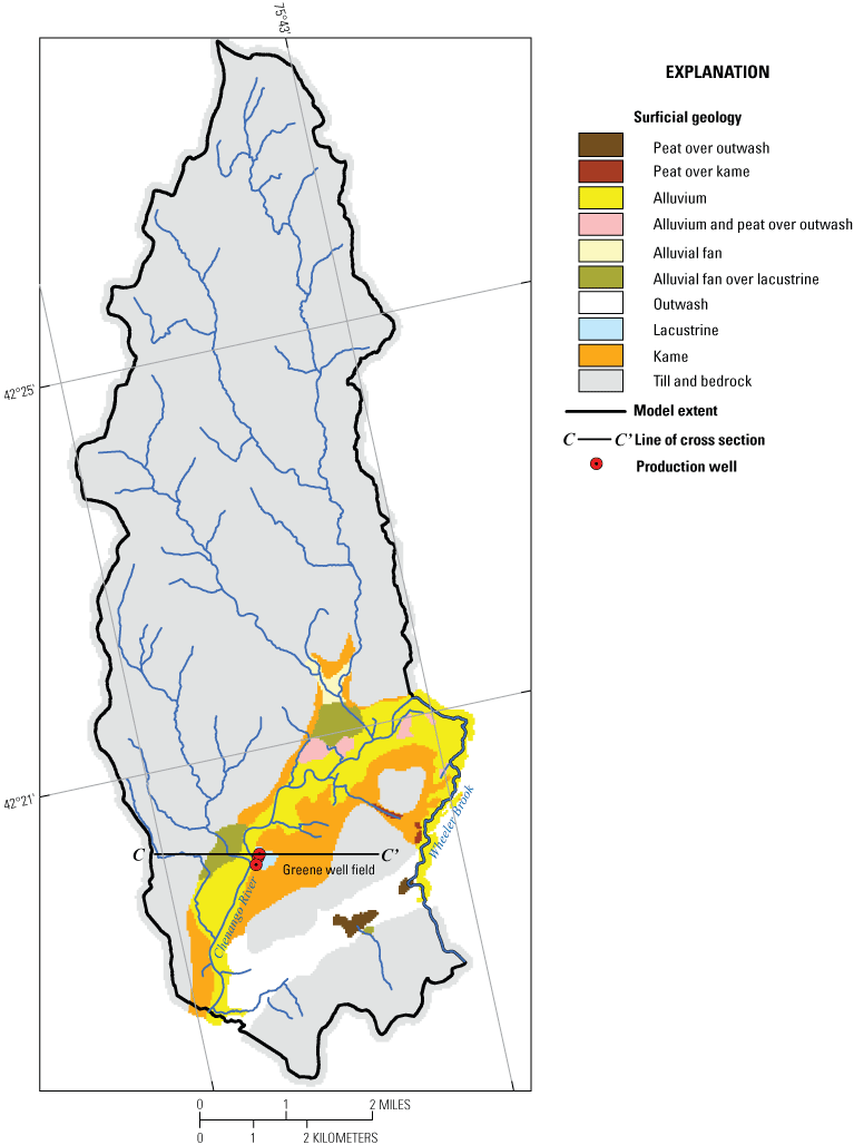
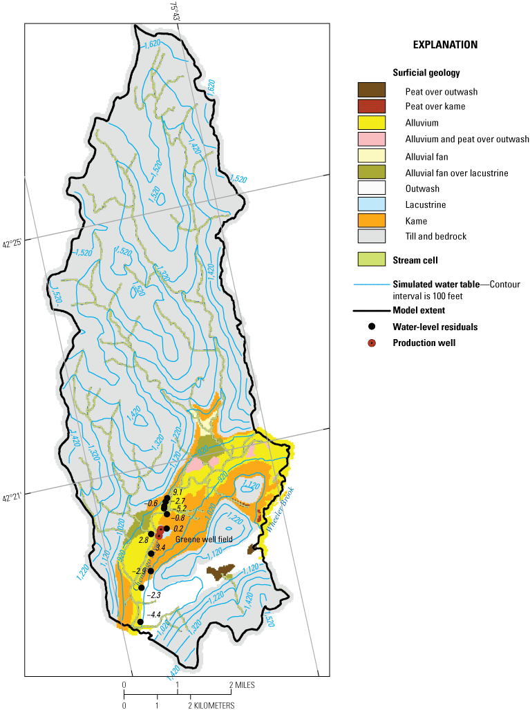
Map showing surficial geology, production wells, location of cross section, and model extent, Greene study area, New York.
Table 3.
Average withdrawal rates for production wells in the Greene and Cincinnatus study areas, New York.[gal/min, gallon per minute; ft3/s, cubic foot per second]
Hydrogeology
The Chenango River drains a northeast–southwest trending valley-fill system before it eventually joins the Susquehanna River. The surface of the shale and siltstone bedrock rises steeply from the valley by as much as 980 ft to the topographical divide in the uplands that defines the study area extent in the north (fig. 14). Glacial till mantles the shale and siltstone bedrock surface in most places except in central areas of the valleys but can range from several feet to tens of feet in the uplands (Hetcher-Aquila and Miller, 2005).
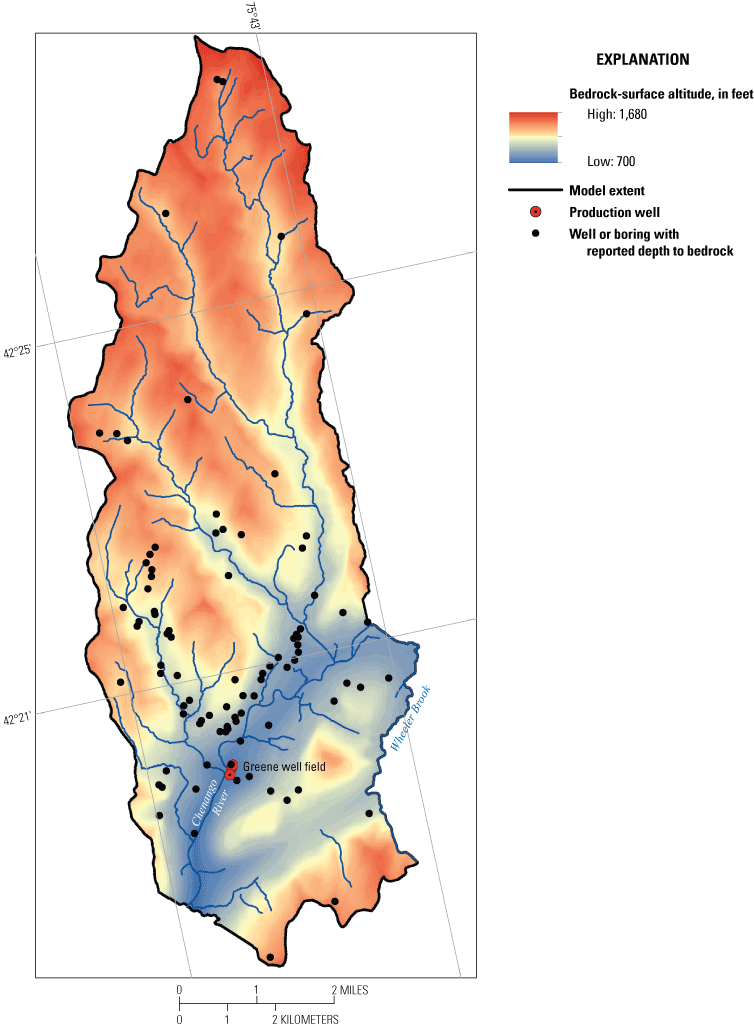
Map showing altitude of the top of bedrock, Greene study area, New York.
In the valleys, glacial deposits (outwash and ice contact of mostly kame deposits) and postglacial deposits (mostly alluvium) form an unconfined sand and gravel aquifer (Hetcher-Aquila and Miller, 2005) (fig. 13). Beneath this unconfined aquifer, along most of the northwest side of the main Chenango River valley and in central areas parallel to the main valley axis, lacustrine deposits of very fine sand, silt, and clay overlie a confined aquifer of ice-contact deposits that are poorly to well-sorted sand and gravel. The three production wells that supply potable water are screened in this confined aquifer in the center of the valley. The vertical distribution and thickness of the unconsolidated deposits, along a generalized west–east geologic section through Chenango River valley near the production wells and drawn based on the surficial mapping and geologic sections in Hetcher-Aquila and Miller (2005), are shown in figure 15. Along the southeast side of the main valley, the unconfined aquifer consists of ice-contact kame deposits extending vertically to the bedrock surface and these deposits are connected to the confined aquifer. The unconfined aquifer is generally less than 20 ft thick along the northwest and central areas of the main valley but thicker along the southeast side of the valley where kame deposits overlie bedrock. The lacustrine confining unit is as much as 160 ft thick. The confined aquifer is generally 10 to 30 ft thick in the central parts of the valley but along the northwest side of the valley buried ice-contact deposits are less than 10 ft thick or not present. A detailed description of the hydrogeology of the study area, including its glacial depositional history, is available in Hetcher-Aquila and Miller (2005). The digital hydrogeologic maps developed as part of the present study that serve as the basis for the framework of the groundwater-flow model are available from Woda and others (2022). Data sources and the methods used to develop the hydrogeologic maps are described in Finkelstein and others (2022).
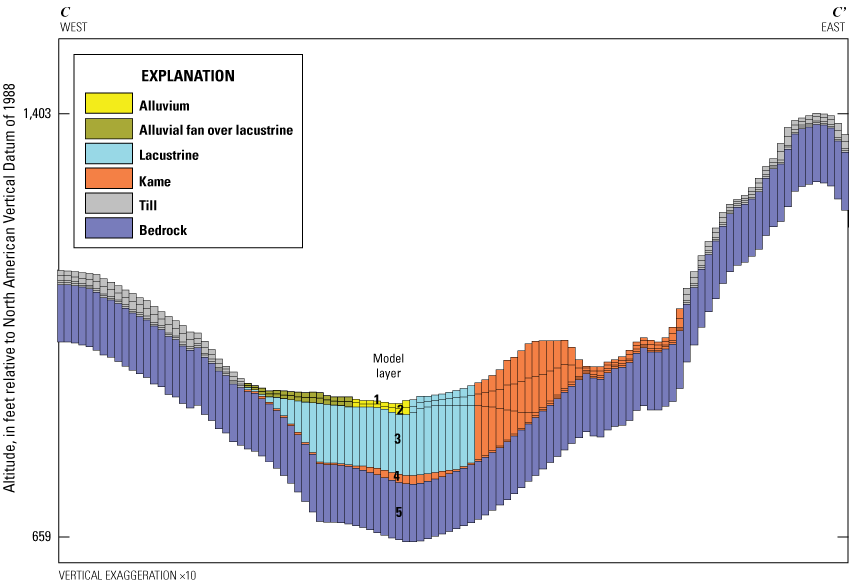
Graph showing geologic section and model representation (line of section C–C’ is shown in fig. 13), Greene study area, New York.
Sources of water to the confined or semiconfined aquifer, and thus the production wells, are an important factor in the location of their contributing areas. The fine-grained lacustrine deposits impede vertical flow to the confined aquifer from surface sources such as direct infiltration of precipitation and streamflow loss. Under pumping conditions, the increased vertical hydraulic gradient between the unconfined and confined aquifers may increase leakage through the confining unit, especially in areas of thin lacustrine deposits. Recharge to the unconfined kame deposits east of the wells likely is an important source of water because these deposits are connected to the confined aquifer. Westward and northwestward of the wells, thin ice-contact deposits may extend up along the valley wall to the land surface where recharge can also enter the confined aquifer. Another source of water to the confined aquifer may be groundwater inflow from adjacent uplands through till and shallow bedrock.
Development of Groundwater-Flow Model
Groundwater flow in the unconsolidated deposits and the underlying shale and siltstone bedrock was simulated by a five-layer model with a uniformly spaced grid. The groundwater-flow model was manually calibrated to 11 groundwater-level altitudes and to a generally shallow water table that approximates the land-surface configuration in the till and bedrock uplands. The 11 groundwater levels were measured from 1959 to 1992 at various hydrologic conditions (Hetcher-Aquila and Miller, 2005). Five of these measurements were from wells screened in the unconfined aquifer and the remaining six measurements from wells screened in the deep part of the valley in the confined aquifer. The altitudes of the measuring points were based on the altitude of the land surface determined from lidar imagery (Terrapoint USA, 2008). Because of the limited quantity of available groundwater levels and no streamflow measurements, model calibration was considered a rough estimate of hydraulic properties. Model characteristics, including hydraulic properties and recharge rates, are summarized in table 4.
Table 4.
Summary of simulated values for hydraulic properties and recharge rates in the groundwater-flow models for the Greene and Cincinnatus study areas, New York.The groundwater-flow model extended to natural hydrologic boundaries beyond the likely areas contributing recharge to the production wells. This extent also minimizes the effects of boundaries on simulated heads near groundwater divides separating Chenango River from Wheeler Brook east of the production wells. The lateral model boundaries included Wheeler Brook on the east; elsewhere, the edge of the model extended to presumed groundwater divides in the low permeable till uplands in most areas. The active model grid represented an area of 32.8 mi2, consisted of 505 rows and 192 columns, and included a total of 292,340 cells each with 125 ft on a side.
Vertical discretization of the five-layered model was based on lithology (fig. 15) from hydrogeologic mapping by Hetcher-Aquila and Miller (2005) and updated by Woda and others (2022). The unconsolidated sediments were subdivided vertically into four model layers. In the valley-fill deposits the top two layers (layers 1 and 2) represented the unconfined aquifer, which consisted mostly of alluvium, outwash, and kame deposits. Layer 3 in the valleys represented lacustrine and kame deposits. Layer 4 in the valleys represented the confined aquifer, which consists of kame deposits. The three production wells were simulated in layer 4. In the uplands, till deposits were represented in all four layers; shallow bedrock areas less than 13 ft from the land surface were simulated as till deposits. The bottom layer (layer 5) represented bedrock with a constant thickness of 100 ft.
The model of the Greene study area specified the same types of boundary conditions that the Cortland study area did to represent sources of recharge and areas of discharge. Recharge rates were applied based on the results of a soil-water-balance model (Yager and others, 2018). Mean annual recharge rates calculated by the soil-water-balance model for 2000–13 ranged spatially from 8.3 to 28.0 in/yr in the Greene study area (fig. 16). Lower recharge rates were calculated for upland till deposits with low infiltration capacity and higher rates were calculated for valley-fill deposits with high infiltration capacity. The mean annual recharge rate, averaged spatially over the modeled area, was 11.7 in/yr.
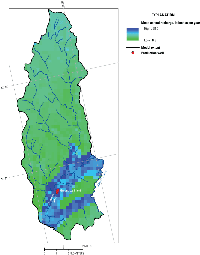
Map showing mean annual recharge rates from 2000 through 2013, Greene study area, New York.
Interactions between surface water and groundwater were simulated as a head-dependent flux boundary in layer 1 (fig. 17) by using the streamflow-routing package (Niswonger and Prudic, 2005). Stream altitudes were determined from lidar imagery. Water depths and bed thicknesses of 1 ft were used to determine the top and bottom bed altitudes from surface-water altitudes. Simulated streams were assigned widths ranging from 10 ft for small tributaries to as much as 30 ft for tributaries to Chenango River where they cross the valley, and 150 ft for the Chenango River itself. A vertical hydraulic conductivity of 3 ft/d was used to represent bed sediments. Base flow entering the model from areas not directly simulated was specified at the first boundary stream cell. Streamflows were specified based on base-flow statistics (base-flow index) at the Chenango River at Greene, New York, streamgage (station number 01507000) (USGS, 2020b). The model contained a total of 3,470 stream cells.
Map showing model stream cells, spatial distribution of water-level residuals, and simulated water-table contours for calibrated, steady-state conditions, Greene study area, New York.
Average annual withdrawal rates for 2010–15 from the three Village of Greene wells (table 3), a total of 169 gal/min, were used to represent long-term average rates. The three production wells are screened in kame deposits of the confined aquifer. Withdrawals from small-capacity domestic wells were not included in the model simulation because most of the pumped water is returned to the aquifer through nearby onsite septic systems. Water withdrawn by the production wells is used in sewered areas and then treated at a wastewater facility before discharging to the Chenango River (Town and Village of Greene, New York, 2020).
Horizontal hydraulic conductivity values were assigned on the basis of lithology (table 4). For the valley-fill deposits, final values ranged from 2 ft/d for lacustrine deposits to 200 ft/d for the outwash deposits. Till deposits ranged from 0.5 to 4 ft/d. The ratio of horizontal to vertical hydraulic conductivity was 10 for all surficial deposits and 1 for bedrock.
The altitude and configuration of the simulated water table for long-term, steady-state conditions are shown in figure 17 along with the water level residuals from the limited calibration dataset. The simulated water-table contours and flow directions are consistent with the conceptual model of groundwater flow in the study area. Groundwater flows from topographically high areas and discharges to streams. In the uplands, the water table generally parallels the land surface, and simulated groundwater divides generally coincide with watershed divides. The hydraulic gradient is steepest beneath the upland till and valley-fill deposits near the contact and flattens in the more transmissive valley-fill areas. Simulated groundwater flow in the valley-fill deposits is nearly perpendicular to the main valley stream, Chenango River, and nearly parallel to the small tributary streams that drain the uplands and become minimally gaining or losing as they flow over more transmissive valley-fill deposits. The average residual was −0.3 ft and it ranged from a minimum of −5.2 ft to a maximum of 9.1 ft.
The simulated long-term, steady-state groundwater budget for the modeled area indicated that precipitation recharge accounts for most of the total inflow (28.3 ft3/s or 83.7 percent). Streamflow loss accounts for the remaining inflow (5.5 ft3/s or 16.3 percent). Of the total inflow, 33.4 ft3/s (98.8 percent) of the groundwater discharges to streams and the remainder, 0.4 ft3/s (1.2 percent), is withdrawn by the production wells.
Areas Contributing Recharge
Areas contributing recharge and groundwater traveltimes to the Village of Greene production wells were determined on the basis of the steady-state model for simulated pumping conditions and tracking of pathlines with the MODPATH particle-tracking program. The area contributing recharge to the production wells for the 2010–15 average pumping rates (total of 169 gal/min; table 3) covers 0.35 mi2 and includes recharge originating on both sides of the Chenango River (fig. 18). The contributing area extends southeastward from the wells to the simulated groundwater divide in the uplands. The contributing area also includes isolated areas remote from the well from recharge originating on the opposite side of the river from the wells in the till uplands and near the valley-upland contact. Land cover in the contributing area to the wells is mostly agriculture and forested with some urban land uses near the valley-upland contact on both sides of the river (National Land Cover Database, 2016). On the east side of the river this urban land use is considered low density whereas on the west side of the river, this urban land use is low to high density.
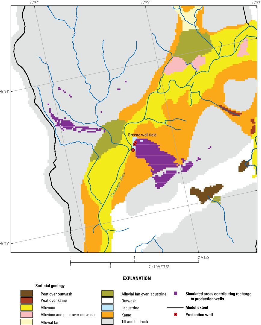
Map showing simulated areas contributing recharge to the production wells at their average pumping rates from 2010 to 2015, Greene study area, New York.
Simulated traveltime estimates from recharge locations to the production wells, based on a porosity of 0.35 for the surficial deposits and 0.05 for bedrock, are shown in figure 19. Traveltimes ranged from 3 years to more than 300 years; 9 percent of the traveltimes were 10 years or less. The median traveltime to the wells screened in this relatively deep, confined aquifer was 17.9 years. In addition to the distance from recharge location to the wells, other factors that might affect traveltimes include pumping rates, recharge rates, hydraulic conductivity, and porosity. For example, east of and near the Village of Greene well 1 and well 2, there is a traveltime interval of 20 to 50 years. Groundwater-flow paths from recharge in this interval travel to the wells partly through the low hydraulic conductivity lacustrine deposits. On the opposite side of the river from the wells and near the valley-upland contact, traveltime intervals of 3 to 10 years are adjacent to an interval of greater than 50 years that includes traveltimes of 150 to 170 years. Particle tracks show that recharge originating in the lower traveltime interval mostly travels through the confined kame deposits, whereas recharge originating in the higher traveltime interval travels through the lacustrine and the buried kame deposits.
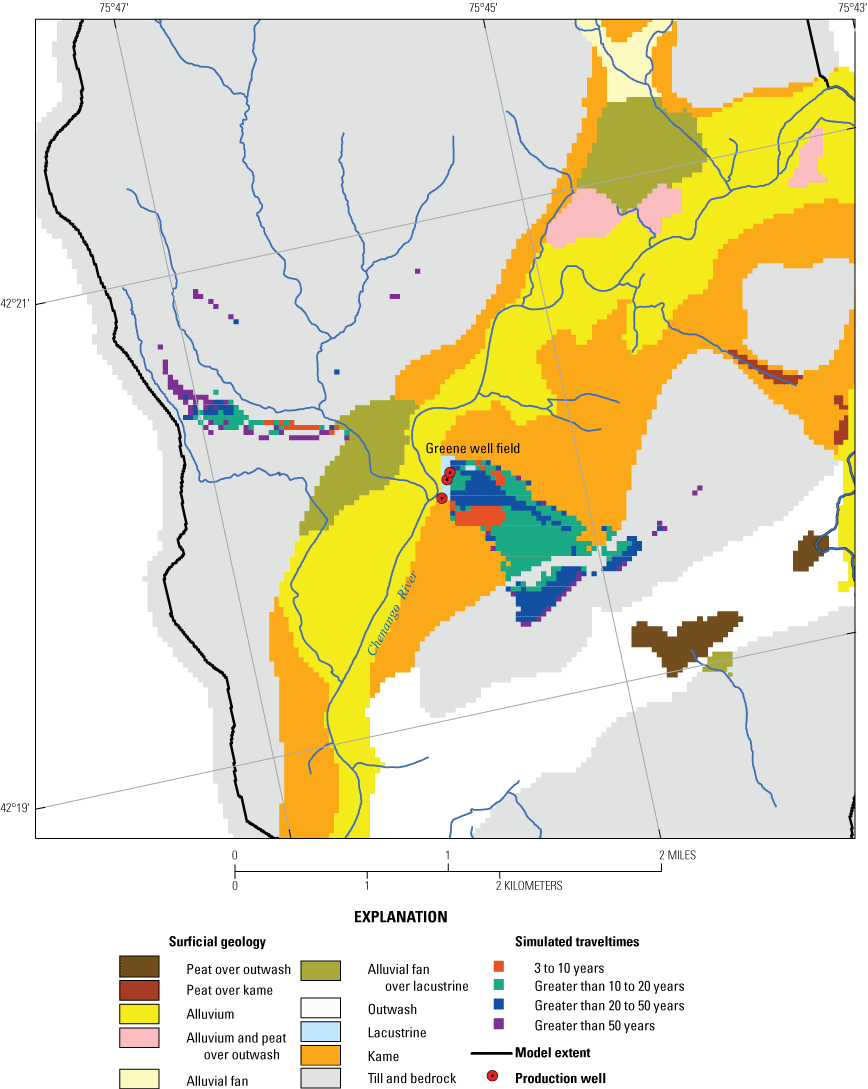
Map showing simulated groundwater traveltimes to the production wells at their average pumping rates from 2010 to 2015, Greene study area, New York.
Cincinnatus Study Area
The Town of Cincinnatus in east-central Cortland County is in a north–south trending valley-fill setting along the Otselic River, a tributary to the Tioughnioga River (fig. 20). The town’s water supply consists of two wells west of the river and one east of the river; these three wells supply an average annual rate of 34 gal/min for the 2010–15 period (table 3) to about 900 residents in this rural study area. The wells are screened about 100 ft below the land surface near the top of the bedrock surface in a confined to semiconfined aquifer consisting of mostly coarse-grained deposits (ice-contact kame deposits). Available subsurface geologic data are limited for the Cincinnatus study area.
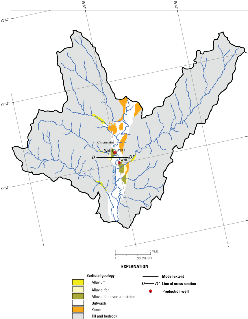
Map showing surficial geology, production wells, location of cross section, and model extent, Cincinnatus study area, New York.
Hydrogeology
The Cincinnatus study area is characterized by till-covered bedrock uplands that border a north–south trending valley drained by the Otselic River. The altitude of the surface of the shale and siltstone bedrock underlying the surficial materials is shown in figure 21; bedrock-surface altitudes range from about 890 ft in the valley to 1,970 ft in the uplands.
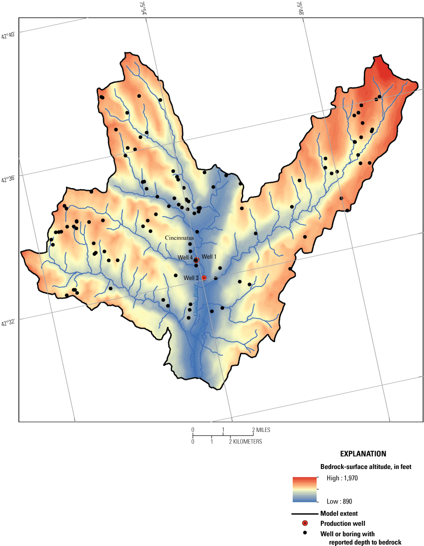
Map showing altitude of the top of the bedrock, Cincinnatus study area, New York.
There was minimal information available in the Cincinnatus study area to define the stratigraphy. Thus, the lateral extent and thickness of the lithologic units are uncertain in many areas. Surficial geology (U.S. Department of Agriculture, 2014), lithologic logs, configuration of the land-surface topography, and a regional understanding of how glacial deposits were laid down by the northward retreating ice were used to define the extent and thickness of glacial and postglacial deposits.
The valley consists of unconfined and confined sand and gravel aquifers separated by a laterally extensive fine-grained lacustrine unit; a generalized west-east geologic section through the Otselic River valley between the production wells illustrates these units (fig. 22). The unconfined aquifer consists of mostly outwash deposits, but it also includes kame deposits in several places along the valley walls. In addition, alluvial fans are present where major upland tributaries empty into the valley near the production wells (fig. 20). This unconfined aquifer is generally 30 ft thick in center areas parallel to the valley axis. Lacustrine deposits consisting of very fine sand, silt, and clay can be as much as 40 ft thick but generally are 20 ft thick in center areas of the valley. The confined aquifer, consisting of buried kame deposits, is generally thickest (20 to 40 ft) in center areas of the valley where the production wells are screened. The unconfined kame deposits and postglacial deposits along the valley walls are connected to these buried ice-contact deposits in several areas. The digital hydrogeologic maps developed as part of the present study that serve as the basis for the framework of the groundwater-flow model are available from Woda and others (2022). Data sources and the methods used to develop the hydrogeologic maps are described in Finkelstein and others (2022).
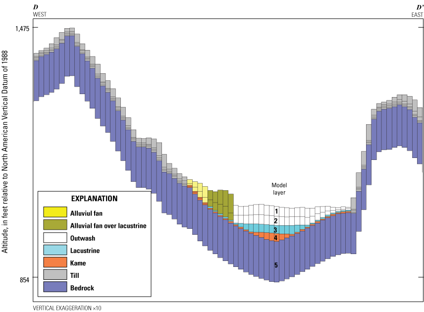
Graphs showing geologic section and model representation (line of section D–D’ is shown in fig. 20), Cincinnatus study area, New York.
Conceptually, the hydraulic connection between the confined aquifer and the overlying unconfined aquifer, and areas where the buried kame deposits connect to deposits that extend to the surface along the valley walls, are important factors for the location of the contributing areas to the production wells. The intervening fine-grained lacustrine deposits may impede vertical flow from sources of recharge to the unconfined aquifer. For the Town of Cincinnatus wells (well 1 and well 4), recharge to the unconfined kame deposits northeastward and kame deposits and alluvial fan deposits southwestward of the production wells may be an important source of water to the wells. For the Town of Cincinnatus well, well 3, recharge to the confined aquifer from kame and alluvial fan deposits along the valley wall southeastward of the well may be an important source of water. Finally, groundwater inflow from adjacent upland till and shallow bedrock may contribute to the water withdrawn by the production wells.
Development of Groundwater-Flow Model
The groundwater-flow model for the Cincinnatus study area was designed to simulate long-term, steady-state groundwater levels, flow paths, and traveltimes. A basic, manual calibration was done to six groundwater-level altitudes measured in the confined aquifer from 1945 to 2004 (USGS, 2019) at various hydrologic conditions and to a generally shallow water table that approximates the land-surface configuration in the till uplands. The altitudes of the groundwater-level measuring points were based on the altitude of the land surface determined from lidar imagery (Axis GeoSpatial, LLC, 2015; Cortland County, New York, 2017). Because of the limited number and types of observations, model calibration was considered a rough estimate of hydraulic properties. Model characteristics, including hydraulic properties and recharge rates, are summarized in table 4.
The groundwater-flow model subdivided the study area of 62.8 mi2 into 472 rows and 560 columns and included a total of 560,620 active cells. Each cell was 125 by 125 ft. In most areas the boundary of the model coincided with watershed divides in the uplands. The large extent of the model minimized the effects of these boundaries on model predictions.
Vertical discretization of the five-layered model was based on lithology (fig. 22). The unconsolidated sediments were subdivided vertically into four model layers. In the valley-fill deposits the top two layers (layers 1 and 2) represented the unconfined aquifer, which consisted mostly of outwash and kame deposits. Layer 3 in the valley represented the semiconfining unit of mostly lacustrine and some kame deposits. Layer 4 in the valleys represented the confined aquifer, which consists of kame deposits. The three production wells were simulated in layer 4. In the uplands, till deposits were represented in all four layers; shallow bedrock areas less than 13 ft from the land surface were simulated as till deposits. Layer 5, the bottom layer, represented only bedrock; the bottom altitude of layer 5 is 100 ft below the bedrock surface.
The model of the Cincinnatus study area specified the same types of boundary conditions that the Cortland and Greene study areas did to represent sources of recharge and areas of discharge. Recharge rates were applied based on the results of a soil-water-balance model (Yager and others, 2018). Mean annual recharge rates calculated by the soil-water-balance model for 2000–13 ranged spatially from 8.9 to 30.2 in/yr in the Cincinnatus study area (fig. 23). In general, lower recharge rates were computed for upland till deposits with low infiltration capacity and higher rates were computed for valley-fill deposits with high infiltration capacity. Mean annual recharge rates averaged spatially over the modeled area was 12.7 in/yr.
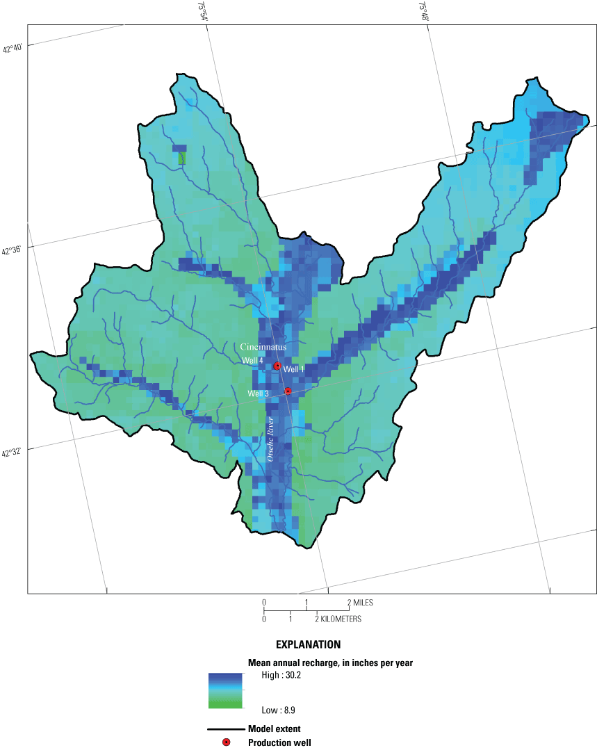
Map showing mean annual recharge rates from 2000 through 2013, Cincinnatus study area, New York.
Interactions between surface water and groundwater were simulated as a head-dependent flux boundary in layer 1 (fig. 24) by using the streamflow-routing package (Niswonger and Prudic, 2005). Stream altitudes were determined from lidar imagery. Water depth and bed thickness were set equal to 1 ft so that the top and bottom bed altitude could be determined from surface-water altitudes. Simulated streams were assigned widths ranging from 3 to 10 ft for small tributaries, as much as 20 ft for tributaries to Otselic River where they flow across the valley, and 70 ft for the Otselic River. A vertical hydraulic conductivity of 3 ft/d was used to represent bed sediments. Base flow entering the model from the Otselic River area not directly simulated was specified at the first boundary stream cell. Streamflows were specified based on base-flow statistics at the Otselic River at Cincinnatus, New York, streamgage (station number 01510000) (USGS, 2020c). The model contained 5,618 stream cells.
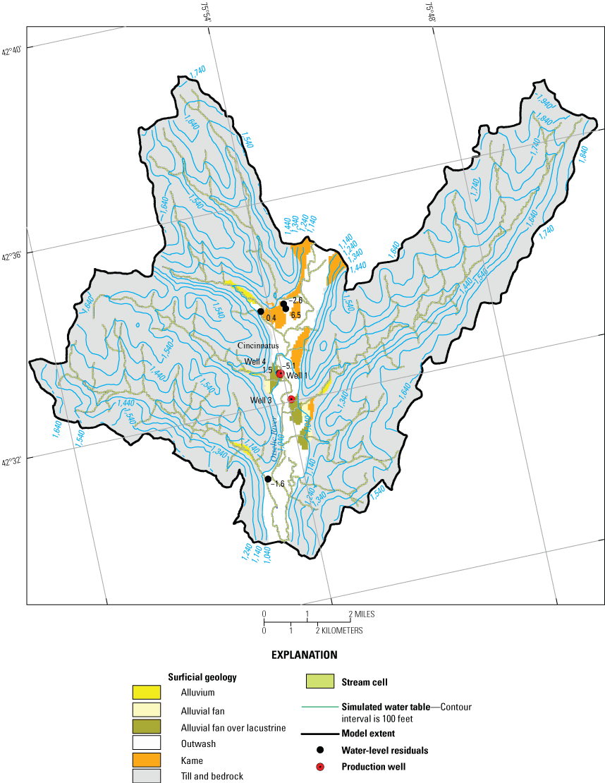
Map showing model stream cells, spatial distribution of water-level residuals, and simulated water-table contours for calibrated, steady-state conditions, Cincinnatus study area, New York.
The average annual withdrawal rate for 2010–15 from the three Town of Cincinnatus wells (table 3), which totaled only 34 gal/min, was assumed to represent long-term average rates. The three production wells are screened in kame deposits of the confined aquifer. Withdrawals from small-capacity domestic wells were not included in the model simulations because most of the pumped water is returned to the aquifer through nearby onsite septic systems.
Hydraulic conductivity values were assigned on the basis of lithology. Final calibrated hydraulic conductivity values were similar to the Greene study area (table 4). For the valley-fill deposits, final values ranged from 2 ft/d for lacustrine deposits to 200 ft/d for the outwash deposits. Till deposits were simulated as 5 ft/d. The ratio of horizontal to vertical hydraulic conductivity was 10 for all surficial deposits and 1 for bedrock.
The altitude and configuration of the simulated water table for long-term, steady-state conditions are shown in figure 24 along with the groundwater-level residuals from the limited calibration dataset. The simulated water-table contours and flow directions are consistent with the conceptual model of groundwater flow in the study area. Groundwater flows from topographically high areas and discharges to streams. In the uplands, the water table approximately parallels the land surface, and simulated groundwater divides generally coincide with watershed divides. The water-table gradient is steepest in the upland till and valley-fill deposits near the contact and flattens in the more transmissive valley-fill areas. Simulated groundwater flow in the valley-fill deposits is nearly perpendicular to the main valley stream, Otselic River, and nearly parallel to the small tributary streams that drain the uplands and become minimally gaining or losing as they flow over more transmissive valley-fill deposits. The average residual was −0.1 ft and it ranged from −5.1 to 6.5 ft.
The simulated long-term steady-state groundwater budget for the study area indicated that precipitation recharge provides 58.9 ft3/s or 82.1 percent of the total inflow. Streamflow loss accounts for the remaining inflow, 12.8 ft3/s or 17.9 percent of the total inflow. Of the total inflow, 71.6 ft3/s or 99.9 percent of the groundwater discharges to streams and the remainder, 0.07 ft3/s or 0.1 percent, is withdrawn by the production wells.
Areas Contributing Recharge
Areas contributing recharge and groundwater traveltimes to the Town of Cincinnatus production wells were determined on the basis of the steady-state model, for simulated pumping conditions, and for tracking of pathlines with the MODPATH particle-tracking program. The areas contributing recharge to the production wells for the 2010–15 average pumping rates (total of 34 gal/min; table 3) cover 0.06 mi2 (fig. 25). Although the pumping rates for the three production wells are small, the groundwater flux through the confined aquifer is also relatively small in comparison to the unconfined aquifer, thus the wells do not simulate as weak sinks. At these low pumping rates, the areas contributing recharge to each well field are only on the same side of the Otselic River as the wells. Contributing areas to the wells are from recharge originating in the upland till and near the valley-upland contact. The contributing area to the well field on the west side of the river includes small isolated areas the size of a model cell. Analysis of particle tracks indicate that recharge originating in the uplands travels through the buried ice-contact kame deposits to the wells or through the unconfined aquifer, then vertically through the relatively thin lacustrine deposits (3 to 20 ft thick) before travelling to the wells through the confined aquifer. Land cover in the contributing areas to the wells is agriculture and forested (National Land Cover Database, 2016).
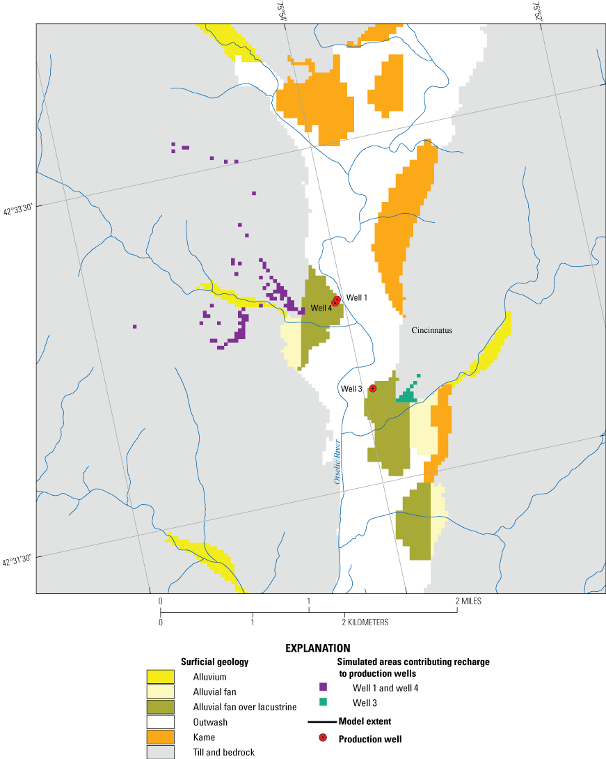
Map showing simulated areas contributing recharge to the production wells at their average pumping rates from 2010 to 2015, Cincinnatus study area, New York.
Simulated traveltime estimates from recharge locations to the production wells, based on a porosity of 0.35 for the surficial deposits and 0.05 for bedrock, are shown in figure 26. Estimated traveltimes ranged from about 3 years to 180 years; 44 percent of the traveltimes were 10 years or less. The median traveltime to the wells was 11.7 years.
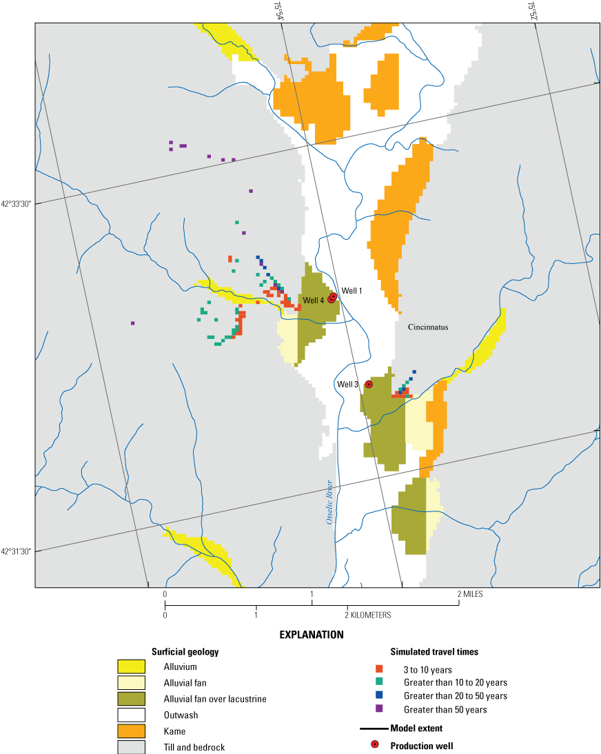
Map showing simulated groundwater traveltimes to the production wells at their average pumping rates from 2010 to 2015, Cincinnatus study area, New York.
Sensitivity Analysis
The semiconfining unit of fine-grained lacustrine deposits impedes leakage between surface sources of recharge and the confined aquifer. However, there was minimal lithologic data to determine the lateral extent and thickness of the lacustrine deposits and there were no measurements of its vertical hydraulic conductivity, which controls the connection between the unconfined and confined aquifers. A sensitivity analysis of the effects of the degree of hydraulic connection between the unconfined and confined aquifers on the simulated areas contributing recharge to the wells was done by (1) decreasing the vertical hydraulic conductivity of the lacustrine deposits and by (2) a less laterally extensive lacustrine unit near the production wells. These two scenarios were simulated with the 2010–15 total average pumping rate of 34 gal/min but also with a higher total rate of 150 gal/min (50 gal/min for each well) to increase vertical hydraulic gradients between the two aquifers. The alternate simulations are intended to provide insights into the importance of the confining lacustrine unit on delineating the contributing areas to the wells in a narrow, valley-fill setting.
The hydraulic connection between the surface sources of recharge and the confined aquifer was decreased by reducing the vertical hydraulic conductivity of the lacustrine deposits from 0.2 to 0.02 ft/d (ratio of horizontal to vertical hydraulic conductivity from 10:1 to 100:1, respectively), which is a plausible alternate value for these fine-grained, layered deposits. At the low pumping rate of 34 gal/min, the reduced hydraulic connection increased the size of the contributing area to the wells slightly (0.056 to 0.064 mi2) but the wells west of the Otselic River intercepted recharge originating in the uplands more to the northwest than west of the wells in comparison to the higher vertical hydraulic conductivity (fig. 27A). At the higher pumping rate of 150 gal/min in comparison to the lower pumping rate, the contributing area expands to capture enough water to balance the increased pumping rate, including in the till uplands on the opposite side of the Otselic River from well 1 and well 4 (fig. 27). The reduced hydraulic connection increased the size of the contributing areas to the wells for the higher withdrawal rate from 0.21 to 0.29 mi2 (fig. 27B).
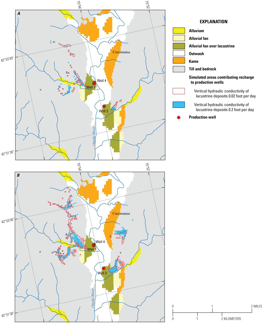
Maps showing sensitivity analysis of the effects of reducing the vertical hydraulic conductivity of the semiconfining lacustrine deposits from 0.2 to 0.02 foot per day (ratio of horizontal to vertical hydraulic conductivity from 10:1 to 100:1, respectively) on the delineated areas contributing recharge to the production wells at their total pumping rate of A, 34 gallons per minute and B, 150 gallons per minute, Cincinnatus study area, New York.
A plausible, less laterally extensive lacustrine unit near the well fields was simulated with both pumping rates. Lacustrine deposits beneath the alluvial fans west of well 1 and well 4 and east of well 3 (figs. 20 and 22) were instead simulated as kame deposits. This less restrictive connection to recharge sources caused the contributing areas to the wells to decrease from 0.06 to 0.04 mi2 at the lower pumping rate and from 0.21 to 0.17 mi2 at the higher pumping rate (fig. 28). Where the contributing areas to the wells were present, they generally coincided with the contributing area for the more laterally extensive lacustrine unit.
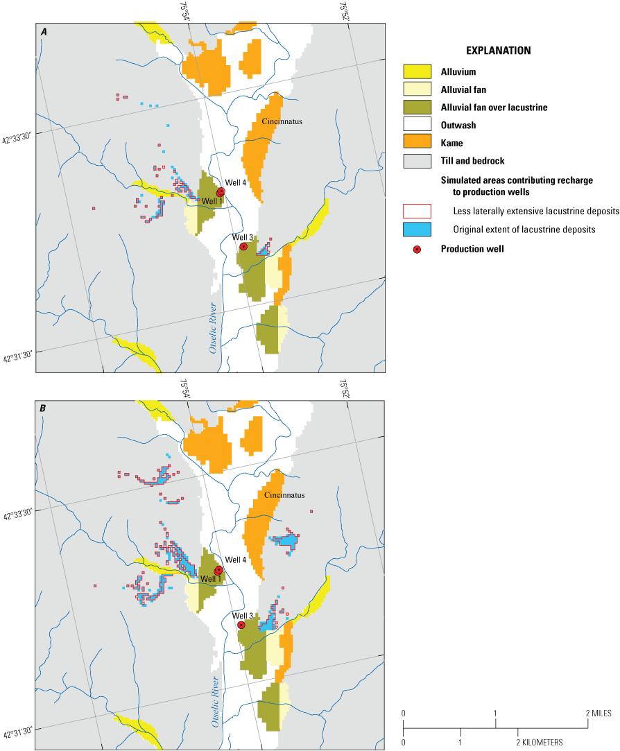
Maps showing sensitivity analysis of the effects of less laterally extensive semiconfining lacustrine deposits in comparison to the original simulated geology on the delineated areas contributing recharge to the production wells at their total pumping rate of A, 34 gallons per minute and B, 150 gallons per minute, Cincinnatus study area, New York.
Limitations of Analysis
The finite-difference numerical models of the three study areas in the Chenango River Basin are regional-scale simulations of groundwater flow, water levels, and the interaction between groundwater and surface water. Simplification included consolidating parameters that represented hydraulic properties and boundary conditions into homogenous units and assigning these parameters to groups of model grid cells sized 125 by 125 ft. Groundwater flow in the upland till and bedrock was greatly simplified. Although hydraulic conductivity values can be highly variable in till deposits, only a few values were used to represent these unsorted materials. Groundwater flow in bedrock represented the bulk flow in the regional system instead of flow through specific bedrock fractures. Thus, the models account for the overall movement of groundwater through the upland tills and bedrock before it discharges to the valley-fill deposits where the production wells are located. For these reasons, the models might not be appropriate for simulating local-scale results, but the models are useful for evaluating aquifer vulnerability to contamination at a regional scale.
The groundwater-flow model of the Cortland study area was calibrated with nonlinear regression using an extensive observation dataset collected at long-term average conditions. Uncertainty in the simulated areas contributing recharge to the production wells was based on the observation dataset and prior information and was not based on model design. Additional groundwater-level and streamflow observations and other types of field observations might help reduce the uncertainty about the extent of the simulated contributing area by increasing the precision of the parameter value estimates. Additional observations might also help to increase the number of parameters that could be estimated using nonlinear regression, thereby decreasing the need for using prior information. The resulting uncertainty analysis would then be based mostly on objective model calibration data. Uncertainty in the simulated contributing areas assumed that most plausible values are included in the analysis.
The groundwater-flow models of the Greene and Cincinnatus study areas had minimal observations for calibration and these observations represented various hydrologic conditions. Furthermore, there were limited subsurface geologic data, especially for the Cincinnatus study area, for these complex settings where the production wells tap confined aquifers. Thus, the simulation results of these groundwater-flow models may have large uncertainties. The models, however, integrate available geologic and hydrologic information and they can be modified to incorporate new information concerning the stratigraphy and recalibrated based on new field measurements of groundwater levels and streamflows.
The simulated groundwater traveltimes in all three study areas were based on uniform porosity for each of the lithologic units. An uncertainty analysis of groundwater traveltimes based on the spatial variability and the plausible range in porosity was beyond the scope of this study. However, in a steady-state model, porosity does not affect the location or size of the simulated area that contributes recharge to a well. Traveltimes also do not take into account traveltime in the unsaturated zone between the land surface and the water table.
Finally, the areas contributing recharge to the production wells are unique to the particular set of simulated pumping rates. Any changes to withdrawal rates, installation of new water-supply wells, or abandonment of wells most likely would affect groundwater-flow paths and the size and location of the predicted contributing areas.
Summary and Conclusions
The U.S. Geological Survey, in cooperation with the New York State Department of Environmental Conservation and the New York State Department of Health, began a study in 2019 to increase understanding of groundwater flow and of the areas contributing recharge to 16 production wells clustered in three study areas in the Chenango River Basin, south-central New York. The wells are screened in unconfined and confined glacial valley-fill aquifers, which are an important source of drinking-water supplies in the basin. Areas contributing recharge were delineated on the basis of numerical steady-state groundwater-flow models representing long-term average hydrologic conditions. Groundwater flow in each of the three study areas was simulated by five-layer models representing unconsolidated deposits and the underlying bedrock with a grid size of 125 by 125 feet.
In the Cortland study area, four water suppliers withdraw drinking water from 10 production wells, which supply a total average daily rate of 3.6 million gallons per day (2,478 gallons per minute [gal/min]) from an unconfined aquifer consisting of outwash sand and gravel. These production wells are operated by the City of Cortland, Town of Cortlandville, and the Villages of Homer and Hamilton. The groundwater-flow model was calibrated to 67 groundwater-level observations and 2 base-flow observations by inverse modeling using nonlinear regression. Summary statistics from the calibrated model were used to evaluate the uncertainty associated with the single, predicted contributing areas to the wells. This analysis led to contributing areas expressed as a probability distribution.
Simulated areas contributing recharge to the 10 production wells at their average pumping rates covered a total area of 6.93 square miles. Simulated areas contributing recharge extend upgradient from the wells to till and bedrock uplands and to groundwater and topographical divides. Some contributing areas include isolated areas remote from the wells, including small areas the size of a model cell. Most wells are not overlain by their contributing area because recharge travels along flow paths above and around the screen interval to the well. Land cover in the areas contributing recharge to the Cortland and Cortlandville wells includes a substantial amount of urban and agriculture land uses, but for the Homer and Hamilton well fields located in a rural area, land use is primarily agriculture and forested. Simulated groundwater traveltimes from recharge locations to the wells ranged from less than 1 year to more than 300 years; 50 percent of the traveltimes were 10 years or less. These relatively short traveltimes indicate that these wells are vulnerable to contamination from activities on the land surface.
Parameter uncertainty and its associated effects on the simulated areas contributing recharge to the wells were evaluated using a stochastic Monte Carlo analysis. Optimal parameter values and the parameter variance-covariance matrix from nonlinear regression were used to create parameter sets for the analysis. The parameter variance-covariance matrix preserves the uncertainty of the parameter estimates and the correlation among parameters from the calibrated model. Horizontal hydraulic conductivity parameters, representing the principal glacial deposits and recharge rates that were not estimated with nonlinear regression, were also incorporated into the parameter variance-covariance matrix. Because observations did not provide enough information to constrain the uncertainty of these parameters within realistic ranges around the specified values, prior information was required. The uncertainty analysis was an outcome of calibrating the model to available observations, but it also depended on information provided by the modeler. Three acceptance criteria were used to assess parameter sets so that prediction uncertainty was not overestimated: the model converged, model mass balance was 1 percent or less, and a model-fit statistic (the calculated error variance) was 2.5 times or less than the calibrated model value. Of 500 parameter sets using pumping values from the calibrated model, 470 fit the acceptance criteria. The uncertainty analysis with the average pumping rates used these 470 parameter sets with the first two acceptance criteria.
The size of the probabilistic contributing areas for the average pumping rates was larger than the size of the single, predicted contributing area for the wells because of the effects of parameter uncertainty. Thus, some areas not in the single, predicted contributing area, including additional areas with urban and agricultural land cover that have the potential to contaminate groundwater resources, might actually be in the contributing area. Low probabilities are generally in areas distant from the pumping wells and in areas where simulated streams intercepted precipitation recharge in the calibrated model. Additional areas that might be in the contributing areas include recharge originating near the wells that have relatively short groundwater-flow paths and traveltimes. For the Cortland and Cortlandville wells, areas with high probabilities (greater than 50 percent) generally coincided with the single, predicted contributing areas. For the Homer wells, areas with probabilities of greater than 25 percent generally coincided with the predicted contributing area. The probabilistic contributing area for this well field has a large spread in low probabilities because in this area of the model there were few observations to constrain estimates of the parameter values.
In each of the Greene and Cincinnatus study areas, one water supplier, the Village of Green and the Town of Cincinnatus, operates three wells that are screened near the top of the bedrock surface in a confined aquifer consisting of poorly to well-sorted sand and gravel kame deposits. This confined aquifer is overlain by a confining unit of lacustrine deposits, which in turn is overlain by a thin unconfined aquifer of sand and gravel. Average annual pumping rates in these rural settings total 169 gal/min for the Greene wells and 34 gal/min for the Cincinnatus wells. Because of the limited number and type of observations, the groundwater-flow models were manually calibrated.
Simulated areas contributing recharge to the Greene and Cincinnatus wells at their average pumping rates covered a total area of 0.35 and 0.06 square mile, respectively. The contributing areas to the Greene wells extended southeastward of the wells to the groundwater divide in the till uplands. The contributing areas also included remote, isolated areas on the opposite side of the Chenango River from the wells primarily in the till uplands. For the Cincinnatus wells with their lower pumping rates, the simulated contributing area to the wells were on the same side of the river as the wells, but they are isolated areas remote from the wells primarily in the till uplands. Land cover in these contributing areas is agriculture and forested, with the contributing areas to the Greene wells also including some urban land uses. Simulated groundwater traveltimes ranged from 3 to 300 years for the Greene wells and from 3 to 180 years for the Cincinnatus wells. Nine percent and 44 percent of the traveltimes were 10 years or less for the Greene and Cincinnatus wells, respectively. Although there are many factors that can affect traveltimes, the Greene and Cincinnatus wells are screened relatively deep and some flow paths partly travel through the lacustrine deposits, which impede the connection with surface sources of recharge.
References Cited
Axis GeoSpatial, LLC, 2015, New York tiled LiDAR: Madison and Otsego Counties, point data accessed at http://gis.ny.gov/elevation/.
City of Cortland, New York, 2020, City of Cortland, New York, wastewater treatment facility: accessed March 10, 2020, at http://www.cortlandwastewater.org/.
Cortland County, New York, 2017, Cortland County 2005 LiDAR point data: accessed at http://gis.ny.gov/elevation/.
Finkelstein, J.S., Woda, J.C., and Williams, J.H., 2022, Data sources and methods for digital mapping of eight valley-fill aquifer systems in upstate New York: U.S. Geological Survey Scientific Investigations Report 2022–5024, 21 p., https://doi.org/10.3133/sir20225024.
Friesz, P.J., 2010, Delineation and prediction uncertainty of areas contributing recharge to selected well fields in wetland and coastal settings, southern Rhode Island: U.S. Geological Survey Scientific Investigations Report 2010–5060, 69 p. [Also available at https://doi.org/10.3133/sir20105060.]
Friesz, P.J., Williams, J.H., Finkelstein, J.S., and Woda, J.C., 2022, MODFLOW–NWT groundwater-flow models used to delineate areas contributing recharge to selected production wells in unconfined and confined glacial valley-fill aquifers in Chenango River Basin, New York: U.S. Geological Survey data release, https://doi.org/10.5066/P9HU2G1K.
Garabedian, S.P., LeBlanc, D.R., Gelhar, L.W., and Celia, M.A., 1991, Large-scale natural gradient tracer test in sand and gravel, Cape Cod, Massachusetts—2. Analysis of spatial moments for a nonreactive tracer: Water Resources Research, v. 27, no. 5, p. 911–924. [Also available at https://doi.org/10.1029/91WR00242.]
Hill, M.C., and Tiedeman, C.R., 2007, Effective groundwater model calibration—With analysis of data, sensitivities, predictions, and uncertainty: New Jersey, John Wiley and Sons, Inc., 455 p. [Also available at https://doi.org/10.1002/0470041080.]
Melvin, R.L., Stone, B.D., Stone, J.R., and Trask, N.J., 1992, Hydrogeology of thick till deposits in Connecticut: U.S. Geological Survey Open-File Report 92–43, 43 p. [Reprinted as part of Connecticut Department of Environmental Protection Bulletin 20; Also available at , https://pubs.usgs.gov/of/1992/0043/report.pdf.]
National Land Cover Database, 2016, Multi-resolution land characteristics consortium: accessed May 13, 2020, at https://www.mrlc.gov/data?f%5B0%5D=category%3Aland%20cover&f%5B1%5D=region%3Aconus.
National Oceanic and Atmospheric Administration, 2020, National Centers for Environmental Information: accessed September 29, 2020, at https://gis.ncdc.noaa.gov/maps/ncei.
Poeter, E.P., Hill, M.C., Lu, D., Tiedeman, C.R., and Steffen, M., 2014, UCODE_2014, with new capabilities to define parameters unique to predictions, calculate weights using simulated values, estimate parameters with SVD, evaluate uncertainty with MCMC, and more: Integrated Groundwater Modeling Center Report Number GWMI 2014-02.
Randall, A.D., 2001, Hydrogeologic framework of stratified-drift aquifers in the glaciated northeastern United States: U.S. Geological Survey Professional Paper 1415–B, 179 p. [Also available at https://doi.org/10.3133/pp1415B.]
Randall, A.D., and Mills, A.C., 2020, Transmissivity estimated from brief aquifer tests of domestic wells and compared with bedrock lithofacies and position on hillsides in the Appalachian Plateau of New York: U.S. Geological Survey Scientific Investigations Report 2020–5087, 21 p. [Also available at https://doi.org/10.3133/sir20205087.]
Starn, J.J., and Bagtzoglou, A.C., 2012, Programs for calibration-based Monte Carlo simulation of recharge areas: Ground Water, v. 50, no. 3, p. 472–476, accessed March 2013 at https://doi.org/10.1111/j.1745-6584.2011.00868.x.
Starn, J.J., Bagtzoglou, A.C., and Robbins, G.A., 2010, Using atmospheric tracers to reduce uncertainty in groundwater recharge areas: Ground Water, v. 48, no. 6, p. 858–868, accessed January 2011 at https://doi.org/10.1111/j.1745-6584.2010.00674.x.
Terrapoint USA, 2008, New York State LiDAR Survey: Delaware and Susquehanna River Basin, point data accessed at http://gis.ny.gov/elevation/.
Town and Village of Greene, New York, 2020, Village of Greene wastewater department: accessed April 23, 2020, at https://www.nygreene.com/public-works.html.
U.S. Department of Agriculture, 2014, Soil survey geographic (SSURGO) database: U.S. Department of Agriculture, Natural Resources Conservation Service, accessed February 11, 2020, at https://cugir.library.cornell.edu/catalog/cugir-007903.
U.S. Geological Survey, 2019, USGS water data for the Nation: U.S. Geological Survey National Water Information System database, accessed December 9, 2019, at https://doi.org/10.5066/F7P55KJN.
U.S. Geological Survey, 2020a, StreamStats data-collection station report for Tioughnioga River at Cortland, New York: StreamStats—Streamflow statistics and spatial analysis tools for water-resources applications, accessed January 29, 2020, at https://streamstatsags.cr.usgs.gov/gagepages/html/01509000.htm.
U.S. Geological Survey, 2020b, StreamStats data-collection station report for Chenango River at Greene, New York: StreamStats—Streamflow statistics and spatial analysis tools for water-resources applications, accessed January 29, 2020, at https://streamstatsags.cr.usgs.gov/gagepages/html/01507000.htm.
U.S. Geological Survey, 2020c, StreamStats data-collection station report for Otselic River at Cincinnatus, New York: StreamStats—Streamflow statistics and spatial analysis tools for water-resources applications, accessed January 29, 2020, at https://streamstatsags.cr.usgs.gov/gagepages/html/01510000.htm.
Westenbroek, S.M., Kelson, V.A., Dripps, W.R., Hunt, R.J., and Bradbury, K.R., 2010, SWB—A modified Thornthwaite-Mather soilwater-balance code for estimating groundwater recharge: U.S. Geological Survey Techniques and Methods, book 6, chap. A31, 60 p., accessed August 2012 at https://pubs.usgs.gov/tm/tm6-a31/.
Woda, J.C., Finkelstein, J.S., and Williams, J.H., 2022, Interpolated hydrogeologic framework and digitized datasets for upstate New York study areas: U.S. Geological Survey data release, https://doi.org/10.5066/P96R5K5R.
World Imagery, 2018, ArcGIS online basemap, Cortland County, April 22, 2018: accessed June 5, 2020, at https://www.arcgis.com/apps/mapviewer/index.html.
Yager, R.M., Kauffman, L.J., Buchwald, C.A., Westenbroek, S.M., and Reddy, J.E., 2018, Soil-water-balance model for estimating net infiltration rates for the glaciated conterminous United States, 2000–2013—Digital products from a hydrogeologic framework for quaternary sediments within the glaciated conterminous United States: U.S. Geological Survey data release, accessed July 9, 2019, at https://doi.org/10.5066/F7HH6J8X.
Conversion Factors
U.S. customary units to International System of Units
Temperature in degrees Fahrenheit (°F) may be converted to degrees Celsius (°C) as follows: °C = (°F – 32) / 1.8.
Datum
Vertical coordinate information is referenced to the North American Vertical Datum of 1988 (NAVD 88).
Horizontal coordinate information is referenced to the North American Datum of 1983 (NAD 83).
Altitude, as used in this report, refers to distance above the vertical datum.
For more information about this report, contact:
Director, New England Water Science Center
U.S. Geological Survey
10 Bearfoot Road
Northborough, MA 01532
or visit our website at
https://www.usgs.gov/centers/new-england-water
Publishing support provided by the Pembroke and Rolla Publishing Service Centers
Suggested Citation
Friesz, P.J., Williams, J.H., Finkelstein, J.S., and Woda, J.C., 2022, Areas contributing recharge to selected production wells in unconfined and confined glacial valley-fill aquifers in Chenango River Basin, New York: U.S. Geological Survey Scientific Investigations Report 2021–5083, 48 p., https://doi.org/10.3133/sir20215083.
ISSN: 2328-0328 (online)
Study Area
| Publication type | Report |
|---|---|
| Publication Subtype | USGS Numbered Series |
| Title | Areas contributing recharge to selected production wells in unconfined and confined glacial valley-fill aquifers in Chenango River Basin, New York |
| Series title | Scientific Investigations Report |
| Series number | 2021-5083 |
| DOI | 10.3133/sir20215083 |
| Year Published | 2022 |
| Language | English |
| Publisher | U.S. Geological Survey |
| Publisher location | Reston, VA |
| Contributing office(s) | New England Water Science Center, New York Water Science Center |
| Description | Report: vi, 48 p.; 2 Data Releases; Database |
| Country | United States |
| State | New York |
| Other Geospatial | Chenango River Basin |
| Online Only (Y/N) | Y |
| Additional Online Files (Y/N) | N |
| Google Analytic Metrics | Metrics page |