

Areas Contributing Recharge to Priority Wells in Valley-fill Aquifers in the Neversink River and Rondout Creek Drainage Basins, New York
Links
- Document: Report (22.9 MB pdf) , HTML , XML
- Related Works:
- Scientific Investigations Report 2022–5024 - Data Sources and Methods for Digital Mapping of Eight Valley-Fill Aquifer Systems in Upstate New York
- Neversink-Rondout Source Water Mapper
- Data Releases:
- USGS data release - Groundwater model archive and workflow for Neversink/Rondout Basin, New York, source water delineation
- USGS data release - Interpolated hydrogeologic framework and digitized datasets for upstate New York study areas
- Download citation as: RIS | Dublin Core
Acknowledgments
The authors acknowledge Paul Friesz and John Masterson (USGS) for helpful conversations related to model design and calibration. The authors also acknowledge Robert Breault (USGS) for his help coordinating this work. We also thank Daniel Feinstein (USGS) and Alden Provost (USGS) for help with MODPATH7, and Christian Langevin (USGS) for help with MODFLOW 6.
Abstract
In southeastern New York, the villages of Ellenville, Wurtsboro, Woodridge, the hamlet of Mountain Dale, and surrounding communities in the Neversink River and Rondout Creek drainage basins rely on wells that pump groundwater from valley-fill glacial aquifers for public water supply. Glacial aquifers are vulnerable to contamination because they are highly permeable and have a shallow depth to water table. To protect the quality of these water resources, water managers need accurate information about the areas that contribute recharge to production wells that pump from these aquifers. The New York State Department of Environmental Conservation and the New York State Department of Health designated eight priority wells in this region for which water supply protection is of primary concern.
The U.S. Geological Survey, in cooperation with the New York State Department of Environmental Conservation and the New York State Department of Health, began an investigation in 2019 with the general objectives of (1) improving understanding of regional groundwater-flow system, (2) delineating areas contributing recharge to eight priority production wells, and (3) quantifying the uncertainty of these contributing areas in a probabilistic way that can be used to inform decision-making related to priority well source-water protection. To complete these objectives, a MODFLOW 6 groundwater model was created encompassing the eight priority wells and the surrounding flow system, which includes parts of the Neversink River and Rondout Creek Basins in Sullivan County and Ulster County, New York. The model was built using Python tools (such as flopy, modflow-setup, and sfrmaker) that facilitate transparent and repeatable model development using existing datasets. The model parameters were estimated with a stepwise approach using an iterative ensemble smoother implementation of the Parameter ESTimation software PEST++ (version 5.0.0). We evaluated initial “best guess” parameter bounds with a prior Monte Carlo analysis. Results of the first prior Monte Carlo analysis were used to make informed adjustments to model parameter bounds (typically resulting in expanded bounds), and a second prior Monte Carlo analysis was run to identify improved ranges for model parameters during history matching.
The history matching effort produced an ensemble of parameter values for the groundwater-flow model that spans the range of values within prior uncertainty bounds. The ensemble is informed by the historical observation data, within a reasonable range of uncertainty on those observations. This history-matched ensemble was used in a particle tracking Monte Carlo analysis to delineate the areas contributing recharge to priority wells. The groundwater-flow and particle tracking (MODPATH7) models were run once for each ensemble member. Deterministic contributing areas computed for each ensemble member were aggregated to produce maps showing the probability that a location contributes recharge to priority wells. Finally, the particle tracking Monte Carlo analysis was repeated for six pumping scenarios, representing a wide range of possible pumping levels, to incorporate uncertainty in future pumping rates related to population growth or other management decisions. Increasing pumping rates generally led to larger contributing recharge areas and larger areas of high probability that a location contributes recharge to priority wells. These maps show the overall uncertainty of the areas contributing recharge to priority wells in the study area and provide a tool for risk-based decision making for protection of well source water.
Introduction
Glacial aquifers are the principal source of water for many communities in upstate New York. The high permeability and the shallow depth to the water table in these aquifers make them highly suspectable to contamination. Sources of potential contamination are often related to land use; for example, leachate from septic systems in residential areas, stormwater runoff in developed areas, chemical spills or leaky petroleum-product storage tanks at commercial and industrial facilities, and pesticides and fertilizers from agricultural operations. Protecting these aquifers from contamination is critical in areas where groundwater use is high and alternative sources of drinking water are not readily available (Miller and others, 1998). Water managers need accurate information about the size and location of the land surface area that contributes recharge to production wells to make land-use planning decisions to reduce the risk of aquifer contamination.
The New York State Department of Environmental Conservation (NYSDEC) and the New York State Department of Health (NYSDOH) are working to reduce the risk of glacial aquifer contamination by delineating areas that contribute recharge to production wells and to encourage land-use planning within these zones. In southeastern New York, the villages of Ellenville, Wurtsboro, Woodridge, the hamlet of Mountain Dale, and surrounding communities rely on groundwater pumped from shallow valley-fill glacial aquifers for public water supply. In this region, which encompasses adjacent parts of the Neversink River and Rondout Creek drainage basins (fig. 1), the NYSDEC and NYSDOH have designated eight “priority” production wells, for which water supply protection is of primary concern. In 2019, in cooperation with the NYSDEC and the NYSDOH, the U.S. Geological Survey (USGS) began a study to characterize the regional groundwater-flow system and to delineate the contributing areas for these eight priority wells for the purpose of source water protection.
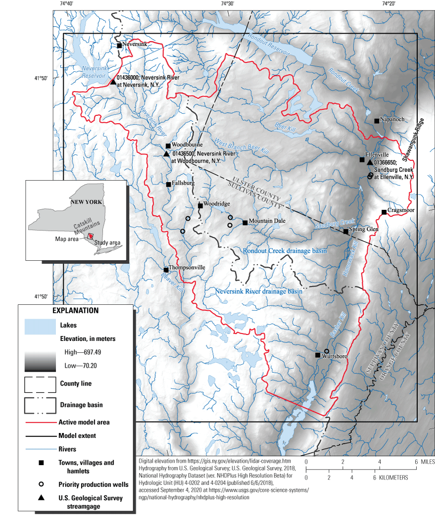
Location of the study area and model domain and other key features.
Purpose and Scope
This report describes the construction and history matching of a groundwater-flow model used for the purpose of delineating the areas contributing recharge to eight priority wells in the Neversink-Rondout (NS–RO) study area (fig. 1). The specific objectives of this study were to (1) construct a MODFLOW 6 groundwater-flow model using a Python-scripted workflow for repeatable and transparent model building; (2) do history matching using an iterative ensemble smother (iES) to produce a posterior ensemble of model parameters, conditioned on available observations, to facilitate uncertainty analysis; (3) delineate probability-based areas contributing recharge to priority wells using a Monte Carlo analysis; and (4) produce maps of results to inform risk-based land management decisions that can be used to help protect source waters for priority wells.
This report includes (1) a brief overview of the physical setting of the NS–RO study area, (2) a description of the construction of the groundwater model and history matching, (3) a description of methods used to delineate the areas contributing recharge to priority wells with probabilistic uncertainty, and (4) a discussion of limitations and assumptions. An appendix is included (appendix 1) that provides additional information about the data sources used to construct the groundwater-flow model.
Hydrogeologic Framework
The NS–RO study area covers about 183 square miles in eastern Sullivan County and western Ulster County, New York (fig. 1). The study area spans the boundary between the Appalachian Plateaus and the Valley and Ridge physiographic provinces (Fischer and others, 2004). Much of the study area is in the Catskill Mountains, which are part of the Appalachian Plateaus physiographic province. The Catskill Mountains are an uplifted, erosionally dissected plateau with high local relief. Multiple continental glaciations deeply eroded existing stream and river courses in the Catskill Mountains, incising steep valleys with narrow, flat floors that are underlain by stratified sediments (Randall, 2001). The study area is bounded to the east by Shawangunk Ridge, a high, steep bedrock ridge that is part of the physiographically distinct Valley and Ridge physiographic province (Wills and others, 2005). The total amount of relief in the study area is about 1,970 feet (ft; 600 meters).
The study area includes parts of the Neversink River and the Rondout Creek drainage basins. The Neversink River flows into the study area at the northwestern boundary at the outlet of the Neversink Reservoir. The Neversink River flows south across the study area and exits at the southeastern boundary just upstream from its confluence with Beaver Kill near Thompsonville, N.Y. The eastern parts of the study area encompasses a section of the Rondout Creek headwaters, including Sandburg Creek and its tributaries. Sandburg Creek originates near the center of the study area near Woodridge, N.Y., and flows to the northeastern boundary of the study area, above its confluence with Rondout Creek, at Napanoch, N.Y. Tributaries to Sandburg Creek include Beer Kill, West Branch Beer Kill, Homowack Kill, and several streams draining the western flank of Shawangunk Ridge.
Glacially deposited sediments fill the valleys and overlie bedrock in most of the uplands across the study area. The thicknesses of these deposits range from a few meters to more than 100 m (328 feet). Most of these materials were deposited during the advance and retreat of the last (late Wisconsin) continental ice sheet during the late Pleistocene (Randall, 2001). This ice sheet reached its terminus in northern New Jersey and Pennsylvania about 25,000 years ago and retreated northward through southeastern New York by about 21,000 years ago (Randall, 2001). The uplands in the study area are covered by a thin, discontinuous layer of till. The till consists of unsorted fine- and coarse-grained sediments (ranging from clay to boulders) deposited during the advance and retreat of glacial ice (Finkelstein and others, 2022). The valley-fill sequence consists primarily of three depositional facies:
-
proximal facies, mostly consisting of sand, gravel, and silt. These facies are commonly referred to as “kame” deposits (Miller and others, 1998, Randall, 2001; Finkelstein and others, 2022). Where saturated, these deposits form unconfined, semiconfined, and (where overlain by mid-deglacial lacustrine deposits) confined sand and gravel aquifers.
-
mid-deglacial faces, primarily lacustrine silts and clays. These layers can act as confining units in the valley-fill aquifer systems.
-
late-deglacial facies, primarily well-sorted sands and gravels, deposited as alluvium and outwash. Where saturated, these deposits generally form unconfined, semiconfined, and (where overlain by mid-deglacial lacustrine deposits) confined valley-fill aquifers.
The mid-deglacial facies, consisting of lacustrine silts and clays, are generally the most extensive and thickest of the three facies in the study area. In most valley reaches all three facies are present. In general, the surficial deposits in the valleys are late-deglacial outwash sediments that form unconfined sand and gravel aquifers. These unconfined aquifers are perched above mid-deglacial lacustrine deposits (in the valley center) and overlie bedrock (along valley walls, where the underlying sediments pinch out). The mid-deglacial confining deposits overlie proximal kame deposits that form confined (or semiconfined) sand and gravel aquifers. The base of these confined aquifers is defined by the underlying bedrock surface. In some valley reaches, only one or two facies are present. The upper and lower aquifers are connected where the confining layer is absent. A schematic representation of the valley-fill aquifer system is shown in figure 2. A more detailed description of the regional geology, including the till and bedrock uplands and valley-fill aquifers in the study area, can be found in Finkelstein and others (2022).
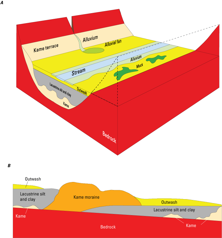
Schematic representation of a glacially deposited valley-fill aquifer; A, cross-valley view, and, B, down-valley view. Modified from Miller and others (1998).
The eight priority wells in the study area draw water from the valley-fill aquifer system. These wells are generally screened in transmissive proximal and late-deglacial deposits, such as kame, outwash, alluvium, and lacustrine sand. Information about well screen lithology is documented in table 1. Priority wells in the study area are also generally screened in unconfined or semiconfined valley-fill units, except for well SV 407 near Mountain Dale, N.Y., which is screened in kame deposits overlain by a mid-deglacial lacustrine silt and clay confining unit.
Table 1.
Neversink-Rondout priority and nonpriority production wells with 2010–2015 withdrawal rates[USGS, U.S. Geological Survey; NYSDEC, New York State Department of Environmental Conservation; gal/min, gallons per minute; NYSDOH, New York State Department of Health; --, data not available. Mean and maximum pumping rates for the period 2010-2015. Mean pumping rates were used in the model and were adjusted ±20 percent during calibration. Maximum pumping rates were used to evaluate uncertainty of the areas contributing recharge to priority wells (see figures 26–31).]
The bedrock in the study area primarily consists of Devonian and Silurian shale, sandstone, and conglomerate, and forms an undulating surface that bounds and underlies the glacial deposits in the valleys. The extents of the till-covered bedrock uplands and the valley-fill aquifers are shown in figure 3. The interior of the bedrock is assumed to be generally unweathered and sparsely fractured, but the surface of the bedrock may include a shallow zone of greater weathering and fracturing. In general, the permeability of the bedrock is low relative to the permeability of valley-fill deposits.
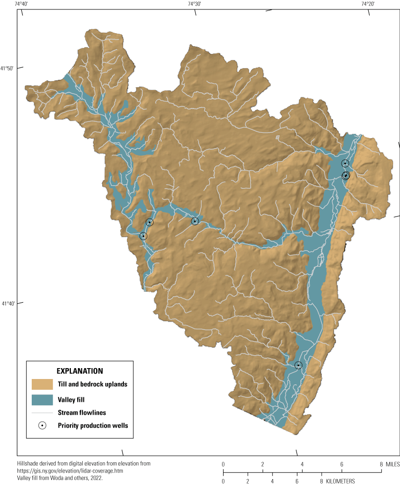
Extent of valley-fill aquifers and till-covered bedrock uplands with priority well locations.
Recharge to the upland till and bedrock is principally from infiltration of precipitation and snowmelt but also, to a lesser extent, from leakance from upland streams. The valley-fill aquifers receive recharge from a variety of sources including infiltration from precipitation, runoff from unchanneled hillsides, and leakance from tributary streams that lose water as they flow onto the permeable valley-fill deposits. Upland recharge that enters the groundwater-flow system moves laterally towards the valleys and seeps into the valley-fill aquifers at its edges.
Most of the study area boundary is defined by topographical divides in the relatively low permeability till and bedrock uplands. The topographic divides likely coincide with hydraulic divides in the groundwater-flow system, which means that there are likely no important flows of surface water or groundwater across these boundaries. For this reason, it is suitable to consider these divides as no-flow boundaries. In a few locations, the model perimeter transects river valleys that contain relatively high-permeability valley-fill deposits. These areas include the Neversink River Valley (where the Neversink River enters the model in the northeast downstream from the Neversink Reservoir and where it exits the model in the southwest below Thompsonville, N.Y.), the Basher Kill Valley below Wurtsboro, N.Y., and the Sandburg Creek Valley above Napanoch, N.Y. In these valleys there is likely some amount of groundwater flow across the model perimeter into or out of the model.
Development of Steady-State Numerical Model
A steady-state, finite-difference MODFLOW 6 (Langevin and others, 2017) groundwater-flow model was developed to simulate the groundwater-flow system in the NS–RO study area. The complete model development process, from construction through history matching and postprocessing, was scripted using the Python programming language (Van Rossum and Drake, 2009) to produce a transparent and repeatable record of the modeling process. We constructed the groundwater-flow model using several USGS-developed Python packages designed to facilitate MODFLOW model development, including flopy (Bakker and others, 2016), sfrmaker (Leaf and others, 2021), and modflow-setup. These tools were used to develop a MODFLOW 6 model and input files from source data, including shapefiles, rasters, and other MODFLOW models. Source data—representing aquifer system geometry, boundary conditions, and hydraulic properties—were read from their native formats and mapped to a regular finite difference grid using modflow-setup. The gridded model data for the desired MODFLOW packages generated by modflow-setup were then used to construct MODFLOW input files with flopy. We estimated parameters for the groundwater-flow model through history matching to be consistent with available observation data including hydraulic heads and flows representing steady-state conditions. We completed history matching using the iES implementation (White, 2018) of the Parameter ESTimation (PEST) software PEST++ (version 5.0.0; White and others, 2021). The resulting parameter ensembles facilitate uncertainty analysis through use of the pyemu (White and others, 2016) Python package.
A summary of the groundwater model design, history matching, and parameter optimization are provided in the following sections. MODFLOW input files were generated using georeferenced source data, including shapefiles, rasters, and a parent MODFLOW model. A detailed description of the geospatial source data used to construct the groundwater model is presented in appendix 1. The groundwater-flow model and the Python code used in the modeling workflow are available in the companion data release (Fienen and Corson-Dosch, 2021; https://github.com/usgs/neversink_workflow).
Model Extent and Discretization
The MODFLOW model domain consists of a uniform grid of 680 rows and 619 columns of 50-m-square cells. The model has four layers that represent the glacially deposited sediments and bedrock, with layers 1, 2, and 3 representing surficial glacially-deposited sediments—including outwash, alluvium, kame, lacustrine sediments, and till—and layer 4 representing the underlying bedrock. Layers 1–3 varied in thickness across the model domain and were spatially discontinuous. The bedrock unit, represented by layer 4, was set to a uniform thickness of 30 m. Model top elevations were derived from lidar data (U.S. Geological Survey, 2015) by sampling the mean elevation within each cell and mapping that value to the model grid. Model layer elevations were developed using a variety of information, including well construction reports, boring logs, geologic cross-section data, Soil Survey Geographic Database (SSURGO) data, and lidar data. The methods used to develop model layer elevations and thicknesses are described in detail by Finkelstein and others (2022), and the data sets are made available in the USGS data release by Woda and others (2022).
The lithology of the valley-fill aquifer systems (represented in model layers 1–3) is complex. The individual units that comprise these layers have irregular geometries that interfinger and pinch out (fig. 2, for example). The lateral continuity of the units also is variable—valley-fill facies present in one valley reach may be different than those present in another. These complex aquifer geometries were simulated using the MODFLOW 6 idomain array to specify active (idomain=1), inactive (idomain=0), and vertical pass-through (idomain=−1) cells. Vertical pass-through cells were used to route water in the model between the uppermost active and the next highest active layer; for example, if the geologic units represented by model layers 2 and 3 pinched out along the edge of a valley, vertical passthrough cells applied to layers 2 and 3 allow water to be exchanged between layer 1 and layer 4 directly, without the need for the intermediate layers to be included. This improves the computational efficiency of the model and the accuracy of the model’s physical representation of the flow system.
The geographic extent of the model was established using the topographical divides defined by 5 adjacent 12-digit hydrologic unit code (HUC) drainage basins. These drainage basins include the Upper Neversink River (020401040305), Gumaer Brook-Basher Kill (020401040201), Basher Kill (020401040203), Beer Kill (020200070503), and Sandburg Creek (020200070504). The combined extent of these drainage basins defined the active model domain with two modifications: (1) the model boundary downgradient from the Neversink Reservoir was adjusted about 0.25 mile southeast—from the top of the Neversink dam structure to its base—to improve model stability; and (2) the model extent in Basher Kill River drainage basin was truncated south of Wurtsboro, N.Y., downgradient from any priority wells to improve the computational efficiency of the groundwater-flow model. The spatial extent of the model domain is shown in figure 1.
Boundary Conditions
Hydrologic boundary conditions represent flows of water into and out of the model domain. Boundary conditions in this model include areal recharge from net infiltration percolating below the root zone, groundwater flow across the model perimeter in the valley-fill areas, stream-aquifer interactions, and groundwater extraction at wells.
Recharge
Steady-state recharge rates were estimated for each model cell using a gridded estimate of mean recharge (Yager and others, 2018, 2019). Yager and others (2019) calculated mean net infiltration recharge rates during 2000–2013 for the glaciated conterminous United States at a 250-m grid cell resolution using the Soil Water Balance code (SWB: Westenbroek and others, 2010). SWB uses spatially distributed variables, such as soil type, land use, climate data, and soil water capacity to partition precipitation into runoff, evapotranspiration, and deep infiltration. At this regional scale, all deep infiltration is assumed to enter the groundwater system as recharge.
The gridded mean deep infiltration product from Yager and others (2019) was resampled to the finer 50-m MODFLOW groundwater model grid using the modflow-setup Python package. The mean annual recharge rate across the study area for the 2000–2013 period was 14.9 inches per year. These estimates of recharge were assumed to be representative of overall steady-state conditions and were adjusted during groundwater model history matching to reflect uncertainty in the recharge estimate.
Groundwater Flow Across Model Perimeter
Groundwater flow across the model perimeter in valleys were simulated using the MODFLOW 6 specified head boundary package (CHD). CHD boundaries for this model were developed from two previously published regional groundwater-flow models (Zell and Sanford, 2020a; Zell and Sanford, 2020b). Zell and Sanford (2020a) produced 75 steady-state MODFLOW 6 groundwater-flow models that span the contiguous United States and simulate the long-term mean surficial groundwater system. The NS–RO model domain intersects parts of two Zell and Sanford (2020a) regional models. The discretization packages (DIS) and binary head output files from the two intersecting Zell and Sanford (2020a) models were combined to create a single synthetic “parent” model. NS–RO CHD values were extracted from the “parent” model head output using the modflow-setup Python package. The locations of CHD cells in the groundwater-flow model and their corresponding values are shown on figure 4.
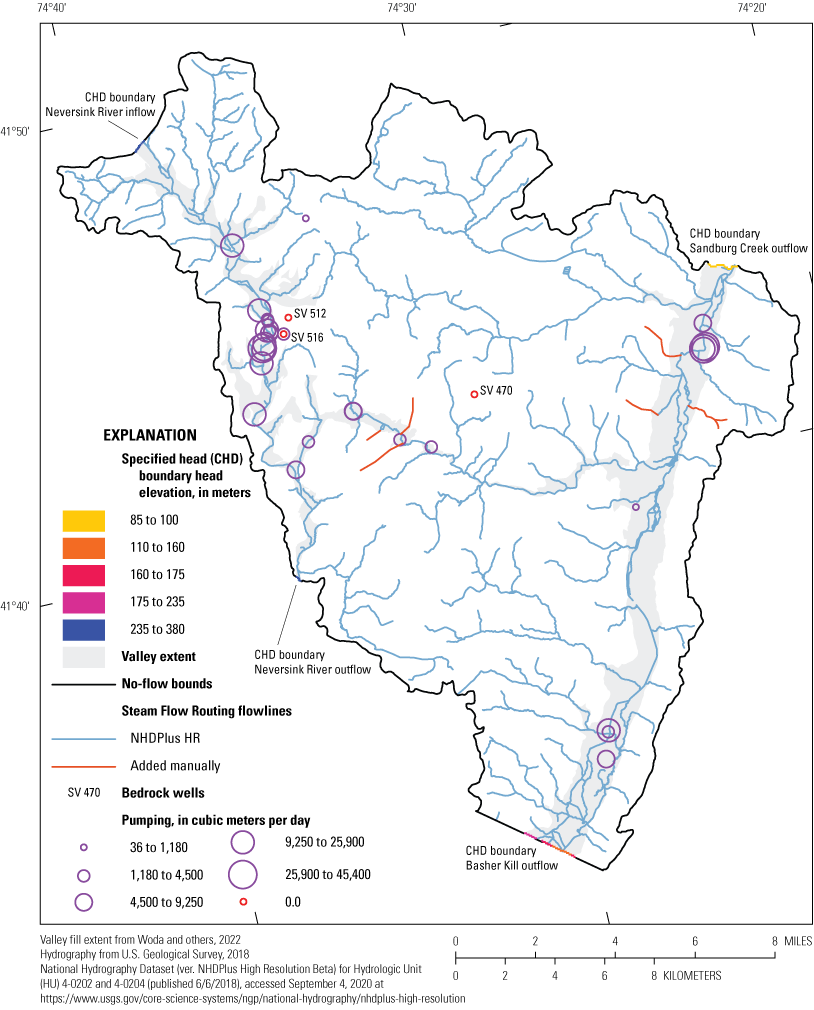
Model perimeter boundary conditions, streamflow routing (SFR) lines, and pumping wells in groundwater-flow model. Perimeter boundary cells intersecting valleys are represented by specified head (CHD) cells. Pumping well symbols (purple circles) are scaled to base realization pumping rate, except for three bedrock wells (red circles) where pumping rates were manually set to zero. CHD cell colors are scaled to CHD head elevations. Parts of the perimeter represented with no-flow boundary conditions are in gray.
Stream-Aquifer Interactions
Stream-aquifer interactions were simulated using the MODFLOW 6 implementation of the Streamflow Routing (SFR) Package (Langevin and others, 2017). The SFR package simulates stream stage and accumulated base flow by accounting for gains and losses of water in each stream cell and routing streamflow from upstream cells to downstream cells. The SFR network was developed using hydrography from the U.S. Geological Survey National Hydrography Dataset Plus High Resolution (NHDPlus HR; U.S. Geological Survey, 2018). MODLOW SFR input files were constructed using the sfrmaker (Leaf and others, 2021) Python package—a tool that facilitates construction of streamflow routing networks from hydrography data—using NHDPlus HR flowlines and the associated streamflow routing and physical property information from 4-digit HUC 0202 and HUC 0204. Additional flowlines were added to the SFR network in select locations to reduce simulated groundwater flooding near priority wells. These flowlines were added manually following topography in drainages where NHDPlus HR flowlines were not already present. The MODFLOW 6 SFR flowlines are shown on figure 4.
The Neversink Reservoir impounds flows from the Neversink River northwest of the model boundary. Outflow from the Neversink Reservoir discharges back to the Neversink River which in turn flows into the northwest part of the groundwater-flow model. Continuous streamflow is recorded at USGS streamgage 01436000 (Neversink River streamgage at Neversink, N.Y.), where the Neversink River flows into the model domain at the base of the Neversink Reservoir (fig. 1). The median daily flow rate from streamgage 01436000 (20.0 cubic feet per second; U.S. Geological Survey, 2020a) was applied as an inflow to the SFR reach of the Neversink River at the northwest model boundary (table 2). This inflow was assumed to be representative of overall steady-state conditions.
Table 2.
U.S. Geological Survey streamgages and data used for streamflow routing (SFR) inflow and base flow calibration targets.[USGS, U.S. Geological Survey; BFI, base-flow index; SFR, MODFLOW 6 Streamflow Routing package; N.Y., New York; Dates given in mm/d/yyyy. Longitude and latitude are given in North American Datum of 1983]
Period of record that overlaps with operation of downstream streamgage 01436500 (Neversink River at Woodbourne, N.Y.) and excludes period of record before the construction of the Neversink Reservoir.
U.S. Geological Survey, 2020b. Error! Hyperlink reference not valid.
Water Withdrawals
Estimates of groundwater pumping from production wells—priority and nonpriority wells—were developed from 2010 through 2015 pumping records available in the USGS Site-Specific Water-Use Data System (SWUDS) database (table 1; fig. 4). It was assumed that the 2010–2015 mean well withdrawals adequately represented pumping rates from these wells during steady-state conditions; however, pumping rates were adjusting during history matching to reflect the uncertainty in these estimates. Priority wells were assigned to model layers based on lithology. Nonpriority wells were assigned to the thickest model layer intersecting with the well open interval.
Relatively small amounts of groundwater are pumped for agricultural uses in Sullivan and Ulster Counties (Fischer and others, 2004; U.S. Geological Survey, 2020a) and no irrigation-related groundwater pumping or return flows were represented in the model. Additionally, withdrawals from smaller wells were not included. It was assumed that these wells are negligible at the scale of the model because they return most water through on-site septic systems, resulting in little-to-no net withdrawal.
Hydraulic Properties
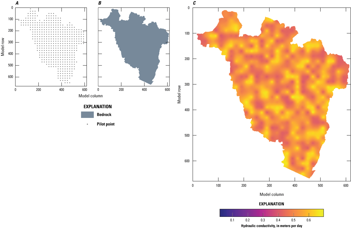
Hydraulic properties in the model were defined by zones based on lithology data and surficial geology mapping. The initial hydraulic conductivity values assigned to these zones (and initial upper and lower calibration bounds) were estimated using published regional aquifer test data (Como, 2013; Smith and Williams, 2020). The lithologic zones are shown, by layer, in panel “B” of figures 5–12. Initial (prior) hydraulic conductivities, aggregated by geologic zones, are summarized in table 3. Information about the history matching process and the development of posterior hydraulic properties are presented in the “Parameter Estimation by Ensemble History Matching” section.
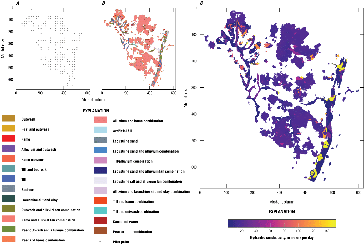
Base realization values and parameterization for horizonal hydraulic conductivity in model layer 1 with, A, pilot point network, B, lithologic zones, and, C, base realization conductivity array.
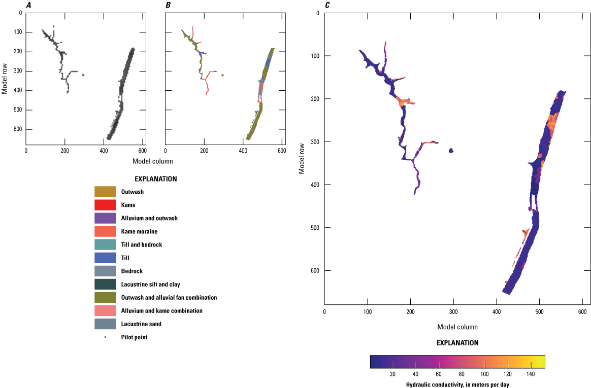
Base realization values and parameterization for horizonal hydraulic conductivity in model layer 2 with, A, pilot point network, B, lithologic zones, and, C, base realization conductivity array.
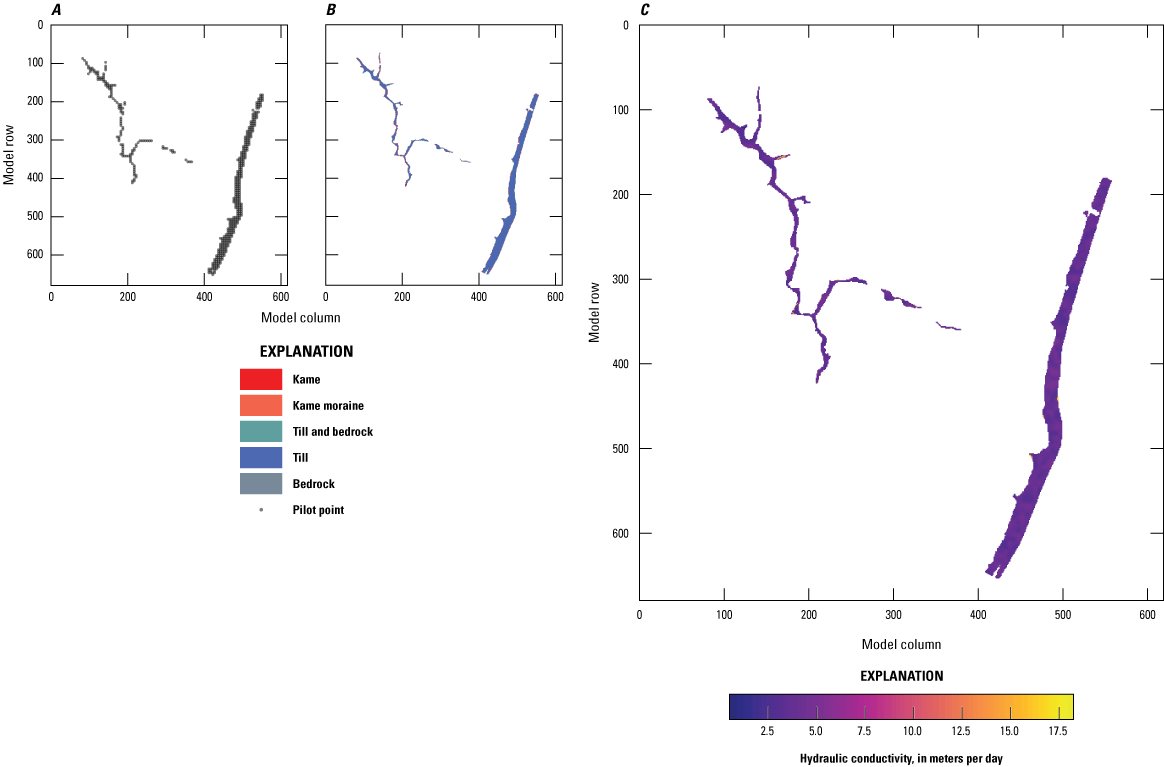
Base realization values and parameterization for horizonal hydraulic conductivity in model layer 3 with, A, pilot point network, B, lithologic zones, and, C, base realization conductivity array.

Base realization values and parameterization for horizonal hydraulic conductivity in model layer 4 with, A, pilot point network, B, lithologic zones, and, C, base realization conductivity array.

Base realization values and parameterization for vertical hydraulic conductivity in model layer 1 with, A, pilot point network, B, lithologic zones, and, C, base realization conductivity array.

Base realization values and parameterization for vertical hydraulic conductivity in model layer 2 with, A, pilot point network, B, lithologic zones, and, C, base realization conductivity array.
Base realization values and parameterization for vertical hydraulic conductivity in model layer 3 with, A, pilot point network, B, lithologic zones, and, C, base realization conductivity array.
Base realization values and parameterization for vertical hydraulic conductivity in model layer 4 with, A, pilot point network, B, lithologic zones, and, C, base realization conductivity array.
Table 3.
Summary of prior and posterior base realization hydraulic conductivities aggregated by geologic zones.[Kh, horizontal hydraulic conductivity; m/day, meters per day; Kv, vertical hydraulic conductivity; Prior, pre-history matching (or starting) value; Posterior, post-history matching value; Base, base realization representing the central tendency of the posterior parameter distribution; Min, minimum; Max, maximum; Anisotropy values are unitless]
Parameter Estimation by Ensemble History Matching
We did history matching to systematically adjust parameter values in the model such that they were consistent with historical observations of model outputs including hydraulic head and base-flow values. The general history matching approach follows Bayes’ theorem (Tarantola, 2005) for parameter estimation. In this approach, we start with a prior estimate of model parameters and their credible range (in other words, uncertainty). These prior parameter values and uncertainty are informed by expert knowledge, literature values, and available direct measurements. Through a systematic conditioning step, both the parameter values and the uncertainty are updated to be consistent with observations that correspond to model outputs. This step is referred to as an “update” and results in a posterior set of parameter values and uncertainty range (“posterior” meaning “after the update”). There are many algorithms that can be used to complete this conditioning, and for this work we used the iES implementation (White, 2018) of PEST++ (version 5.0.0; White, 2018; White and others, 2021).
iES is an ensemble method, meaning at every stage of analysis, an ensemble of parameter sets (realizations) consistent with their inherent uncertainty and the assumed uncertainty in the observations is available. Each parameter set from this ensemble can be run through the model to provide a range of model outputs. iES uses empirical correlations between parameter and observation ensembles to iteratively reduce the uncertainty and discrepancy between model outputs and observations. iES produces a posterior parameter ensemble that is characteristic of the inherent uncertainty in the parameters and model and conditioned on the available data. This ensemble can then be used for predictive analysis—in this case, the delineation of probabilistic areas contributing water to priority production wells with results that span the likely range of outcomes.
Observation Data
An observation dataset was developed to compare model outputs with field measurements of the system to facilitate ensemble-based history matching. Historical water-level measurements were obtained from the National Water Information System (NWIS) and NYSDEC water well completion reports (New York State Department of Environmental Conservation, 2020). Only a single water-level measurement was available in the NWIS database (at site 414525074360601; U.S. Geological Survey, 2020a). Where present, multiple hydraulic head measurements were averaged across time to derive a single, steady-state value for a given location. In instances where water-level measurements were reported as depth to water below land surface, water-level elevations were computed by subtracting depth to water values from the model top elevation. This subtraction is accompanied by substantial uncertainty given the steep terrain and the resolution of the elevation data informing the model’s top. In total, 448 hydraulic head targets were used for history matching. The single NWIS measurement includes more accurate elevation information than the NYSDEC measurements; however, the need to average over time causes enough uncertainty that the entire group of hydraulic head measurements was assumed to have the same uncertainty. This assumed hydraulic head measurement uncertainty was used to assign weights to hydraulic head observation for the history matching. During history matching, hydraulic head observations were compared against transmissivity-weighted hydraulic heads simulated by the model at the location of the observation well.
Steady-state base flows were computed from continuous records at two USGS streamgages 01436500 (Neversink River at Woodbourne, N.Y.), and 01366650 (Sandburg Creek at Ellenville, N.Y.). Long-term mean base-flow index (BFI; the average proportion of streamflow that is base flow) was computed using the USGS StreamStats web application (U.S. Geological Survey, 2020b). Mean annual flow rates were multiplied by the BFI values to compute an estimate of steady-state base flow (table 2). At streamgage 01366650, mean annual flow rates were computed using the entire period of record (October 1, 1957–September 29, 1977). At streamgage 01436500, only data collected after the construction of the Neversink Reservoir were used to compute mean annual flow rate (October 1, 1954–September 30, 1993). It was assumed that base flow computed over these periods is representative of long-term steady state conditions.
Land-surface elevations were also used as inequality targets on a grid every 50 model cells in each direction. We initially met a challenge common to this setting of hydraulic head solutions above the land-surface elevation (in other words, flooding) in early versions of the model, particularly before history matching. The locations of calibration targets are shown on figures 13–15.
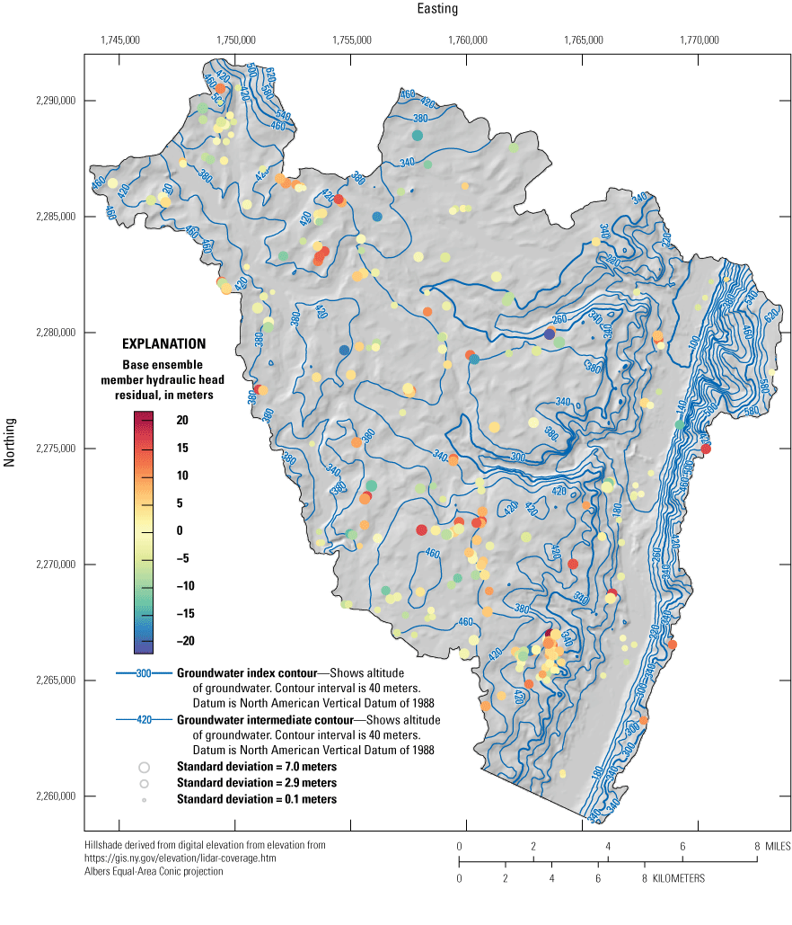
Spatial distribution of hydraulic head residuals (observed minus simulated) for the posterior parameter ensemble. Symbol colors are scaled to the base realization residual. Blue values indicate simulated values that are higher than observed. Symbol sizes are scaled to the standard deviation of the residual across the posterior parameter distribution; residuals are in meters. Water-table contour interval is 40 meters.

Spatial distribution of flux residuals (observed minus simulated) for the posterior parameter ensemble. Symbol colors are scaled to the base realization residual. Blue values indicate simulated values that are higher than observed. Symbol sizes are scaled to the standard deviation of the residual across the posterior parameter distribution; residuals are in cubic meters per day. Water-table contour interval is 40 meters.
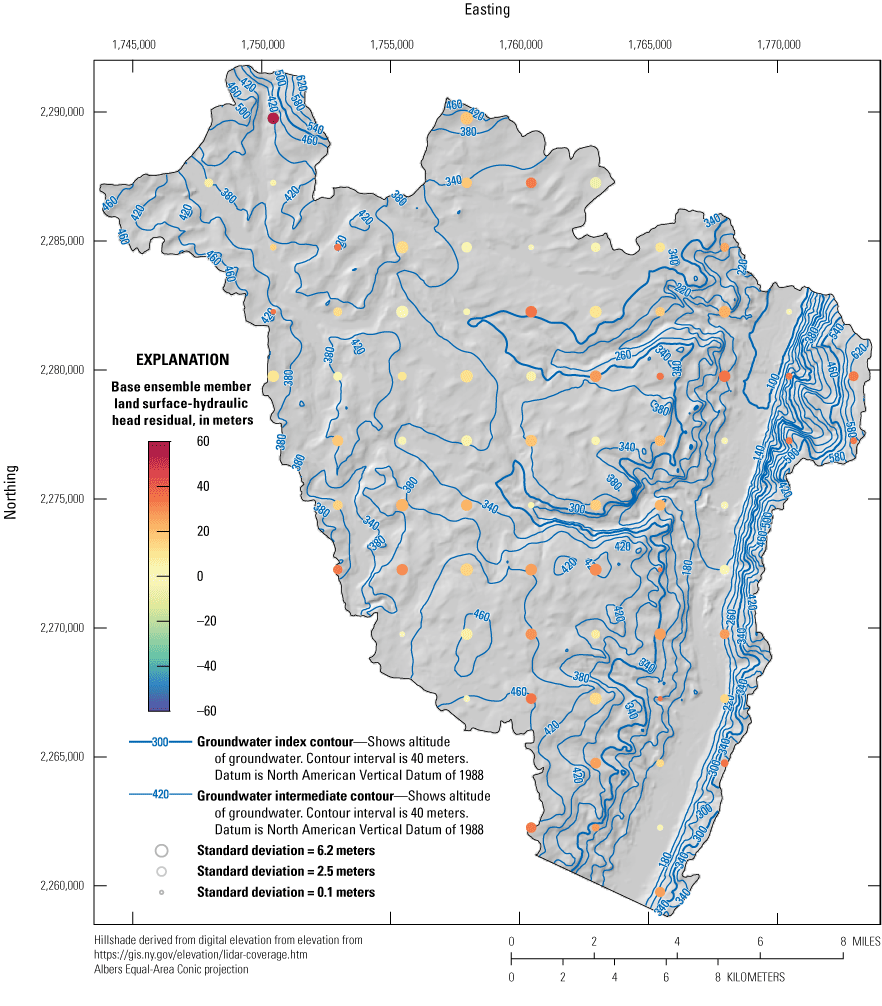
Spatial distribution of land surface inequalities (land-surface elevation minus simulated hydraulic head) for the posterior parameter ensemble. Symbol colors are scaled to the base realization residual. Red values indicate simulated hydraulic head elevations below land surface. Symbol sizes are scaled to the standard deviation of the residual across the posterior parameter distribution; residuals are in meters. Water-table contour interval is 40 meters.
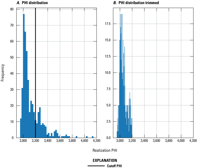
We grouped the observations in three groups: flux, hydraulic head, and land surface. We assigned initial weights based on a general assumption of the observation quality (table 4), which corresponded to a coefficient of variation of 10 percent for flux observations, and standard deviation of 5 and 10 m for the hydraulic head and land-surface observations, respectively. These assumptions are qualitative and result in an imbalanced objective function (the squared sum of residuals between model outputs and observations, each multiplied by their weight, and referred to as the ‘PHI’ value; fig. 16A). Subjectively, we judged that a reasonable balance of the objective function is 20 percent for hydraulic heads, 30 percent for flux, and 50 percent for land surface. This results in the balanced objective function in figure 16B with adjusted weights shown in table 4. The adjusted weights imply a reversal of standard deviation between hydraulic head and land-surface observations (11.2 and 2.4 m, respectively). Furthermore, the implied standard deviation for the two flux observations decreased dramatically because of this rebalancing; however, without adjusting the weights, the history matching algorithm would largely ignore the flux observations, allowing great variability and not constraining the overall water balance of the model. While many hydraulic head observations were available, they are individually subject to substantial uncertainty as discussed previously.

PHI distribution, A, before and, B, after rebalancing the objective function
Table 4.
Summary of observation data, observation groups, and initial and rebalanced weights.Stepwise Estimation of Model Parameters
Model parameters that are estimated in the history matching process are those for which we assume are informed by the observations. In choosing which parameters to allow to be adjustable through history matching, we acknowledge that any parameters not allowed to be estimated through history matching are assumed perfectly known. In this section, we outline the strategy for selecting the parameters to adjust and estimate in the history matching process. We then describe the approach for evaluating the uncertainty of parameters and observations to set initial parameter values and then the algorithm for history matching.
Parameterizing the Model
We followed the technique proposed by White and others (2020) to use multiple scales of variability in the parameterization. We typically used multipliers to allow adjustment at multiple scales—for example, single multipliers applied at the model layer scale combined with zone-wise multipliers applied to local areas (zones) within the model, in the case of parameters representing hydrogeologic properties (for example, hydraulic conductivity). Within zones, multipliers on pilot points (Doherty, 2003) were used to allow for finer-scale variability in hydraulic conductivity and recharge. Table 5 shows the categories of parameters and the number of adjustable parameters for each type. For horizontal and vertical hydraulic conductivity, we assigned zone-based homogeneous multipliers based on the mapped lithologic zones. Additionally, pilot points were placed every 20 cells in layers 1 and 4 and every 5 cells in layers 2 and 3. The higher frequency in layers 2 and 3 was to accommodate the irregular geometry of the geological zonation in those layers. The hydraulic conductivity zones and pilot point networks are displayed in panel “C” of figures 5–12. In a similar multiscale approach, we implemented a single recharge multiplier for the entire recharge array to allow for relatively large-scale adjustment, augmented by pilot points to allow for finer scale adjustment. The recharge pilot points were also placed every 20 model cells. The recharge pilot points are collocated with the layer 4 hydraulic conductivity pilot points as displayed in figure 17. The final parameters we implemented are the pumping rate in each well (as a multiplier) and a multiplier for the SFR streambed conductance by reach.

Estimated annual recharge to the groundwater system. Recharge rates shown are from the base realization, representing the central tendency of the calibrated posterior parameter distribution. The mean annual recharge rate across the study area is 14.1 inches per year.
Table 5.
Summaries of initial parameter values and bounds during the prior Monte Carlo, expanded Monte Carlo, and iterative ensemble smoother history matching, aggregated by parameter type.[iES, iterative ensemble smoother; SFR; MODFLOW 6 Streamflow Routing package]
Using Uncertainty Analysis to Set Initial Values
An initial prior Monte Carlo analysis was completed on the parameterized model. A parameter ensemble was generated assuming a normal distribution of values and that the parameter bounds represent a spread of 4 standard deviations (in other words, 95 percent confidence) about the initial parameter values, as shown in table 5 in the section “Prior Monte Carlo.” The bounds were intentionally limited to keep parameters within initial ranges based on literature values. This was particularly problematic for the bedrock hydraulic conductivity values that assume deep, generally unweathered, and sparsely fractured bedrock when, in reality, the bedrock units include a shallow zone of greater weathering and fracturing that must be represented by the same unit.
The initial parameter bounds were evaluated by comparing model outputs from the ensemble of parameter samples in the prior Monte Carlo against observation data. We used an ensemble approach to sample the “noise” of the observations such that each realization uses a set of observation values sampled from a normal distribution with the mean being the reported observation value and the standard deviation being a user-defined variance representative of the uncertainty of the observations (table 4).
The left column in figure 18 shows histograms for several representative observations. The blue histograms represent model outputs from the ensemble of parameter samples in prior Monte Carlo. The orange histograms represent the ensemble of observation values, with the vertical solid line representing the reported observation value, and the vertical dashed lines representing ±1 standard deviation of the observation ensemble. While observations A and B show that flux is overestimated in one location and underestimated in another, observations C and D show that with the initial parameter assumptions, hydraulic heads are often too high; in the case of observation D, hydraulic head is 25 to 75 m higher than land surface. As a result, we expanded the bounds for hydraulic conductivity parameters by zone and reran the Monte Carlo analysis resulting in generally lower heads (the middle panels of fig. 18) although with relatively minor changes to the flux residuals. Based on this improvement, we used the parameter ensemble from the expanded Monte Carlo as both starting parameter values and upper and lower bounds for the history matching. The 25th, 50th, and 75th quantiles from the expanded Monte Carlo parameter ensemble were assigned as the lower bound, initial parameter value, and upper bound for history matching, respectively. These values are summarized in table 5 in the section “iES start.”
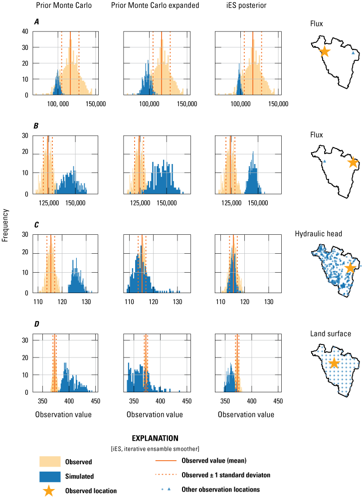
Histograms for selected observations showing model performance with respect to observed values for the “prior Monte Carlo” (left column), “expanded bounds Monte Carlo” (first column from left), and final “iES posterior” (first column from right) parameter ensembles. The location of the observation is shown in the right column. Ensemble results for, A, flux observation at U.S. Geological Survey (USGS) streamgage 01436500 (Neversink River at Woodbourne, N.Y.), B, flux observation at USGS streamgage 01366650 (Sandburg Creek at Ellenville, N.Y.), C, hydraulic head observation at well U 3717, and, D, land-surface inequality at model row 250, column 300. Blue histograms show the distribution of model outputs and orange histograms show realizations of the observation value based on the reported observation (obs mean) and a subjectively defined standard deviation.
History Matching with the Iterative Ensemble Smoother (iES)
We selected the iES (White, 2018) as implemented in PEST++ (White and others, 2021) for history matching. This technique builds on the Monte Carlo approach by evaluating an ensemble of parameter values, yielding a residual vector and calculating a weighted objective function for each member of the parameter ensemble. From this information, the algorithm calculates an updated ensemble of parameters to evaluate, and iterations are done until a posterior conditioned ensemble is obtained. This results in an ensemble of objective function values from iteration to iteration (fig. 19). In figure 19, the red curve represents a base ensemble member that is taken as representative when a single realization is desired. The iES approach does not depend on local linearization of the inverse problem so inequality observations are possible. In this case, we defined water levels at the land surface on a regular network as inequality observations for the land-surface observation group. If the inequality is not invoked (in other words, if the model output hydraulic head elevation is lower than the collocated observation of land-surface elevation) then the weight assigned to this observation is 0.0 and thus the residual does not play a role in the objective function calculation. However, if the simulated hydraulic head exceeded these elevations, a quadratic penalty in the objective function was incurred at their assigned weights. Furthermore, the observation noise distributions allow flexibility in the algorithm to consider the uncertainty of the observations which, as discussed previously, is considered significant in this case where we have many observation values but none of them may be perfectly representative (for example, uncertainty in their location, timing versus the steady state model, and other aspects).

Summary of ensemble (black lines) and base (blue line) objective function progress by iterative ensemble smoother (iES) iteration.
We selected the results of the second iES iteration as optimal based on a subjective judgement that the objective function had lowered to an acceptable level of fit while still retaining variability in the ensemble thus still capturing uncertainty in the system. As an additional step, we applied a rejection sampling process in which objective function values that are unacceptably high are trimmed from the ensemble. As shown in figure 20, a PHI cutoff was selected that removed anomalously high PHI results and results in an approximately normal distribution of PHI results. Figure 21 shows the correspondence between model outputs and observations, broken down by group. These results are shown to have little bias and low variance relative to the uncertainty of the observations. In figure 21, the blue symbols show fit for the representative base model while the bars indicate the 95-percent credible interval as calculated from the trimmed ensemble. Figure 18 shows the posterior ensemble of model outputs compared with the ensemble of observation values, the distribution of outputs and observations are consistent with their uncertainty. Generally, for the examples shown, the distributions of model outputs and observation uncertainty overlap with similar mean values.
Figures 13–15 show the spatial patterns of the residuals for the hydraulic head, flux, and land-surface observation groups, respectively. In each figure (13-15), the color of the symbol indicates the residual value (defined as observed value minus simulated value) for the base ensemble member, and the size of the symbol indicates the standard deviation of the residuals for all the ensemble members. In figure 14, one residual value is positive and one is negative. In figure 13, the residuals are positive and negative as well, highlighting that while there are some clusters of simulated values exceeding observed and vice versa, there is not a consistent spatial pattern that might indicate a structural issue with the model or the estimated parameters (for example, if all valleys were simulated as flooded). This mixed pattern of residuals is the desired outcome from history matching and indicates that the results are generally unbiased. The pattern is different for the land-surface residuals in figure 15. In this case, there are very few negative residuals and nearly all are biased such that the simulated results are lower value than the observed. Because these are inequality constraints and were intended to prevent parameters from driving the solution to simulate hydraulic heads higher than land surface, this bias is the desired outcome.
Comparison of posterior parameter ensembles, A, before and, B, after anomalously high PHI values were trimmed during rejection sampling.
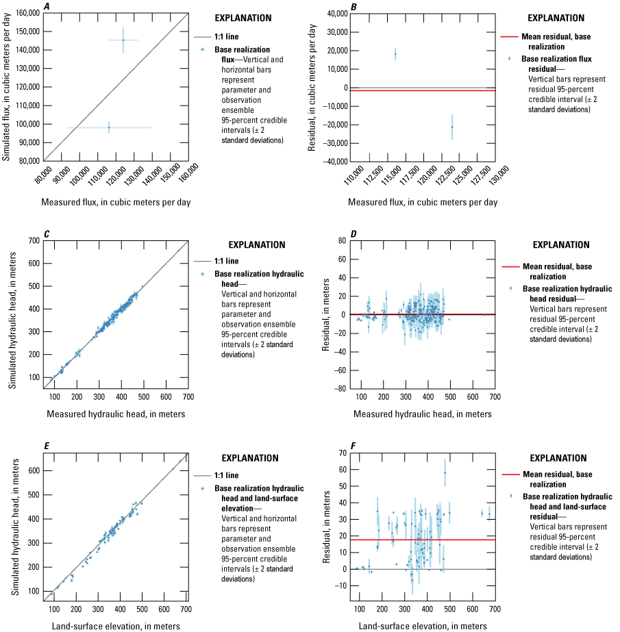
Relations among observed and simulated flux, hydraulic head, and land-surface inequalities, and plots of residuals compared to observed values. Points represent base realization values (the central tendency of the posterior parameter distribution), and the bars represent the 5th–95th percentile ranges of the observation and posterior parameter distributions. Simulated and observed values of, A, flux observations, C, hydraulic head observations, and, E, land surface inequalities. Residuals and observed values of, B, flux observations, D, hydraulic head observations, and, F, land-surface inequalities.
Base Realization
The final values of the “base” realization represent the central tendency of the posterior parameter distribution (White and others, 2021). This realization differs from the other realizations that are obtained by making a stochastic sample using the bounds of the initial parameter values. Instead, the base realization is initially made up of the specific starting values provided to PEST++. As a result, this realization starts at values that are considered “most likely” by the users. This realization is then subjected to adjustment during each iteration of the iES algorithm, but the central tendency typically remains, and this single realization typically is less variable than the other realizations. In this section, we present the representative base realization model properties, including hydraulic conductivities and boundary conditions that are representative of the optimal iES ensemble. We also discuss model results that were simulated using base realization parameters, including the simulated water balance, water table, and streamflow. For the analysis of areas supplying recharge, however, the entire ensemble is used to be sure that rather than focusing on central tendency, we are exploring the range of outcomes consistent with prior knowledge of the parameters and the information from the observation data.
Hydraulic Conductivity
Base realization hydraulic conductivity arrays, zones, and pilot points are shown in figures 5–12. Horizonal hydraulic conductivity arrays from model layers 1–4 are shown in figures 5–8, and vertical hydraulic conductivity arrays from model layers 1–4 are show in figures 9–12. Base realization hydraulic conductivities, aggregated by geologic zones, are summarized in table 3. Base realization horizonal hydraulic conductivity values were generally larger than vertical values, but in some areas of model layers 1 and 3, adjusted vertical hydraulic conductivities (Kv) were larger than horizonal conductivities (Kh). Prior Kv values were set equal to 10 percent of Kh values. This relation was not enforced during history matching, and Kv and Kh were adjusted independently. These areas were limited to relatively small areas in layer 1 (in the highly permeable [sand, outwash] and [or] generally unstructured [kame, till] deposits) where it is not unreasonable for Kv to be similar or slightly larger than Kh. An analysis of model anisotropy—the ratio of Kh to Kv—aggregated by lithologic zone is shown in figure 22. A simple sensitivity analysis was done to evaluate the relative importance of cells with anisotropy greater than 1 to overall model performance. A version of the base realization model was created where Kh was increased to equal Kv in all cells where anisotropy was greater than 1.0. This adjustment did not result in an appreciable change to model performance (less than 0.5 percent change in the objective function PHI), so the few cells with anisotropy greater than 1.0 were allowed to remain for the rest of the analysis.
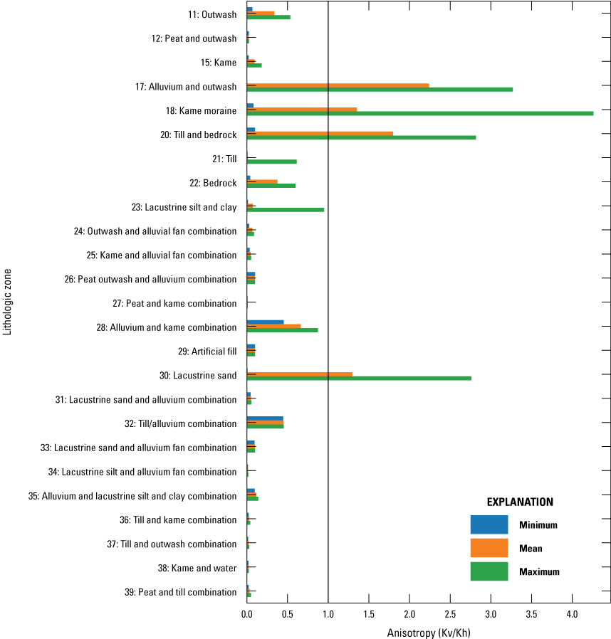
Summary of base realization anisotropy—the ratio of horizonal (Kh) to vertical (Kv) horizontal conductivity—in the groundwater-flow model. Anisotropy values less than 1 indicate Kh>Kv. Anisotropy values greater than 1 indicate Kh<Kv.
Boundary Conditions
The base realization recharge array and parameterization is shown in figure 17. The base realization recharge resulted in slightly greater variability from Yager and others (2019) and had a slightly lower mean recharge rate of 14.1 in/yr across the study area. Well pumping rates were adjusted during calibration, but base realization pumping rates compare closely to reported values, with a mean difference of just 1.4 percent from initial pumping rates among all wells. Figure 23 shows the simulated base flow in the streams represented by the SFR package throughout the model. Negative values indicate flow into the streams from the groundwater-flow system (gaining streams), and positive values indicate flow from the streams into the groundwater-flow system from the streams (losing streams). Most of the model domain is characterized by gaining streams, although near the outlet of the Neversink Reservoir in the northwest corner of the model, in some of the steepest valley wall slopes, and at valley margins, losing streams are simulated. Some dry SFR reaches were simulated in upland areas and likely represent intermittent, low-order streams.
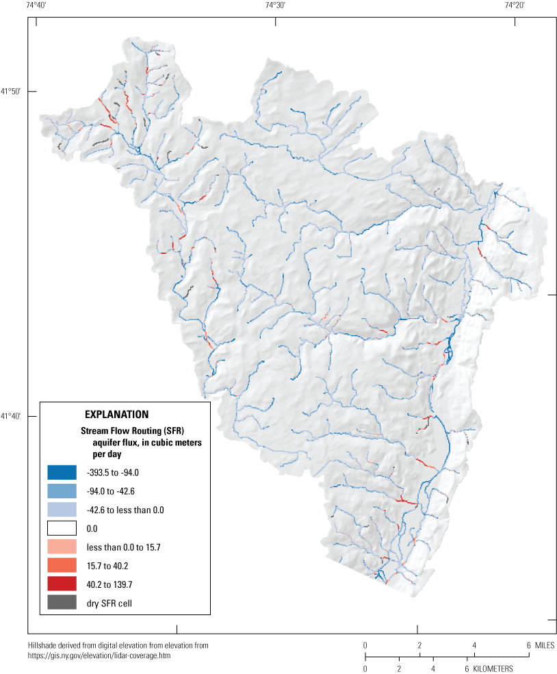
Base realization aquifer flux in Streamflow Routing (SFR) cells. Negative (blue) values are gaining (aquifer discharge to SFR) and positive (red) values are losing (SFR discharge to aquifer). White cells have no aquifer flux and gray cells are dry.
Water Balance, Water Table, and Streamflow
The main components of the water balance, as simulated by the MODFLOW 6 model, are presented in figure 24 for the base realization. As expected from the conceptual model of the system, the main inflow component is recharge and the main outflow component is discharge to streams represented by SFR. Smaller inflow components are recharge from streams represented by SFR and inflow at CHD boundaries. The smallest outflow component is the water removed through well pumping, followed by flow out through CHD boundaries. As required in the formulation of MODFLOW 6, the fluxes in and out of the model balance to zero.
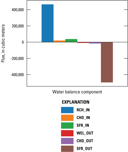
Base realization groundwater model mass balance.
The simulated water table, where hydrostatic pressure is equal to atmospheric pressure, is shown in figure 25 as contours that depict a muted representation of the land-surface elevation, stylized in shaded gray. Figure 25 also shows areas where the model is “flooded”—locations where the simulated water table is higher than the top of the model. Such simulated “flooding” is a common issue in valley-fill regions with substantial areas of thinly covered bedrock. In reality, flooded areas may correspond to wetlands where groundwater is discharging at the land surface. In early versions of the model, literature-based parameter values, particularly for the bedrock, resulted in extensive simulated flooding. Furthermore, some areas with inadequate SFR representation resulted in the model’s inability to convey water from low-lying areas into streams. With the refined stream network and parameters informed through history matching, the extent of flooding is limited to areas deep in the valleys and some highlands that are generally coincident with wetlands and ponds or lakes. Routing of water simulated above land surface could be implemented through the MODFLOW 6 unsaturated zone flow (UZF) package (Feinstein and others, 2020); however, we judged the extent of flooding to be sufficiently limited that the additional package, accompanied by more computational complexity, was not necessary.

Base realization simulated flooding.
Providing an Ensemble for Monte Carlo Analysis of Areas Contributing Recharge
The end result of the history matching effort was an ensemble of parameter values for the groundwater-flow model that spans the range of values within prior uncertainty bounds and that also is informed by the historical observation data, within a reasonable range of uncertainty on those observations. We carried this ensemble through to the simulations to delineate the areas contributing recharge by running the groundwater-flow and particle tracking models for each ensemble member, as we discuss in subsequent sections.
Simulation of Areas Contributing Recharge and Prediction Uncertainty Analysis
We completed a Monte Carlo analysis to simulate the flow field using the posterior history-matched ensemble of groundwater-flow model parameters to determine the probability of a recharge location being in the contributing area of the priority wells. This section describes the methods used for delineating priority well recharge areas and of the uncertainty analysis of these predictions.
Probabilistic Areas Contributing Recharge
The areas contributing recharge to the priority production wells were delineated using the groundwater-flow model and a particle-tracking simulation. Parameter sets produced by the history matching process were used to run MODFLOW. The unique flow field generated by each parameter realization and MODFLOW were then used to build MODPATH7 (Pollock, 2016) particle tracking input files. For the MODPATH7 simulations, one particle was placed in each cell in the uppermost active layer (in the same way that recharge is applied to the model) at the beginning of the simulation. Particle tracking was then run in the forward direction. The movement of the particles simulate the movement of recharge through the aquifer system, moving downgradient toward sinks (such as wells) and other model boundaries. MODPATH7 tracks the movement of the particles during the simulation and records where they terminate at model sinks. In this study, we instructed particles to stop when they met weak sink cells, which was necessary because some of the priority wells in the model are weak sinks (see Abrams and others, 2013 for additional information about weak sinks). At the conclusion of the particle-tracking simulation, the particles that terminated in priority well sinks were traced back to their starting locations and mapped to the model grid. This produced a single, deterministic map of the model cells that do (and do not) contribute recharge to priority wells.
Prediction Uncertainty Analysis
Results of the history-matching process produced an ensemble of 500 groundwater model parameter realizations that account for both model parameter and calibration data uncertainty. Of these 500 parameter realizations, 142 were trimmed from the ensemble during rejection sampling analysis to remove anomalously high PHI values (fig. 20) and thereby parameter sets that result in unrealistic groundwater levels and streamflows. The remaining 358 parameter realizations were used to complete a Monte Carlo analysis to quantify the uncertainty of the contributing recharge area to priority water-supply wells. The MODPATH particle tracking process, described in the “Probabilistic Areas Contributing Recharge” section, was repeated for each of the 358 realizations in the history-matched parameter ensemble. Deterministic contributing recharge areas produced from these repeated runs were used to calculate the probability of a location being in the area contributing recharge to a priority well.
In the history matching part of the project, best estimates of mean water use were used for the well package in MODFLOW 6; however, these estimates are typically not at the highest range of capacity for the wells, in particular for the priority wells (table 1). As a result, variations in pumping rates related to population growth and other future decisions were added as an additional consideration beyond model parameters that contribute to the overall uncertainty of the contributing recharge area. The uncertainty in pumping rates was represented using six pumping scenarios:
-
Baseratio: priority well pumping rates only adjusted by history matching;
-
Maxratio: priority well pumping rates scaled by the ratio of the maximum capacity to their initial values;
-
0.25ratio: priority well pumping rates scaled by a 25 percent increase (25 percent of the range between base and maximum capacity rates);
-
0.5ratio: priority well pumping rates scaled by a 50 percent increase (50 percent of the range between base and maximum capacity rates);
-
0.75ratio: priority well pumping rates scaled by a 75 percent increase (75 percent of the range between base and maximum capacity rates); and
-
Maxrange: priority well pumping rates allowed to vary in a uniform distribution between the base and maximum capacity rates.
The Monte Carlo analysis (358 simulations) was repeated for each of the 6 pumping scenarios (for a total of 2,148 simulations) to incorporate the uncertainty related to the effects of pumping on the areas contributing recharge to priority wells. The results of these analyses are shown in figures 26–31. The general shapes of the contributing recharge areas were consistent among pumping scenarios, with increasing pumping rates leading to larger contributing recharge areas and larger areas of high probability that a location contributes recharge to priority wells; for example, the footprints simulated during the “Maxratio” scenario (fig. 27) cover larger regions and have larger areas of high probability than those simulated during the “Baseratio” scenario (fig. 26).
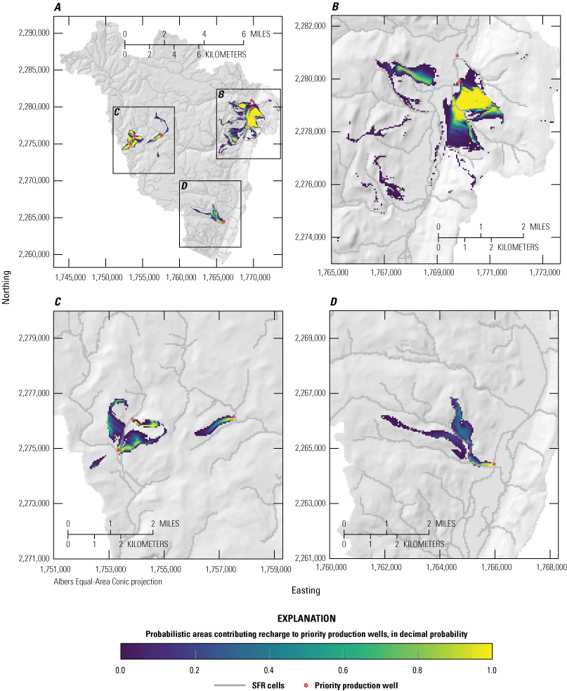
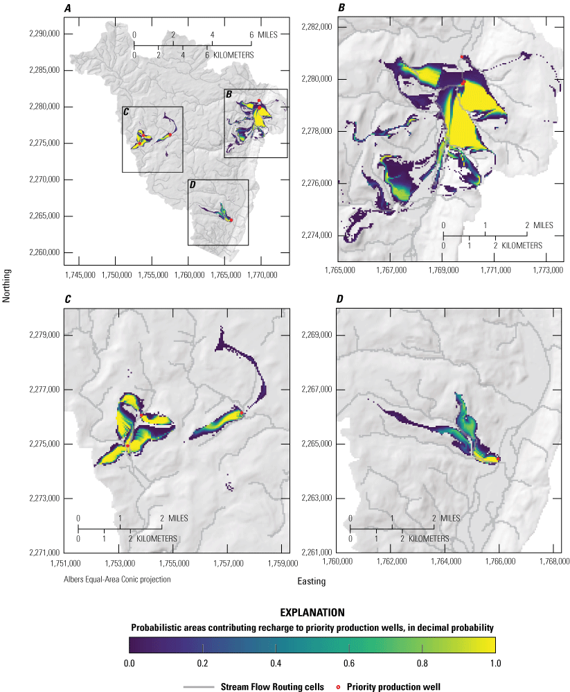
Probabilistic areas contributing recharge to priority wells under the “Baseratio” pumping scenario. Panels show, A, full study area results, B, detail view of priority wells near Ellenville, C, detail view of priority wells near Woodridge and Mountain Dale, and, D, detail view of priority well near Wurtsboro. Colormap is scaled to the probability that a location contributes recharge to priority wells (red circles). A location with a value of 1.0 is within the area contributing recharge to a priority well in 100 percent of simulations. A location with a value of 0.5 is within the area contributing recharge to a priority well in 50 percent of simulations. A location outside of the color flood is within the area contributing recharge to a priority well in 0 percent of simulations.

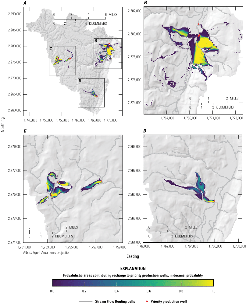
Probabilistic areas contributing recharge to priority wells under the “Maxratio” pumping scenario. Panels show, A, full study area results, B, detail view of priority wells near Ellenville, C, detail view of priority wells near Woodridge and Mountain Dale, and, D, detail view of priority well near Wurtsboro. Colormap is scaled to the probability that a location contributes recharge to priority wells (red circles). A location with a value of 1.0 is within the area contributing recharge to a priority well in 100 percent of simulations. A location with a value of 0.5 is within the area contributing recharge to a priority well in 50 percent of simulations. A location outside of the color flood is within the area contributing recharge to a priority well in 0 percent of simulations.
Probabilistic areas contributing recharge to priority wells under the “0.25ratio” pumping scenario. Panels show, A, full study area results, B, detail view of priority wells near Ellenville, C, detail view of priority wells near Woodridge and Mountain Dale, and, D, detail view of priority well near Wurtsboro. Colormap is scaled to the probability that a location contributes recharge to priority wells (red circles). A location with a value of 1.0 is within the area contributing recharge to a priority well in 100 percent of simulations. A location with a value of 0.5 is within the area contributing recharge to a priority well in 50 percent of simulations. A location outside of the color flood is within the area contributing recharge to a priority well in 0 percent of simulations.
Probabilistic areas contributing recharge to priority wells under the “0.5ratio” pumping scenario. Panels show, A, full study area results, B, detail view of priority wells near Ellenville, C, detail view of priority wells near Woodridge and Mountain Dale, and, D, detail view of priority well near Wurtsboro. Colormap is scaled to the probability that a location contributes recharge to priority wells (red circles). A location with a value of 1.0 is within the area contributing recharge to a priority well in 100 percent of simulations. A location with a value of 0.5 is within the area contributing recharge to a priority well in 50 percent of simulations. A location outside of the color flood is within the area contributing recharge to a priority well in 0 percent of simulations.

Probabilistic areas contributing recharge to priority wells under the “0.75rate” pumping scenario. Panels show, A, full study area results, B, detail view of priority wells near Ellenville, C, detail view of priority wells near Woodridge and Mountain Dale, and, D, detail view of priority well near Wurtsboro. Colormap is scaled to the probability that a location contributes recharge to priority wells (red circles). A location with a value of 1.0 is within the area contributing recharge to a priority well in 100 percent of simulations. A location with a value of 0.5 is within the area contributing recharge to a priority well in 50 percent of simulations. A location outside of the color flood is within the area contributing recharge to a priority well in 0 percent of simulations.
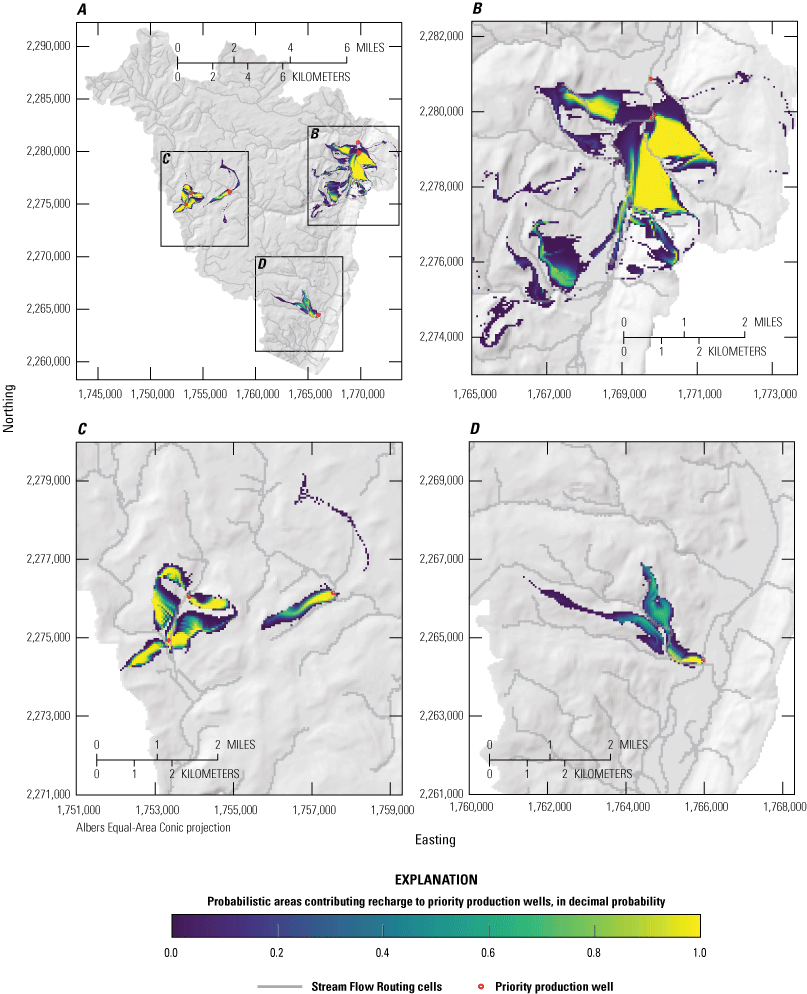
Probabilistic areas contributing recharge to priority wells under the “Maxrange” pumping scenario. Panels show A, full study area results, B, detail view of priority wells near Ellenville, C, detail view of priority wells near Woodridge and Mountain Dale, and, D, detail view of priority well near Wurtsboro. Colormap is scaled to the probability that a location contributes recharge to priority wells (red circles). A location with a value of 1.0 is within the area contributing recharge to a priority well in 100 percent of simulations. A location with a value of 0.5 is within the area contributing recharge to a priority well in 50 percent of simulations. A location outside of the color flood is within the area contributing recharge to a priority well in 0 percent of simulations
Panel B of figures 26–31 shows the probabilistic contributing recharge area to the 4 priority wells near Ellenville, N.Y. The Ellenville contributing recharge area is the largest in size for all scenarios, owing the number (4) and density of wells and their combined maximum withdrawal rates (table 1). The Ellenville footprint extends to the south, to near Spring Glen, N.Y., and the upper Sandburg Creek drainage (fig. 1). The footprint also extends laterally to the east and west up the valley walls into the uplands, particularly to the east of Ellenville between the tributary streams draining Shawangunk Ridge. The highest probability areas of the Ellenville contributing recharge area were typically simulated along the eastern part of the valley floor and the eastern uplands, with some high probability areas also simulated in the western uplands.
Panel C of figures 26–31 shows the probabilistic contributing recharge areas to the 3 priority wells near Woodridge (2) and Mountain Dale (1), N.Y. Contributing recharge areas near the two western wells near Woodridge cover parts of the valley floor near the wells and, to a larger extent, areas in the uplands to the north, east, and west of the wells. The contributing recharge area for the eastern well, pumping from a confined aquifer unit near Mountain Dale, includes an area south of the well in the uplands and a small part of the valley floor near the well. During intermediate and higher pumping scenarios, additional contributing areas are simulated in the uplands to the north and south of the well (fig. 27, for example); however, these areas have relatively low probability of contributing recharge.
Panel D of figures 26–31 shows the probabilistic contributing recharge area to the priority well near Wurtsboro. N.Y. The contributing recharge area for this well includes a part of the valley floor near the well and the uplands to the west of Wurtsboro. The extent of this well’s contributing recharge footprint does not change greatly among pumping scenarios, but results indicate that increased pumping at this well leads to increased probability of recharge contribution.
Each pumping scenario represents an outcome that, when used for planning purposes, corresponds to a different level of risk tolerance; for example, pumping rates in the “Maxratio” scenario are scaled to maximum capacities, creating the largest contributing recharge footprint and large areas of high probability near wells. Management decisions made using results from this scenario (fig. 27) would be relatively risk averse. Alternatively, pumping rates in the “Baseratio” scenario are adjusted only by history matching and remain near 2010–2015 reported mean levels, creating contributing recharge footprints that are relatively small and smaller high probability areas. Management decisions made using “Baseratio” results (fig. 26) would be relatively risk tolerant. Management decisions made using and the intermediate scaled and ranged pumping scenarios (“0.25ratio,” “0.5ratio,” “0.75ratio,” and “Maxrange”) therefore represent intermate levels of risk tolerance. Taken together, these results offer a view of the overall uncertainty of the areas contributing recharge to priority wells in the NS–RO study area and provide a tool for risk-based decision making related to the source water protection of these wells.
Assumptions and Limitations of Analysis
The NS–RO groundwater-flow model is a simplification of an infinitely complex natural system. The model integrates large amounts of information about the groundwater system (including aquifer and stream-network geometries, subsurface hydrologic properties, and measurements of water levels and flow), but there are inevitably areas of the model where information is sparse. Considerable effort was put into quantifying model prediction uncertainty stemming from the uncertain model parameters and observation data, but it is more difficult to quantify uncertainty related to “structural error” (Doherty and Welter, 2010). Structural error can be caused by oversimplification or insufficient information and can limit the model’s ability to accurately represent the natural system; for example, consolidating hydrostratigraphic units into model layers. We attempted to mitigate the effects of structural error by applying a highly parameterized approach to model construction and history matching, using pilot point, zone, and cell multipliers to adjust model properties with as much flexibility as we judged appropriate. Despite these limitations, the model provides a useful framework for investigating broader questions related to the regional flow system and the delineation of areas contributing recharge to priority wells.
Model Discretization
The model discretizes the groundwater-flow system into a simplified model grid, consisting of cells that are 50 m on a side and to more than 100 m in thickness. Values in these model cells therefore represent averages of the respective cell volumes. Similarly, simulated outputs from each cell represent average conditions within that cell.
Steady State Assumption
For the purposes of simulating contributing recharge areas to priority wells it was assumed that the steady state simulations were appropriate. In this model, recharge estimates from 2000 to 2013 overlap with water use estimates developed from the 2010–2015 pumping data. Perfect alignment of stresses and observations with the steady-state period is difficult to obtain which can affect the results. Furthermore, steady state conditions represent a time-averaged delineation of source water areas and can smooth over temporal variability (Rayne and others, 2014). However, the relatively high hydraulic conductivity in the glacial sediments—where the priority wells are screened—likely negates much of the transience that can cause elasticity of the source water areas.
Data Gaps
Observation data used for history matching were few and often of poor or unknown quality. This was especially true for hydraulic head observations, where all but one observation was from NYSDEC well completion reports. Flux observations were developed from BFI estimates, which are also uncertain. We adapted to this by including realizations of observation values consistent with their uncertainty for the history matching effort.
Only two flux calibration targets were available. Furthermore, the flux and hydraulic head datasets did not always overlap in time with the steady-state period. The groundwater-flow model simulated base flow only, so the targets are expected to be representative of the groundwater contribution to flow only. However, the presence of the Neversink Reservoir just upstream from streamgage 01436500 made it difficult to assess the groundwater contribution only. The uncertainty of the reservoir outlet importance at streamgage 01436500 was, in part, incorporated into the weight for that observation. Nonetheless, more streamflow data on this stream and others in the model would better constrain the water balance.
Particle Tracking
At base pumping levels, some of the priority wells represented in the groundwater-flow model are strong sinks and others are weak sinks. Strong sinks extract water from the entire cell depth, whereas weak sink well cells extract water from some of the cell’s depth but also let some water pass through the cell without being extracted (Abrams and others, 2013). Allowing particles to pass through weak sinks in this model could therefore lead to an underprediction of the areas contributing recharge to wells. To avoid underpredicting the size of the contributing recharge areas, the particle tracking analysis in this study stopped all particles when they reached weak sinks. This approach offers a conservative estimate of the areas that contribute recharge to the priority wells but may slightly overpredict the size of and the probability that these areas contribute recharge to the wells.
Each particle tracking Monte Carlo analysis consisted of 384 particle tracking simulations—one for each realization in the posterior parameter ensemble. In this study, it was assumed that the 384 realizations were sufficient to reach statistical stationarity in the probabilistic contributing recharge areas. An evaluation of the effect of ensemble size on contributing recharge area stationarity was completed by Fienen and others (2021). This evaluation indicated that higher probability areas tend to stabilize with fewer realizations than the lower probability areas and that the threshold for contributing recharge area stationarity depends on the user’s adopted level of risk tolerance. The probabilistic contributing recharge areas maps produced by this study (figs. 26–31) are considered generally representative but may slightly underpredict the extent of low probability contributing recharge areas. Use of a larger ensemble for the particle tracking Monte Carlo analysis would likely have resulted in similar probability maps—particularly in high probability areas—but with some additional low-probability areas. Further discussion on the effect of ensemble size to map stationarity is presented in Fienen and others (2021).
Summary
Glacial aquifers are the principal source of water for many communities in upstate New York. The high permeability and the shallow depth to the water table in these aquifers make them highly suspectable to contamination. Protecting these aquifers from contamination is critical in areas where groundwater use is high and alternative sources of drinking water are not readily available. Water managers need accurate information about the size and location of the land surface area that contributes recharge to production wells to make land-use planning decisions to reduce the risk of aquifer contamination.
The New York State Department of Environmental Conservation (NYSDEC) and the New York State Department of Health (NYSDOH) are working to reduce the risk of glacial aquifer contamination by delineating areas that contribute recharge to production wells and to encourage land-use planning within these zones. In southeastern New York, the villages of Ellenville, Wurtsboro, Woodridge, the hamlet of Mountain Dale, and surrounding communities rely on groundwater pumped from shallow valley-fill glacial aquifers for public water supply. In this region, which encompasses adjacent parts of the Neversink River and Rondout Creek drainage basins, the NYSDEC and NYSDOH have designated eight “priority” production wells, for which water supply protection is of primary concern. In 2019, in cooperation with the NYSDEC and the NYSDOH, the U.S. Geological Survey began a study to characterize the regional groundwater-flow system and to delineate the contributing areas for these eight priority wells for the purpose of source water protection.
To complete these objectives, a groundwater-flow model of the valley-fill aquifers in the Neversink-Rondout study area in the Neversink River and Rondout Creek drainage basins was created to simulate the groundwater system and evaluate flow paths to a series of eight priority wells. The MODFLOW 6 groundwater model was built using Python tools (such as flopy, modlfow-setup, and sfrmaker) that facilitate transparent and repeatable model development using existing datasets. The model was calibrated to hydraulic head, base flow, and land surface data with a stepwise estimation of model parameters using an iterative ensemble smoother implementation of the Parameter ESTimation software PEST++ (version 5.0.0). We evaluated prior “best guess” parameter bounds with a prior Monte Carlo analysis. Results of the first prior Monte Carlo analysis were used to make informed adjustments to model parameter bounds (typically resulting in expanded bounds, notably in bedrock hydraulic conductivity), and a second prior Monte Carlo analysis was run to identify improved ranges for model parameters during calibration. We used results of the second Monte Carlo analysis to set parameter bounds and starting values for calibration via history matching using the iterative ensemble smoother.
The history matching effort produced an ensemble of parameter values for the groundwater-flow model that spans the range of values within prior uncertainty bounds and is informed by the historical observation data, within a reasonable range of uncertainty on those observations. This history-matched ensemble was used to delineate the areas contributing recharge to priority wells by running the groundwater-flow and particle tracking (MODPATH7) models both for each ensemble member. Deterministic contributing areas computed for each ensemble member were aggregated to produce maps showing the probability that a location contributes recharge to priority wells. Finally, the particle tracking Monte Carlo analysis was repeated for six pumping scenarios, representing a wide range of possible pumping levels, to incorporate uncertainty in future pumping rates related to population growth or other management decisions. Increasing pumping rates generally led to larger contributing recharge areas and larger areas of high probability that a location contributes recharge to priority wells. These maps show the overall uncertainty of the areas contributing recharge to priority wells in the study area and provide a tool for risk-based decision making for protection of well source water.
References Cited
Abrams, D., Haitjema, H., and Kauffman, L., 2013, On modeling weak sinks in MODPATH: Ground Water, v. 51, no. 4, p. 597–602. [Also available at https://doi.org/10.1111/j.1745-6584.2012.00995.x].
Bakker, M., Post, V., Langevin, C.D., Hughes, J.D., White, J.T., Starn, J.J., and Fienen, M.N., 2016, Scripting MODFLOW model development using Python and flopy: Groundwater, v. 54, i. 5, p. 733-739. [Also available at https://doi.org/10.1111/gwat.12413].
Como, M., 2013, Hydrogeologic appraisal of the unconsolidated aquifer in Wawarsing, New York: Stony Brook, Stony Brook University, M.S. thesis, 36 p., 50 pls., [Also available at https://www.geo.sunysb.edu/reports/MComo_FinalReport.pdf].
Doherty, J., 2003, Ground water model calibration using pilot points and regularization: Ground Water, v. 41, no. 2, p. 170–177. [Also available at https://doi.org/10.1111/j.1745-6584.2003.tb02580.x].
Doherty, J., and Welter, D., 2010, A short exploration of structural noise: Water Resources Research, v. 46, no. 5, W05525. [Also available at https://dx.doi.org/10.1029/2009wr008377].
Feinstein, D.T., Hart, D.J., Gatzke, S., Hunt, R.J., Niswonger, R.G., and Fienen, M.N., 2020, A simple method for simulating groundwater interactions with fens to forecast development effects: Ground Water, v. 58, no. 4, p. 524–534. [Also available at https://doi.org/10.1111/gwat.12931].
Fienen, M.N., and Corson-Dosch, N.T., 2021, Groundwater model archive and workflow for Neversink/Rondout Basin, New York, source water delineation: U.S. Geological Survey data release, at https://doi.org/10.5066/P9HWSOHP.
Fienen, M.N., Corson‐Dosch, N.T., White, J.T., Leaf, A.T., and Hunt, R.J., 2021, Risk‐based wellhead protection decision support: a repeatable workflow approach. Groundwater. [Also available at https://doi.org/10.1111/gwat.13129].
Finkelstein, J.S., Woda, J.C., and Williams, J.H., 2022, Data sources and methods for digital mapping of eight valley-fill aquifer systems in upstate New York: U.S. Geological Survey Scientific Investigations Report 2022–5024, 21 p., https://doi.org/10.3133/sir20225024.
Fischer, J.M., Riva-Murray, K., Hickman, R.E., Chichester, D.C., Brightbill, R.A., Romanok, K.M., and Bilger, M.D., 2004, Water quality in the Delaware River Basin, Pennsylvania, New Jersey, New York, and Delaware, 1998–2001: U.S. Geological Survey Circular 1227, 39 p. [Also available at https://doi.org/10.3133/cir1227].
Langevin, C.D., Hughes, J.D., Banta, E.R., and Niswonger, R.G., Panday, Sorab, and Provost, A.M., 2017, Documentation for the MODFLOW 6 Groundwater Flow Model: U.S. Geological Survey Techniques and Methods, book 6, chap. A55, 197 p. [Also available at https://doi.org/10.3133/tm6A55].
Leaf, A.T., Fienen, M.N., and Reeves, H.W., 2021, SFRmaker and Linesink-maker—Rapid construction of streamflow routing networks from hydrography data: Groundwater. [Also available at https://doi.org/10.1111/gwat.13095].
Miller, T.S., Sherwood, D.A., Jeffers, P.M., and Mueller, N., 1998, Hydrogeology, water quality, and simulation of ground-water flow in a glacial-aquifer system, Cortland County, New York: U.S. Geological Survey Water-Resources Investigations Report 96–4255, 84 p., 5 plates. [Also available at https://doi.org/10.3133/wri964255].
New York State Department of Environmental Conservation, 2020, Water Well Contractor and Completion Report Record Search, accessed July 16, 2020 at, https://www.dec.ny.gov/lands/33317.html.
Pollock, D.W., 2016, User guide for MODPATH Version 7—A particle-tracking model for MODFLOW: U.S. Geological Survey Open-File Report 2016–1086, 35 p. [Also available at https://doi.org/10.3133/ofr20161086].
Randall, A.D., 2001, Hydrogeologic framework of stratified-drift aquifers in the glaciated Northeastern United States: U.S. Geological Survey Professional Paper 1415-B, 190 p. [Also available at https://pubs.usgs.gov/pp/1415b/report.pdf].
Rayne, T.W., Bradbury, K.R., and Zheng, C., 2014, Correct delineation of capture zones using particle tracking under transient conditions: Ground Water, v. 52, no. 3, p. 332–334, https://ngwa.onlinelibrary.wiley.com/doi/10.1111/gwat.12141.
Smith, M.J., and Williams, J.H., 2020, Aquifer Test Locator: U.S. Geological Survey webpage, accessed July 29, 2020, at https://doi.org/10.5066/P9XQL1MZ.
U.S. Geological Survey, 2015, 3-County LiDAR, point data, online at ftp://ftp.gis.ny.gov/elevation/LIDAR/USGS_3County2014/.
U.S. Geological Survey, 2020a, USGS water data for the Nation: U.S. Geological Survey National Water Information System database, accessed July 22, 2020, at https://doi.org/10.5066/F7P55KJN.
U.S. Geological Survey, 2020b, The StreamStats program: U.S. Geological Survey web page, accessed August 17, 2020, at https://streamstats.usgs.gov/ss/.
U.S. Geological Survey, 2018, National Hydrography Dataset (ver. NHDPlus High Resolution Beta for Hydrologic Unit (HU) 4-0202 and 4-0204 (published 20180606)): U.S. Geological Survey web page, accessed September 4, 2020, at https://usgs.maps.arcgis.com/apps/MapTools/index.html?appid=41a5c2ca49bd4a83b239450e61022d53.
Westenbroek, S.M., Kelson, V.A., Dripps, W.R., Hunt, R.J., and Bradbury, K.R., 2010, SWB—A modified Thornthwaite-Mather Soil-Water-Balance code for estimating groundwater recharge: U.S. Geological Survey Techniques and Methods book 6, chap. A31, 60 p. [Also available at https://doi.org/10.3133/tm6A31].
White, J.T., Fienen, M.N., and Doherty, J.E., 2016, A python framework for environmental model uncertainty analysis: Environmental Modelling & Software, v. 85, p. 217–228. [Also available at https://doi.org/10.1016/j.envsoft.2016.08.017].
White, J.T., 2018, A model-independent iterative ensemble smoother for efficient history- matching and uncertainty quantification in very high dimensions: Environmental Modelling & Software, v. 109, p. 191–201. [Also available at https://doi.org/10.1016/j.envsoft.2018.06.009].
White, J.T., Hunt, R.J., Fienen, M.N., and Doherty, J.E., 2021, Approaches to highly parameterized inversion: PEST++ version 5, a software suite for parameter estimation, uncertainty analysis, management optimization and sensitivity analysis: U.S. Geological Survey Techniques and Methods 7-C26, Book 7, Chapter 26. [Also available at https://doi.org/10.3133/tm7C26.]
White, J.T., Foster, L.K., Fienen, M.N., Knowling, M.J., Hemmings, B., and Winterle, J.R., 2020. Toward reproducible environmental modeling for decision support: A worked example: Frontiers in Earth Science, v. 8, article 50, 11 p. [Also available at https://doi.org/10.3389/feart.2020.00050].
Wills, J., Merguerian, C., and Bigolski, J.N., 2005. Post-Alleghenian deformation of the Shawangunk ridge in NY and NJ: Conference proceeding, accessed December 15, 2020, at https://pbisotopes.ess.sunysb.edu/lig/Conferences/abstracts05/abstracts/wills.pdf.
Woda, J.C., Finkelstein, J.S., and Williams, J.H., 2022, Interpolated hydrogeologic framework and digitized datasets for upstate New York study areas: U.S. Geological Survey data release, https://doi.org/10.5066/P96R5K5R.
Yager, R.M., Kauffman, L.J., Buchwald, C.A., Westenbroek, S.M., and Reddy, J.E., 2018, Digital products from a hydrogeologic framework for Quaternary sediments within the glaciated conterminous United States: U.S. Geological Survey data release, accessed June 17, 2020, at https://doi.org/10.5066/F7HH6J8X.
Yager, R.M., Kauffman, L.J., Soller, D.R., Haj, A.E., Heisig, P.M., Buchwald, C.A., Westenbroek, S.M., and Reddy, J.E., 2019, Characterization and occurrence of confined and unconfined aquifers in Quaternary sediments in the glaciated conterminous United States (ver. 1.1, February 2019): U.S. Geological Survey Scientific Investigations Report 2018–5091, 90 p. [Also available at https://doi.org/10.3133/sir20185091].
Zell, W.O., and Sanford, W.E., 2020a, Calibrated simulation of the long‐term average surficial groundwater system and derived spatial distributions of its characteristics for the contiguous United States: Water Resources Research, v. 56, no. 8, p. [Also available at https://doi.org/10.1029/2019WR026724].
Zell, W.O., and Sanford, W.E., 2020b, MODFLOW 6 models used to simulate the long-term average surficial groundwater system for the contiguous United States: U.S. Geological Survey data release, accessed June 2, 2020 at https://doi.org/10.5066/P91LFFN1.
Appendix 1. Data Sources Used to Construct the Neversink-Rondout MODFLOW 6 Groundwater-flow Model
Table 1.1.
Summary of publicly available data sources used to build the Neversink-Rondout groundwater-flow model.[MF6; MODFLOW 6; NWIS, U.S. Geological Survey National Water Information System; SWUDS, U.S. Geological Survey Site-Specific Water-Use Data System; NYSDEC, New York State Department of Environmental Conservation; NHDPlus, National Hydrography Dataset Plus; USGS, U.S. Geological Survey; --, Not applicable]
| Model Component | MF6 packagea | File name(s) | Reference | Notes | Link |
|---|---|---|---|---|---|
| Initial hydraulic conductivity values | NPF | -- | Smith and Williams, 2020; Como, 2013 | Aquifer Test Locator web tool, M.S. Thesis | https://doi.org/10.5066/P9XQL1MZ; https://www.geo.sunysb.edu/reports/MComo_FinalReport.pdf |
| Well pumping rates | WEL | -- | NWIS/SWUDS | -- | https://nwis.waterdata.usgs.gov/nwis/wu |
| Model top elevation | DIS, SFR | top_50m_from_lidar.tif | Finkelstein and others, 2022; Woda and others, 2022 | Derived from Lidar; https://gis.ny.gov/ | https://doi.org/10.5066/P9HWSOHP |
| Layer elevations and thicknesses | DIS | L1_Bottom.tif, L2_Bottom.tif, L3_Bottom___TopOfBedrock.tif | Finkelstein and others, 2022; Woda and others, 2022 | Top of lacustrine, bottom of lacustrine, top of bedrock | https://doi.org/10.5066/P9HWSOHP |
| Initial heads | IC | top_50m_from_lidar.tif | Finkelstein and others, 2022; Woda and others, 2022 | -- | https://doi.org/10.5066/P9HWSOHP |
| Active model domain | DIS | Model_Extent_HUC12.shp | Finkelstein and others, 2022; Woda and others, 2022 | -- | https://doi.org/10.5066/P9HWSOHP |
| Boundary condition constant heads | CHD | 0108_0110_0202_0203_MF6_SS_Unconfined_250, 0204_0206_0209_MF6_SS_Unconfined_250 | Zell and Sanford, 2020 | Parent models; heads file used to build constant head boundaries in valleys | https://water.usgs.gov/GIS/metadata/usgswrd/XML/zell2020_wrr.xml |
| Streamflow routing lines | SFR | NHDPLUS_H_0202_HU4_GDB.gdb, NHDPLUS_H_0204_HU4_GDB.gdb | NHDPlus HR; U.S. Geological Survey, 2018 | NHDLine | https://www.usgs.gov/core-science-systems/ngp/national-hydrography/nhdplus-high-resolution |
| Streamflow routing information | SFR | NHDPlusFlowlineVAA, NHDPlusFlow | https://www.usgs.gov/core-science-systems/ngp/national-hydrography/nhdplus-high-resolution | ||
| Stream inflow rates | SFR | -- | NWIS | USGS stream gage 01436000 | https://doi.org/10.5066/F7P55KJN |
| Recharge | RCH | SWB_Nawqa_mm.tif | Yager and others, 2018 | -- | https://doi.org/10.5066/F7HH6J8X |
| Head and flux observations | OBS | -- | NWIS | -- | https://doi.org/10.5066/F7P55KJN |
| Additional head observations | OBS | -- | NYSDEC | Water Well Contractor and Completion Report Record | https://www.dec.ny.gov/lands/33317.html |
References Cited
Bakker, M., Post, V., Langevin, C.D., Hughes, J.D., White, J.T., Starn, J.J., and Fienen, M.N., 2016, Scripting MODFLOW model development using Python and flopy: Groundwater, v. 54, i. 5, p. 733-739. [Also available at https://doi.org/10.1111/gwat.12413].
Como, M., 2013, Hydrogeologic Appraisal of the Unconsolidated Aquifer in Wawarsing, New York: Stony Brook University, M.S. thesis, 36 p., 50 pls., [Also available at https://www.geo.sunysb.edu/reports/MComo_FinalReport.pdf].
Finkelstein, J.S., Woda, J.C., and Williams, J.H., 2022, Data sources and methods for digital mapping of eight valley-fill aquifer systems in upstate New York: U.S. Geological Survey Scientific Investigations Report 2022–5024, 21 p., https://doi.org/10.3133/sir20225024.
Leaf, A.T., Fienen, M.N., and Reeves, H.W., 2021, SFRmaker and Linesink-maker—Rapid construction of streamflow routing networks from hydrography data: Groundwater. [Also available at https://doi.org/10.1111/gwat.13095].
Smith, M.J., and Williams, J.H., 2020, Aquifer Test Locator: U.S. Geological Survey webpage, accessed July 29, 2020, at https://doi.org/10.5066/P9XQL1MZ.
U.S. Geological Survey, 2018, National Hydrography Dataset (ver. NHDPlus High Resolution Beta for Hydrologic Unit (HU) 4-0202 and 4-0204 (published 20180606)): accessed September 4, 2020, at https://usgs.maps.arcgis.com/apps/MapTools/index.html?appid=41a5c2ca49bd4a83b239450e61022d53.
Woda, J.C., Finkelstein, J.S., and Williams, J.H., 2022, Interpolated hydrogeologic framework and digitized datasets for upstate New York study areas: U.S. Geological Survey data release, https://doi.org/10.5066/P96R5K5R.
Yager, R.M., Kauffman, L.J., Buchwald, C.A., Westenbroek, S.M., and Reddy, J.E., 2018, Digital products from a hydrogeologic framework for Quaternary sediments within the glaciated conterminous United States: U.S. Geological Survey data release, accessed June 17, 2020, at https://doi.org/10.5066/F7HH6J8X.
Zell, W.O., and Sanford, W.E., 2020, MODFLOW 6 models used to simulate the long-term average surficial groundwater system for the contiguous United States: U.S. Geological Survey data release, accessed June 2, 2020 at https://doi.org/10.5066/P91LFFN1.
Conversion Factors
U.S. customary units to International System of Units
International System of Units to U.S. customary units
Datum
Vertical coordinate information is referenced to the North American Vertical Datum of 1988 (NAVD 88).
Horizontal coordinate information is referenced to the North American Datum of 1983 (NAD 83).
Elevation, as used in this report, refers to distance above the vertical datum.
Abbreviations
BFI
base-flow index
CHD
MODFLOW 6 Time-Variant Specified Head Package
HUC
hydrologic unit code
iES
iterative ensemble smoother
Kh
horizontal hydraulic conductivity
Kv
vertical hydraulic conductivity
NS–RO
Neversink-Rondout
NYSDEC
New York State Department of Environmental Conservation
NYSDOH
New York State Department of Health
NWIS
National Water Inventory System
PEST++
Parameter ESTimation Software
SFR
MODFLOW 6 Streamflow Routing Package
USGS
U.S. Geological Survey
Suggested Citation
Corson-Dosch, N.T., Fienen, M.N., Finkelstein, J.S., Leaf, A.T., White, J.T., Woda, J., and Williams, J.H., 2022, Areas contributing recharge to priority wells in valley-fill aquifers in the Neversink River and Rondout Creek drainage basins, New York: U.S. Geological Survey Scientific Investigations Report 2021–5112, 50 p., https://doi.org/10.3133/sir20215112.
ISSN: 2328-0328 (online)
Study Area
| Publication type | Report |
|---|---|
| Publication Subtype | USGS Numbered Series |
| Title | Areas contributing recharge to priority wells in valley-fill aquifers in the Neversink River and Rondout Creek drainage basins, New York |
| Series title | Scientific Investigations Report |
| Series number | 2021-5112 |
| DOI | 10.3133/sir20215112 |
| Year Published | 2022 |
| Language | English |
| Publisher | U.S. Geological Survey |
| Publisher location | Reston, VA |
| Contributing office(s) | New York Water Science Center, Upper Midwest Water Science Center |
| Description | Report: ix, 50 p.; 2 Data Releases |
| Country | United States |
| State | New York |
| Other Geospatial | Neversink River and Rondout Creek Drainage Basins |
| Online Only (Y/N) | Y |
| Additional Online Files (Y/N) | N |
| Google Analytic Metrics | Metrics page |