

Assessment of Well Yield, Dominant Fractures, and Groundwater Recharge in Wake County, North Carolina
Links
- Document: Report (13.1 MB pdf) , HTML , XML
- Data Releases:
- USGS data release - Soil-Water-Balance (SWB) model datasets for the Greater Wake County area, North Carolina, 1981–2019
- USGS data release - National Land Cover Database (NLCD) 2016 products (ver. 2.0, July 2020)
- USGS data release
- USGS data release - Groundwater well yield in Wake County, North Carolina
- Database: USGS National Water Information System database - USGS water data for the Nation
- Version History: Version History (508 B txt)
- Download citation as: RIS | Dublin Core
Acknowledgments
The authors would like to show appreciation for the support of the Wake County Environmental Services during this study. Thanks go to Nancy Daly for assistance in securing site access for several wells for the monitoring network installation and Evan Kane for providing the county well-construction data. Special thanks to Phil Bradley, North Carolina Geological Survey, for his review and supporting geologic data that contributed to a better understanding of the local Piedmont geology.
Abstract
A cooperative study led by the U.S. Geological Survey and Wake County Environmental Services was initiated to characterize the fractured-rock aquifer system and assess the sustainability of groundwater resources in and around Wake County. This report contributes to the development of a comprehensive groundwater budget for the study area, thereby helping to enable resource managers to make sound and sustainable water-supply and water-use decisions.
Construction information was used to analyze the well depth, casing depth, and reported well yield of more than 7,500 inventoried wells. The median well depth and casing depth were 265 feet (ft) below land surface (bls) and 68 ft bls, respectively, and the median well yield was 10 gallons per minute. Generally, well yield increased with depth to around 200 ft bls and then began to decrease with depth within the fractured-rock aquifer.
Borehole geophysical logging methods were used to characterize the fractured-rock aquifer by mapping the orientation of geologic structures within the subsurface. Structure measurements were made on resulting log data and mapped to observed general spatial trends within the regional groundwater system and more distinct hydrogeologic units. Many of the fractures observed within the borehole logs are steeply dipping across Wake County, although open fractures with shallow dip angles were also observed in most rock classes. Regional geologic structural trends were observed in proximity to the Jonesboro Fault.
Potential groundwater recharge in the study area was estimated using a Soil-Water-Balance (SWB) model, as well as using base flow hydrograph separation. The SWB model calculated net infiltration below the root zone for 1981 through 2019 for a 5,402-square-mile area that extends to the counties surrounding Wake County. The mean annual net infiltration rate for the 39-year period was about 8.6 inches per year for the study area. The mean annual net infiltration results from the SWB model were comparable to annual base flow estimates using the PART hydrograph-separation method at six U.S. Geological Survey streamgages within the study area. Mean annual base flow for all six drainage basins was near 7.5 inches per year and estimates ranged from 2.9 to 8.9 inches. Comparisons of mean annual potential recharge from the SWB model and base flow estimates were generally within 2 inches, except during high flows for most of the drainage basins in the study area.
Introduction
Wake County is one of the most populated counties in North Carolina and one of the fastest growing counties in the United States, having a residential population of 1.1 million residents (State of North Carolina, 2020; U.S. Census Bureau, 2020). Roughly 18 percent of Wake County residents depend on groundwater as their primary drinking-water source, withdrawing an estimated 16 million gallons per day (Mgal/d; U.S. Geological Survey, 2015b). The population is projected to double within the next 40 years, which will increase demand for drinking-water resources and place additional stress on the fractured-rock aquifer. With increasing development within Wake County over the next several decades, effects on the groundwater system involve potential changes in recharge and withdrawal rates. During periods of drought, less groundwater may be available for consumptive use. Competition for groundwater resources may induce well interference and reduced well yields at a local scale (Chapman and others, 2011). Change in land use, including increased urbanization, affects stream base flow and groundwater recharge rates (Rose and Peters, 2001; Hardison and others, 2009) by causing an increase in surface runoff and a decrease in infiltration to the groundwater system.
Wake County regulates private wells, a primary drinking water source for most rural residents. State legislation (North Carolina General Assembly, 2003) requires all units of local government and large community water systems that provide public water service to more than 1,000 service connections or more than 3,000 people to prepare a local water supply plan. Wake County supports the development of a water supply plan in accordance with the 50-year planning window used by the North Carolina Division of Water Resources for residents in unincorporated areas of the county. To develop this supply plan, Wake County seeks to better understand the sustainability of groundwater resources of the fractured-rock aquifer system.
Purpose and Scope
This report provides hydrologic information for the local groundwater system that can be used to guide planning and development for Wake County, North Carolina. This report includes (1) a compilation and summary of existing well construction data across Wake County, (2) an establishment of a countywide groundwater monitoring network to observe long-term (annual) water-level trends, (3) a characterization of fracture orientation and density in the local bedrock, and (4) an estimation of net infiltration via precipitation recharge to groundwater.
Study Area
Wake County is in central North Carolina and is predominantly within the Piedmont physiographic province, and a small area (35 square miles [mi2]) in southeastern Wake County is in the Coastal Plain physiographic province (fig. 1). The county spans a total of 857 mi2 and ranges in elevation from 137 to 558 feet (ft) above the North American Vertical Datum of 1988 (NAVD 88). Wake County has a humid subtropical climate with mean temperatures ranging from 47 to 71 degrees Fahrenheit (°F) and receives about 46 inches (in.) of precipitation each year (National Oceanic and Atmospheric Administration, 2020). The Neuse and Cape Fear River Basins make up the two primary river basins within Wake County. The Neuse River Basin covers most of the county and includes major streams such as Crabtree Creek, Walnut Creek, and Middle Creek. The Neuse River Basin also includes several lakes such as Falls Lake in northern Wake County, which serves as the primary drinking-water source for the city of Raleigh, as well as smaller lakes such as Lake Crabtree, Lake Wheeler, and Lake Benson. The southwestern corner of the county lies within the Cape Fear River Basin and includes Harris Lake.
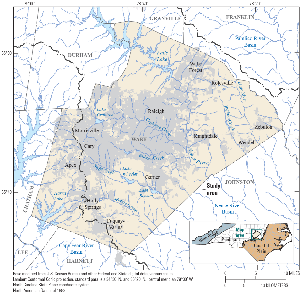
The Wake County study area overlying the Piedmont and Coastal Plain physiographic provinces of North Carolina, including major rivers, major cities, and relevant drainage basins. Color-shaded areas represent city and town limits.
Wake County includes the city of Raleigh, the State capital, and many other municipalities: Cary, Apex, Morrisville, Holly Springs, Fuquay-Varina, Garner, Wake Forest, Rolesville, Knightdale, Wendell, and Zebulon (fig. 1). The population of Wake County exceeds 1 million people (1,085,297; State of North Carolina, 2020), and 35 percent of the county is developed (fig. 2; Dewitz, 2019). Other predominant land cover classes in 2016 include forested land (39 percent), hay/pasture (7 percent), and cultivated crops (5 percent).
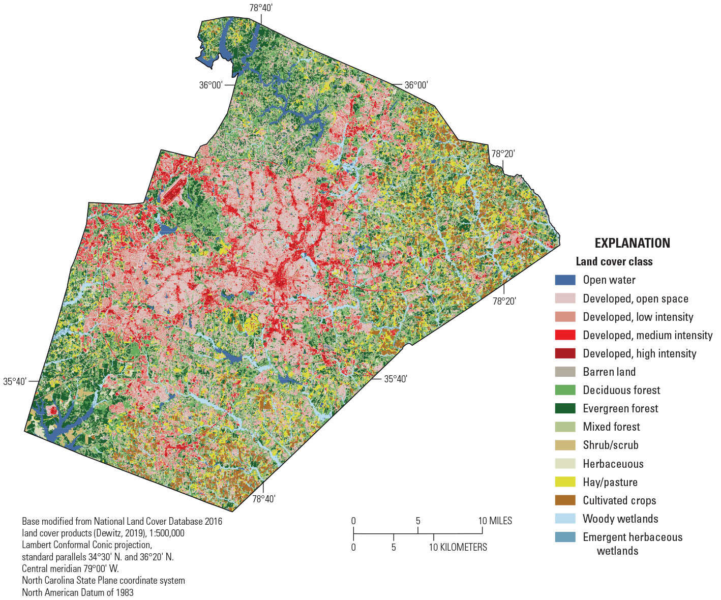
National Land Cover Database 2016 land cover data for Wake County, North Carolina (modified from Dewitz, 2019).
The Piedmont region of North Carolina is primarily underlain by metamorphic and igneous rocks, with sedimentary rocks present in down-faulted Mesozoic basins. Unmetamorphosed igneous intrusive rocks are present as diabase dikes and granitic veins or as batholith-scale intrusions. Rocks within the Piedmont are broken and displaced by faults, shear zones, and stress-relief fractures (joints) that provide conduits through which groundwater can flow. Fractured-rock aquifer systems can be defined by the complex distributions of aquifer properties, where most of the groundwater storage is largely within the overlying regolith, which consists of soil, alluvium, and weathered in-place bedrock (saprolite), that may subsequently flow parallel to the bedrock or downward through a system of faults and joints, foliated and sheared planar features, and fractured bedding planes (Heath, 1984; Daniel and Harned, 1998). A simplified schematic of a fractured-rock aquifer system (fig. 3) illustrates how groundwater flows through a network of fractures. Well placement in the fractured-rock aquifer is especially important because groundwater flow is dependent on the location, depth, and density of permeable fractures with hydrologic connection to groundwater recharge and discharge areas.
The bedrock in the study area can be characterized by five general rock classes: (1) igneous intrusive, (2) metaigneous, (3) metavolcanic, (4) sedimentary, and (5) metasedimentary rocks (table 1). The rock classes are further divided into 15 distinct hydrogeologic units based on mapping work done in the Piedmont and Blue Ridge physiographic provinces of North Carolina by Daniel and Payne (1990) (table 2; fig. 4; Daniel, 1989). The classification of the hydrogeologic units is linked to the water-bearing potential of the rock classes, where composition and texture affect primary porosity and the development of secondary porosity (fractures and solution openings), as well as the rate of weathering. The Triassic sedimentary rocks that fill the Mesozoic basin in the western part of the county are bounded to the east by the north-northeast trending Jonesboro Fault, separating the basin from the hydrogeologic units of the metaigneous and metavolcanic rock types to the east (fig. 4).
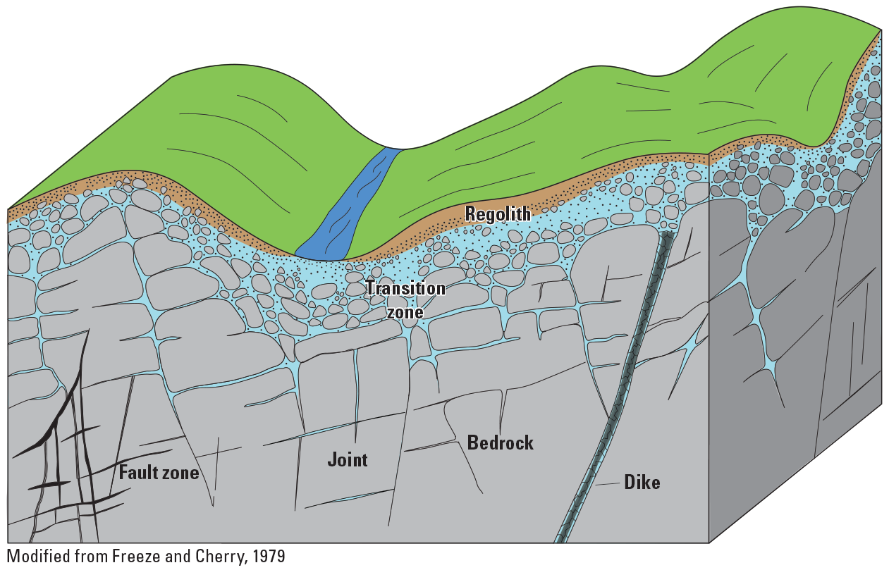
Schematic of generalized fractured-rock aquifer system.
Table 1.
Generalized formation, porosity, and permeability of rock classes in Wake County, North Carolina.[%, percent; m/s, meter per second]
Table 2.
Lithologic description of hydrogeologic units by rock class in Wake County, North Carolina (modified from Daniel, 1989).[mi2, square mile; <, less than]
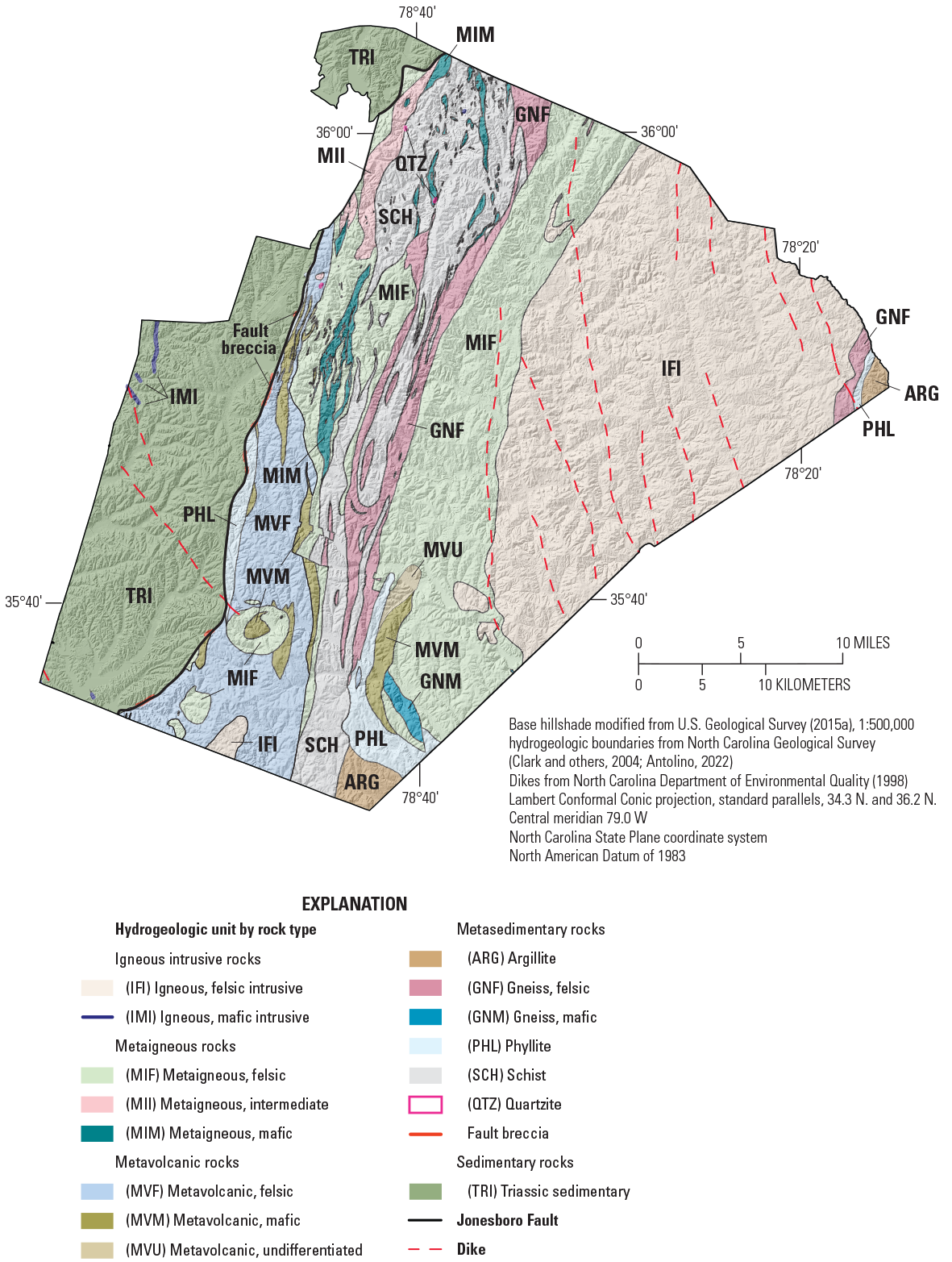
Hydrogeologic units, Jonesboro Fault, and dikes in Wake County, North Carolina. Hydrogeologic unit map based on Daniel (1989), Daniel and Payne (1990), and Clark and others (2004) and available in Antolino (2022).
Previous Investigations
Among the first assessments of groundwater resources in Wake County, May and Thomas (1968) completed a detailed study of groundwater availability, quality, and potential through an analysis of well yields and water-quality samples from domestic, industrial, and municipal wells. Field work was completed between 1961 and 1963, where well-yield information was obtained from well owners and drillers from 268 wells. Water samples were collected for 69 selected wells in the study area. Correlations of well yield were made between rock types and topographic location (hills, flats, slopes, and draws), indicating adequate domestic supply in igneous and metamorphic rocks and generally higher yields for wells within draws, or low areas between hills, than in other topographic areas.
Welby and Wilson (1982) described the relation between certain geological factors such as bedrock type and well yields and examined several other factors that were traditionally thought to control groundwater occurrence in crystalline rock aquifers. Groundwater recharge estimates by Welby and Wilson (1982) were made using streamflow information and were in agreement with those derived from the Thornthwaite and Mather (1957) approach to the water balance. Welby and Wilson (1982) concluded that the spatial variability of groundwater recharge should be accounted for in land-use planning decisions rather than well yields alone and that the effect of increased impervious surface on possible decreases in groundwater recharge can result in local water-supply problems.
A comprehensive investigation of Wake County groundwater resources was completed for Wake County Environmental Services approximately 20 years ago (CDM, 2003). Water-budget components were estimated for 14 surface-water drainage basins. Total estimated groundwater withdrawals for the county were about 14 Mgal/d, including 1.8 Mgal/d around lower Falls Lake. The study concluded with several recommendations to the County, including implementation of a long-term groundwater monitoring network and collection of additional information to help quantify local effects of increased development on groundwater resources.
Chapman and others (2005) completed a 2-year field study at the Lake Wheeler Road research station in Wake County, as part of a larger regional investigation, known as the Piedmont and Mountains Resource Evaluation Program (PMREP; Daniel and Dahlen, 2002), to measure ambient groundwater quality and describe the groundwater-flow system at selected research stations in the Piedmont and Blue Ridge physiographic provinces of North Carolina. The results of the study indicate disconnection and interaction among components of the regolith-fractured bedrock groundwater system. Two primary sets of fractures were generally observed within the bedrock: stress relief fractures that crosscut foliation at low dip angles and steeply dipping fractures that run parallel to the foliation. Vertical hydraulic gradients within the well clusters generally indicate downward groundwater movement in topographic highs and upward movement in discharge areas near streams. Groundwater level fluctuations in the shallow and deep wells were reflected in the surface-water stage data, indicating some degree of connection.
Also part of the PMREP, McSwain and others (2009 and 2013) completed a field study at the Raleigh Hydrogeologic Research Station at the Neuse Resource Recovery Facility to describe the geologic framework, measure groundwater quality, characterize the groundwater-flow system, and describe the groundwater/surface-water interaction in the area. A conceptual hydrogeologic cross section was constructed, which included two previously unmapped, nearly vertical diabase dikes intruding the granite beneath the site. Groundwater within the diabase dike seemed to be hydraulically isolated from the surrounding granite bedrock and regolith. Borehole geophysical logs indicated a correlation between foliation and fracture orientation, and most fractures strike parallel to the foliation. Two sets of water-bearing fractures were observed within the granite bedrock, one set that strikes east-northeast with a shallow dip to the south, and the second strikes northeast and dips moderately to steeply to the northwest.
Chapman and others (2011) investigated several dewatered wells within a 2,000-ft radius of 3 community wells, and more than 30 privately owned wells in northern Wake County from March 2008 through February 2009. Water levels in most wells ranged from 100 to 200 ft below land surface (bls), yet 2 of the 3 community supply wells had even deeper water levels that were 261 ft bls. These results indicated a substantial short-term loss of storage in the fractured-rock aquifer and reduced water availability in wells less than 300 ft in depth. The interpretation of fracture traces derived from borehole geophysical logs and surficial mapping measurements indicated two dominant geologic structure trends striking north to south and N. 65 degrees (°) W. that correlated with groundwater-level distribution patterns.
Methods
This section describes the compilation and statistical analysis of well construction information and groundwater well-yield data, installation of a groundwater monitoring network, borehole geophysical logging within the groundwater network wells, the estimation of base flow via hydrograph-separation analysis, and development of a Soil-Water-Balance (SWB) model for net infiltration estimates.
Well Inventory and Yield Analysis
All available well construction information from State and Federal databases was inventoried for well and casing depth and well yield for more than 7,500 sites. Statistical analysis on yield data from the inventoried wells within Wake County provided information on the relation between well-yield patterns and geologic rock class.
Well Inventory
Wells within a 5-mile (mi) buffer zone surrounding Wake County were included in the inventory. Data were compiled from digital well records from the U.S. Geological Survey (USGS) Groundwater Site Inventory and Wake County Environmental Services databases (U.S. Geological Survey, 2020; Gurley and Antolino, 2021). Well records were primarily derived from construction information placed on the well tag or on a GW–1 form, a State form completed by the well driller at the time of well installation. The GW–1 form includes well location, well depth, casing depth, and well-yield data. Well location information often consisted of a tax parcel number and (or) physical address. For the inventory, well latitude and longitude were estimated for each well based first on the centroid of the tax parcel, if available, and second on physical address location. The well inventory, including select well characteristics, compiled for this study is provided in Gurley and Antolino (2021).
Data from GW–1 forms have some limitations. Measurement precision likely varies based on drilling company practices; for example, some well depth, casing depth, and groundwater well-yield values seemed to be rounded to the nearest interval of 10 (for example, 50, 90, or 100). Moreover, groundwater well yield was typically recorded without any other pump test information, such as pumping rate, length of test, and drawdown data (Welby, 1968), which would better describe productivity of the underlying aquifer. Understanding the limitations of the dataset is important when interpreting statistical results.
Graphical, Spatial, and Statistical Analyses of Well Yield
In this study, the complete well inventory was used for spatial analysis. However, only wells within the Wake County boundary were used for graphical and statistical analyses. Graphical analysis was used to identify the relation of well yield with well depth in Wake County. Well depth data were binned by 100-ft bls depth intervals (that is, median well depth data and yield from each bin were grouped by 100-ft bls intervals) for the graphical analysis.
Well yield in the fractured-rock aquifer is not continuous or gradually changing and clusters of wells (for example, throughout a neighborhood) may have well yields that range substantially. Therefore, a gridded thinning method was used to select the highest yielding well per 2,500-ft grid cell, and that selection was used for spatial interpolation (fig. 5A, B). The “Topo to Raster” tool (ArcGIS, Esri Inc.) was used for interpolation across maximum well yield values in Wake County.
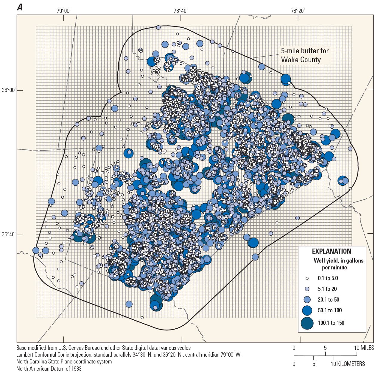

Grid used to thin well-yield data ahead of spatial interpolation, and well-yield data of (A) complete well inventory (number of wells = 7,694) and (B) spatially thinned inventory (number of wells = 2,064).
Statistical analyses were completed to identify the relation between well-yield patterns in Wake County and rock class (table 1, fig. 4). The Wilcoxon rank sum test (Wilcoxon, 1945) was used to test differences in well yield for different rock classes in Wake County: metasedimentary, igneous intrusive, metaigneous, metavolcanic, and sedimentary.
Groundwater Monitoring Network
Between June and October 2019, a monitoring well network was installed across Wake County for the purpose of monitoring water-level trends in the fractured-rock aquifer underlying the study area. The monitoring network consisted of 13 existing monitoring wells and 6 new wells drilled for the purpose of the study. The existing wells included PMREP research station monitoring wells, North Carolina Division of Water Resources continuous monitoring wells, and former domestic supply wells on city and county property. The six newly drilled wells were on property owned by Wake County and the town of Holly Springs. The monitoring network contains 15 wells that are open hole within the bedrock; 4 of these wells are paired with shallow wells that are screened within the regolith (table 3). Continuous water-level measurements were collected at all sites using an internally logging pressure transducer. With the exception of the North Carolina Division of Water Resources wells, water-level data were uploaded via real-time satellite platforms to the USGS National Water Information System (U.S. Geological Survey, 2020) and field verified with manual tapedowns every 6 to 8 weeks.
Table 3.
Well information for groundwater-monitoring network sites. Site numbers and station names were obtained from U.S. Geological Survey (2020).[NAVD 88, North American Vertical Datum of 1988; ft, foot; in., inch; gal/min, gallon per minute; Rd, Road; NC, North Carolina; --, no data or not applicable; RS, Research Station; nr, near; FS, Fire Station; MS, Middle School; Hwy, Highway; Pk, Park; Co, County]
Borehole Geophysical Logging and Imaging
Geophysical logging and imaging were completed in the 15 bedrock monitoring wells (table 3, fig. 6). Logs collected from each well included caliper, electrical resistivity, natural gamma, fluid temperature and specific conductance, optical televiewer, and acoustic televiewer. Characterization of subsurface bedrock structures from geophysical logging included the following: primary lithology, fracture characteristics, foliation (if present), and secondary lithologies and lithologic contacts. Fracture zone characteristics delineated in the 15 wells include depth, dip angle, and dip direction. Fracture zones were delineated at depth in each well using all the borehole logs, including visual delineation from optical and acoustic televiewer images, caliper log diameter increases, resistivity decreases (below the water level), and inflections or slope changes in the fluid temperature and specific conductance logs.
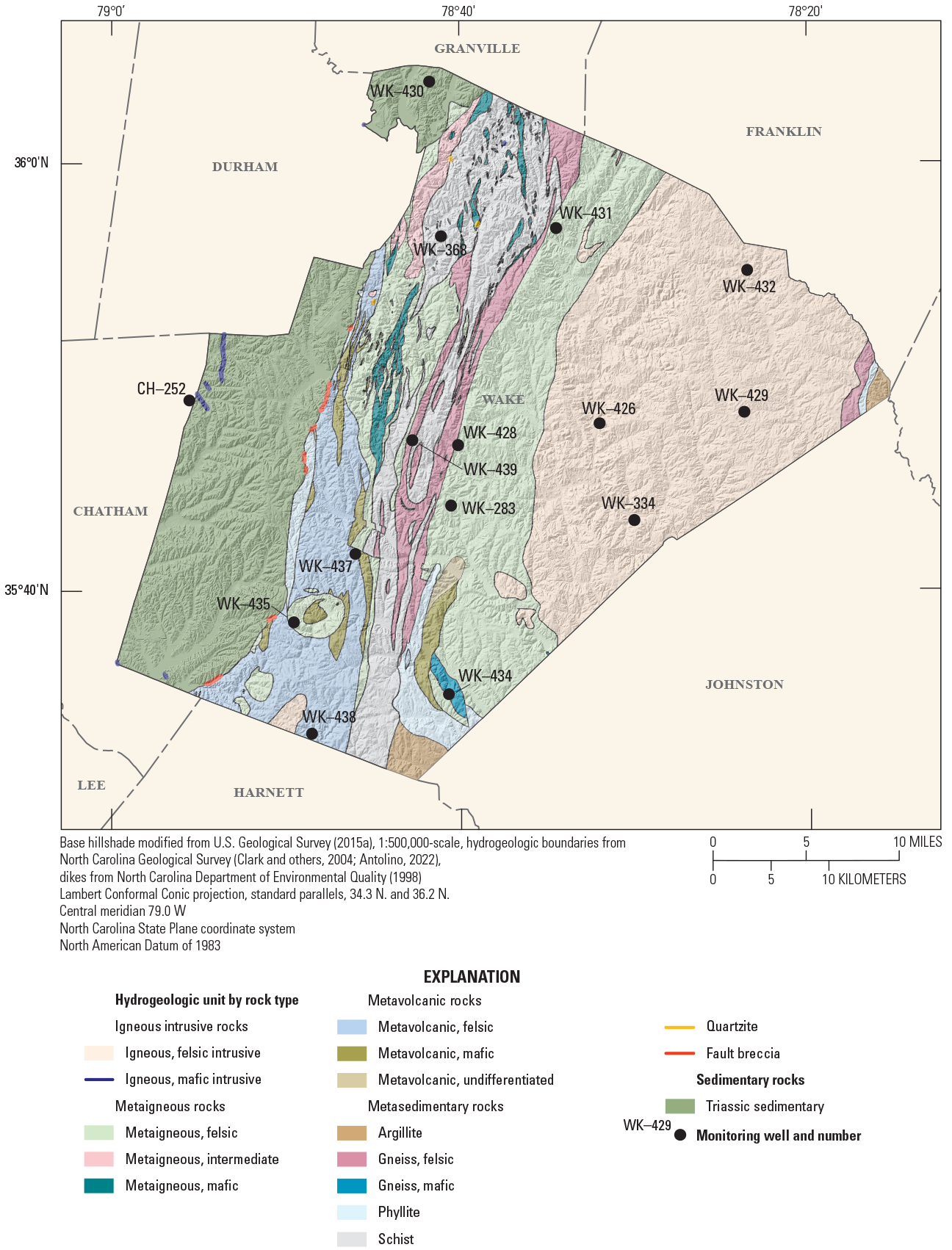
Established groundwater monitoring network wells selected for geophysical logging and imaging.
Continuous and oriented digital color images of the bedrock borehole were recorded from the optical televiewer image logs. The acoustic televiewer image logs show acoustic amplitude and transit time based on an ultrasound pulse-echo system, where lithology and structure changes can be identified regardless of water clarity or visible feature contrast. Both sets of logs are oriented with the use of a magnetometer within the borehole tool and, after accounting for local magnetic declination and borehole deviation, feature orientations can be determined. Interpretations of feature data were based on the optical televiewer and acoustic televiewer image logs using WellCAD software (Advanced Logic Technology, 2021). The orientations were corrected for the measured borehole deviation and a local magnetic declination of 9° west (National Centers for Environmental Information Geomagnetic Modeling Team and British Geological Survey, 2019). WellCad also was used to produce rose diagrams to show delineated fracture orientations. Collected borehole logs are uploaded to the USGS Log Archiver and publicly available via the USGS GeoLog Locator (https://webapps.usgs.gov/GeoLogLocator).
Groundwater Recharge Estimation
Potential groundwater recharge was estimated using base flow hydrograph separation and net infiltration calculation from a SWB model (Westenbroek and others, 2010, 2018). This study assumes that surface-water basins and groundwater basins generally coincide within the study area and that groundwater discharge to streams, or base flow, is nearly equal to groundwater recharge to the fractured-rock aquifer. With these assumptions, base flow estimates from hydrograph separation can be used as groundwater recharge estimates within the streamgage drainage basins. Net infiltration estimates simulated by the SWB model reflects water in the soil column below the plant root zone and is considered to represent potential groundwater recharge in this report. The estimates of potential groundwater recharge from the SWB model were compared and corroborated with the estimates derived from hydrograph separation of streamflow records.
Hydrograph Separation
Hydrograph-separation methods were used to estimate base flow for the 4,067-mi2 total drainage area of 6 of the 12 USGS streamgages within the 15,889-mi2 study area (fig. 7, table 4). The six streamgages selected for analysis were those whose drainage basins were at least 90 percent within the SWB model area. Base flow is the component of streamflow largely sustained by groundwater discharge along the stream reach and is distinct from direct surface runoff. Base flow is a proxy for groundwater discharge into a stream where the groundwater-level in the aquifer is at a higher altitude than the water-level in the stream. Control structures and flow regulation within most of the streams in this urbanized setting likely affect expected, natural base flow signatures. This is particularly apparent at streamgages 02087570 and 02089000 downstream from the Falls Lake reservoir.
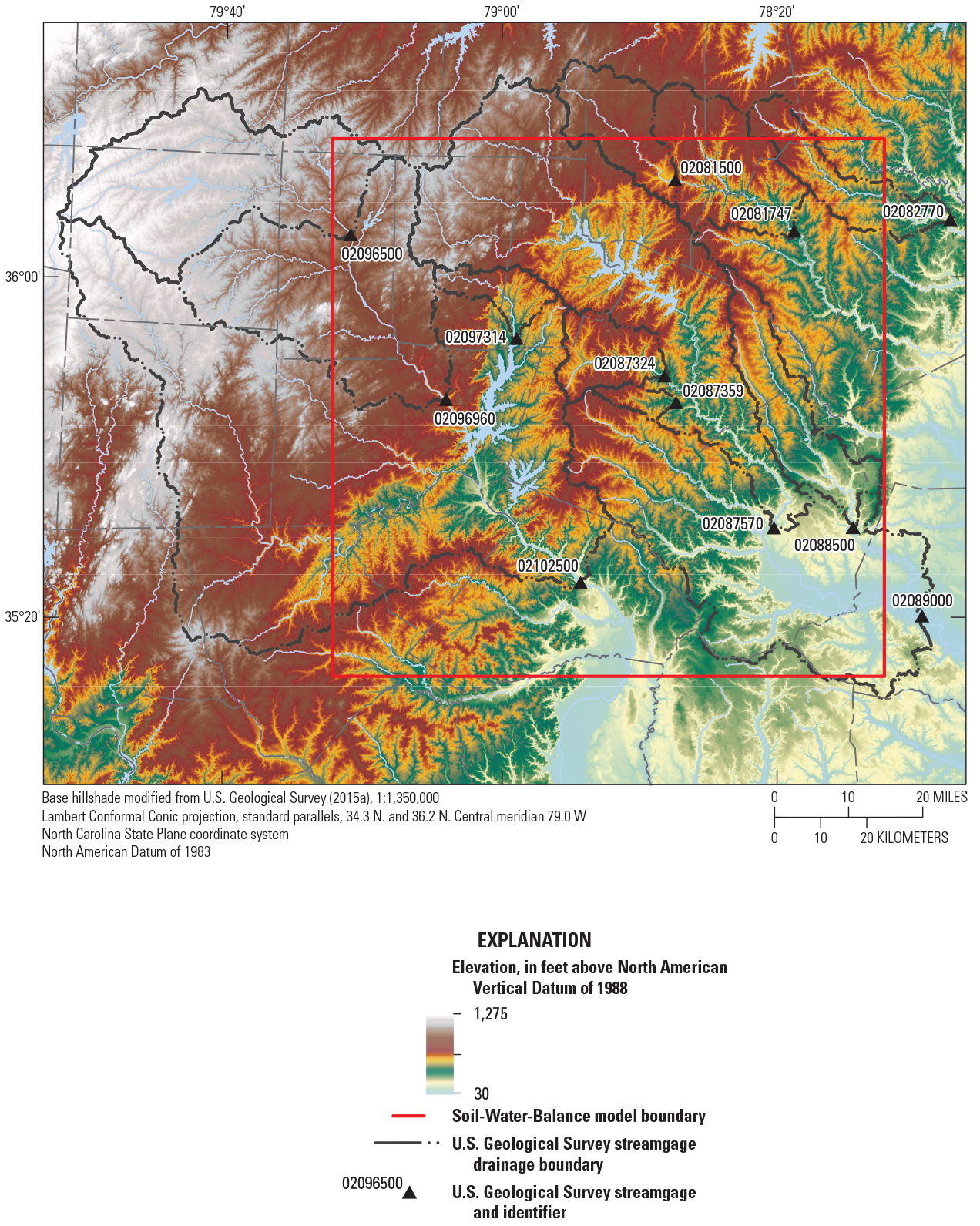
U.S. Geological Survey streamgages and their drainage basins within the Soil-Water-Balance model area.
Table 4.
U.S. Geological Survey streamgages selected for hydrograph estimation analysis.[mi2, square mile; NC, North Carolina; US, U.S.]
Hydrograph separation was performed using the PART method (Rutledge, 1998; Barlow and others, 2015). The PART method designates days that are unaffected by surface runoff as those that are preceded by N days of continuous recession (where N is the total number of days) and linearly interpolates between these days to determine the base flow hydrograph. The period of analysis was January 1980 to December 2019 for all USGS streamgages, dependent on available streamflow record (table 4). The separation method parameters were set to a partition length of N=5 days, a turning point test factor of F=0.90, and a daily recession index of K=0.97915. The limitations and assumptions of applying hydrograph-separation methods in the eastern United States have been described by Nelms and others (2015) and McCoy and others (2015).
Soil-Water-Balance Model
The SWB model 2.0 (Westenbroek and others, 2010, 2018) was used to estimate the distribution of water-budget components in the study area (fig. 7). The SWB model area surrounding Wake County consists of 303,597 grid cells (820-ft spacing) across a 5,402 mi2 study area. The SWB model uses the Soil Conservation Service runoff-curve method (Cronshey and others, 1986) and a modified Thornthwaite-Mather soil-water-balance approach (Thornthwaite, 1948; Thornthwaite and Mather, 1957) to partition precipitation into surface runoff, evapotranspiration (ET), recharge, and water storage in the soil column on a daily time step. The components of the water budget computed by the model rely on the relations among surface runoff, land cover, and hydrologic soil group (Cronshey and others, 1986) and estimated values of ET and temperature (Hargreaves and Samani, 1985). Net infiltration in the SWB model is equal to the surplus water in the soil column below the root zone calculated for each individual cell by its input (precipitation and surface runon) minus the cell output (actual ET, interception, and surface runoff) that is in excess of the maximum soil-water capacity. Surplus water in excess of the maximum recharge rate that is specified in the lookup table for a given soil-land cover combination is considered rejected net infiltration and is passed to downslope cells. SWB modeling does not account for direct infiltration of streamflow loss through streambeds to aquifers or other processes that provide point-source recharge.
The SWB model requires tabular and gridded input datasets that include (1) climate (precipitation and temperature), (2) hydrologic soil group, (3) available soil-water capacity, (4) land cover, (5) surface-water flow direction, and (6) a lookup table with assigned runoff-curve numbers for each land cover class and hydrologic soil group combination. Climatological data included estimates of daily precipitation and daily maximum and minimum temperature in gridded surfaces at a 1-kilometer resolution that were obtained from the Daymet database (Thornton and others, 2016) for the period of 1980 through 2019. Previously published values from Westenbroek and others (2010) were initially used for SWB model parameters in the lookup table and were slightly modified to fit local soil types and wetland vegetation root zone depths.
Soil information on hydrologic soil groups and available water capacity was obtained from the U.S. Department of Agriculture Natural Resources Conservation Service Gridded Soil Survey Geographic Database (Natural Resources Conservation Service, 2020). The four primary hydrologic soil groups, A through D, are defined by ranges of low to high runoff potential, high to low infiltration capacity, and less than 10-percent to greater than 40-percent clay content, respectively (U.S. Department of Agriculture, 2007). The dominant hydrologic soil groups that underlie the study area are B and D at 37 percent and 16.7 percent, respectively (table 5). Dual soil groups, where the water table is within 2 ft of the land surface in groups A, B, and C, make up about 15 percent of the study area. The distribution of hydrologic soil groups within Wake County specifically is similar to the larger SWB area, yet group D soils are the most common soil type at about 28 percent and impervious and open water areas make up nearly 15 percent of the county area compared to only 4.4 percent of the SWB area.
Table 5.
Hydrologic soil groups within the study area based on the Natural Resources Conservation Service Gridded Soil Survey Geographic Database (Natural Resources Conservation Service, 2020).[--, no data]
Land cover datasets were obtained from the National Land Cover Database (Multi-Resolution Land Characteristics Consortium, 2019), and surface water flow direction was derived from a 30-m (98-ft) digital elevation model (U.S. Geological Survey, 2015a). Deciduous, evergreen, and mixed forest land covers about 46 percent of the model area (table 6). Developed land covers 15.7 percent of the study area, and more than one-half consists of developed open space. The digital elevation model was processed to fill all shallow and small closed depressions in the elevation data, which likely reflect artifacts in the data rather than real terrain features, in order to prevent internal drainage.
Table 6.
Land cover within the study area based on the 2016 National Land Cover Database (Multi-Resolution Land Characteristics Consortium, 2019).The SWB model estimates for net infiltration were compared with the annual base flow estimates from the PART hydrograph-separation technique for available years of record between 1981 and 2019 at six USGS streamgages within the model area (table 4). Selected model parameters such as curve numbers, maximum net infiltration, and root-zone depth were manually adjusted to test parameter sensitivity.
Well-Yield Analysis
The well inventory included 7,689 well records; 7,519 wells are within Wake County, and 170 are within 5 mi outside of the county boundary (Gurley and Antolino, 2021). Wells were more prevalent in less-urban areas of the county compared to urban areas and seemed to cluster in some rural neighborhoods. Well depth, casing depth, and well-yield data were skewed right (fig. 8A–C). Well depth ranged from 14 to 975 ft bls (n=7,651, where n is the number of wells). Median well depth was 265 ft bls. Casing depth ranged from 5 to 421 ft bls (n=7,519). Median casing depth was 68 ft bls. Well yield ranged from 0.1 to 150 gallons per minute (gal/min; n=7,689; fig. 8A–C). Median well yield was 10 gal/min.
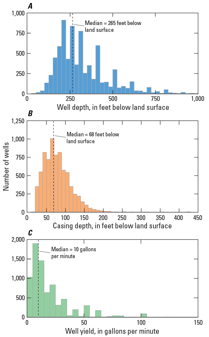
Median of (A) well depth (median = 265 feet below land surface), (B) casing depth (median = 68 feet below land surface), and (C) well yield (median = 10 gallons per minute) in Wake County, North Carolina. [Some count values are too small to be visible on the casing depth and well yield histograms]
The relation between well yield and well depth was typical for a fractured-rock aquifer system in the Piedmont physiographic province of North Carolina; in general, well yield increased with depth to a threshold depth and decreased with depth beyond the threshold (fig. 9). For Wake County, this threshold depth was about 200 ft bls; furthermore, shallower wells in Wake County tended to have greater well yield per foot of total depth, compared to deeper wells.
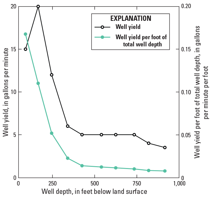
Relation of well yield and well yield per foot of total well depth versus total well depth. The well data were binned by well depth at 100-foot intervals, and median values of depth and yield were graphed for each interval.
Groundwater well yield observed in Wake County was within expectations set from other similar studies that focused on well yield in the Piedmont fractured-rock aquifer. Cunningham and Daniel (2001) determined that well yield in Orange County, N.C. (about 7 mi west of Wake County), ranged from 0.1 to 240 gal/min and had a median of 10 gal/min (n=630). Bailey and others (2018) determined that the Piedmont fractured-rock aquifer in northern Pickens, Greenville, and Spartanburg Counties in South Carolina (not shown) had wells with yields from 0 to 200 gal/min and a median of 8 gal/min (n=1,069).
Predicted maximum expected well yield throughout Wake County based on spatial interpolation of well-yield data is shown in figure 10. Maximum well yield represents the maximum yield expected for new wells drilled. The actual yield for new wells likely falls between zero and the maximum yield value. Maximum well yield varied across Wake County, ranging from 0.1 to 150 gal/min. Lower maximum well yield was measured in the southwestern and northwestern parts of the county concurrent with Triassic sediments. Several pockets of high maximum well yield were in the central, southeastern, and northeastern parts of the county. These patchy patterns of maximum well yield were similar to those detected within the Piedmont aquifers in Orange County, N.C., by Cunningham and Daniel (2001).
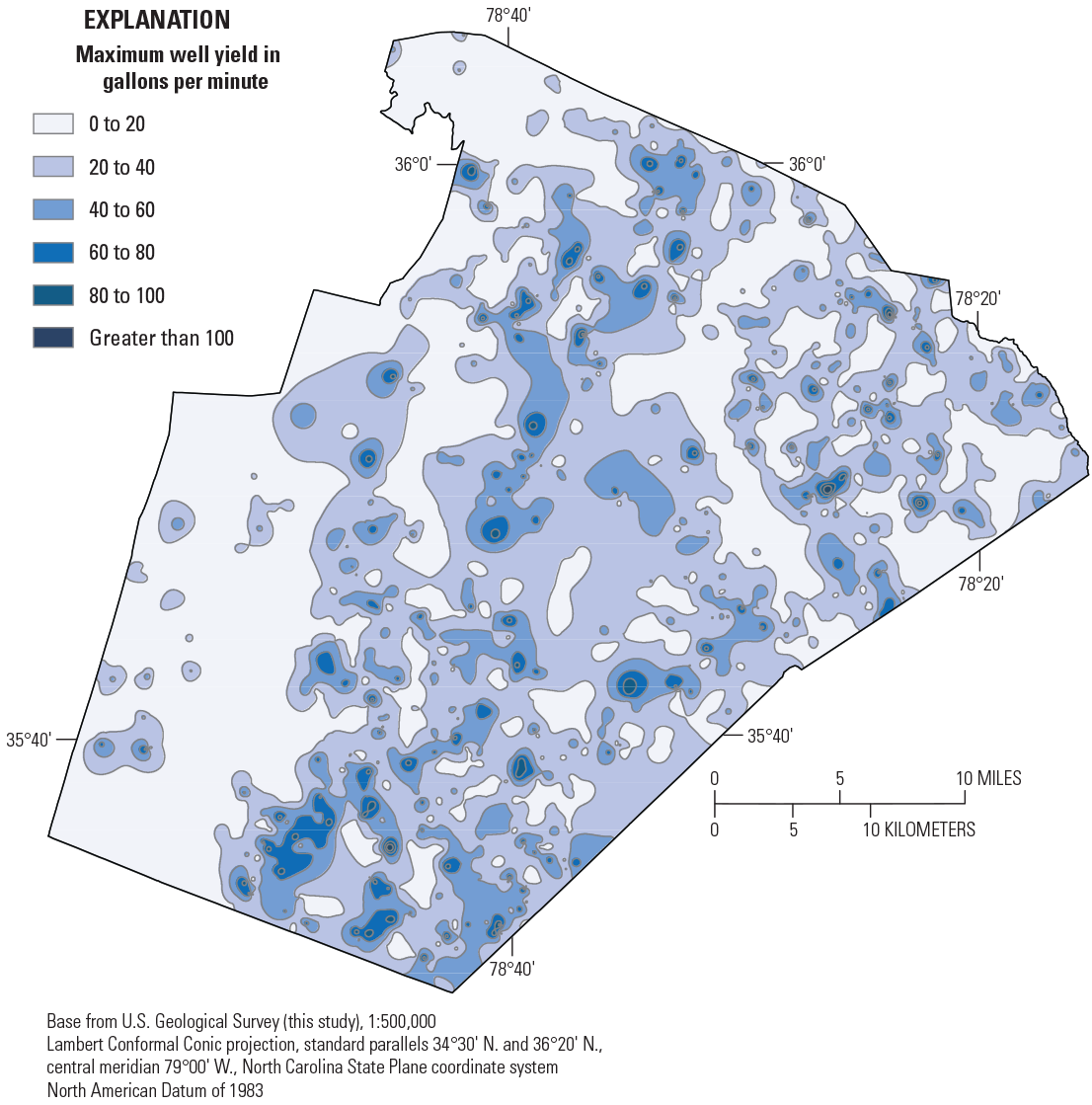
Distribution of maximum well yields in Wake County, North Carolina. Maximum well-yield values indicate that new wells drilled in contoured zones are expected to yield between zero and the contoured zone value.
The Wilcoxon rank sum test revealed statistical differences in well yield based on rock class in Wake County (table 7, fig. 11). A matrix of probability (p-) values from Wilcoxon rank sum test results of well yield by rock class is presented in table 7. The test compares well yield reported from differing rock classes for statistical similarity. Values less than 0.05 were considered significant. Each rock class was compared to each of the other rock classes. The p-values were less than 0.05 for each comparison except for the comparison between metasedimentary and igneous intrusive, which had a p-value of 0.09. The lithologic characteristics and hydrogeologic properties of the rock classes in Wake County support these results (tables 1 and 2).
Table 7.
Matrix of probability values from Wilcoxon rank sum test results of well yield by rock class. The test compares well yield reported from differing rock classes for statistical similarity. Values less than 0.05 were considered significant.[E, denotes exponentiation; --, no data]

Distribution of well yield by rock class (lithology). Differing colors and letter codes represent statistically different datasets.
The highest well yields were measured in the metavolcanic rock class, in southern and central Wake County (figs. 6 and 10). The metavolcanic rock class has more potential for primary and secondary porosity compared with other rock classes in Wake County, and observed interbedding and shearing supports movement of groundwater through the rock (Daniel, 1989; Johnson and others, 201725; Earle, 2019). Together, these features increase the likelihood for this rock class to have higher yields than others in Wake County.
The second highest well yields were measured in the metaigneous rock class, in central Wake County and trending south-southwest to north-northeast (figs. 6 and 10). The metaigneous rock class generally has less primary porosity than metavolcanic rocks but the same potential for secondary porosity resulting from metamorphism. Observed widespread jointing, shearing, and foliation (Daniel, 1989) support movement of groundwater through the rock and support results indicating this rock class as the second-highest yielding in Wake County.
Well yields from igneous intrusive and metasedimentary rock classes in Wake County were not statistically different from each other, although they were different from other rock classes. Well yields from these rock classes were generally lower than well yields from the metavolcanic and metaigneous rock classes and higher than well yields from the sedimentary rock class. With low porosity and no subsequent alteration (that is, metamorphism), groundwater flow through this rock class is likely related to the rocks being predominantly massive with no observed shearing and only some local foliation (table 2). Metasedimentary rocks in Wake County were initially tightly compacted and fine grained, and subsequent metamorphism introduced some foliation that likely supports small amounts of groundwater movement.
The lowest well yields were measured in the sedimentary rock class, in western Wake County (fig. 6). The primary lithology consists of Triassic sediments that were compacted tightly, through which groundwater is not able to flow easily; however, some localized increase in groundwater flow was detected within the Triassic sedimentary rocks near areas intruded by diabase dikes (Bain and Brown, 1981).
Dominant Fracture Orientations
Geophysical logs collected within the monitoring network wells were used to characterize the location and orientation of subsurface features in the fractured-rock aquifer. Fractures were observed in several orientations across all hydrogeologic units in Wake County. The vertical location and spatial distribution of dominant fracture orientations across the county are summarized in this section.
The 15 wells that were used for borehole geophysical logging were within Wake County, with the exception of CH–252, which is just across the Chatham County line (table 3). Well depths ranged from 100 to 601 ft bls. Based on the compilation of casing depths, the inferred regolith thickness ranges from about 21 to 88 ft bls and ranges from 130 to 420 ft above NAVD 88. Groundwater levels measured in all the wells during May–November 2019 ranged from 235.62 ft above NAVD 88 (25.62 ft bls) at WK–426 on May 29, 2019, to 456.80 ft above NAVD 88 (28.37 ft bls) at WK–439 on November 1, 2019. Structures identified within the optical and acoustic televiewer logs were characterized as either primary (open) fractures, secondary (partially open or weathered) fractures, closed or sealed fractures, or foliation. More than 1,400 subsurface structural measurements (orientations) were interpreted from collected optical televiewer and acoustic televiewer images.
Orientations for primary and secondary fractures measured in the 15 wells logged are presented as dip azimuth (dip direction) in rose diagrams shown in figure 12. Fractures exist in several orientations across all hydrogeologic units in Wake County. A list of median structure orientations measured within each rock type and hydrogeologic unit is provided in table 8. Many of the fractures are steeply dipping with median dip angles of primary and secondary fractures ranging from 66 to 89°; however, primary fractures within the igneous intrusive rocks have slightly smaller dip angles. Fractures in the Triassic sedimentary rocks indicate a general eastward dip. Fractures in the metamorphic and igneous rock just to the east of the Jonesboro Fault generally dip to the west. The median dip azimuth for primary and secondary fractures in all metamorphic and igneous rock units is near 221° (southwest) and has a median dip angle near 84°. Where present, measured foliation had a median dip azimuth of 242° (west by southwest) and a dip angle near 84°. The relationship between the median fracture and median foliation dip azimuth provides evidence that many fractures are parallel or subparallel to the foliation, allowing potential groundwater flow where parting exists along foliation planes or schistosity where present. Most of the observed open primary fractures were between 50 and 180 ft bls, and a few open fractures were observed beyond 400 ft bls in metaigneous (WK–283) and metasedimentary (WK–368) rocks (figs. 6 and 13).
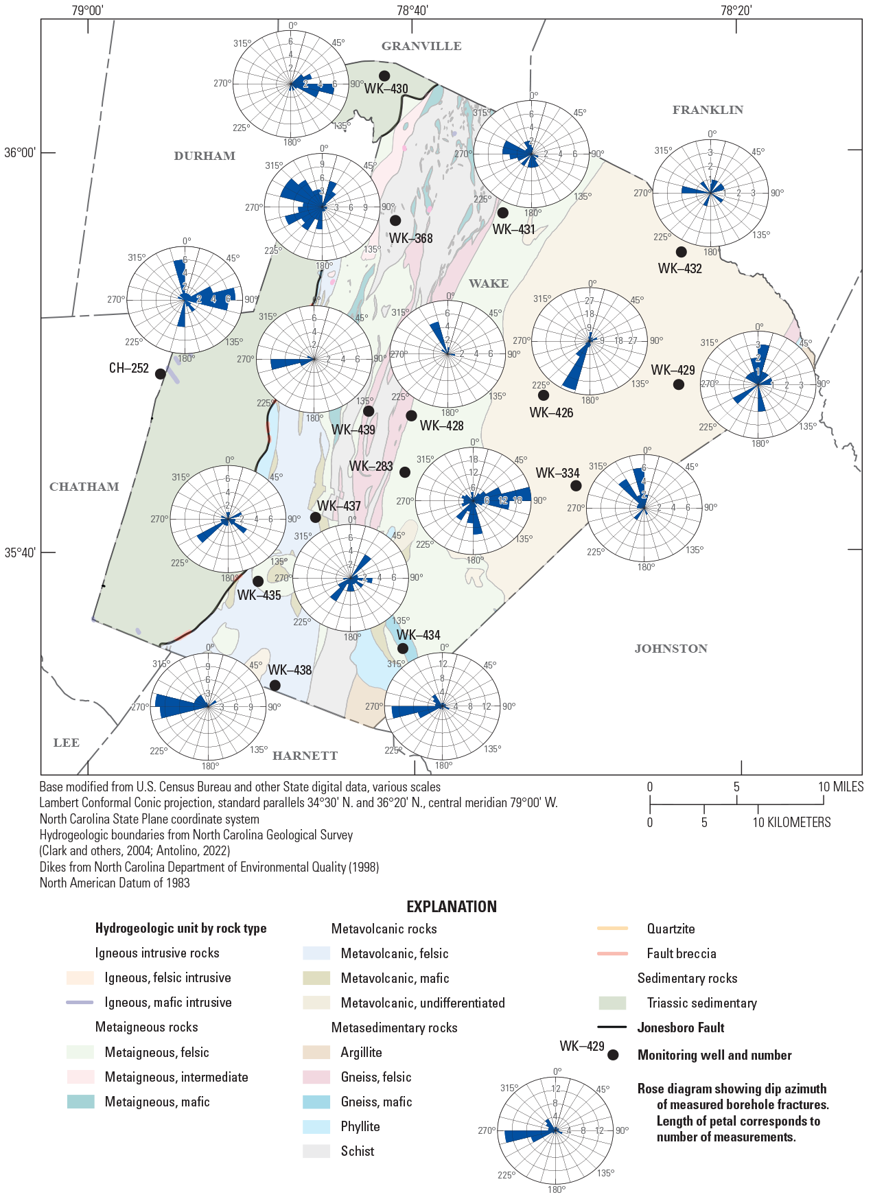
Rose diagrams with dip azimuth of primary and secondary fractures observed from geophysical logs collected in Wake County, North Carolina.
Table 8.
Borehole structure orientations in Wake County, North Carolina, monitoring network wells.[IFI, igneous felsic intrusive; MIF, metaigneous felsic; GNF, gneiss felsic; GNM, gneiss mafic; SCH, schist; MVF, metavolcanic felsic; TRI, Triassic sedimentary]
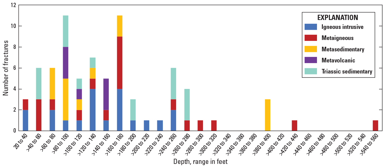
Number of notable primary and secondary fractures by rock class observed in borehole geophysical logs. [>, greater than]
Groundwater Recharge Estimation
Potential recharge to the regional groundwater system was estimated using the PART hydrograph-separation method and an SWB model. Base flow calculated from streamflow records provided an estimate of recharge within each streamgage drainage basin and was compared to the net infiltration of water below the root zone simulated by the SWB model. Model sensitivity was analyzed for the SWB, and the limitations of the modeling method are also discussed. Data generated for groundwater recharge estimation during this study, including the model sensitivity analysis, are available as a USGS data release (Antolino, 2022).
Hydrograph Separation
Variability in annual base flow was estimated from six USGS streamgages using the PART hydrograph-separation technique (table 9) for available records from 1980 to 2019. The mean annual base flow estimates for the six drainage basins ranged from 5.5 (Walnut Creek at Sunnybrook Drive near Raleigh, N.C. [02087359; hereafter referred to as “Walnut Creek”]) to 8.9 in. (Neuse River near Goldsboro, N.C. [02089000]), and the mean base flow for all basins was near 7.5 inches per year (in/yr). Using these mean annual estimates in the six drainage basins, the percentage of streamflow derived from base flow ranged from 33 (02087359) to 65 percent (02089000) of total streamflow. Base flow estimates for all drainage basins were lowest during drought conditions, notably during the 2007–8 and 2011–12 periods, and were generally highest across all basins during the years of 1996 and 2003.
Table 9.
Estimated annual base flow from PART method for six U.S. Geological Survey streamgage drainage basins.[Streamflow refers to streamflow derived from base flow. in., inch; %, percent; --, no data]
Soil-Water-Balance Model
An SWB model run was completed for the 1980–2019 period, which included a model spin-up year that sets up the soil moisture properly for the first year of the desired simulation (1981). Input precipitation values in the climate dataset have an annual mean across the study area of 48.8 in., with mean precipitation ranging from 45.2 to 52.1 in. annually. Input minimum mean daily temperature data ranged from 27 to 49 °F. Input maximum mean daily temperature data ranged from 65 to 87 °F.
The spatial distribution of the mean annual net infiltration estimates from the SWB model for 1981 through 2019 is shown in figure 14. The mean value of the 39-year annual estimates was near 8.6 in/yr for the study area. Estimates were highest for areas with cultivated crop, pasture, grassland, and forest land cover. These land covers make up over two-thirds of the SWB model area and over 50 percent of Wake County (table 6). Developed open space and low-intensity areas underlain by A or B hydrologic soil groups also indicate high amounts of potential groundwater recharge. The lowest estimates were observed in medium to high intensity developed areas, wetland areas, and areas largely underlain by D group soils. The highest potential recharge values were observed on topographic highs and lower values were observed in topographic flats and depressions where groundwater is likely discharging to streams and wetlands. The SWB model calculated annual mean potential recharge rates in excess of 23 in/yr (99th percentile) in isolated areas, notably south of Wake County along the Cape Fear River floodplain and east of Wake County in the Neuse River floodplain. These values are considered anomalous and are likely due to limitations of the SWB model in areas where the water table is close to the surface.

Mean annual net infiltration results from the Soil-Water-Balance model, 1981–2019.
Annual net infiltration estimates were calculated for the six USGS streamgage basins used for base flow estimation (table 10). The New Hope Creek near Blands, N.C. (02097314); Walnut Creek (02087359); and Crabtree Creek at U.S. 1 at Raleigh, N.C. (02087324), streamgage drainage basins have the lowest net infiltration among the six study area basins. These three basins are the smallest of the six, each with an area of less than 130 mi2 (table 4), that also have the highest surface runoff estimates (table 10). Low- to high-intensity development makes up nearly one-half of the land cover within the Walnut Creek drainage basin, reflected in the highest surface runoff estimates across all basins. The lowest net infiltration estimates were observed in the 02097314 drainage basin, where nearly one-half of the basin area is underlain by poorly draining group D or dual soil groups (table 5). The highest net infiltration estimates were observed in the Little River near Princeton, N.C. (02088500), drainage basin, which is the least developed basin with less than 4-percent low- to high-intensity developed land cover.
Table 10.
Annual statistics for outputs from the Soil-Water-Balance model, 1981–2019, for six streamgage basins.[in/yr, inch per year]
In addition to producing estimates of net infiltration below the root zone, the SWB model calculated other important components of the water balance such as actual evaporation and surface runoff. Calculated actual evaporation estimates ranged from 25.3 to 43.0 in/yr, the mean was near 35.4 in/yr within the six USGS streamgage drainage basins, and the mean calculated reference ET was near 27.2 in/yr using the Hargreaves-Samani method (Hargreaves and Samani, 1985; table 10). Annual surface runoff ranged from 5.3 to 30.9 in. per drainage area for the six basins (table 10).
The modeled net infiltration values from the SWB were compared to the estimated base flow values from the six streamgage drainage basins. Annual residuals were computed for 1981 through 2019 by taking the difference between the SWB net infiltration value and the PART base flow estimate. The residuals were squared and summed for each drainage basin to determine the sum of square errors, and then the standard error was computed for each drainage basin based on equation 1.
whereSE
is the standard error,
SSE
is the sum of square errors, and
п
is the number of years of available record used in the PART hydrograph-separation analysis.
When compared with the PART annual base flow estimates, the initial comparisons indicated that SWB annual net infiltration estimates are somewhat variable with standard error values ranging from 1.5 (02087324) to 2.8 in. (02087570 and 02089000). The SWB model generally underestimated higher base flows seen predominantly in the larger drainage basins (fig. 15). Residual values ranged from 4 to −4 in., and values were more positive where base flows exceed 13 in/yr. Of the six drainage basins analyzed, the SWB model, on mean, overestimated base flow for the 02087359 and 02088500 basins, whereas base flow was generally estimated within 2 in. in the other four basins, except during high flows.
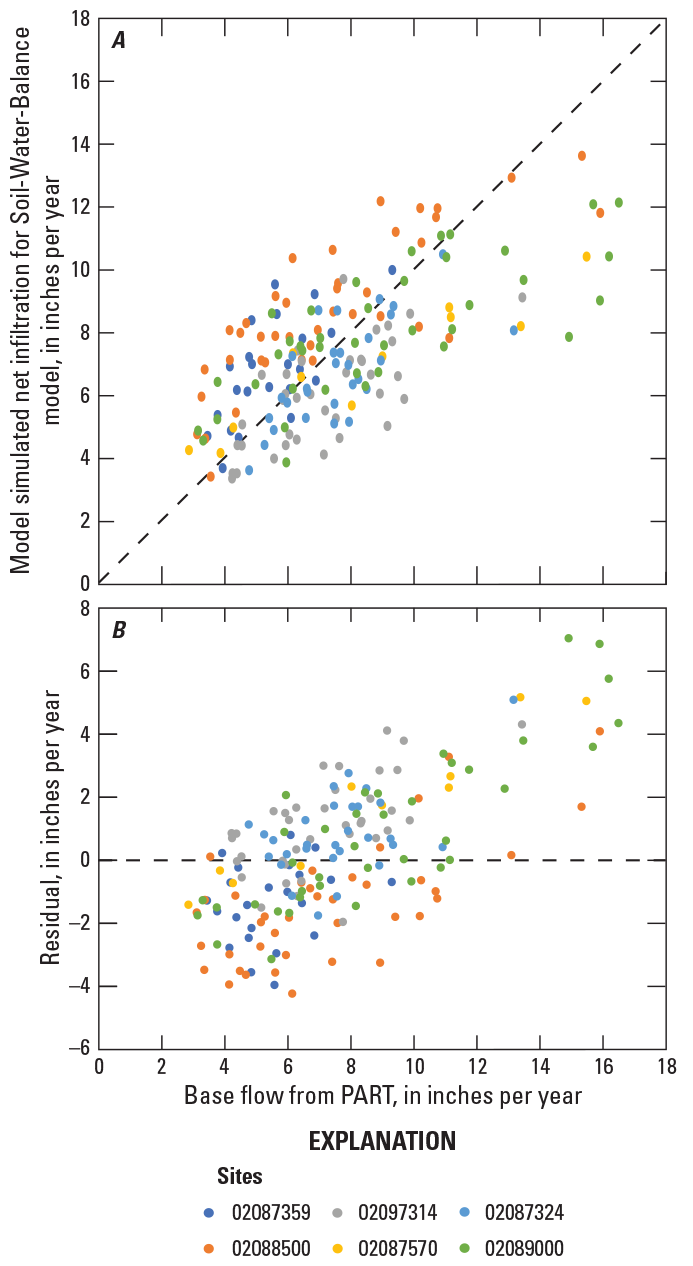
Annual base flow from the PART hydrograph-separation approach compared to Soil-Water-Balance model simulated net infiltration for the calibration drainage basins: (A) 1:1 plots and (B) residuals of model simulated net infiltration, where positive residuals reflect where values were underpredicted by the Soil-Water-Balance model.
Model Sensitivity Analysis
A sensitivity analysis was done to determine general error potential in net infiltration estimates related to uncertainties associated with SWB model lookup table parameters, namely for the curve number, maximum net infiltration rate, and root zone depth. For the sensitivity analysis, the curve number (a value that indicates surface runoff potential), maximum daily net infiltration rate (limit of surplus water below root zone to be considered for net infiltration), and root-zone depth parameters were altered independently for six scenarios: increasing and decreasing the curve number by 10, multiplying the maximum net infiltration rate by a factor of 0.5 and 1.5, and increasing and decreasing the root-zone depth by 1 ft. The sensitivity analysis was run on the representative period of 2002–7 (with 2001 being included as an initial model spin-up year) that contains precipitation values near the historic mean for the study area, encompassing wet and dry years. All land cover and hydrologic soil groups were used for the parameter sensitivity analysis.
The model was most sensitive to changes in maximum net infiltration rate and least sensitive to changes in root zone depth (table 11). Within the basins analyzed, the 02088500 basin was the most sensitive to model parameter uncertainty and the 02087359 basin was relatively the least sensitive. The marked difference in pasture, cropland, and wetland land cover in the 02088500 basin area may explain some of the parameter sensitivity within the basin when compared to the other basins, notably with increased curve numbers. More robust sensitivity analysis using PEST parameter-estimation software (Doherty, 2004) should be considered for future study to better determine nonuniqueness in lookup table parameters, as well as sensitivity to uncertainty in climate input data. Additional measurements of recharge rates determined from aquifer tests and groundwater age tracers at observation wells may also provide better refinement of SWB model parameters.
Table 11.
Standard errors for sensitivity analysis of six scenarios for the Soil-Water-Balance model net infiltration estimates compared with estimated base flows by drainage basin for the period of 2002–7.[--, no data]
| Scenario | Site number | |||||
|---|---|---|---|---|---|---|
| 02087359 | 02088500 | 02097314 | 02087570 | 02087324 | 02089000 | |
| Standard error (inches) | ||||||
| Initial conditions (modified from Westenbroek and others, 2010) | 1.8 | 2.8 | 2.2 | -- | 1.0 | 2.2 |
| Curve number, add 10 | 1.2 | 2.4 | 3.0 | -- | 1.6 | 3.4 |
| Curve number, subtract 10 | 2.0 | 3.6 | 2.1 | -- | 1.0 | 2.4 |
| Root-zone depth, add 1 foot | 1.6 | 2.6 | 2.3 | -- | 1.1 | 2.2 |
| Root-zone depth, subtract 1 foot | 2.0 | 3.0 | 2.0 | -- | 0.9 | 2.3 |
| Maximum daily net infiltration rate, factor of 1.5 | 2.2 | 4.1 | 1.8 | -- | 1.2 | 2.7 |
| Maximum daily net infiltration rate, factor of 0.5 | 1.2 | 1.7 | 4.0 | -- | 2.3 | 3.0 |
Model Limitations
The SWB model includes assumptions and limitations that may influence the interpretation of these results. The application of the runoff-curve numbers to model surface runoff in the SWB is best limited to drainage basin scale rather than parcel or grid-cell scale because the model only captures some variability in runoff-curve numbers due to changes in precipitation, as it has been suggested that the curve number itself may vary by storm event (Hjelmfelt, 1991; Westenbroek and others, 2010). The SWB model is best suited for conditions where the water table is below the plant root zone. The SWB model can be expected to perform poorly in areas where the water table is near or at the land surface, such as wetlands or springs, as the SWB model does not account for rejected infiltration resulting from soil saturation apart from the specification of maximum recharge rate (Westenbroek and others, 2010).
Furthermore, the difference between the SWB and PART estimates may reflect spatial variability in soil properties that is not represented by the SWB within the study area. Uncertainty in the input data (soil properties, land cover, and climate data) because of interpolation or other estimation techniques to handle missing data is also not considered in this analysis. Finally, the differences between the SWB model and PART analysis may indicate that other hydrologic properties or processes are not explicitly accounted for while using the PART method, such as regulated streamflow and effluent discharge, or large groundwater withdrawals.
Summary
This report summarizes findings from the initial phase of the larger assessment of groundwater resources in Wake County, North Carolina, and provides hydrologic information needed to better understand the local groundwater system. Information from well construction, well yields, and fracture orientation was related to geologic rock classes and hydrogeologic units. Spatial and temporal estimates of groundwater recharge were obtained using a Soil-Water-Balance (SWB) model, providing an essential component of the groundwater budget. The recharge estimates were compared to base flow estimates derived from PART hydrograph separation.
Out of more than 7,500 wells inventoried in and around Wake County, the median well depth and casing depth were 265 feet (ft) below land surface (bls) and 68 ft bls, respectively. Well yield ranged from 0.1 to 150 gallons per minute with a median well yield of 10 gallons per minute. Generally, well yield increased with depth to around 200 ft bls and then began to decrease with depth in the fractured bedrock; furthermore, shallower wells in Wake County tend to have greater well yield per foot of total depth, compared to deeper wells. Lower maximum well yield was measured in the southwestern and northwestern parts of the county concurrent with Triassic sedimentary rocks. Higher maximum well yield trended from south-southwest to north-northeast in central Wake County with several pockets of high maximum well yield in the northeastern part of the county. The highest well yields were measured within the metavolcanic rock class, which is known to have more potential for primary and secondary porosity from interbedding and shearing. The lowest well yields were within the sedimentary rock class, which is made up of tightly compacted and cemented Triassic sediments in western Wake County with only localized high yields near diabase dikes. Statistically significant differences in well yields were identified between all the rock classes except for the igneous intrusive and metasedimentary rock classes.
Regional geologic structural trends were observed within the borehole geophysical log data with fractures east of the Jonesboro Fault generally striking north-northeast and dipping to the west and fractures within the Triassic sedimentary rocks generally striking north and dipping to the east. Most of the observed open primary fractures and partially open secondary fractures were between 50 and 180 ft bls, which aligns with the observed high well-yield threshold of 200 ft at depth. Steep and shallow dip angles were observed in subsurface structures captured in the borehole logs across Wake County in most rock classes, yet the median dip angles of primary and secondary fractures ranged from 66 to 89 degrees (°). Where present, measured orientation of foliation within the rock units had a median dip azimuth of 242° and a dip angle near 84°. The structural orientations of primary and secondary fractures indicate nearly the same general trend, providing evidence that many fractures are parallel or subparallel to the foliation, allowing potential groundwater flow where parting exists along foliation planes or schistosity when present.
Recharge to the fractured-rock aquifer underlying Wake County was computed for 1980 through 2019 using the PART hydrograph separation at six streamgages and the SWB model. Annual base flow estimates ranged from 5.5 to 8.9 inches, and the mean base flow for all basins was near 7.5 inches per year. The mean annual estimates for base flow represent a range of 33 to 65 percent of total streamflow within the six drainage basins. Base flow estimates were lowest during drought conditions, notably during the 2007–8 and 2011–12 periods, and were generally highest across all basins during the years of 1996 and 2003. The 39-year mean net infiltration estimate from the SWB model was near 8.6 inches per year for the study area. Comparisons of mean annual potential recharge from the SWB model and base flow estimates were generally within 2 in., except during high flows for most of the drainage basins in the study area. The SWB modeled values generally underestimated base flow in flashy streams during years of heavy rainfall from storm events. The SWB model output indicates net infiltration to the groundwater system is highest in cropland, pasture, and forested areas, as well as open developed areas, although highly variable depending on soil drainage. The lowest and least variable rates of recharge for the period of simulation were computed for developed areas overlying poorly drained soil groups and Triassic sedimentary rock.
References Cited
Advanced Logic Technology, 2021, WellCad: Advanced Logic Technology web page, accessed March 2, 2021, at https://www.alt.lu/products-wellcad/.
Antolino, D.J., 2022, Soil-Water-Balance (SWB) model datasets for the Greater Wake County area, North Carolina, 1981–2019: U.S. Geological Survey data release, https://doi.org/10.5066/P95XKK5V.
Bailey, B., Dripps, W., and Muthukrishnan, S., 2018, Spatial analysis of hydrological productivity in fractured bedrock terrains of the Piedmont of northwestern South Carolina: Journal of South Carolina Water Resources, v. 5, no. 1, p. 25–33. [Also available at https://doi.org/10.34068/JSCWR.05.02.]
Bain, G.L., and Brown, C.E., 1981, Evaluation of the Durham Triassic Basin of North Carolina and technique used to characterize its waste-storage potential: U.S. Geological Survey Open-File Report 80–1295, 138 p., 1 pl. [Also available at https://doi.org/10.3133/ofr801295.]
Barlow, P.M., Cunningham, W.L., Zhai, T., and Gray, M., 2015; U.S. Geological Survey Groundwater Toolbox, a graphical and mapping interface of hydrologic data (version 1.0)—User guide for estimation of base flow, runoff, and groundwater recharge from streamflow data: U.S. Geological Survey Techniques and Methods, book 3, chap. B10, 27 p., accessed August 2020 at https://doi.org/10.3133/tm3B10.
CDM, 2003, Wake County comprehensive groundwater investigation: CDM, 147 p., accessed October 8, 2020, at https://s3.us-west-2.amazonaws.com/wakegov.com.if-us-west-2/prod/documents/2020-10/06%20L5%20-%20WakeCountyCGIFinalReport_web.pdf.
Chapman, M.J., Almanaseer, N., McClenney, B., and Hinton, N., 2011, Fluctuations in groundwater levels related to regional and local withdrawals in the fractured-bedrock groundwater system in northern Wake County, North Carolina, March 2008–February 2009: U.S. Geological Survey Scientific Investigations Report 2010–5219, 60 p. [Also available at https://doi.org/10.3133/sir20105219.]
Chapman, M.J., Bolich, R.E., and Huffman, B.A., 2005, Hydrogeologic setting, ground-water flow, and ground-water quality at the Lake Wheeler Road research station, 2001–03—North Carolina Piedmont and Mountains Resource Evaluation Program: U.S. Geological Survey Scientific Investigations Report 2005–5166, 85 p. [Also available at https://doi.org/10.3133/sir20055166.]
Clark, T.W., Blake, D.E., Stoddard, E.F., Carpenter, P.A., III, and Carpenter, R.H., 2004, Preliminary bedrock geologic map of the Raleigh 30’ x 60’ quadrangle, North Carolina: North Carolina Geological Survey Open-file Report 2004-02, scale 1:100,000, in color. [Also available at https://deq.nc.gov/energy-mineral-and-land-resources/geological-survey/ofrs-geological-survey/ncgs-ofr-2004-02-raleigh-100k-bedrock-geopdf/download.]
Cronshey, R., McCuen, R.H., Miller, N., Rawls, W., Robbins, S., and Woodward, D., 1986, Urban hydrology for small watersheds (2d ed., June 1986): U.S. Department of Agriculture Technical Release 55, 164 p., accessed July 2020 at https://www.nrcs.usda.gov/Internet/FSE_DOCUMENTS/stelprdb1044171.pdf.
Cunningham, W.L., and Daniel, C.C., III, 2001, Investigation of ground-water availability and quality in Orange County, North Carolina: U.S. Geological Survey Water-Resources Investigations Report 2000–4286, 59 p. [Also available at https://doi.org/10.3133/wri004286.]
Daniel, C.C., III, 1989, Statistical analysis relating well yield to construction practices and siting of wells in the Piedmont and Blue Ridge Provinces of North Carolina: U.S. Geological Survey Water-Supply Paper 2341–A, 27 p. [Also available at https://doi.org/10.3133/wsp2341A.]
Daniel, C.C., III, and Dahlen, P.R., 2002, Preliminary hydrogeologic assessment and study plan for a regional ground-water resource investigation of the Blue Ridge and Piedmont Provinces of North Carolina: U.S. Geological Survey Water-Resources Investigations Report 2002–4105, 60 p. [Also available at https://doi.org/10.3133/wri024105.]
Daniel, C.C., III, and Harned, D.A., 1998, Ground-water recharge to and storage in the regolith-fractured crystalline rock aquifer system, Guilford County, North Carolina: U.S. Geological Survey Water-Resources Investigations Report 97–4140, 65 p., accessed August 27, 2020, at https://doi.org/10.3133/wri974140.
Daniel, C.C., III, and Payne, R.A., 1990, Hydrogeologic unit map of the Piedmont and Blue Ridge Provinces of North Carolina: U.S. Geological Survey Water Resources Investigations Report 90–4035, 1 pl. [Also available at https://doi.org/10.3133/wri904035.]
Dewitz, J., 2019, National Land Cover Database (NLCD) 2016 products (ver. 2.0, July 2020): U.S. Geological Survey data release, accessed July 2020 at https://doi.org/10.5066/P96HHBIE.
Doherty, J.E., 2004, PEST—Model-independent parameter estimation user manual 5th ed.: Brisbane, Australia, Watermark Numerical Computing. [Also available at https://www.nrc.gov/docs/ML0923/ML092360221.pdf.]
Earle, S., 2019, Physical geology (2d ed.): Victoria, B.C., Canada, BCcampus, p. 456–457, accessed March 4, 2022, at https://opentextbc.ca/physicalgeology2ed/.
Gurley, L.N., and Antolino, D.J., 2021, Groundwater well yield in Wake County, North Carolina: U.S. Geological Survey data release, accessed July 2021 at https://doi.org/10.5066/P9C2J23X.
Hardison, E.C., O’Driscoll, M.A., DeLoatch, J.P., Howard, R.J., and Brinson, M.M., 2009, Urban land use, channel incision, and water table decline along coastal plain streams, North Carolina: Journal of the American Water Resources Association, v. 45, no. 4, p. 1032–1046. [Also available at https://doi.org/10.1111/j.1752-1688.2009.00345.x.]
Hargreaves, G.H., and Samani, Z.A., 1985, Reference crop evapotranspiration from temperature: Applied Engineering in Agriculture, v. 1, no. 2, p. 96–99. [Also available at https://doi.org/10.13031/2013.26773.]
Heath, R.C., 1984, Ground-water regions of the United States: U.S. Geological Survey Water-Supply Paper 2242, 78 p., accessed August 27, 2020, at https://doi.org/10.3133/wsp2242.
Hjelmfelt, A.T., Jr., 1991, Investigation of curve number procedure: Journal of Hydraulic Engineering, American Society of Civil Engineers, v. 117, no. 6, p. 725–737. [Also available at https://doi.org/10.1061/(ASCE)0733-9429(1991)117:6(725).
Johnson, C., Affolter, M.D., Inkenbrandt, P., and Mosher, C., 2017, An introduction to geology: Salt Lake City, Utah, Salt Lake Community College, accessed March 4, 2022, at https://opengeology.org/textbook/.
May, V.J., and Thomas, J.D., 1968, Geology and ground-water resources in the Raleigh area, North Carolina: North Carolina Department of Water and Air Resources Bulletin no. 15, 147 p. [Also available at https://digital.ncdcr.gov/digital/collection/p16062coll9/id/543723.]
McCoy, K.J., Yager, R.M., Nelms, D.L., Ladd, D.E., Monti, J., Jr., and Kozar, M.D., 2015, Hydrologic budget and conditions of Permian, Pennsylvanian, and Mississippian aquifers in the Appalachian Plateaus physiographic province (ver. 1.1, October 2015): U.S. Geological Survey Scientific Investigations Report 2015–5106, 77 p., accessed March 12, 2019, at https://doi.org/10.3133/sir20155106.
McSwain, K.B., Bolich, R.E., and Chapman, M.J., 2013, Hydrogeology, groundwater seepage, nitrate distribution, and flux at the Raleigh hydrologic research station, Wake County, North Carolina, 2005–2007: U.S. Geological Survey Scientific Investigations Report 2013–5041, 54 p., accessed May 2019 at https://doi.org/10.3133/sir20135041.
McSwain, K.B., Bolich, R.E., Chapman, M.J., and Huffman, B.A., 2009, Water-resources data and hydrogeologic setting at the Raleigh hydrogeologic research station, Wake County, North Carolina, 2005–2007: U.S. Geological Survey Open-File Report 2008–1377, 48 p., accessed May 2019 at https://doi.org/10.3133/ofr20081377.
Multi-Resolution Land Characteristics Consortium, 2019, NLCD 2016 Land Cover (CONUS): Multi-Resolution Land Characteristics Consortium digital data, accessed August 18, 2020, at https://www.mrlc.gov/data?f%5B0%5D=category%3Aland%20cover&f%5B1%5D=region%3Aconus.
National Centers for Environmental Information Geomagnetic Modeling Team and British Geological Survey, 2019, World Magnetic Model 2020: National Oceanic and Atmospheric Administration, National Centers for Environmental Information web page, accessed January 15, 2020, at https://doi.org/10.25921/11v3-da71.
National Oceanic and Atmospheric Administration, 2020, Climate at a glance—County time series: National Oceanic and Atmospheric Administration digital data, accessed September 16, 2020, at https://www.ncdc.noaa.gov/cag/.
Natural Resources Conservation Service, 2020, Gridded Soil Survey Geographic Database (gSSURGO) by State: Natural Resources Conservation Service digital data, accessed August 18, 2020, at https://websoilsurvey.sc.egov.usda.gov/App/WebSoilSurvey.aspx/.
Nelms, D.L., Messinger, T., and McCoy, K.J., 2015, Annual and average estimates of water-budget components based on hydrograph separation and PRISM precipitation for gaged basins in the Appalachian Plateaus Region, 1900–2011: U.S. Geological Survey Data Series 944, 10 p., accessed August 15, 2020, at https://doi.org/10.3133/ds944.
North Carolina General Assembly, 2003, §143–355—Powers and duties of the Department: North Carolina General Assembly, 6 p. [Also available at https://www.ncleg.gov/enactedlegislation/statutes/pdf/bysection/chapter_143/gs_143-355.pdf.]
Rose, S., and Peters, N.E., 2001, Effects of urbanization on streamflow in the Atlanta area (Georgia, USA)—A comparative hydrological approach: Hydrological Processes, v. 15, no. 8, p. 1441–1457. [Also available at https://doi.org/10.1002/hyp.218.]
Rutledge, A.T., 1998, Computer programs for describing the recession of ground-water discharge and for estimating mean ground-water recharge and discharge from streamflow records—Update: U.S. Geological Survey Water-Resources Investigations Report 98–4148, 43 p., accessed June 4, 2018, at https://doi.org/10.3133/wri984148. [Supersedes USGS Water-Resources Investigations Report 93–4121.]
State of North Carolina, 2020, Estimates of the total population of North Carolina counties, and municipalities within counties for July 1, 2019, in July 1, 2020, boundaries: State of North Carolina digital data, accessed October 2020 at https://files.nc.gov/ncosbm/demog/Municipal_Certified_AlphabyCounty_2019.html.
Thornthwaite, C.W., 1948, An approach toward a rational classification of climate: Geographical Review, v. 38, no. 1, p. 55–94. [Also available at https://doi.org/10.2307/210739.]
Thornton, P.E., Thornton, M.M., Mayer, B.W., Wei, Y., Devarakonda, R., Vose, R.S., and Cook, R.B., 2016, Daymet—Daily surface weather data on a 1-km grid for North America, version 3: Oak Ridge, Tenn., Oak Ridge National Library Distributed Active Archive Center for Biogeochemical Dynamics web page, accessed August 8, 2020, at https://doi.org/10.3334/ORNLDAAC/1328.
U.S. Census Bureau, 2020, Quick facts for Wake County, North Carolina: U.S. Census Bureau digital data, accessed December 1, 2020, at https://www.census.gov/quickfacts/wakecountynorthcarolina.
U.S. Department of Agriculture, 2007, Hydrologic soil groups, chap. 7 of National Engineering Handbook: U.S. Department of Agriculture, part 630, accessed October 13, 2020, [Also available at https://www.nrcs.usda.gov/wps/portal/nrcs/detailfull/national/water/?cid=stelprdb1043063.]
U.S. Geological Survey, 2015a, 1/3 arc-second DEM, 3DEP National Elevation Dataset: U.S. Geological Survey digital data, accessed August 18, 2020, at https://viewer.nationalmap.gov/basic/.
U.S. Geological Survey, 2015b, Water use data for North Carolina (2015), in USGS water data for the Nation: U.S. Geological Survey National Water Information System database, accessed July 2020 at https://doi.org/10.5066/F7P55KJN. [State information directly accessible at https://waterdata.usgs.gov/nc/nwis/water_use?wu_year=2015&wu_area=County&wu_county=183&submitted_form=introduction&wu_county_nms=Wake+County.]
U.S. Geological Survey, 2020, USGS groundwater data for the Nation, in USGS water data for the Nation: U.S. Geological Survey National Water Information System database, accessed January 2020 at https://doi.org/10.5066/F7P55KJN. [Groundwater data directly accessible at https://waterdata.usgs.gov/nwis/gw.]
Westenbroek, S.M., Engott, J.A., Kelson, V.A., and Hunt, R.J., 2018, SWB version 2.0—A soil-water-balance code for estimating net infiltration and other water-budget components: U.S. Geological Survey Techniques and Methods, book 6, chap. A59, 118 p., accessed July 2019 at https://doi.org/10.3133/tm6A59.
Westenbroek, S.M., Kelson, V.A., Dripps, W.R., Hunt, R.J., and Bradbury, K.R., 2010, SWB—A modified Thornthwaite-Mather Soil-Water-Balance code for estimating groundwater recharge: U.S. Geological Survey Techniques and Methods, book 6, chap. A31, 60 p. [Also available at https://doi.org/10.3133/tm6A31.]
Wilcoxon, F., 1945, Individual comparisons by ranking methods: Biometrics Bulletin, v. 1, no. 6, p. 80–83. [Also available at https://doi.org/10.2307/3001968.]
Conversion Factors
U.S. customary units to International System of Units
Temperature in degrees Fahrenheit (°F) may be converted to degrees Celsius (°C) as follows:
°C = (°F – 32) / 1.8.
Datum
Vertical coordinate information is referenced to the North American Vertical Datum of 1988 (NAVD 88).
Horizontal coordinate information is referenced to the North American Datum of 1983 (NAD 83) North Carolina State Plane coordinate system.
Altitude, as used in this report, refers to distance above the vertical datum.
For more information about this publication, contact:
Director, South Atlantic Water Science Center
U.S. Geological Survey
1770 Corporate Drive
Norcross, GA 30093
678–924–6700
For additional information, visit: https://www.usgs.gov/centers/sawsc
Publishing support provided by the
Reston and Rolla Publishing Service Centers
Suggested Citation
Antolino, D.J., and Gurley, L.N., 2022, Assessment of well yield, dominant fractures, and groundwater recharge in Wake County, North Carolina (ver. 1.1, May 2022) : U.S. Geological Survey Scientific Investigations Report 2022–5041, 35 p., https://doi.org/10.3133/sir20225041.
ISSN: 2328-0328 (online)
Study Area
| Publication type | Report |
|---|---|
| Publication Subtype | USGS Numbered Series |
| Title | Assessment of well yield, dominant fractures, and groundwater recharge in Wake County, North Carolina |
| Series title | Scientific Investigations Report |
| Series number | 2022-5041 |
| DOI | 10.3133/sir20225041 |
| Edition | Version 1.1: May 2022; Version 1.0: April 2022 |
| Year Published | 2022 |
| Language | English |
| Publisher | U.S. Geological Survey |
| Publisher location | Reston, VA |
| Contributing office(s) | South Atlantic Water Science Center |
| Description | Report: viii, 35 p.; 3 Data Releases; Database |
| Country | United States |
| State | North Carolina |
| County | Wake County |
| Online Only (Y/N) | Y |
| Additional Online Files (Y/N) | N |
| Google Analytic Metrics | Metrics page |