

Simulation of Flow and Eutrophication in the Central Salem River, New Jersey
Links
- Document: Report (12.6 MB pdf) , HTML , XML
- Data Release: USGS data release - WASP model used to simulate flow and eutrophication in the central Salem River, New Jersey
- Download citation as: RIS | Dublin Core
Acknowledgments
The authors thank the U.S. Geological Survey (USGS) staff members who participated in the collection of data for this study, including sampling (Ronald Baker, Timothy Wilson), flow/stage measurement (Robert Schopp, Walter Jones), and surveying (Richard Walker). The authors thank Woodstown Wastewater-Treatment Plant (Craig Loper) and DuPont Chambers Works (Cynthia McManus) employees for providing discharge and diversion data, respectively. The authors thank U.S. Environmental Protection Agency (Tim Wool) and USGS (Ana Garcia) for guidance on water-quality modeling. The authors thank USGS colleagues (Jeffrey Fischer, Mary Chepiga, Susan Colarullo) for comments on report content and organization and New Jersey Department of Environmental Protection (NJDEP) staff members (Helen Pang, Patricia Ingelido) for regulatory guidance. The authors thank USGS colleagues Timothy Wilson and Annett Sullivan; USGS technical specialists (Heather Heckathorn, Thomas Suro); and NJDEP staff for technical review of the report. The authors also thank USGS colleague Martha Watt for assistance with preparation of the model archive data release. Finally, the authors thank the USGS West Trenton Publishing Service Center for editorial review and drafting of the report.
Abstract
The central Salem River in New Jersey is subject to periods of water-quality impairment, marked by elevated concentrations of phosphorus and chlorophyll-a, and low concentrations of and large diurnal swings in concentrations of dissolved oxygen. These seasonal eutrophic conditions are controlling factors for water quality in lower reaches, where the river is more lacustrine than in upper reaches, as a result of downstream damming. This biological productivity is supported by nutrient wash-off from agricultural areas in the surrounding watershed. To investigate this impairment, flow measurement and water-quality sampling were conducted during 2007–08 in support of development of a one-dimensional surface-water-quality model that simulates nutrient cycling and transformation processes.
The U.S. Geological Survey, in cooperation with the New Jersey Department of Environmental Protection, used the U.S. Environmental Protection Agency Water Quality Analysis Simulation Program (WASP) to develop a receiving-water-quality model of the central Salem River between Woodstown and Deepwater, New Jersey, from April 2007 to October 2008. The main-stem river and largest tributary were simulated. In the flow model, kinematic wave flow is used to simulate flow in upper reaches and ponded weir flow is used to simulate flow in lower reaches. The water-quality model makes use of a mass-balance equation to simulate the fate and transport of nutrients, phytoplankton chlorophyll-a, dissolved oxygen, and oxygen demands (an indicator rather than a substance) in the river. Model input included channel characteristics, boundary conditions for flow and water quality, environmental parameters, vertical dispersion coefficients, settling rates, and kinetic constants. Inputs were estimated where field data were lacking, notably for tributary flows and nutrient loads.
The model was calibrated to observed flow variables and concentrations of dissolved oxygen, chlorophyll-a, and nutrients at sampling locations, with emphasis on growing-season conditions. Calibration was achieved through graphical and statistical comparison of simulated results to observed data. Sensitivity analyses were performed, and model limitations and applicability were evaluated. Simulated results closely matched observed data in most cases, although some were overpredicted slightly. The most important causes of overprediction were estimated tributary flows for the flow model and estimated tributary watershed loads for the water-quality model. Calibration of dissolved-oxygen concentrations was closer, and predicted diurnal variations were consistent with high algal photosynthesis/respiration, although lack of continuous dissolved-oxygen data precluded verifying these predictions. A similar caveat applies to predicted diurnal variations in chlorophyll-a. Simulated limitations on algal growth were consistent with those based on observed data and indicated phosphorus was the main limiting nutrient, except during certain periods when nitrogen was limiting.
Two water-quality management scenarios were simulated with the model to assess the effect of point- and nonpoint-source nutrient reductions on water-quality conditions in the river. Scenarios involved (1) a return of watershed land use to predevelopment natural conditions and (2) an extreme reduction in nutrient input. Although the extreme-nutrient-reduction scenario yielded improvements in water quality, the natural-conditions scenario yielded the largest improvements as indicated by minimal violations of surface-water-quality standards or thresholds. However, years may be needed to attain the full benefit of these management scenarios as a result of accumulation of phosphorus and organic carbon in riverbed sediments in lacustrine reaches. The results of this study indicate that the quality of water in the central Salem River will improve if management policies that mitigate the effects of nutrient-loading practices in the watershed, particularly those related to agriculture, are implemented.
Introduction
Development of total maximum daily loads (TMDLs) for impaired surface-water bodies is mandated by the U.S. Environmental Protection Agency (EPA) under the Clean Water Act of 1972. Load equals concentration multiplied by flow. A TMDL is a calculation of the maximum amount of a pollutant a water body can receive and still meet applicable surface-water-quality standards necessary to maintain its chemical, physical, and biological integrity (U.S. Environmental Protection Agency, 1995). A TMDL is a mechanism for identifying all the contributors to surface-water-quality effects and setting goals for reducing loads of pollutants of concern. TMDLs are developed on the basis of the flow and transport-carrying characteristics specific to an impaired water body and are implemented by individual states, in association with EPA. In the central Salem River Basin, the New Jersey Department of Environmental Protection (NJDEP) has identified the Salem River (fig. 1) as an impaired water body, mainly with respect to phosphorus, because the river does not meet Clean Water Act requirements for designated uses resulting from eutrophication caused by elevated nutrient loading (New Jersey Department of Environmental Protection, 2009a, p. B–35). Moderate to severe benthic macroinvertebrate impairment also occurs in the river (New Jersey Department of Environmental Protection, 2010). The trophic state of a water body is controlled largely by flow conditions (for example, depth, volume, tributary inflow), nutrient loads from point and nonpoint sources, and environmental conditions (for example, sunlight, air temperature). The term “nutrients” in this report refers to nitrogen and phosphorus constituents, including dissolved inorganic phosphorus (DIP), dissolved organic phosphorus (DOP), total phosphorus (TP), ammonia (NH4), nitrite plus nitrate (NO2 + NO3), dissolved organic nitrogen (DON), and total nitrogen (TN). Total ammonia includes ammonium ion (NH4) and unionized ammonia (NH3). According to Ji (2008, p. 255), “NH4 concentration is normally much higher than NH3 concentration.” This is why NH4 is sometimes used to represent total ammonia in discussions. This convention is adopted in this report. Also, NO3 was assumed to equal measured total nitrite plus nitrate because nearly all nitrogen is in the form of nitrate.
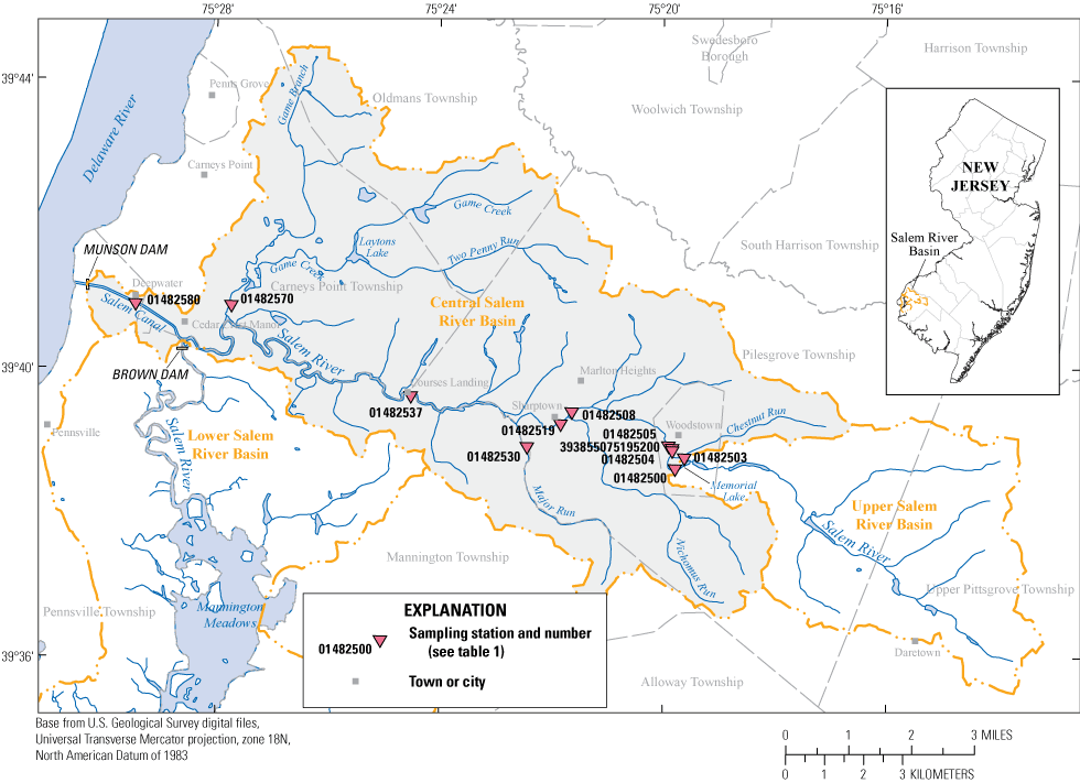
Map showing location of study area, central Salem River Basin, New Jersey.
Eutrophication is a complex environmental process whereby water bodies, particularly slow-moving streams or lakes, become enriched with dissolved nutrients that stimulate excessive growth of aquatic photosynthetic organisms, which form the base of the food web (Munn and others, 2018). The remaining discussion in this paragraph was derived mainly from Ji (2008) and Chapra (1997). These primary producers can use light, carbon dioxide, and nutrients to synthesize new organic material. These organisms can be free floating (phytoplankton), attached (periphyton), or floating/attached larger plants (macrophytes). Such growth causes wide diurnal variations in dissolved-oxygen (DO) concentrations, with high concentrations during the day (when photosynthesis occurs) and low concentrations at night (when respiration occurs). Excessive growth commonly results in a “die-off” of plants and organisms that leads to increased biochemical oxygen demand (BOD) and sediment oxygen demand (SOD), which can compromise the health of fish, benthic macroinvertebrates, and other aquatic species. Eutrophication can result in decreased biodiversity and loss of desirable fish species, and otherwise impair the biotic integrity of aquatic ecosystems supported by a river (Wurtsbaugh and others, 2019). Phytoplankton chlorophyll-a (CHL-a), a component of photosynthetic organisms, is commonly used as an indicator of this growth by measuring the algal mass. Nutrients that promote excessive growth are derived from a variety of sources, including fertilizers applied to lawns and agricultural fields, and sewage discharged from treatment facilities. Ammonia is of particular concern because it reacts chemically with oxygen, further reducing the concentration of DO and can be toxic to fish.
A load-duration curve is a simple graphical tool that illustrates the relation between nutrient load and the probability of exceeding the load in a water body. Load-duration curves are useful in TMDL analysis because they establish loading capacities for a range of flow conditions (U.S. Environmental Protection Agency, 2007c). A phosphorus load-duration curve for the Salem River at Woodstown, N.J. (station 01482500) is shown in figure 2. Phosphorus is used as an example because it is a primary nutrient of interest in the Salem River and a possible candidate for a TMDL. Water-quality data for 1998 to early 2008 (46 samples) and daily flow data for the same period were derived from the National Water Information System (NWIS) database (U.S. Geological Survey, 2022). The curve representing the maximum allowable load was constructed by multiplying the streamflow for the station by the total-phosphorus surface-water-quality standard for nontidal streams of 0.1 milligram per liter (mg/L) (State of New Jersey, 2020, p. 28) and a conversion factor to produce units of load in pounds per day. Salem River is classified FW2-NT—freshwater not designated FW1, nontrout stream (State of New Jersey, 2020, p. 77). Computed loads based on sample-analysis results that plot above the curve indicate noncompliance under certain flow conditions, whereas computed loads that plot below the curve indicate compliance with the surface-water-quality standard. Because load-duration-curve analysis accounts for streamflow variability, it can be a useful indicator of hydrologic conditions that prevail when a water body is out of compliance.
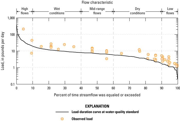
Graph showing load-duration curve for total phosphorus at station 01482500, Salem River at Woodstown, New Jersey.
On the basis of the load-duration curve in figure 2, available data indicate that TP exceeds the surface-water-quality standard of 0.1 mg/L, and therefore TP is likely a driver of eutrophication in the central Salem River. All but two computed loads fall above the line representing the surface-water-quality standard for phosphorus. Frequency of noncompliance appears to be unrelated to streamflow magnitude, as phosphorus loads exceed the standard across the full range of flows measured at the site, indicating that phosphorus may be derived from several sources.
Duration curve analysis uses intervals, which can be a general indicator of hydrologic conditions (for example, wet versus dry and to what degree). Intervals can be grouped into several categories or zones. These zones provide additional insight about conditions associated with the impairment (U.S. Environmental Protection Agency, 2007c). Exceedances for mid-range, wet, and high-flow conditions are likely a result of basin runoff processes that transport phosphorus from urban and cropland and deliver it to the main-stem river during storm events, and resuspension of benthic-sediment phosphorus through scour. Exceedances for dry or low-flow conditions typically represent steady sources of phosphorus that might include groundwater contributions and wastewater effluent. Additionally, benthic release into the water column may contribute to elevated phosphorus concentrations during dry conditions.
Although the load-duration approach is useful for assessing the frequency and severity of noncompliance, determining which flow conditions most often accompany periods of noncompliance, and inferring potential constituent sources, it cannot be used to test watershed-management strategies or determine the effects of changes in land use, climate, or water use on nutrient levels in the Salem River. A water-quality model is needed to account for chemical, biological, and physical processes that affect the fate and transport of nutrients in the river. A properly constructed and calibrated model provides a rigorous framework with which to test a variety of possible management scenarios. The model also can account for short-term changes in water use and long-term changes in the hydrologic regime caused by alterations in land use and climatic conditions. Because the surface-water-quality standard for TP has been exceeded at several locations in the central Salem River, NJDEP determined that a surface-water-quality model is warranted to investigate this impairment and help develop a nutrient TMDL for the river. Therefore, the U.S. Geological Survey (USGS), in cooperation with the NJDEP, configured such a model and calibrated it to field data collected from April 2007 to October 2008. This report documents the development and calibration of the model and the simulation of two management scenarios.
Purpose and Scope
This report documents the results of a study whose objectives were to (1) assess available data collected as part of an associated monitoring study of the central Salem River, (2) supplement those data through additional monitoring, (3) develop a surface-water-quality model of the central Salem River to serve as a tool for evaluating nutrient-loading processes and identifying nutrient sources, and (4) use the model to test alternative management scenarios for establishing a nutrient TMDL for the river. The EPA Water Quality Analysis Simulation Program (WASP) model (Wool and others, 2003) was used for the simulation. The surface-water-quality model consists of two components—a flow model and a water-quality model. This report documents data collection, estimation of model inputs where data were lacking, development and calibration of the flow model, development and calibration of the water-quality model, assessment of model limitations and applicability, and development and testing of two management scenarios. Model validation is possible by using a separate dataset or a subset of the main dataset when sufficient data are available; however, this condition was not met for this study.
Description of Study Area
Salem County is in southwestern New Jersey, in the Coastal Plain Physiographic Province (fig. 1). According to the 2020 United States Census, it ranks as the least populated county in New Jersey, with only 0.7 percent of the State’s population (64,837 people) residing within its boundaries (New Jersey Department of Labor and Workforce Development, 2021). The land area of 331.9 square miles (mi2) occupies 4.5 percent of the total area of the State (New Jersey Department of Labor and Workforce Development, 2021). Despite its small size and population, Salem County ranked 3rd out of 21 New Jersey counties in market value of agricultural products sold in 2012 (U.S. Department of Agriculture, 2012).
Salem River is an approximately 30-mile- (mi) long tributary of the Delaware River located entirely within Salem County. The headwaters of the Salem River are near Daretown, and the river flows downstream through a series of small impoundments before reaching Memorial Lake at Woodstown (fig. 1). For the purposes of this study, the area upstream from the outlet of Memorial Lake is considered to be the upper Salem River Basin. The study area, the central Salem River Basin (44.2 mi2), extends from the outlet of Memorial Lake westward to Brown and Munson Dams near Deepwater. The dams separate the nontidal and tidal reaches of the Salem River. Brown Dam redirects flow westward toward Salem Canal and away from the historical south-flowing channel to the city of Salem (Lower Salem River Basin). Salem Canal is an approximately 2-mi-long structure built to provide feedwater storage to DuPont Chambers Works. At the downstream end of the Salem Canal is Munson Dam, which releases water through gates to the Delaware River.
Main-stem reaches of the Salem River in the study area are characterized by two distinct hydrologic regimes. Reaches upstream from the confluence with Major Run tributary are predominantly riverine and are subject to different flow dynamics than low-energy reaches below the confluence with Major Run, which are primarily lacustrine as a result of backwater from Munson and Brown Dams. Backwater also extends upstream into Game Creek. Although riverine reaches may exhibit higher energy than lacustrine reaches, their flow velocities are generally low as a result of the overall shallow slope of the channel. Topographic relief in the study area is low, with land-surface altitudes ranging from greater than 46 meters (m) or 151 feet (ft) above NGVD 29 near Daretown to near sea level at the confluence of the Salem and Delaware Rivers. Land use in the central Salem River Basin is predominantly agricultural (approximately 53 percent of the area) (fig. 3). Other land uses include water/wetland (23 percent), urban (13 percent), forest (10 percent), and barren (1 percent).
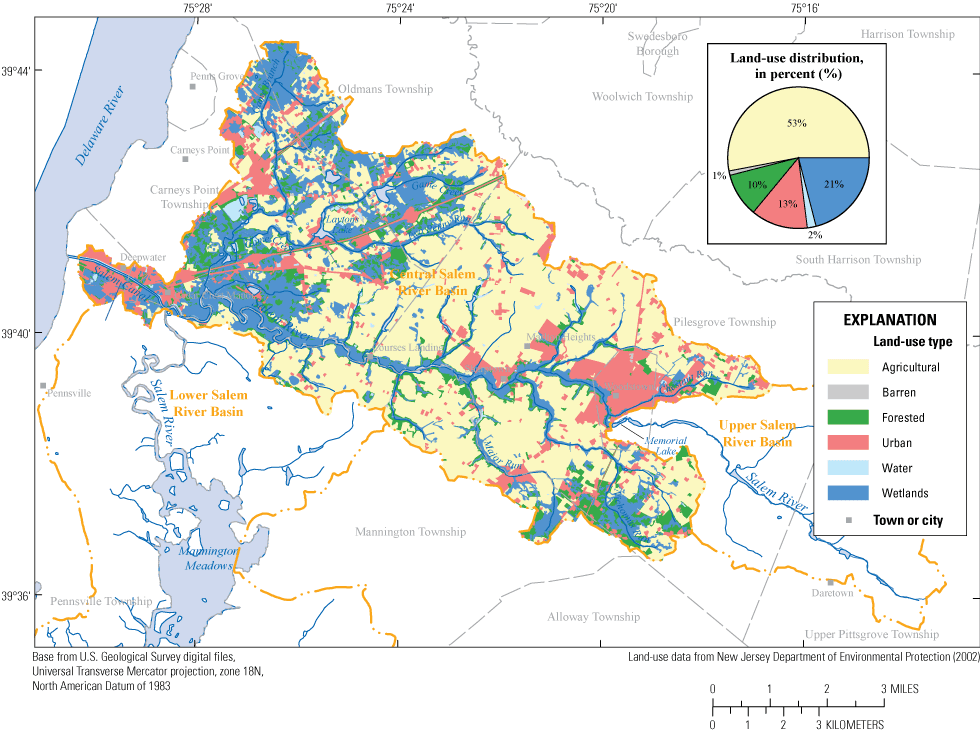
Map showing generalized land-use distribution in the central Salem River Basin, New Jersey, 2007–08.
The growing season in Salem County can be defined as the time between the historical dates of first and last frost (April 20 to October 20) (U.S. Department of Agriculture, 2008, p. 185) or as the period during which conditions are most favorable to algal growth (June 1 to September 1) (Barbara Hirst, N.J. Department of Environmental Protection, written commun., 2010). The former period was used in this study and is referred to as the growing season.
Previous Studies
Najarian Associates (1990) developed a surface-water-quality model of the Salem River to predict the response in water quality to an anticipated increase in wastewater discharge from the Woodstown Wastewater Treatment Plant (WWTP). Rutgers Cooperative Extension (2012) developed a watershed restoration and protection plan for the upper Salem River Basin. Baker and Esralew (2010) computed concentrations and loads of water-quality constituents from storm- and base flows in six streams, including one in upper Salem County, in several land-use areas in the lower Delaware River Basin in 2002–07. Hunchak-Kariouk and others (1999) determined relations between water quality and streamflow for constituents at 14 surface-water-quality stations and associated trends through time during high and low flows in the lower Delaware River Basin, including the Salem River, for water years 1976–93 (a water year is defined as the 12-month period October 1, for any given year through September 30, of the following year, and is designated by the calendar year in which it ends). New Jersey Department of Environmental Protection (2003a) established TMDLs for TP that address eutrophication in lakes in the lower Delaware Water Region (New Jersey Watershed Management Areas 17–20), including Memorial Lake at Woodstown.
Data Collection
Limited historical water-quality data were available for the central Salem River Basin; therefore, a primary monitoring study was conducted by the USGS in 2007–08 to support understanding of nutrient loading processes as well as to provide data for development of a surface-water-quality model. All data described in this report can be accessed in the NWIS database (U.S. Geological Survey, 2022) or are available in a USGS data release (DePaul and Spitz, 2023). As part of this data-collection effort, in situ SOD and sediment phosphorus and carbon concentrations were measured during July–August 2008 (Heckathorn and Gibs, 2010). The primary monitoring was supplemented by selected data collected during late summer 2008. Data collected during 2007–08 are summarized in table 1 and discussed below. Long-term monitoring for DO and other environmental parameters has been conducted at station 01482500, Salem River at Woodstown, since 2001 as part of the New Jersey Ambient Surface Water Quality Monitoring Network. Data are available in the NWIS database (U.S. Geological Survey, 2022).
Table 1.
Sampling stations and types of data collected in the central Salem River Basin, New Jersey, 2007–08.[Bold indicates tributary station; SOD, sediment oxygen demand; CBOD, carbonaceous biochemical oxygen demand; N.J., New Jersey; X, data collected; --, not applicable; WWTP, wastewater-treatment plant]
| Station number (Locations shown in fig. 1) | Station name | Primary sampling, July 2007 to August 2008 | Supplemental sampling, August–September 2008 | Continuous monitoring, August–September 2008 | ||||||
|---|---|---|---|---|---|---|---|---|---|---|
| Field parameters1 | Laboratory parameters1 | SOD2 | Bed-sediment phosphorus1 | Vertical profile3 | Nutrients, CBOD1, 3 | Light extinction3 | ||||
| 401482500 | Salem River at Woodstown, N.J. | X | X | -- | X | -- | Mid-depth | X | -- | |
| 01482503 | Chestnut Run at Woodstown, N.J. | X | X | -- | X | -- | -- | -- | -- | |
| 01482504 | Salem River above WWTP at Woodstown, N.J. | -- | -- | -- | -- | -- | -- | -- | Long term | |
| 393855075195200 | Woodstown WWTP effluent | X | X | -- | -- | -- | -- | -- | -- | |
| 01482505 | Salem River at Woodstown/Route 40, N.J. | X | X | -- | X | -- | -- | X | -- | |
| 01482508 | Salem River at Sharptown/Route 40, N.J. | X | X | -- | X | -- | -- | X | -- | |
| 01482519 | Salem River at Sharptown/Main Street, N.J. | X | X | X | X | -- | -- | X | Short term | |
| 01482530 | Major Run at Sharptown, N.J. | X | X | X | X | -- | -- | -- | Short term | |
| 01482537 | Salem River at Courses Landing, N.J. | X | X | X | X | X | Shallow and deep | X | Long term | |
| 01482570 | Game Creek near Deepwater, N.J. | X | X | -- | X | -- | -- | X | -- | |
| 01482580 | Salem Canal at Deepwater, N.J. | X | X | -- | -- | X | Shallow and deep | X | -- | |
USGS National Water Information System database (U.S. Geological Survey, 2022). Field parameters include water temperature, dissolved oxygen, dissolved-oxygen saturation, specific conductance, pH, and turbidity. Laboratory parameters include total phosphorus, dissolved inorganic phosphorus, total Kjeldahl nitrogen, ammonia, nitrate, total dissolved solids, total suspended solids, acid neutralizing capacity, chlorophyll-a (phytoplankton), CBOD (5-day, 20-day), and total organic carbon. Composite sampling was done at Woodstown WWTP (393855075195200). Long-term continuous data vary in duration; short-term continuous data are less than 3 days. Continuous parameters were the same as field parameters, except for turbidity.
DePaul and Spitz (2023). Vertical-profile parameters were the same as field parameters, except for turbidity. Light-extinction data were collected by using Secchi disk at Courses Landing (01482537) and Salem Canal (01482580), including in September 2009. Intermittent-sampling data were available from Woodstown WWTP (393855075195200) and DuPont Chambers Works diversion (near 01482580).
Additionally, quarterly sampling data were available from N.J. Ambient Surface-Water-Quality Monitoring Network (U.S. Geological Survey, 2022).
Monitoring Data
The 2007–08 monitoring provided some flow data required for modeling. Streamflow measurements were made at the sites of water-quality-sample collection. Flow measurements were not possible at some locations (for example, Game Creek, Salem Canal) as a result of low flow velocities. Continuous stage data were collected during August 2008–October 2008 to estimate continuous discharge at the farthest downstream sampling location (Salem Canal, 01482580); however, the relation between stage and discharge could not be determined as a result of various difficulties encountered, such as flow velocities too low to measure, insufficient information on the operation of Munson Dam gates, and inability to obtain accurate data on the Salem Canal diversion. Land-surface altitudes surveyed in October 2008 were used to calculate the slope of the river channel throughout the study area.
During the 2007–08 monitoring study, water-quality samples were collected during base-flow and high-flow conditions (table 1). Samples were collected at 10 stations along the main-stem river (fig. 1). At each station, samples were collected at least nine times to characterize water quality during the growing season. Measurements of basic field parameters, including water temperature, DO, pH, and specific conductance, were made during each site visit. Nutrient species, chlorophyll-a (CHL-a), and carbonaceous biochemical oxygen demand (CBOD) were analyzed for each sample. Biochemical oxygen demand (BOD), which is composed of CBOD and nitrogenous biochemical oxygen demand (NBOD), is a measure of the potential of receiving waters to deplete the oxygen level and is commonly used to determine the extent to which a waste stream (for example, from a WWTP) could affect a receiving water by depriving aquatic organisms of oxygen. Because samples were not collected for analysis of NBOD, this parameter could not be directly simulated. Secchi depth was measured at seven stations to evaluate light extinction in the water column. Most of the Secchi depth measurements were made at Courses Landing and Salem Canal; six measurements were made at each of these two stations.
In addition to discrete sampling, short-term (3-day) continuous monitoring was conducted at three sites (Sharptown, Major Run, Courses Landing) to characterize diurnal variations in DO concentration and water temperature. Also, effluent from the Woodstown WWTP was characterized by analyzing eight 24-hour composite samples for nutrients. SOD, the rate of oxygen consumption exerted by bottom sediment on the overlying water, was measured at three sites in lacustrine reaches on a multiday basis to characterize exchange between the sediments and the water column as a result of sediment diagenesis (Heckathorn and Gibs, 2010). Riverbed sediment was sampled twice during summer 2008 and analyzed for TP and total carbon (TC) at seven stations. Additionally, TP was measured once at an eighth station.
Supplemental monitoring was conducted during August and September 2008 to support water-quality modeling (table 1). Discrete sampling, involving eight biweekly synoptic surveys, was conducted at Woodstown, Courses Landing, and Salem Canal, which were critical sites for NJDEP for characterizing variations in DO, nutrients, and CBOD. Additional data collection at Courses Landing and Salem Canal included surface and depth samples to characterize the water column vertically. Six concurrent 5-day and 20-day CBOD samples were collected to compute the CBOD decay rate. Twenty-day CBOD was used as proxy for (long-term) ultimate CBOD (CBODu) in the WASP model. Continuous monitoring was conducted at Woodstown (deep) and Courses Landing (shallow and deep) to characterize diurnal variations in DO and differences with depth.
Reported Data
Additional data needed for the model were obtained from public and private sources. Time-of-travel measurements for the Salem River were available from USGS dye tracer tests conducted during the fall of 1974. Reported flow data were compiled for the Woodstown WWTP and Salem Canal diversion (DuPont Chambers Works). Woodstown WWTP provided effluent NH4 and TP concentrations for samples collected approximately weekly. DuPont Chambers Works provided intake water quality from Salem Canal, from which daily water temperature was obtained. A gate operation schedule for Munson Dam also was obtained. Brown Dam has flashboards, and not gates, thus no data were available. All of the above data are included in the data release associated with this report (DePaul and Spitz, 2023), with the exception of gate operation data, which are not used in the model. Limited model-input and calibration data were obtained from the previous study by Najarian Associates (1990).
Water-Quality Conditions
Ranges in concentrations of selected water-quality constituents in the main-stem Salem River and Chestnut Run, Major Run, and Game Creek tributaries are listed in table 2. Boxplots in figure 4 show concentrations of DO, nutrients, and CHL-a. The following sections examine ambient water quality in the Salem River Basin with respect to selected constituents based on these data.
Table 2.
Summary concentration statistics for selected constituents in the central Salem River, New Jersey, 2007–08.[Source of data is National Water Information System database (U.S. Geological Survey, 2022); concentrations are in milligrams per liter, except for chlorophyll-a, which is in micrograms per liter; statistics are for growing season only, April 20 to October 20. <, less than]
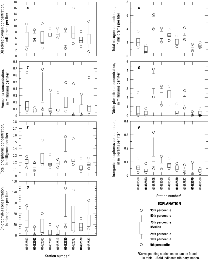
Boxplots showing concentrations of selected water-quality parameters at sampling stations on the Salem River and tributaries, New Jersey, 2007–08.
Water Temperature
Water temperatures throughout the main-stem river during the growing season ranged from 13.1 to 29.4 degrees Celsius (°C). Water temperatures were typically highest from July through September, when air temperatures were highest and stream discharge was approaching the seasonal minimum. Seasonal median water temperatures were highest at Courses Landing and Salem Canal (23.6 and 25.4 °C, respectively), likely as a result of stagnant flow conditions and lack of shade. Seasonal median water temperatures were lowest at the two sites near Sharptown (20.5 and 19.9 °C), which can be explained by a combination of factors, including dense tree canopy that shades the water surface, rapidly flowing water that heats less quickly in riverine reaches than in lacustrine reaches, and possible contributions from inflow of colder groundwater. Differences in water temperature with depth at Courses Landing were as large as 4 °C during the growing season, which may be sufficient to impede mixing and indicates some degree of stratification. Seasonal median water temperatures in the tributaries ranged from 19.8 to 23.8 °C, with the highest water temperatures measured at Game Creek, a tributary that periodically experiences near-stagnant flow conditions.
Dissolved Oxygen
Discrete DO measurements in the main-stem Salem River (fig. 4A) ranged from less than 2 to nearly 16 mg/L. The range in DO variation was greatest during the growing season and was generally less than 2 mg/L in riverine segments but as much as five times that in lacustrine segments, which exceeds the NJDEP guidance level of 3 mg/L over the course of a day. Seasonal median DO concentrations were within a normal range of 6 to 8 mg/L at many sites, although values at Woodstown, Salem Canal, and Game Creek approached the surface-water-quality standard of not less than 4.0 mg/L at any time (State of New Jersey, 2020, p. 26) about 25 percent of the time. These lower quartiles are likely associated with greater eutrophication and predominance of consumptive DO processes (algal respiration, CBOD, SOD) in lacustrine main-stem and slow-flowing tributary reaches than in riverine reaches. DO concentrations were highest at Woodstown (13.6 mg/L), Courses Landing (16 mg/L), and Salem Canal (12.0 mg/L), although some of the lowest values (less than 4 mg/L) were also measured at these sites. Large variations in DO concentration are typical of eutrophic conditions, with high concentrations observed during the day when photosynthetic production of DO occurs and low concentrations observed at night during cellular respiration, or during periods of die-off and decomposition (Ji, 2008). High seasonal median and a narrow interquartile range in DO concentration were observed at the two water-quality stations near Sharptown (01482508 and 01482519), where conditions such as tree shade and swiftly moving water are not conducive to eutrophication. Salem River at Woodstown and Game Creek were the sites where DO concentrations were most frequently less than 4 mg/L. In other main-stem reaches and tributaries, DO concentrations were sometimes less than 4 mg/L, although the value typically did not violate the surface-water-quality standard of 24-hour average not less than 5.0 mg/L (State of New Jersey, 2020, p. 26). Seasonal median DO concentrations were lowest from July through September in both the main-stem river and tributaries. Concentrations at tributary stations ranged from 2.5 to 9.0 mg/L, with a seasonal median of 4.6 mg/L.
Continuous and intensive DO measurements collected at selected stations in the central Salem River during late summer of 2008 are shown in figure 5. DO concentrations near the bottom of the water column (75-percent depth) at Woodstown were frequently at or less than 4 mg/L, even during daylight hours, and the diurnal variation was typically less than 2 mg/L (fig. 5A). Undersaturation of DO at this location throughout much of this period suggests that consumptive DO processes exceed productive DO processes. Median concentration and percent saturation during the measurement period were 3.8 mg/L and 44 percent, respectively. DO concentrations near the surface (30-percent depth) at Courses Landing ranged from about 4 to 16 mg/L and varied diurnally as much as 8 mg/L during August 2008 (fig. 5B). DO concentrations also were measured near the bottom of the water column (60-percent depth). Supersaturation of DO (130–200 percent relative to air) typically occurred during afternoons, when productivity was high. DO concentrations decreased sharply at all sites in early September 2008. This decline was preceded by a storm event, which likely introduced suboxic waters from adjacent wetlands into the river. Nutrients flushed from the river during the storm and colder-than-normal air temperatures beginning in early September likely inhibited algal growth, resulting in lower DO concentrations and smaller diurnal variations.
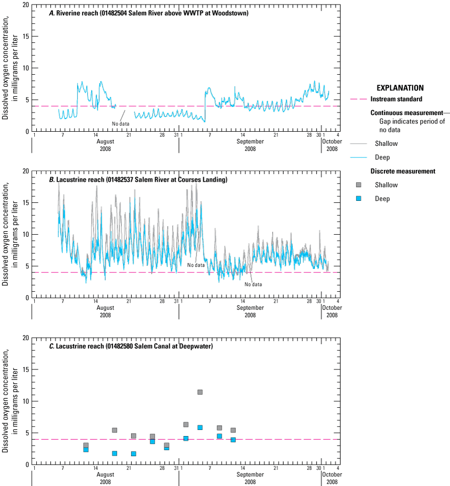
Graphs showing spatial and temporal variations in concentration of dissolved oxygen in riverine and lacustrine reaches of the central Salem River, New Jersey, August–October 2008.
Vertical profiles of DO and water temperature were measured in lacustrine reaches (fig. 6) (DePaul and Spitz, 2023). Water temperature in these reaches often decreased with depth; therefore, the solubility of gas should increase. However, temperature differences of only a few degrees between surface and subsurface waters are sufficient to impede mixing and isolate the lower portion of the water column (Wetzel, 2001). As stratification is established, DO is depleted by biochemical oxygen demands in the lower water column exerted by sediment (SOD), CBOD is generated as a result of phytoplankton death or other oxidizable matter, and light attenuation suppressing photosynthetic activity. By mid- and late summer, DO concentrations in the lower water column are substantially lower than those in the upper water column, and anoxic conditions can occur near the sediment/water interface. DO concentrations in lacustrine reaches of the central Salem River were high in the upper water column and reduced in the lower water column. DO concentrations differed vertically by over 5 mg/L on average, and up to 10 mg/L at Courses Landing and Salem Canal during periods of peak photosynthetic activity (fig. 6). Diurnal variations were smaller and median concentrations were lower at depth than at the surface at Courses Landing, perhaps as a result of this stratification.
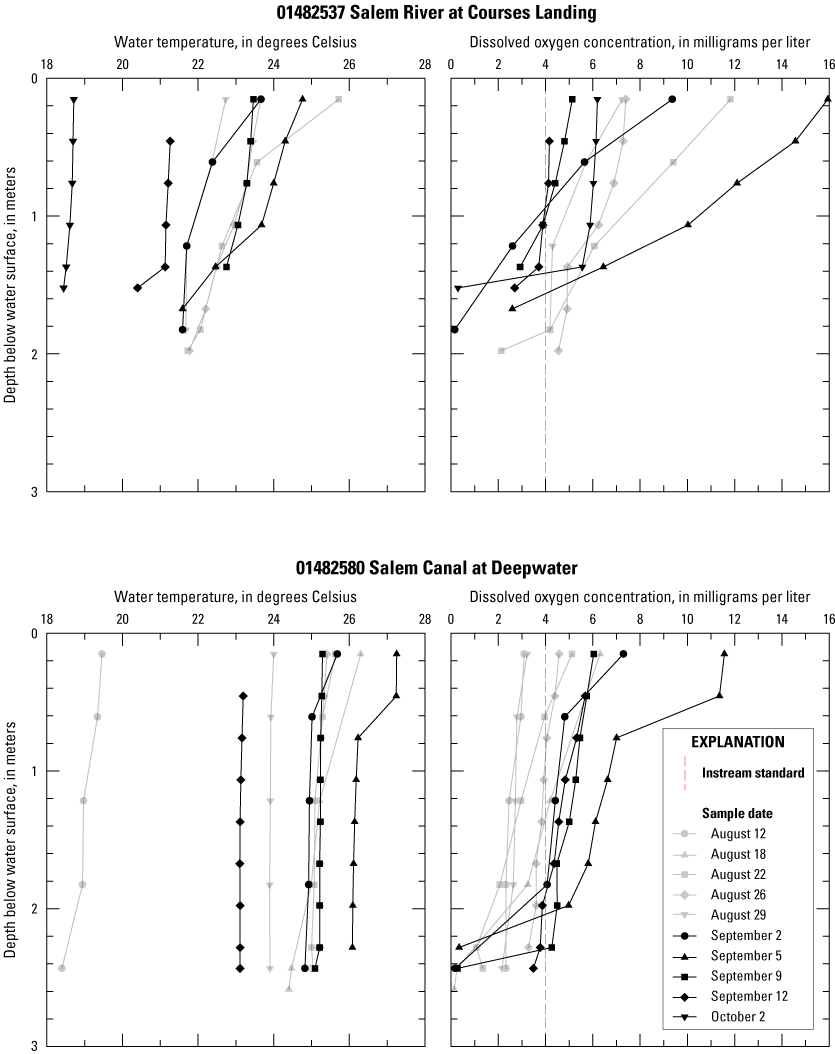
Graphs showing vertical profiles of water temperature and concentration of dissolved oxygen in lacustrine reaches of the central Salem River, New Jersey, August–October 2008.
Nitrogen
Water samples collected from the central Salem River exhibited moderate to high TN concentrations relative to natural background concentrations. Upper-quartile TN concentrations were typically less than 0.65 mg/L as determined by statistical examination of analyses of samples from predominantly undeveloped basins in the New Jersey Coastal Plain. Empirical models for determining background concentrations of nutrients in rivers and streams in basins in the U.S. Eastern Coastal Plain Ecoregion (Smith and others, 2003) estimated similar upper-quartile TN concentrations of 0.63 mg/L.
TN concentrations in water samples from the main-stem river ranged from 1.23 to 6.13 mg/L (table 2, fig. 4B). Seasonal median TN concentrations were 2.7 mg/L at stations on the main-stem river and highest just downstream from the Woodstown WWTP outfall and lowest in Salem Canal. Seasonal median concentrations were greater than 2 mg/L in the main-stem river between the Woodstown WWTP and Courses Landing but were less than 2 mg/L at Woodstown, Salem Canal, and the three sampled tributaries. Concentrations at tributary stations ranged from 0.43 to 2.96 mg/L, with a seasonal median of 1.45 mg/L. Concentrations at most main-stem river stations and the three tributaries were highest during the nongrowing season when biological uptake is lowest and lowest during late summer when biological uptake is highest.
NH4 and NO3 are the nitrogen forms most available for uptake by algae and other aquatic plants. NH4 concentrations ranged from less than 0.04 to 0.69 mg/L in the main-stem river, with a seasonal median of 0.11 mg/L (table 2, fig. 4C). Concentrations were highest just downstream from the Woodstown WWTP outfall. Concentrations were slightly higher at lacustrine stations such as Courses Landing and Salem Canal than at riverine stations such as Sharptown, possibly as a result of biochemical transformations in lacustrine reaches and (or) fertilizer application in adjacent watersheds. Concentrations generally peaked during late summer, although marked seasonal variations were absent. Concentrations at tributary stations ranged from less than 0.04 to 0.49 mg/L, with a seasonal median of 0.10 mg/L, and generally were highest in Major Run (median approximately 0.25 mg/L).
NO3 concentrations ranged from less than 0.04 to 5.17 mg/L in the main-stem river, with a seasonal median of 1.38 mg/L (table 2, fig. 4D). The highest NO3 concentrations ranged from about 1 to 5 mg/L at stations between the Woodstown WWTP and Courses Landing, and the lowest concentrations ranged from about 0.02 to 1 mg/L at Woodstown and Salem Canal. NO3 concentrations in samples collected at these two stations were low in relation to those of NH4 and DON during the summers of 2007 and 2008, which may be an indicator of biological uptake, denitrification, or physical removal. NO3 concentrations were highest during fall and winter and lowest during August and September. The station just downstream from the Woodstown WWTP outfall exhibited a smaller annual variation as a result of the relatively constant NO3 concentration in effluent. NO3 concentrations at tributary stations ranged from less than 0.04 to 1.30 mg/L, with a seasonal median of 0.14 mg/L, and were highest in Major Run and lowest in Game Creek. Spatial and temporal patterns of NO3 were similar to those of TN because NO3 accounted for a large portion of TN. Concentrations did not exceed the surface-water-quality standard of 10 mg/L for NO3 (State of New Jersey, 2020, p. 38) at any of the sampling sites.
Phosphorus
Water samples collected from the central Salem River exhibited elevated TP concentrations relative to natural background concentrations. Upper-quartile TP concentrations were 0.04 and 0.02 mg/L as determined by statistical examination and empirical models described in the last section, respectively.
TP concentrations ranged from 0.11 to 0.55 mg/L in the main-stem river, with a seasonal median of 0.2 mg/L (table 2, fig. 4E). Concentrations were highest just downstream from the Woodstown WWTP outfall and at Courses Landing. Concentrations were highest during the growing season, particularly in July and August. Concentrations at tributary stations ranged from 0.06 to 0.58 mg/L, with a seasonal median of 0.17 mg/L, and were highest in Major Run and lowest in the other two sampled tributaries, a result that applied to all sampled constituents. Almost all samples exceeded the surface-water-quality standard of 0.1 mg/L at all main-stem river stations and Major Run.
DIP is the phosphorus form most available for uptake by algae and other aquatic plants. DIP concentrations ranged from 0.01 to 0.32 mg/L in the main-stem river, with a seasonal median of 0.05 mg/L (table 2, fig. 4F). Concentrations were highest just downstream from the Woodstown WWTP outfall and lowest in Chestnut Run, Game Creek, and Salem Canal. Concentrations at tributary stations ranged from 0.01 to 0.1 mg/L, with a seasonal median of 0.04 mg/L. TP is nearly 30 percent DIP in main-stem riverine reaches; the percentage is slightly less in main-stem lacustrine reaches.
Unlike nitrogen, which is highly soluble, phosphorus is poorly soluble and is strongly sorbed to suspended solids. As a result, a large volume of phosphorus can enter the main-stem river attached to particles of inorganic sediment and organic matter. Concentrations of particulate-bound TP as high as 90 mg/g sediment were reported in Salem Canal, whereas concentrations of dissolved TP were typically less than 0.02 mg/L, as determined from samples collected on April 7, 2008. In this case, more than 4.5 times as much TP (per liter) was associated with suspended sediment than was dissolved in water (at a typical low-flow suspended-sediment concentration of 1 mg/L). Even larger differences are possible during stormflow. Slow flow velocities can allow solids and organic material to settle to the riverbed; as a result, a store of phosphorus can build up in riverbed sediment over time, as indicated by the greater concentrations measured in lacustrine reaches than in riverine reaches (fig. 7). A similar result is observed for riverbed TOC (Heckathorn and Gibs, 2010, table 4).
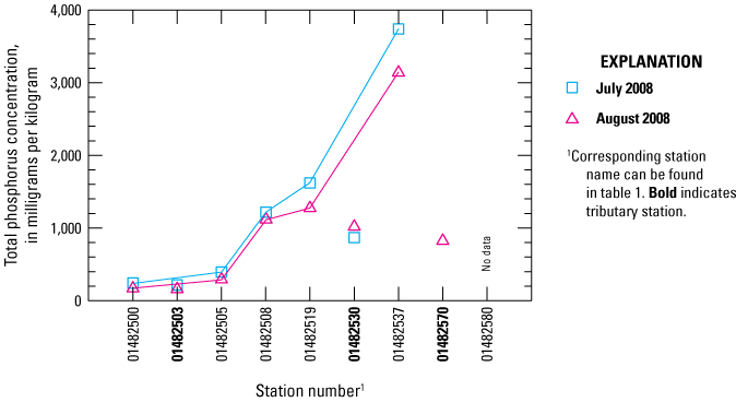
Graph showing spatial variation in concentration of total phosphorus in riverbed sediment in the central Salem River and tributaries, New Jersey, July–August 2008.
Phytoplankton Chlorophyll-a
An excess of nutrients in a water body can promote the growth of floating (phytoplankton) and attached (periphyton) algae, and floating and attached plants (macrophytes) (Ji, 2008). Algae produce oxygen during the day through photosynthesis and consume oxygen at night through respiration, causing a diurnal signal in DO concentration. Algal growth is enhanced by environmental factors such as excessive availability of nutrient species, increased light, and increased water temperature, and physical factors such as reduced water velocity (increased residence time). Algae ultimately die and are recycled for uptake by living algae as part of the overall nutrient cycling process. A pigment found in many photosynthetic organisms, CHL-a, is used as a gross measure of the living phytoplankton population and a measure of impairment of a water body. Phytoplankton CHL-a was used as a measure of biomass in this study, although no taxonomic data were collected.
CHL-a concentrations ranged from less than 1 to 126 µg/L in the main-stem river, with a seasonal median of 19 μg/L (table 2, fig. 4G). Concentrations in the main-stem river at Woodstown, Courses Landing, and Salem Canal were much higher than at other stations, with medians exceeding 30 µg/L and maximums exceeding 80 µg/L. Concentrations near Sharptown and in Chestnut Run were much lower, with medians less than 5 µg/L and maximums less than 30 µg/L. Concentrations at the station downstream from Woodstown WWTP were intermediate, with a median near 15 µg/L and a maximum greater than 60 µg/L, likely from algal blooms in Memorial Lake that wash over the dam spillway into upper riverine reaches. Concentrations in riverine reaches downstream from this station were lower as a result of algal die off. Heavy tree canopy, cooler water temperatures, and rapid transport inhibit opportunities for algal growth. Salem River widens near its confluence with Major Run and receives more light; downstream damming retards flow and increases retention time, which creates conditions conducive to growth. Game Creek is characterized by less agricultural influence, increased light transparency, slow flow velocity, and more natural substrate, which may help explain the abundant macrophyte growth along the upper reaches of the creek (Dar and others, 2014). CHL-a concentrations ranged from 2 to 131 μg/L at tributary stations, with a seasonal median of 23 μg/L; they were highest in Major Run.
CHL-a concentrations in the main-stem river typically were highest during July and August of the study period, although they exceeded 70 μg/L in Salem Canal as late as mid-October 2007. No surface-water-quality standard has been established for phytoplankton CHL-a, but an instream threshold of 24 μg/L has been used as an indicator of impairment (Marzooq Al-Ebus, N.J. Department of Environmental Protection, oral commun., 2010). This concentration may not ultimately be adopted as the TMDL threshold; an appropriate threshold, possibly with a temporal component, will be set through additional collaboration and research with NJDEP. CHL-a concentrations were at or above this threshold at most sampling locations, indicating substantial algal productivity.
Simulation of Flow and Eutrophication
WASP version 7.3 (Wool and others, 2003) was selected for use in the simulation of flow and water quality in the central Salem River. WASP is a dynamic compartment model for aquatic systems that allows for exchange between the water column and the underlying benthos. WASP provides a generalized framework for predicting the fate and transport of constituents (state variables) in up to three dimensions for linear and nonlinear water-quality problems. WASP solves a mass-balance equation describing concentrations of dissolved constituents in a water body that accounts for advective and dispersive transport; material entering and leaving through direct and diffuse loading; and physical, chemical, and biological transformations in the water body. Additional details about WASP are available in the model documentation (Wool and others, 2003; Wool and Ambrose, 2006; Wool and others, 2008). Definitions of terminology used in the WASP model also can be found in the documentation and in other references on water quality models (for example, U.S. Environmental Protection Agency, 1997).
WASP is a receiving water model, in contrast to a watershed model, in that flow and water quality processes are not simulated in upland areas, but rather are accounted for indirectly as inputs to a main stem river model. River reaches are represented in WASP as a series of discrete computational elements (segments, control volumes) with chemical concentrations assumed to be uniform within each element. Each simulated constituent is advected and dispersed as it moves from one segment to the next and acted on through kinetic reactions. Sorbed fractions may settle through water-column segments. Dissolved constituents are exchanged with benthic segments representing the riverbed through a diffusive mixing process. Simulation of eutrophication processes in WASP can be configured at various levels of complexity to represent environmental processes involving transport and interaction among DO, oxygen demands, phytoplankton, and nutrients. The WASP advanced eutrophication module was used for the central Salem River model.
Model Design
The model domain encompasses the central Salem River Basin (44.2 mi2) from the Woodstown gaging station (01482500) to Munson Dam on Salem Canal and is similar to the model domain used by Najarian Associates (1990). The upper Salem River Basin (14.4 mi2) was not included in the model because it was outside the 2007–08 monitoring study area; however, constituent loads representative of the Upper Salem River Basin were computed for the upstream model boundary. Tidal portions of the Salem River below Munson and Brown Dams were not included in the model. Game Creek, the largest tributary in the study area, was simulated in the model, but only the eastern fork as far as Laytons Lake; the western fork (Game Branch) was not included so that the tributary could be modeled as a single reach (fig. 1). The eastern fork was represented by two reaches—a short reach at the outlet of Laytons Lake and a long reach downstream to the confluence with the Salem River—to isolate the boundary condition from the remainder of the reach. Including Game Creek in the model partially accounts for the effects of dilution from this large tributary to the Salem River.
The study area was discretized into 21 model segments (fig. 8)—20 water-column segments and 1 surface benthic segment—on the basis of several factors, including location of data-collection sites (fig. 1), delineated subbasin boundaries, and flow considerations (table 3). Subbasin boundaries were delineated in ArcGIS software by using a 10-meter (32.8-foot) digital elevation model, a stream-reach coverage, and a pour (outlet) point coverage. Impoundment of the lower Salem River by Munson and Brown Dams results in low flow velocities in downstream river reaches; therefore, approximately two-thirds of the study area is represented by a narrow flow-through lake rather than a river channel. Accordingly, riverine reaches are represented by shallow, single-layer segments numbered 1 through 8. Most lacustrine reaches are represented by deep, two-layer segments to account for vertical movement in the water column. Upper water-column segments are numbered 9, 10, and 12 through 14, and lower water-column segments are numbered 16 through 20. Upper and lower water-column segments were used in lacustrine reaches also to account for vertical differences in water quality. Segment 11 is a single-layer lacustrine segment used as the upstream boundary for Game Creek. Segments 3 and 15 are truncated segments representing a wastewater outfall and water diversion, respectively. Segment 21 is a single-layer surface benthic segment underlying segments 4 through 6 used as a repository for settled nutrients and phytoplankton from the water column. Geometry of this segment was assigned arbitrarily to match overlying water-column segments, as no model computations are made for this segment.
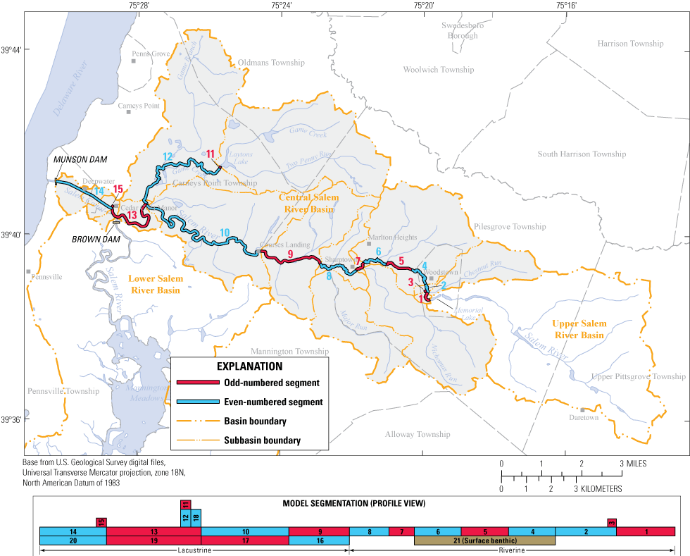
Map showing segmentation of the flow and eutrophication model of the central Salem River, New Jersey.
Table 3.
Segment information for the flow and eutrophication model of the central Salem River, New Jersey, 2007–08.[m, meters; --, not applicable; DAR, drainage-area ratio; LOADEST, load estimator program; PLOAD, geographic information system (GIS) pollutant loading application; WWTP, wastewater-treatment plant]
Named for location on or input/output to main stem Salem River, except segments 11 and 12, which represent Game Creek tributary.
Specified as the lowest depth in a segment before transport will cease. Used to keep segments from becoming dry or draining more than normal. (Wool and others, 2008)
The simulation period was designed to coincide with field data collection beginning April 1, 2007, and ending October 31, 2008. This period covers two growing seasons when the effects of eutrophication are greatest as a result of increased light, higher water temperatures, and an abundant supply of nutrients. Water year 2007 was slightly wetter than average (1940–2007), whereas water year 2008 was drier than average (1940–2008). The user does not control simulation time-step size in WASP version 7.3, but rather sets limits on the range of time-step size. To ensure representation of diurnal changes in DO concentration due to eutrophication, the maximum time step was capped at 240 minutes (min). Model output did not differ noticeably when the maximum time step was reduced to 15 min. WASP determines the optimal time step on the basis of discharge, so the simulated time-step range was 2.16–30.8 min, with a median of 15 min. The time interval of temporal model input (for example, boundary concentrations) ranged from hours to months, in part as a result of data availability. Linear interpolation was done by WASP between model-input values to match the selected time step.
Flow Model
Flow in the main stem of the central Salem River was simulated by using one-dimensional kinematic wave and ponded-weir overflow equations in WASP (Wool and Ambrose, 2006). Kinematic wave flow routing is a simple but realistic option to drive advective transport through free-flowing (riverine) segments. The kinematic wave equation calculates flow-wave propagation and resulting variations in flows, volumes, depths, and velocities resulting from variable upstream inflow. Two assumptions associated with the kinematic wave equation are (1) backwater effects (for example, an upstream rise in water surface as a result of downstream flow obstruction) are insignificant and (2) channel slope is moderate to steep. These assumptions are reasonable for riverine reaches above the confluence with Major Run (segments 1–8) where the potential for backwater effects from downstream impoundments is negligible, but not reasonable for lacustrine reaches below the confluence with Major Run (segments 9–20), where backwater effects are observed.
Advective transport through ponded (lacustrine) segments is controlled by a ponded weir overflow equation, which represents flow through ponded segments controlled by a downstream low-head dam or natural sill. This equation calculates outflow on the basis of water elevation above the weir. The very low slopes measured in lacustrine reaches were set to zero to activate ponded weir flow in WASP. Flow between upper and lower lacustrine segments (mixing) was controlled by vertical connectivity in the model. Flow through Munson Dam gates or leakage through Brown Dam flashboards could not be simulated because of model and data limitations. Simulation of flow through downstream dams could affect water-quality-model results in lacustrine segments. Flow-model inputs are discussed in detail below.
Data Needs
Input-data needs for the WASP flow model are separated into several categories. The following sections describe model inputs for channel characteristics, initial flows, and boundary flows. Some input data were collected or reported and some had to be estimated, as described below. The correspondence between these inputs and model segmentation is shown in table 3. Calibration-data needs for the WASP flow model include flows, velocity, and depth for the main-stem river.
Channel Characteristics
Model-segment lengths were obtained by using GIS software and a 2002 stream-delineation dataset (New Jersey Department of Environmental Protection, 2003b). Water-velocity, channel cross-sectional area, and water depth information were derived from streamflow measurements. (Channel depth can be computed from width and cross-sectional area.) Segment length, width, and depth ranged from 466 to 7,940 m (1,529 to 26,050 ft), 9 to 26 m (30 to 85 ft), and 0.1 to 0.87 m (0.33 to 2.85 ft), respectively. Half of total depth was used to separate upper and lower segments in lacustrine reaches; this division coincides approximately with the depth of stratification from measurements of water temperature and DO concentration. Precise field leveling was conducted in October 2008 from station 01482500 to station 01482580 to determine segment channel slopes, which ranged from 0.00009 to 0.002 (DePaul and Spitz, 2023). Manning’s roughness values for the main channel ranged from 0.04 to 0.05 as determined from standardized tables for stream channels of similar morphometry (Coon, 1998). This range is appropriate for natural winding streams with some weeds.
Initial Flows
Initial conditions for flow in the model were taken from flows estimated for April 1, 2007, as discussed in the next section. Because the effects of eutrophication are most extreme during the summer, which occurred a few months after the start of the simulation period, the effect of initial conditions on model results (model error) was expected and confirmed to be minimal.
Boundary Flows
Boundary conditions for the flow model were developed on the basis of flow at streamflow-gaging station Salem River at Woodstown (01482500), estimated flows for ungaged drainage (channeled and unchanneled) along the main stem, reported discharge from Woodstown WWTP, and reported diversion from Salem Canal. Boundary conditions are discussed in detail in the following sections.
Measured Flows
The only streamflow-gaging station in the study area is Salem River at Woodstown (01482500). Continuous flows at this station were used to define the upstream boundary condition of the model. Flow was recorded at 15-minute intervals and stored in the NWIS database (U.S. Geological Survey, 2022). Flow at this station varied from 0.022 to 36.3 cubic meters per second (m3/s) (0.072–119 cubic feet per second [ft3/s]) over the simulation period.
Estimated Flows
Ungaged flows to segments 2 and 4 through 14 were estimated by using the mathematical translation method, also known as the drainage-area-ratio method (Sauer, 2002, p. 81). Flows in lower lacustrine layers (segments 16–20) were not estimated but were accounted for by vertical mixing in the model, as discussed in later sections. The drainage-area-ratio method can be used to compute flows in ungaged subbasins on the basis of flows in comparable gaged subbasins (index station). The method is based on the high correlation between discharge and drainage area and is used to estimate flow at an ungaged site on the basis of the ratio of the ungaged drainage area to the gaged drainage area and gaged flow by using the following equation:
whereQsb
is discharge for subbasin,
Qindx
is discharge at index gage,
Asb
is drainage area for subbasin,
Aindx
is drainage area for index gage,
C1
is multiplicative coefficient,
C2
is additive (or subtractive) coefficient, and
C3
is exponential coefficient.
Choice of index gage for each ungaged subbasin was based on (1) proximity to the ungaged subbasin, (2) degree of similarity in land use between ungaged and gaged basins, (3) degree of flow regulation in the gaged basin, and (4) flow-calibration accuracy. The number of possible index gages was limited as a result of the small number of gaging stations in southwestern New Jersey. Gaging stations in Delaware also were considered but were deemed inappropriate on the basis of the selection criteria. Three gages were used as index gages: Salem River at Woodstown (01482500, drainage area 14.6 mi2), Maurice River at Norma (01411500, drainage area 112 mi2), and Raccoon Creek near Swedesboro (01477120, drainage area 26.9 mi2). Average flow per square mile ranged from 1.00 to 1.22 for these gages over the simulation period.
The drainage-area ratio between ungaged and gaged subbasins ranged from 0.02 to 0.53 for most subbasins in the study area. The ratio was smaller in a few cases reflecting the lack of adequate index gages with small drainage area. Estimated boundary flows from subbasins ranged from 0.003 to 16.34 m3/s (0.01–53.6 ft3/s).
Discharges and Diversions
Daily discharges from the Woodstown WWTP and Salem Canal diversion were obtained from reports provided by the facilities for the simulation period. Discharge flow averaged 0.014 m3/s (0.046 ft/s) and diversion flow averaged 0.464 m3/s (1.52 ft3/s) over the simulation period. Although discharge and diversion flow varied daily, the monthly flows varied little over the simulation period. Discharge is from model segment 3 and diversion is to model segment 15 (fig. 8).
Calibration
The goal of flow-model calibration is to determine the best fit between predicted and observed flows such that major flow processes are represented in the river. Because temporal measurements (observations) were available for streamflow, velocity, and depth, the model could be calibrated to all these variables, which provides additional verification that the model captures the range of flow conditions that may affect eutrophication processes. For example, water velocity affects transport of nutrients in streams and depth affects how much light can penetrate the water column and the degree of stratification that could affect eutrophication processes. Streamflow measurements were made at the time of water-quality sampling at locations represented by segments 2, 6, 7, 9, and 14. The first three segments are riverine reaches and the last two are lacustrine reaches. The simulation period extends from April 1, 2007, to October 31, 2008, but the focus of calibration was on the growing season each year. Most of the sampling was done during or close to summer; however, given the short period, the full period was calibrated rather than the season only. The flow model was calibrated initially on the basis of the flow data and then refined during water-quality-model calibration.
Goodness of fit between simulated results and observed data was evaluated by means of time-series graphs of continuous simulated flow, velocity, and depth versus discrete observed data. These graphs provided information about times when simulated results were over- or underpredicted, as well as the magnitude of the error. Goodness of fit also was examined by means of commonly used error statistics, including the means of observed and simulated values, root mean square error (RMSE), index of agreement (d), and percent bias (PBIAS). Error statistics may be of limited value because of the limited number of observations; thus, the graphs should take precedence in evaluating goodness of fit (all observed data, rather than a subset of the data, were used in computing error statistics). Equations for these metrics can be found in Moriasi and others (2015). RMSE is the standard deviation of prediction errors (residuals). Residuals are a measure of how far simulated and observed values are from the regression line, and therefore define the range of the error. The index of agreement is the ratio between mean square error and “potential error,” the latter of which represents the largest value the squared difference of each pair can attain. Index of agreement varies from 0 to 1.0, with higher values indicating closer agreement between simulated results and observations. Percent bias (PBIAS) is a measure of the average tendency of simulated values to be larger or smaller than observed counterparts; overprediction results in negative values and underprediction results in positive values of PBIAS. Additional information on the criteria for calibration assessment is discussed in the water-quality-model calibration section of this report.
Only hydraulic geometry (for example, channel depth and width), channel roughness, and estimated tributary watershed flows were adjusted to achieve the best fit between simulated and observed flow variables. Minor adjustments were made to hydraulic geometry because large changes adversely affected the accuracy of water-quality-model calibration. Segment length, channel slope, and initial flows were not adjusted. Estimated watershed flows for Chestnut Run and Game Creek were adjusted. Field inspection of Chestnut Run indicated little flow to the Salem River compared to estimated flows (0.01–0.91 m3/s [0.35–32.1 ft3/s]), indicating some of the flow could be diverted elsewhere. Although there were no data to support this assertion, several outflow pipes to the river were noted downstream from the confluence. Separation of the hydrograph into runoff and base-flow components for this tributary yielded base flows that far exceeded streamflows measured during water-quality sampling. Therefore, estimated flows for Chestnut Run were reduced by using a multiplier of 0.4 to achieve the best fit for flow and water quality calibration. Estimated flows for Game Creek (0.03–3.49 m3/s [1.06–123 ft3/s]) also were reduced by using a multiplier of 0.4 to achieve the best fit. This adjustment was used to account for simulating only the eastern fork of Game Creek and limitations of the modeling approach (for example, not simulating backwater or macrophytes). The following sections describe flow-model calibration in more detail.
Flow
Simulated hydrographs and flow measurements at the five calibration stations are shown in figure 9; associated error statistics are listed in table 4. Inspection of the graphs and error statistics indicates that the model simulates flow accurately in riverine segments 2, 6, and 7, but less accurately in lacustrine segments 9 and 14. Given that the weir outflow equation is an approximation used to simulate flow in lacustrine segments, calibration accuracy is expected to be less for these segments than for riverine segments simulated by using the more physically realistic kinematic wave equation. The weir outflow equation performs better for calibration of velocity and depth in lacustrine segments (presented in the next section), as simulated values more closely matched measured values.
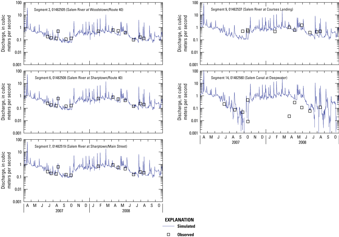
Graphs showing simulated and observed streamflow (discharge) in the central Salem River, New Jersey, 2007–08.
Table 4.
Calibration-error statistics for the flow model of the central Salem River, New Jersey, 2007–08.[Flow, in cubic meters per second; velocity, in meters per second; and depth, in meters]
Velocity and Depth
Simulated velocities were computed by dividing simulated flow by the simulated cross-sectional area for the appropriate model segment. Measured velocities were obtained from streamflow measurements. Calibrated results for velocity shown in figure 10 and error statistics listed in table 4 indicate a reasonable match. Simulated depths were a model output and measured depths were obtained from streamflow measurements. Calibrated results for depth shown in figure 11 and error statistics listed in table 4 also indicate a reasonable match. Percent bias indicated overestimation of velocity in riverine segments and index of agreement indicated a weaker match for depth in lacustrine segments than for riverine segments (table 4). Weaker matches for these variables did not correlate with weaker matches at the same locations in the water-quality model.
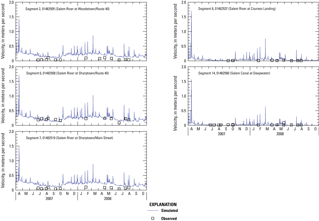
Graphs showing simulated and observed water velocity in the central Salem River, New Jersey, 2007–08.
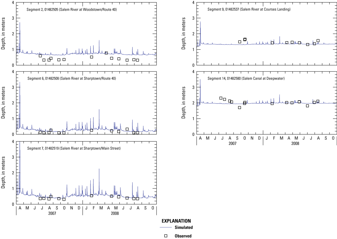
Graphs showing simulated and observed water depth in the central Salem River, New Jersey, 2007–08.
Transport and Residence Time
Advection and dispersion are major processes by which constituents are transported along and distributed throughout a river (Ji, 2008, p. 21). When the longitudinal dimension of a water body is large relative to its lateral dimension, lateral transport is considerably less important than longitudinal transport. Time-of-travel dye-tracer studies can be used to measure longitudinal transport. Time-of-travel data from unpublished dye-tracer studies conducted between Woodstown and 1.36 mi downstream from the Courses Landing Bridge on October 8–10, 1974 (DePaul and Spitz, 2023), were available to help assess transport. No calibration was done to match these data. Results of the dye-tracer study were compared to simulated results for the same reach during 2007–08, with the assumption that low-flow conditions were similar (less than 0.285 m3/s [10 ft3/s]), and measured time of travel (4.98 days) was comparable to simulated time of travel (4.69 days).
Water residence time can affect the amount of biological production in a water body. A water body that flushes rapidly (that is, the water has a short residence time) exports nutrients downstream rapidly, resulting in lower nutrient concentrations in the water body compared to a similar water body that flushes slowly. In addition, a water body whose flushing time is shorter than the doubling time of algal cells inhibits formation of blooms. On the basis of the calibrated model, average residence time in lacustrine segments of the Salem River was approximately 15 times longer than that in riverine segments. This simulated result supports the observation of large amounts of phytoplankton and macrophytes in lacustrine portions of the river.
Eutrophication Model
The advanced eutrophication module of WASP (Wool and others, 2003) was used to simulate water quality in the Salem River. Use of the module for this application simulates transport and transformation of 11 water-quality state variables in the water column. The model implements the one-dimensional finite-difference form of the mass-balance equation shown below. This equation includes the three major classes of water-quality processes: advective and dispersive transport, external loading, and transformation. Interactions between constituents are described by using first- and second-order chemical kinetics equations. The principal kinetics equations for dissolved oxygen and eutrophication are discussed in the WASP documentation (Wool and others, 2003). Units used in the equation are M for mass, L for length, and T for time.
wheret
is time [T],
A
is cross-sectional area [L2],
C
is concentration of the water-quality constituent [M/L3],
Ux
is longitudinal water velocity [L/T],
Ex
is longitudinal dispersion coefficient [L2/T],
SL
is direct and diffuse loading rate [M/T],
SB
is boundary loading rate (upstream, downstream, benthic, atmospheric) [M/L3T], and
SK
is total kinetic transformation rate (positive is source, negative is sink) [M/L3T].
The Salem River water-quality model uses the same water-column segments and simulation period as the flow model and uses the surface benthic layer beneath segments 4, 5, and 6 as a repository for local particle settling. The model solves for the concentration of each state variable for each segment. State variables include DO, CBOD (3 types), NH4, NO3, DON, DIP, DOP, inorganic solids, and phytoplankton CHL-a. Inorganic solids were simulated only to account for organic-nutrient sorption onto particles and settling from the water column but were not calibrated. CHL-a was simulated as a proxy for total phytoplankton population.
Because not every state variable was analyzed during monitoring, concentrations for some had to be estimated. As indicated above, total ammonia was assumed to equal ammonium as a result of the neutral to slightly alkaline pH of the Salem River and tributaries. DON was assumed to equal total Kjeldahl nitrogen (TKN) minus ammonia (NH4). DIP was assumed to equal filterable phosphorus because it composes most of soluble reactive phosphorus. DOP was assumed to equal the difference between TP and DIP. CBOD simulated in WASP represents CBODu, which was not analyzed. Therefore, 5-day CBOD data were converted to 20-day CBOD data on the basis of the computed decay rate from a limited number of concurrently collected samples and were used as a proxy for CBODu.
Data Needs
Input-data needs for the WASP water-quality model are separated into several categories. The following sections describe model inputs for initial concentrations, boundary concentrations and loads (nutrients, DO, CBOD, CHL-a), environmental parameters (segment parameters, time functions), vertical mixing (exchanges), and kinetic constants (biochemical reactions). Some input data were collected or reported and some were estimated, as described below. Table 3 describes the correspondence between some of these inputs and model segmentation. Calibration-data needs for the WASP water-quality model include constituent concentrations for the main-stem river.
Initial Concentrations
Initial concentrations for model constituents (other than nutrients) were set equal to or near boundary concentration values (discussed in next section) on April 1, 2007. Initial concentrations for nutrients at the upstream boundary were derived from the upstream boundary concentration files. Initial concentrations of nutrients for tributary watershed inputs to segments 2 and 4 through 14 were derived from estimated monthly loads (discussed in next section) and interpolated to account for shorter model “spin-up” time. The model “spin-up” process is used to generate a reasonable initial state from which the model can proceed. Initial concentrations for constituents in lacustrine bottom segments were set equal to concentrations in associated surface segments. Initial concentrations of nutrients for segment 3 (Woodstown WWTP) were set to observed or estimated values at the start of the simulation. Because the simulation began weeks before the growing season, it was assumed the effect of error in initial conditions dissipated prior to the growing season. Evaluation of model results verified this short-term effect.
Boundary Concentrations and Loads
Boundary concentrations and loads must be defined for each state variable at each model boundary (in contrast to initial concentrations, which are defined for all model segments), and the WASP user can choose to input values as one type or the other. If concentrations (in milligrams per liter) are used, WASP multiplies them by flows (in cubic meters per second) to compute loads at that boundary. If loads (in kilograms per day) are used, they are based on concentrations and flows at that boundary.
Nutrients
Nutrient inputs to the model are from nonpoint and point sources. The main nonpoint sources are associated with agriculture (fertilizer, manure), urban land uses, and atmospheric deposition. The main point source is the Woodstown WWTP. Nutrient boundary concentrations and loads were derived from a variety of sources for the Salem River model. Nutrient concentrations were used at segment 1 (upstream boundary) and segment 3 (Woodstown WWTP) primarily on the basis of measured data. Nutrient loads for tributary watersheds were estimated on the basis of relations between flow and land use because the data collected were insufficient for model input. Nutrient concentrations and loads are described in detail below.
Nonpoint Source
Boundary concentrations representing nutrient contributions from the upper Salem River Basin were input to model segment 1. Daily streamflow and discrete water-quality measurements from 2002–08 at the Woodstown station (01482500) were used to compute daily concentrations with regression equations developed by using S-LOADEST, a companion module to S-PLUS statistical software based on the LOADEST computer program by Runkel and others (2004). LOADEST relies on a seven-parameter log-linear regression model to develop relations between measured constituent concentrations and various functions of measured streamflow and seasonality parameters through use of the rating-curve method. S-LOADEST incorporates a maximum likelihood estimator (MLE) for uncensored data and an adjusted maximum likelihood estimator (AMLE) for censored data. In this study, censored data accounted for less than 2 percent of all data used in the regression models. Concentrations of NH4, NO3, DON, DIP, and DOP were regressed against streamflow over the full range of flows measured at Woodstown during 2002–08. The regression equations used to estimate nitrogen and phosphorus concentrations are listed in table 5.
Table 5.
Regression equations used in the development of nutrient loads and concentrations at station 01482500, Salem River at Woodstown, New Jersey.[R2, coefficient of determination; ln, natural logarithm; C, constituent concentration, in milligrams per liter; Q, centered streamflow, in cubic feet per second; sin, sine; cos, cosine; π, pi; dtime, centered decimal time]
PLOAD (U.S. Environmental Protection Agency, 2001), a simplified GIS-based model that estimates annual nutrient loads on the basis of each land-use class in a basin, was used to estimate nutrient loads from tributary watersheds to the central Salem River. Export coefficients, delineated subbasins, and land-use data were used in PLOAD to estimate these loads. Export coefficients represent the annual average total nutrient load to a system from a defined land use and are reported as mass of constituent per unit area per year. Export coefficients ideally should account for local variations in geology, soil type, and climate (Clesceri and others, 1986; McFarland and Hauck, 2001), and atmospheric deposition is assumed to be distributed uniformly and accounted for equally in each land-use class. Because stormflow was not sampled for the central Salem River, export coefficients were derived from storm-sampling data for the Lower Delaware River Watershed Management Area (WMA) (Baker and Esralew, 2010), Toms River Basin (Baker and Hunchak-Kariouk, 2006), and Upper Salem River Basin (Rutgers Cooperative Extension, 2012).
Data for 2002–07 from the Lower Delaware River WMA, which is physically, geologically, and hydrologically similar to the central Salem River Basin, was mainly used to develop export coefficients. Hydrograph analysis was performed for multiple storm events in six subbasins of the Lower Delaware WMA. Data from the Lower Delaware River WMA included discrete stage and streamflow measurements collected over a range of flow conditions. Rating curves developed from these data were used to estimate discharge from measured stage (continuous stage was measured only during storm events). Rating curves developed for all sites showed reliable correlations between stage and discharge (Baker and Esralew, 2010, p. 17); however, because data during the falling limb of each hydrograph were missing for most storms (fig. 12), it was necessary to extend each hydrograph in time to quantify the total discharge for each storm event (Baker and Esralew (2010, p. 19). Because stormflow diminishes exponentially through time, incremental discharges on the falling limb of the hydrograph can be estimated by using the equation in Gray (1970, p. 7.7). The time at which runoff ceases on the falling limb of the hydrograph can be estimated by using the equation in Linsley and others (1982, p. 210). Total discharge for each storm event can be estimated by integrating the volume under the curve.
Base flow during each storm event was approximated by drawing a line from the pre-storm minimum discharge to a post-storm discharge corresponding to the end of runoff or an actual base-flow measurement. Base-flow discharge during each storm event was then estimated by integrating the volume under the line. Runoff discharge during each storm event was computed as total discharge minus base-flow discharge. Because not all storms during the study period were sampled, total discharge, runoff, and base-flow components were scaled by dividing the volumes by the fraction of total precipitation represented by the sampled storms. Discharge volumes were then annualized by dividing by the number of years in each sampling period.
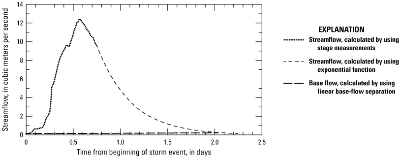
Hydrograph showing extension developed by using the exponential function method.
Event mean concentrations (EMCs) represent the mass of constituent per unit volume of water and were computed for each nutrient for each storm event; the resulting concentrations were averaged for all storms. EMCs were calculated for individual streams for growing and non-growing seasons as well as all seasons. Nutrient loads during runoff were computed by multiplying the EMCs for runoff samples by the annualized runoff volume. Yields (export coefficients) were derived by dividing the loads by the subbasin drainage areas.
Nutrient loads during base flow were computed by multiplying representative base-flow concentrations (BFCs) by the annualized base-flow volume. BFCs were determined for growing and nongrowing seasons from data collected within the Lower Delaware and Salem River (at Woodstown, Major Run, and Chestnut Run only) Basins and are assigned to the Salem River model subbasins on the basis of generalized land-use type (table 6). Where available, actual concentrations measured under low-flow conditions were used for tributary watersheds (Major and Chestnut Runs). Because Game Creek was included in the simulation and was not a boundary like other tributaries, low-flow concentrations were withheld and used for calibration and therefore could not be used in determining inputs. Base-flow loads were applied in segments 7 through 10 where base-flow indices were thought to be substantially greater than in other segments because of the presence of permeable sands rather than impermeable clays.
Table 6.
Nutrient concentrations in base flow used to calculate base-flow loads for general landscape types for growing and nongrowing seasons in the central Salem River Basin, New Jersey.[Values are in milligrams per liter; growing season is April 20 to October 20]
Returning to stormflow loads, because each of the drainage areas in which storm samples were collected contains a mix of land uses, the loading contribution of the major land-use classes needed to be isolated. Regression models were developed to relate annual loading rates (export coefficients) to major land-use classes. Emphasis was on determining export coefficients for agriculture because this is the dominant land use in the central Salem River Basin. The dependent variable in each regression model corresponded to the annual loading rate of the specific nutrient, and the independent variables corresponded to the fraction of each major land use. Dependent variables were adjusted by subtraction to account for other major land uses, such as the various types of urban land within each drainage area, as shown in equation 3 below.
wherei
is individual basins used in regression,
Yi(adjusted)
is annual loading rate of the targeted nutrient, acre,
Yi
is yield of the targeted nutrient at ith station/basin (pound/acre/year),
β2–4N
is nutrient export coefficient for various urban land uses (pound/acre/year), and
Xi,2–4
is fraction of various urban land uses within ith basin.
Values of export coefficients for urban land-use classes were derived from the literature because substantial work had been done on urban stormwater quality in the Upper Salem River Basin (Rutgers Cooperative Extension, 2012). Then Yi (adjusted) was substituted into a regression model of the form shown in equation 4 below.
whereβ0
is intercept, set to zero,
β1N
is nutrient export coefficient for agricultural land use (pound/acre/year),
Xi,1
is fraction of agricultural land use within ith basin, and
εi
is random error not explained in model peculiar to ith observation.
The regression models used a forced-zero intercept, which yields a zero load when all independent variables equal zero. The coefficients of each independent variable, if deemed statistically significant, represent the optimal export coefficient for those particular land uses (McFarland and Hauck, 2001). Export coefficients are input to PLOAD in pounds per acre per year (table 7), and loads are output from PLOAD in pounds per year, which are converted to kilograms per day for input to WASP.
Table 7.
Export coefficients used in the development of nonpoint-source loads of nutrients in the central Salem River Basin, New Jersey.[Values are in pounds per acre per year1]
Loads of NH4, NO3, DON, DIP, and DOP were estimated by using PLOAD for all tributary subbasins of the central Salem River. Land-use data were derived from a Watershed Management Area 17 digital dataset (New Jersey Department of Environmental Protection, 2007) and are shown in figure 3. Direct load calculation/interpolation based on water-quality samples from the upper Salem River Basin can be compared with PLOAD estimates. For example, the relative percent difference for NO3 loads is 26 percent, with PLOAD estimates being smaller. Although samples do not span the range of flow conditions during the collection period, this percent difference is likely less because PLOAD estimates account for runoff only, and not base flow.
Annual load values were apportioned monthly over the simulation period on the basis of observed long-term pattern of seasonal fluctuations in nutrients at the Woodstown station. A value representing the midpoint of each month was input to WASP, and values were interpolated automatically according to the time step. Finer time scale estimates (for example, in guidance by U.S. Environmental Protection Agency, 2007b) were not feasible with this model. Loads were used in the model at segments 2 and 4 through 14, but not at lower-layer segments 16 through 20 because of simulation of vertical mixing in the water column.
Point Source
Point sources in the Salem River Basin contribute only a small percentage of overall TP (3 percent) and TN (5 percent) loads compared to nonpoint sources. Woodstown WWTP effluent was used at model segment 3 as weekly nutrient loads based on reported data. Interpolation between values in kilograms per day was done automatically in WASP according to the time step. Discrete NH4 and TP concentrations obtained from both USGS sampling and reported by the facility (DePaul and Spitz, 2023) were used to estimate loads by multiplying concentrations by reported effluent flows. Because individual phosphorus species were not reported, it was not possible to calculate DIP and DOP concentrations. Because DIP is the dominant phosphorus species that remains after the wastewater treatment process (YSI Incorporated, 2021), a simple regression model based on USGS sampling data was used to estimate DIP concentrations from TP concentrations. DOP load was estimated by subtracting DIP load from TP load. NO3 and DON concentrations in effluent sampled by USGS were relatively constant over time, so concentrations were multiplied by reported effluent flows to estimate loads.
Dissolved Oxygen, Carbonaceous Biochemical Oxygen Demand, and Chlorophyll-a
Boundary concentrations for DO, CBOD, and phytoplankton CHL-a were required model inputs; these values were derived from several sources, as discussed below. Boundary concentrations for DO were set to measured values where data were available. Boundary concentrations for DO at segment 1 were incorporated as daily values based on observed data and results of two estimation methods used to fill the gaps. The first method was an empirical method derived by Weiss (1970) that describes equilibrium solubility of oxygen as a function of air pressure and water temperature. Application of this method matched DO concentrations measured during October to mid-May of 2007 and 2008 but underestimated those measured during the summer. The second method involved regression of measured DO concentrations into a continuous time series by using gaged flows at Woodstown (station 01482500) and time and seasonal parameters, as DO concentration is correlated with streamflow on a seasonal basis for the Salem River (Hunchak-Kariouk and others, 1999). Estimates based on regression more closely matched observed DO and were used as model input from mid-May to late September 2007 and mid-May to early August 2008. For tributary watershed inputs to the main-stem river, measured DO concentrations for Chestnut Run, Major Run, and Game Creek were input to segments 2, 8, and 12, respectively. For segments 4 through 7, 9 through 10, and 13 through 14 without data, an average DO concentration time series was used based on these three stations was used. DO concentrations from monthly NJPDES Discharge Monitoring Reports (New Jersey Department of Environmental Protection, 2009b) were used as input from the Woodstown WWTP.
Boundary concentrations for CBOD were divided into three compartments: CBOD1 in the river at the upstream boundary from the upper Salem River Basin, CBOD2 entering the river from tributary subbasins (segments 2, 4–10, and 12–14), and CBOD3 entering the river from WWTP effluent. This division results in greater flexibility in designing management scenarios by allowing for the tracking of different sources of CBOD. Also, 5-day CBOD concentrations were converted to 20-day CBOD concentrations as a proxy for CBODu concentrations. Decay-rate constants for Woodstown, Courses Landing, and Salem Canal were computed by using the method in Chapra (1997, p. 357) based on six 5-day CBOD analyses of samples collected concurrently with six 20-day CBOD analyses of samples (two samples per site). Boundary concentrations at segment 1 were based on 5-day CBOD analyses of samples collected at Woodstown and converted to CBODu concentrations by using the decay-rate constant for that site. For tributary watershed inputs to the main stem river, estimated CBODu concentrations for Chestnut Run, Major Run, and Game Creek were used for segments 2, 8, and 12, respectively. For segments 4 through 7, 9 through 10, and 13 through 14 without data, an average CBODu concentration time series was used based on these three stations. A 5-day/20-day CBOD ratio of 0.31 (Chapra, 1997, p. 357) was used to estimate CBODu concentration for the Woodstown WWTP.
Because eutrophication typically is a chronic and not an acute condition, CHL-a concentrations can be entered at a limited number of locations upstream from a critical location to “seed” the model. Therefore, boundary concentrations were used only where CHL-a analysis data were collected. Boundary concentrations for CHL-a at segment 1 were based on analyses of samples collected at Woodstown. Boundary concentrations for watershed inputs to the main-stem river were specified for the four tributary sampling sites: Chestnut Run (segment 2), Nichomus Run (segment 7), Major Run (segment 8), and Game Creek (segment 12). Inclusion of temporally variable concentrations at these few boundaries appeared appropriate on the basis of model results.
Environmental Parameters
Environmental parameters are model inputs composed of segment parameters and time functions. Segment parameters included water temperature (not simulated with temperature module), solar radiation, light extinction, SOD, benthic ammonia and phosphate fluxes, and settling rates for solids and phytoplankton. Time functions included water temperature, solar radiation, and benthic ammonia and phosphate fluxes. Time functions were set to vary diurnally or seasonally. Segment parameters vary spatially or are pointers to time functions. These pointers allow for both spatial and temporal variation of a segment parameter. Only segment parameters and time functions relevant to a particular simulation were used, which depends on data availability. Environmental parameters can be adjusted during model calibration. For example, light extinction, settling rate, and SOD benthic fluxes were adjusted to improve model results.
Water temperature is an environmental parameter that affects kinetic reaction rates. Three time functions were used to assign water temperature to water-column segments and were based on a daily water-temperature time series measured by DuPont Chambers Works (DePaul and Spitz, 2023) at Salem Canal (time function 3). Time functions 1 and 2 supplement this time series with limited finer scale data collected with multiparameter sondes during late summer 2008; time function 1 includes hourly data near Woodstown and time function 2 includes hourly (surface) data at Courses Landing. Time function 1 was assigned to model segments 1 through 8, time function 2 was assigned to segments 9 through 13 (and associated underlying segments), and time function 3 was assigned to segments 14 and 20. Model-input water temperatures based on these time series ranged from 3.9 °C in the winter to 30 °C in the summer, with a mean of 18–21.2 °C. Input water temperatures were varied spatially by using a segment parameter (for example, scale factors of 0.92 in riverine segments 4–8 and 0.92–0.97 in lower lacustrine segments 17–20) to account for riparian shading or deep water. Scale factors for lower lacustrine segments were estimated from vertical-profile sampling at Courses Landing and Salem Canal (fig. 6). Water-temperature measurements and the time functions agreed closely (fig. 13). Differences can occur as a result of differences in sampling location, tree canopy, flow velocity, and other conditions.
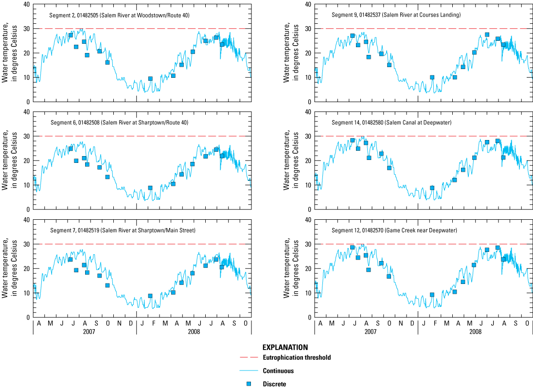
Graphs showing observed continuous and discrete water-temperature data in the central Salem River, New Jersey, 2007–08.
Solar radiation affects phytoplankton growth through photosynthesis during the day and respiration at night. Solar radiation was input to the model as a time function that applies to all segments. Solar radiation data were obtained from Northern Solid Waste Management Center in Wilmington, Delaware (University of Delaware, 2009), and were averaged on an hourly basis (fraction daily light set equal to 1). Values ranged from 1,824 Langley per day (Ly/d) during the day to 0 Ly/d at night, with a mean value of 338 Ly/d. Peak values were measured during June and July, with a mean value of approximately 475 Ly/d. Light attenuation (absorption) with depth in the water column was determined by using the Beer-Lambert equation in WASP (Wool and others, 2003), which includes a light-extinction coefficient. Light attenuation is caused by riparian canopy, water particles (background, CHL-a, dissolved organic carbon, solids), and other conditions. Light-extinction coefficient can be measured or estimated and is used as a segment parameter in the model. Because riverine reaches of the central Salem River are heavily canopied by trees, segments 1 through 8 were characterized by large light-extinction coefficients ranging from 8 to 17 per meter. Lacustrine reaches are much less canopied, so segments 9 through 14 were characterized by small light-extinction coefficients ranging from 0.8 to 2.5 per meter. These values are consistent with those used in other studies (Lung, 2001; Sullivan and others, 2006). Light-extinction coefficients were adjusted during model calibration to more accurately simulate diurnal variations in DO at Courses Landing.
Sediment diagenesis can be an important process in determining nutrient cycling and oxygen balance in the water column. Settling of nonliving phytoplankton and particulate nutrients (sorbed on inorganic suspended solids) in the water column can be an important source of nutrients to the sediment bed. Settled biomass and sorbed nutrients undergo biochemical reactions in the sediment bed, which can release nutrients back into the water column and create an oxygen demand on the water column. High concentrations of CHL-a, total suspended solids (TSS), TN, and TP at the upstream model boundary declined between segments 2 and 6. This decrease in concentrations can be accounted for by means of settling resulting from slow flow velocities. This process was included in the model by adding a surface benthic segment below water-column segments to represent a sink, as discussed previously. Also, the dissolved fraction of organic nitrogen and organic phosphorus was reduced in segments 4 through 6. Values were assumed because data on partitioning of these constituents in the water column were insufficient. The fractions were adjusted during calibration to increase the settling potential of high concentrations of these constituents in upper reaches of the model on the basis of loss or settling as indicated by observed data in these reaches. The dissolved fraction for CHL-a was set to 0 in all water-column segments according to guidance in the WASP manual (Wool and others, 2003). A settling rate of 0.07 m/d was applied for both phytoplankton and inorganic solids. Settling is important in reaches with reduced fluvial energy, and rates were based on lake or reservoir settling rates (for example, Ernst and Owens, 2009).
Benthic fluxes were applied in the model to account for SOD and nutrient exchange between the bottom sediment and water column. Two sources of SOD data were available: field measurements in the main-stem river at Sharptown and Courses Landing during summer 2008 (Heckathorn and Gibs, 2010), and laboratory measurements at five main-stem locations during summer and fall 1990 (Najarian Associates, 1990). Model input SOD ranged from 2 to 3.75 grams per meter squared per day (g/m2d) in riverine reaches and 2.3 to 5.5 g/m2d in lacustrine reaches. SOD values include adjustments made during model calibration to improve the simulation of diurnal DO variations at Courses Landing. These values are consistent with the limited observed data. Vertical-profile sampling at two lacustrine locations during the 2008 growing season indicated DIP and NH4 increased with depth in areas associated with stratification and anoxic conditions at the sediment/water column interface. These data are found in the NWIS database (U.S. Geological Survey, 2022). In the absence of benthic nutrient-flux data, this is sufficient evidence to indicate whether nitrate or iron reduction is occurring and whether inclusion of a benthic nutrient flux in the model is appropriate (DiToro, 2001). Therefore, model calibrated benthic flux in segments 16 through 20 during June–September ranged from 0 to 3.0 milligrams per square meter per day (mg/m2d) for DIP and 23.0 to 31.0 mg/m2d for NH4. Measurements from other studies conducted in freshwater (Kuwabara and others, 2009; Hammerschmidt and Mullen, 2016) indicate these ranges are reasonable.
Vertical Mixing
In addition to advective and dispersive transport, constituents are transported by vertical mixing. In the case of diffusion, concentration gradients cause constituents to move from locations of higher concentration to locations of lower concentration. Vertical mixing can be important in stratified, slow-moving water bodies as a result of gradients in water temperature, dissolved oxygen, etc. This process was included in the Salem River model by means of exchanges, which were applied between lacustrine upper and lower water-column segments. Vertical-profile data for water temperature and DO collected during summer 2008 at Courses Landing and Salem Canal indicated moderate to strong stratification, which appeared to persist throughout the summer. Monthly variations in thermocline diffusion coefficients were estimated by using equation 31.9 in Chapra (1997). Sub-weekly variations were estimated at Courses Landing to simulate DO variations at a finer scale. In the fall, turnover occurs as the result of the cooling of warmer surface waters, resulting in increased density, sinking, and displacement of some of the waters at the bottom, which are forced to rise and mix (Wetzel, 2001). Accordingly, the water column was simulated as fully mixed during nongrowing-season months, and a higher (than for growing season) constant value for exchanges was used. The range in values for vertical-diffusion coefficient was nearly an order of magnitude in the model.
Constants
The production or loss of a constituent, with or without interaction with another constituent, is a kinetic process that can be distinguished from a physical transport process or mixing. Reaction rates in WASP are simulated through chemical and biochemical kinetic constants. These rates affect reactions throughout the model and therefore are global parameters (constant in space and time), in contrast to environmental parameters discussed previously. Kinetic constants were input for several processes, including those related to nutrients, DO, CBOD, light, and phytoplankton. Initial values for constants in the Salem River model were based on ranges given in the WASP interface (Wool and others, 2003) or literature values (Bowie and others, 1985) used in other WASP eutrophication. Many of these constants were adjusted during model calibration; however, only those to which the model was sensitive are discussed in the calibration section below.
Calibration
Salem River water-quality model was calibrated by adjusting critical model inputs that affect phytoplankton dynamics, bioavailable nutrients, and dissolved oxygen. Calibration involved the manual adjustment of parameters through trial and error until simulated concentrations of model state variables closely matched observed concentrations at selected model segments. Monitoring data collected during 2007–08 were compared with model results. Approximately 10 discrete samples were collected per location, and limited continuous DO concentrations were measured at Sharptown and Courses Landing. The trial-and-error approach requires a conceptual understanding of the dynamics of the system, and determination of unknown or poorly constrained parameters can be difficult because they depend on complex physical and biochemical factors. Available data are typically inadequate to provide accurate estimates for these parameters. Also, because water-quality constituents interact with one another, improvement to calibration of one constituent at one location can worsen calibration of another constituent at another location, therefore requiring many simulations to achieve the best balance of results for all constituents at all locations given the final set of parameter values. Ultimately, calibration was based on a weight-of-evidence approach—that is, the best overall match for all constituents at all locations was chosen.
Model state variables for DO, CBOD, NH4, NO3, DON, DIP, DOP, and phytoplankton CHL-a were calibrated for the period April 1, 2007, to October 31, 2008. TN and TP concentrations computed by WASP were compared with observed concentrations to check overall mass balance of the system for nitrogen and phosphorus. Also, calibration of DON and DOP were considered secondary, as model skill is not typically assessed against estimated data. Calibration focused on matching observed data at six segments corresponding to sampling locations, including segments 2 (below Woodstown WWTP), 6 (Marlton Heights), 7 (Sharptown), 9 (Courses Landing), 12 (Game Creek), and 14 (Salem Canal). The first three segments represent riverine reaches, and the last three segments are lacustrine reaches. Emphasis in calibration was on the two growing seasons and diurnal DO concentrations at Courses Landing, a critical location (downstream site with the most historical monitoring data) for development of a TMDL (Helen Pang, N.J. Department of Environmental Protection, oral commun., 2012). The growing season is a critical time for eutrophic conditions to occur because sunlight, air temperature, and nutrient concentrations are all at a maximum.
Goodness of fit between simulated and observed concentrations was evaluated qualitatively by means of time-series graphs and quantitatively by means of error statistics. The same error statistics used for the flow model were used for the water-quality model. There are no best statistics to assess water-quality-model fit (Fitzpatrick, 2009; Engel and others, 2007; Wool, 2009), and the choice of statistic may affect the error; for example, R-squared has limitations related to bias and fit (Legates and McCabe, 1999). Although low values for error statistics may indicate the calibrated model does not account for all environmental processes that affect eutrophication, they may also reflect insufficient calibration data. Given a limited number of samples, error statistics are most appropriately applied to matching mean simulated and observed data for a defined time period (for example, weekly, monthly, or seasonal) rather than “point-to-point” comparisons. Therefore, because the water-quality data for this study are limited and kinetic constants are not well constrained, a goal of calibration was to reproduce the spatial and temporal distributions or trends in concentrations rather than to “curve-fit” the data. Also, the emphasis was on the graphs because the error statistics were less useful.
The main model inputs adjusted for water-quality-model calibration were kinetic constants, estimated watershed loads, selected environmental parameters, vertical mixing, and flow model parameters. Adjustment of kinetic constants was central to calibration, and final calibrated values are listed in table 8. Kinetic constants were constrained according to available data (for example, CBOD decay rate). During calibration of nitrogen and phosphorus concentrations, the nitrogen-to-phosphorus ratio was kept between 7:1 and 10:1 by weight to ensure that stoichiometric ratios required for algal growth (P:C, N:C, C:CHL-a) were preserved. Stoichiometric ratios can be adjusted during calibration because the nutrient composition of algal cells is not constant.
Table 8.
Calibrated global kinetic constants for the eutrophication model of the central Salem River, New Jersey, 2007–08.[--, not applicable; CBOD, carbonaceous biochemical oxygen demand; °C, degrees Celsius; mg/L, milligram/liter; SOD, sediment oxygen demand; ly, Langley]
Values of uncalibrated kinetic constants (not shown) remain at default values in WASP model interface (Wool and others, 2008). Refer to WASP model documentation (Wool and others, 2003) for additional information about individual constants.
Carbonaceous Biochemical Oxygen Demand
A goal of TMDL development for the central Salem River was to assess the effect of possible watershed-management actions on instream concentrations of DO. DO is a key indicator of eutrophication and of aquatic-system response. Potential sources of DO to the Salem River include reaeration at the water surface and algal photosynthesis. Reaeration was simulated in WASP by using the Covar method (Covar, 1976). This method shows how stream reaeration can be simulated using three formulas, each one of which is applicable in a different depth and velocity regime. Potential sinks of DO include CBOD (total), SOD, and algal respiration. All of these processes are represented in the model. Only CBOD and DO are model state variables that are calibrated.
CBOD concentration was calibrated mainly by adjusting the decay rate based on three sources described previously. Calibration graphs for CBOD concentrations are shown in figure 14 and error statistics are listed in table 9. For riverine reaches, simulated CBOD closely matched observed CBOD concentrations in segments 2, 6, and 7. For lacustrine reaches, the model underpredicted CBOD concentrations in segments 9, 12, and 14, possibly in part as a result of insufficient 20-day CBOD data, censored 5-day CBOD data, and inaccuracies related to CBOD sampling and analysis. Also, model hydraulic geometry does not fully capture local variations in lacustrine reaches, which are less channelized than riverine reaches, making flow/transport simulation less reliable. A large RMSE resulted for lacustrine surface segments, and PBIAS indicated underestimation in these segments (table 9).
Table 9.
Calibration-error statistics for the eutrophication model of the central Salem River, New Jersey, 2007–08.[Concentrations are in milligrams per liter, except for chlorophyll-a, which is in micrograms per liter; CBOD, carbonaceous biochemical oxygen demand; --, not applicable]
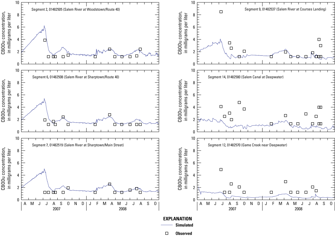
Graphs showing simulated and observed concentration of ultimate carbonaceous biochemical oxygen demand (CBODu) in the central Salem River, New Jersey, 2007–08.
Dissolved Oxygen
DO was calibrated by adjusting CBOD and SOD, and indirectly through calibration of nutrients and phytoplankton (discussed later). DO was sensitive to SOD but was not sensitive to CBOD, possibly because (1) CBOD consumption may be small compared with SOD consumption and (or) DO production (from a rapidly increasing phytoplankton population), (2) other kinetic reactions (for example, phytoplankton growth) may be faster than CBOD decay, and (or) (3) CBOD may account for a smaller percentage of total DO loss than other sinks. Vertical mixing between upper and lower model segments in lacustrine reaches also was adjusted until observed differences in vertical DO concentrations were reproduced.
Calibration graphs for DO concentrations are shown in figure 15, and error statistics are listed in table 9. Intensive sampling data collected during July–August 2018 at Courses Landing and Salem Canal are included in the figure. For riverine reaches, simulated DO closely matched observed DO in segments 6 and 7, but was slightly overpredicted in segment 2, which is near Woodstown WWTP. Simulated and observed DO concentrations varied widely in lacustrine reaches, which reflects greater eutrophication occurring in those reaches than in riverine reaches. Slower flow and reduced tree canopy in lacustrine reaches compared to riverine reaches make DO more sensitive to changes in solar radiation, increased air temperature, accumulation of organic matter, biological uptake (due to increased residence time), stratification, and sediment diagenesis. Despite the high variability, simulated concentrations approximated observed concentrations during the growing season in segment 9 (Courses Landing), whereas DO was slightly overpredicted in segment 12 (Game Creek) and slightly underpredicted in segment 14 (Salem Canal). A good visual match was achieved in bottom segment 20 (not shown), although the index of agreement indicated a weaker match in lacustrine bottom segments (table 9).
Simulated DO concentrations also were compared with continuous monitoring data at segment 7 (Sharptown) for July and August 2008 and at segments 9 and 16 (Courses Landing) for August to September 2008. Corresponding graphs are shown in figure 16 and error statistics are listed in table 9. For segment 7, DO is slightly overpredicted and simulated diurnal variations compare well with the observed diurnal variations, which reach 3 mg/L at Sharptown during algal blooms/peak productivity.
For segments 9 and 16, calibration was assessed on the basis of vertically averaged simulated and observed concentrations (fig. 16), which indicate a reasonable fit except for extremes. The segments were averaged because vertical discretization in the model was not refined. Alternatively, for surface segment 9 (not shown), simulated DO concentration was less variable and showed less frequent violations of the minimum surface-water-quality standard of 4.0 mg/L than shallow monitoring data; for bottom segment 16 (not shown), simulated DO concentration was less variable but better matched deep monitoring data. The reduced variability may be attributed to use of the monthly DO input concentrations as opposed to finer scale nutrient input loads and (or) simulating loads that are adjusted only to flow but not concentration. Reduced violations of the surface-water-quality standard may result from overpredicting reaeration and (or) not accounting for flushing of suboxic waters from wetlands along the main-stem river into the river during high-flow events. Diurnal variations in DO appear to be greater at Courses Landing than at Salem Canal, possibly because Courses Landing is the first lacustrine reach encountered by nutrients transported from upstream, photosynthetic activity and SOD potential is greater at Courses Landing as indicated by the presence of macrophytes in addition to phytoplankton, and (or) water releases through dam gates in Salem Canal.
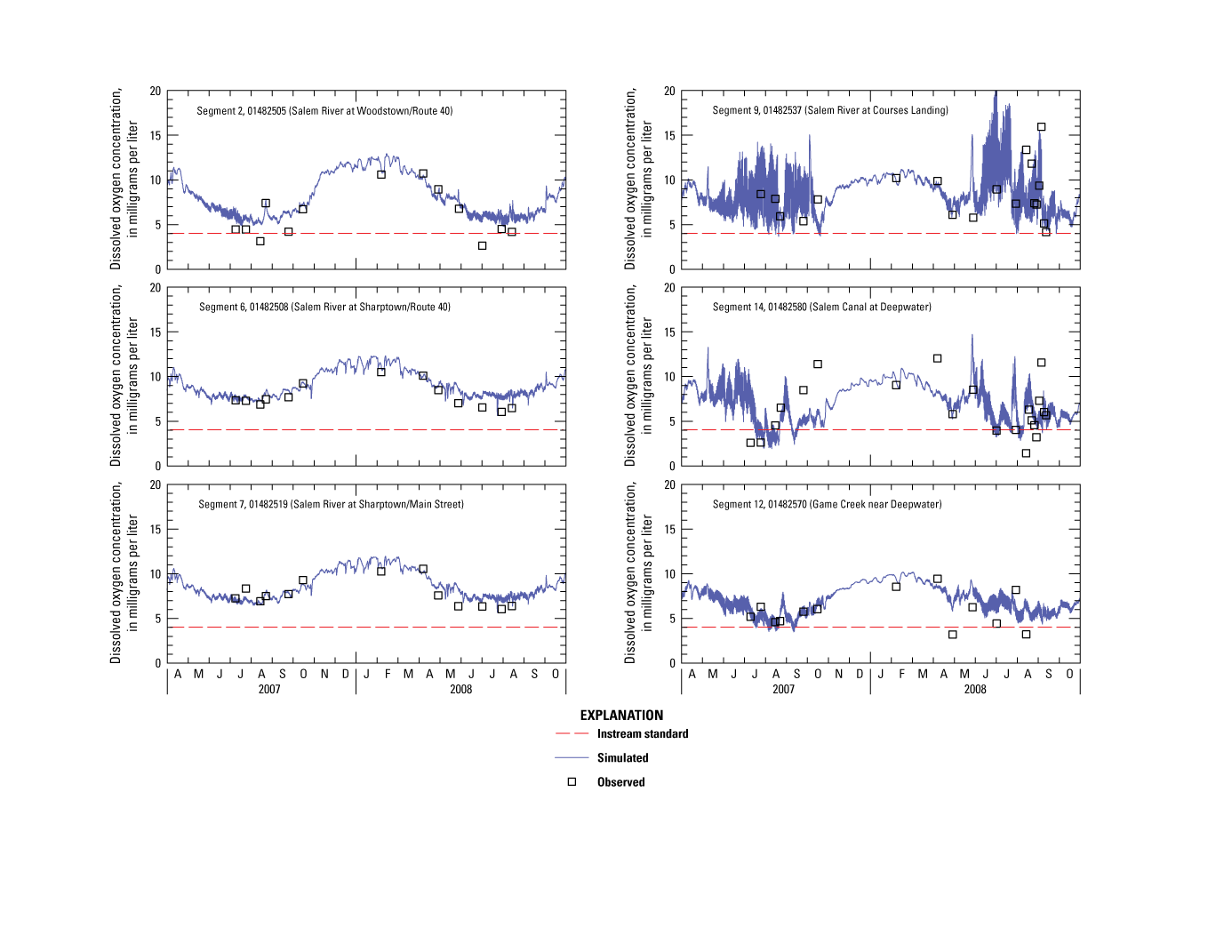
Graphs showing simulated and observed concentration of dissolved oxygen in the central Salem River, New Jersey, 2007–08.
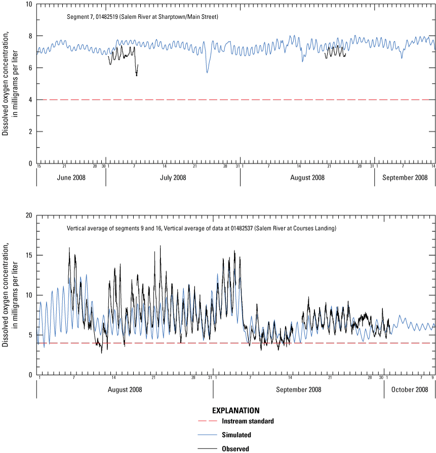
Graphs showing simulated and observed concentration of diurnal dissolved oxygen in the central Salem River, New Jersey, 2008.
Nitrogen
Potential sources of nitrogen that drive eutrophication in the Salem River include atmospheric deposition, nonpoint-source loads from agricultural activities, point-source loads from wastewater treatment, and release of nitrogen from river-bottom sediment. Atmospheric deposition is considered a minor source because the surface area of the river and tributaries that is exposed to the atmosphere is small. Potential sinks of nitrogen include uptake by aquatic plants including algae, which are simulated by WASP; however, macrophytes are not simulated. (Periphyton could be simulated by WASP, but no applicable data were available.)
Calibration graphs for NH4 are shown in figure 17, and error statistics are listed in table 9. Minor adjustment to input loads did not noticeably affect NH4 concentrations, which were calibrated mainly by adjusting the nitrification rate, DON mineralization rate, and phytoplankton growth rate. For riverine reaches, simulated NH4 concentrations closely matched measured concentrations in segment 2; however, NH4 was overpredicted in segments 6 and 7. Most of the observed data are near the simulated results, with the exception of a few high observed values. Matching storm peaks and diurnal variations is difficult without continuous or intensive discrete data. For lacustrine reaches, calibration was acceptable in segments 9, 12, and 14. PBIAS indicated overestimation of NH4 in riverine segments, and the index of agreement indicated a weak match for NH4 in lacustrine bottom segments (table 9).
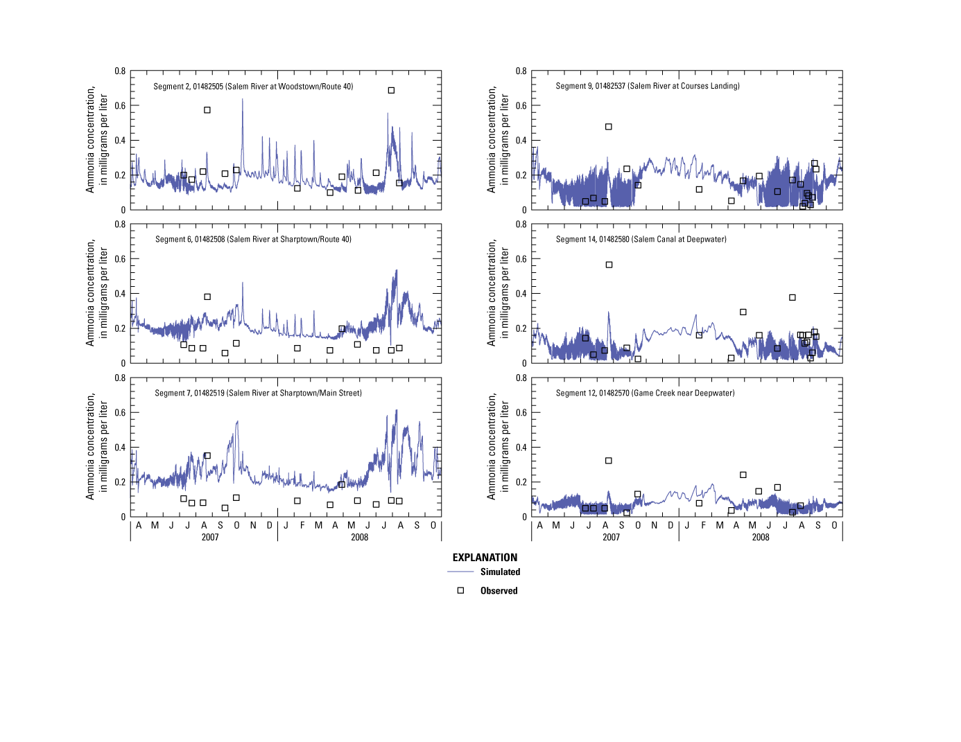
Graphs showing simulated and observed concentration of ammonia in the central Salem River, New Jersey, 2007–08.
Calibration graphs for NO3 are shown in figure 18, and error statistics are listed in table 9. Little adjustment was required during calibration of NO3 to produce a good fit between simulated and observed concentrations in all evaluated segments; the match was achieved after input loads were adjusted seasonally and nitrification rate was adjusted to balance NH4 and NO3 concentrations in the nitrification equation. NO3 concentrations during the simulation period were substantially less than the surface-water-quality standard of 10 mg/L. Extensive bordering wetlands, particularly in lacustrine reaches and the Game Creek watershed, may facilitate the removal of inorganic nitrogen through denitrification and, to a lesser degree, through assimilation by wetland plants.
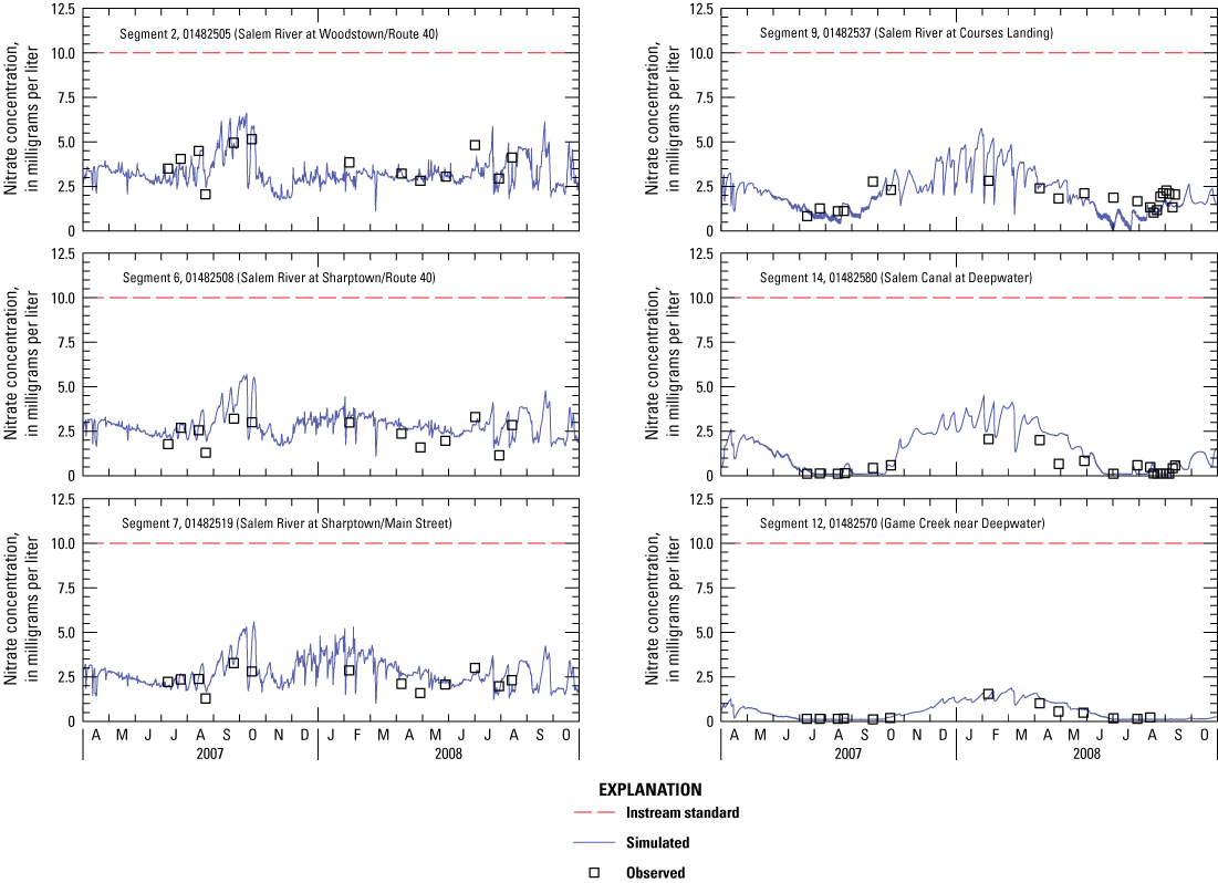
Graphs showing simulated and observed concentration of nitrate in the central Salem River, New Jersey, 2007–08.
Calibration graphs for DON are shown in figure 19, and error statistics are listed in table 9. DON was calibrated by adjusting input loads, uniformly scaling input boundary concentrations, altering DON mineralization rate, and adjusting the particulate fraction (PON) to be settled and settling velocity in the water column. For riverine reaches, simulated DON concentrations closely matched measured concentrations in segment 2 but were slightly overpredicted in segments 6 and 7. For lacustrine reaches, calibration was acceptable in segments 12 and 14, but simulated concentrations were slightly overpredicted in segment 9.
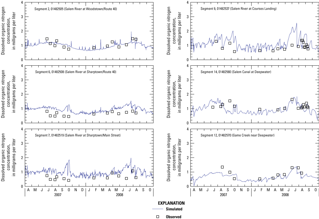
Graphs showing simulated and observed concentration of dissolved organic nitrogen in the central Salem River, New Jersey, 2007–08.
WASP computes TN as the sum of NH4, NO3, DON, and particulate nitrogen (PN). Good calibration of TN ensures nitrogen mass balance is achieved and depends on the accuracy of the calibration for nitrogen species. Calibration graphs for TN are shown in figure 20, and error statistics are listed in table 9. For riverine reaches, calibration was acceptable in segment 2, but simulated concentrations were slightly overpredicted in segments 6 and 7. Overprediction in segment 6 results from the cumulative overprediction of nitrogen species. For lacustrine reaches, calibration was acceptable in segment 12, but simulated concentrations were slightly overpredicted in segments 9 and 14.
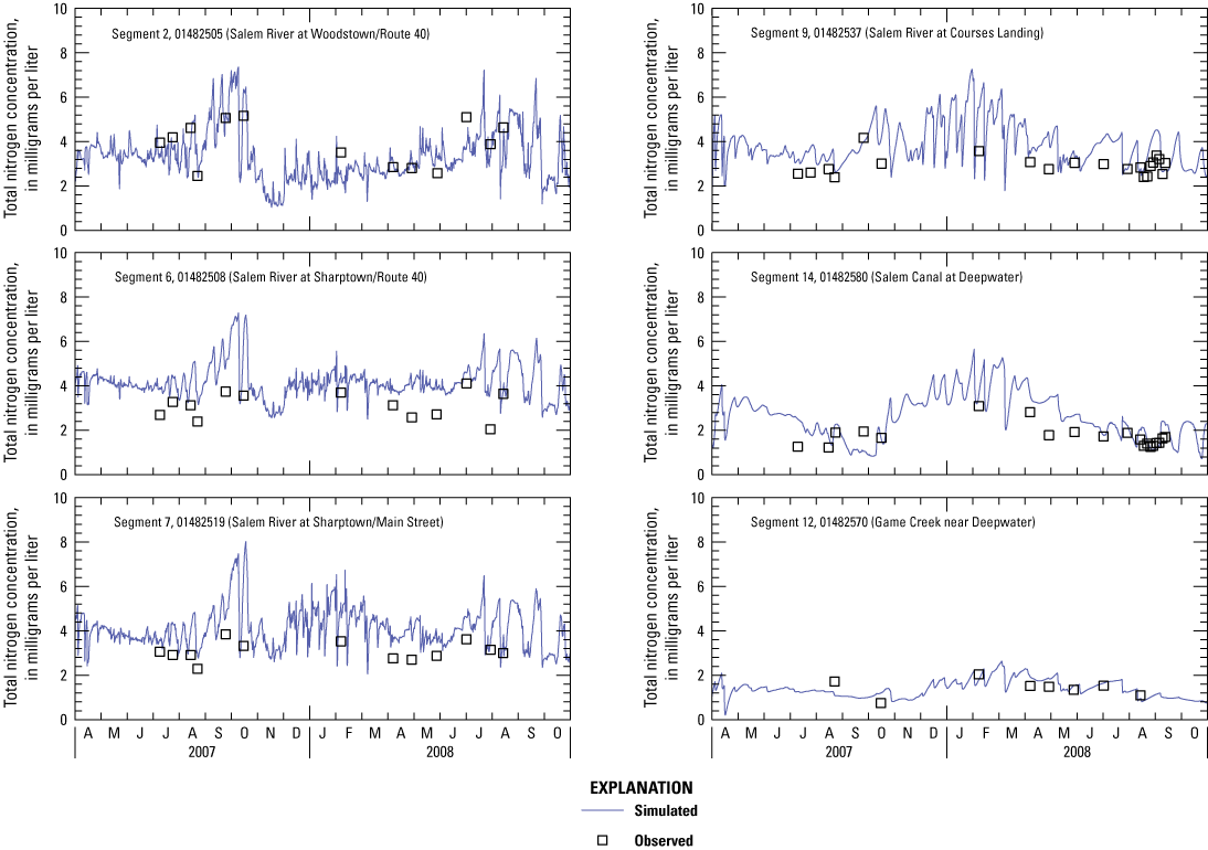
Graphs showing simulated and observed concentration of total nitrogen in the central Salem River, New Jersey, 2007–08.
Phosphorus
Potential sources of phosphorus in the Salem River include nonpoint-source loads from agricultural activities, point-source loads from wastewater treatment, and release of phosphorus from river-bottom sediment. Geologic formations that make up the Inner Coastal Plain contain phosphatic strata that may provide an additional source of phosphorus to the river through groundwater discharge (Sugarman, 1999; DePaul and Szabo, 2007). Potential sinks of phosphorus include uptake by aquatic plants, including algae.
Calibration graphs for DIP are shown in figure 21, and error statistics are listed in table 9. DIP was calibrated mainly by adjusting DOP mineralization rate and, to a lesser degree, by adjusting phytoplankton growth rate and phytoplankton stoichiometric ratios. Calibration was acceptable or slightly overpredicted in most model segments evaluated except in lacustrine segment 12, where simulated DIP concentration was overpredicted during the 2007 growing season. The inability to simulate retention of phosphorus in sediment behind Laytons Lake Dam and (or) not simulating Game Branch may account for the high simulated DIP concentrations in segment 12. The index of agreement indicated a weaker match for DIP in lacustrine segments than in riverine segments (table 9).
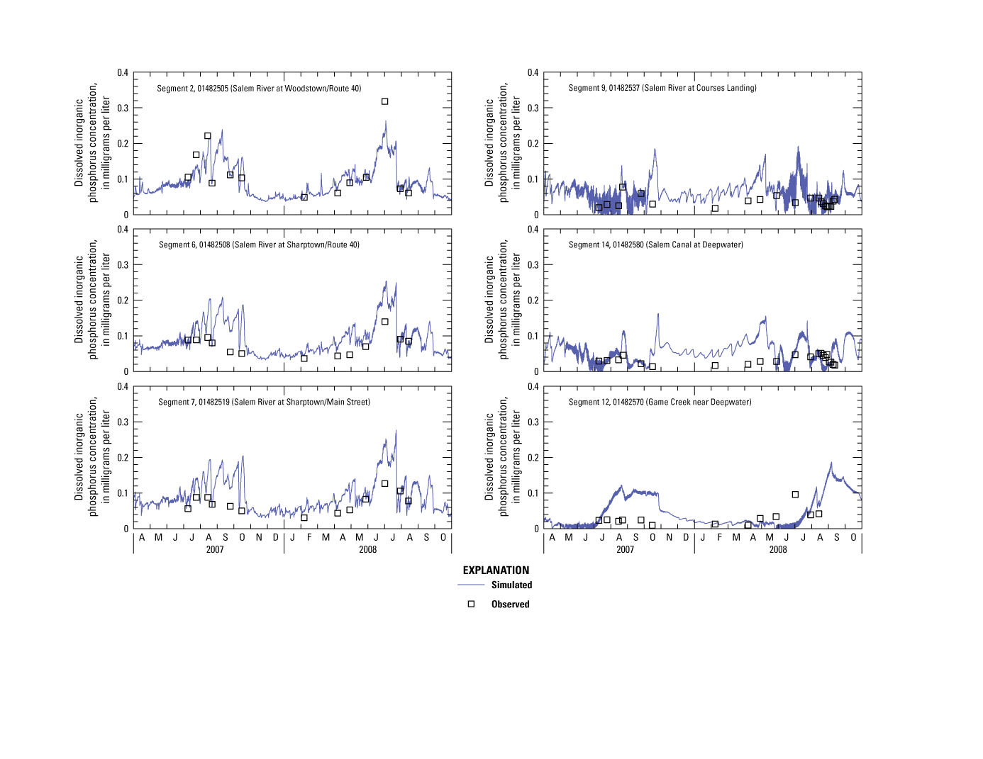
Graphs showing simulated and observed concentration of dissolved inorganic phosphorus in the central Salem River, New Jersey, 2007–08.
Calibration graphs for DOP are shown in figure 22, and error statistics are listed in table 9. DOP was calibrated by adjusting input loads, DOP mineralization rate, and particulate fraction (POP) to be settled and settling velocity in the water column. Watershed loads of DOP estimated by using the export coefficient approach generally were too high and therefore were reduced by almost 40 percent in segments 4 through 6 rather than by enhanced settling, which was deemed inappropriate given the lack of data. Watershed loads can overestimate delivery because (1) they lack temporal resolution, (2) associated ungaged flows may be overestimated, (3) export coefficients were derived from storm-sampling data collected in other watersheds, (4) no simulated attenuation or transformation processes occur during transport to the main-stem river and (5) DOP concentrations were computed rather than analytically derived. For riverine reaches, simulated DOP concentrations closely matched measured concentrations in segment 2 but were slightly overpredicted in segments 6 and 7. For lacustrine reaches, calibration was acceptable in segments 9 and 12, but simulated DOP concentrations were slightly underpredicted in segment 14. The index of agreement indicated a weaker match for DOP in riverine segments than in lacustrine segments (table 9).
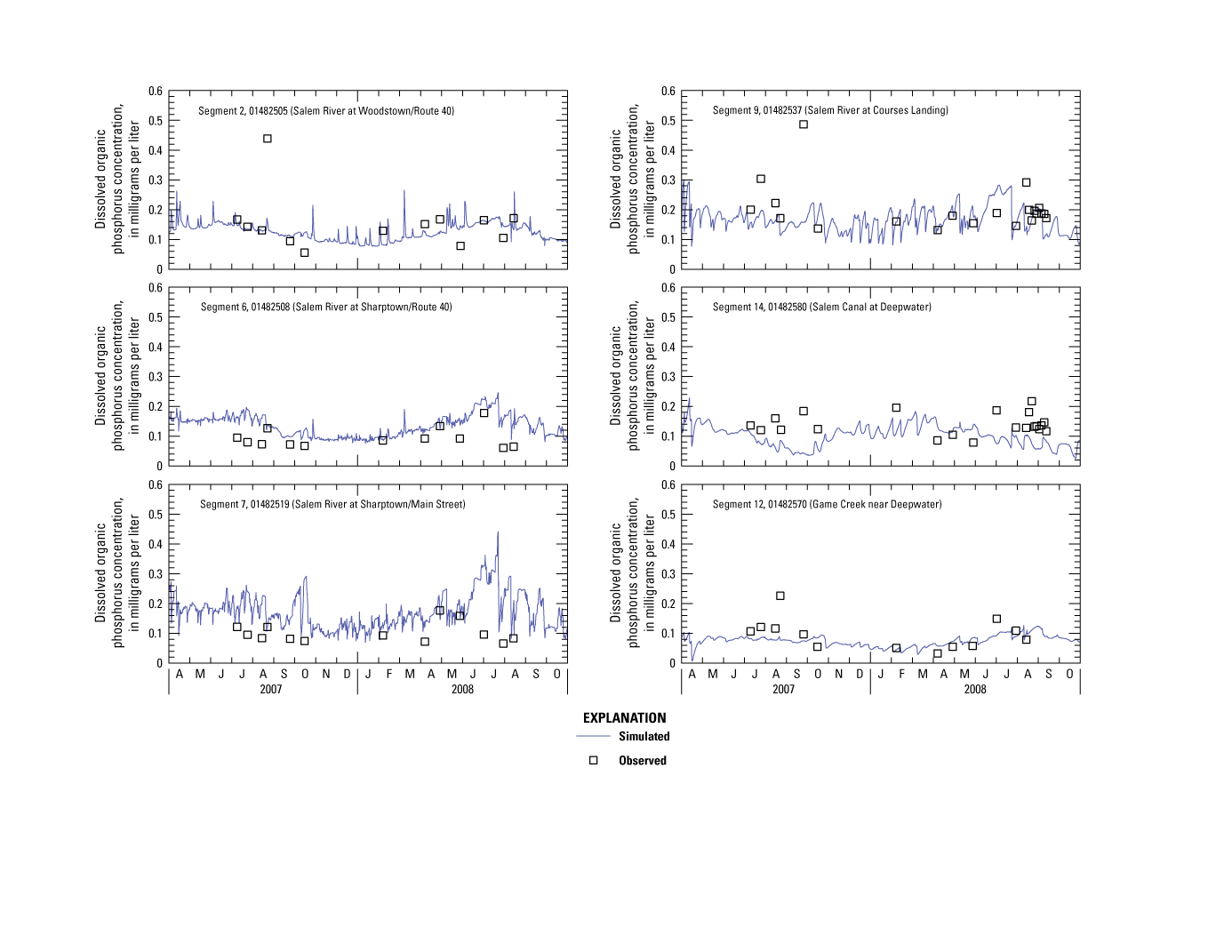
Graphs showing simulated and observed concentration of dissolved organic phosphorus in the central Salem River, New Jersey, 2007–08.
WASP computes TP as the sum of DIP, DOP, and particulate phosphorous (PP). Good calibration of TP ensures phosphorus mass balance is achieved and depends on the accuracy of the calibration for phosphorus species. Calibration graphs for TP are shown in figure 23 and error statistics are listed in table 9. For riverine reaches, calibration was acceptable in segment 2 but TP concentrations were slightly overpredicted in segments 6 and 7. For lacustrine reaches, calibration was in segments 9 and 14 but TP concentrations were slightly overpredicted in segment 12. The index of agreement indicated a weaker match for TP in lacustrine surface segments than in riverine segments (table 9).
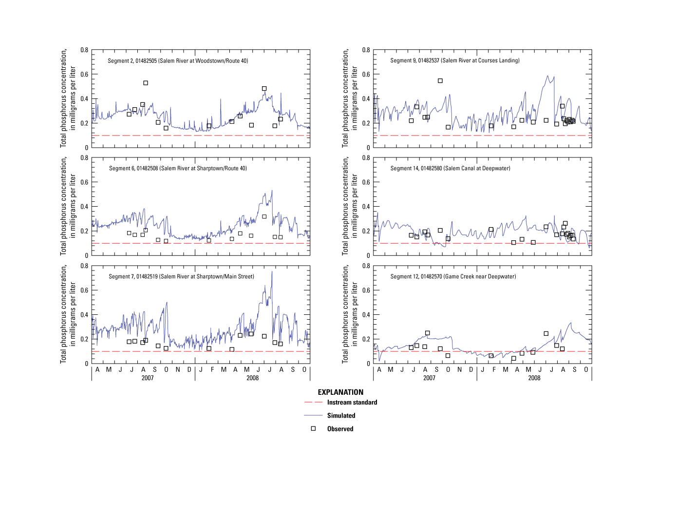
Graphs showing simulated and observed concentration of total phosphorus in the central Salem River, New Jersey, 2007–08.
Phytoplankton Chlorophyll-a
Algal growth is an aquatic-system response to environmental conditions described previously and is a key indicator of eutrophication. Another goal of TMDL development for the central Salem River was to assess the effect of possible watershed-management actions on instream concentrations of algae. CHL-a, a simple measure of algal biomass that is characteristic of all phytoplankton, was used as an aggregated state variable in WASP. Calibration of CHL-a for the Salem River model was achieved by uniformly scaling input boundary concentrations and adjusting kinetic constants such as stoichiometric ratios; phytoplankton growth, respiration, death, and recycle rates; and nutrient-uptake rates.
Calibration graphs for CHL-a are shown in figure 24, and error statistics are listed in table 9. Comparison of simulated and observed CHL-a concentrations indicate that the model generally matched overall trends in the algal population of the central Salem River. For riverine reaches, simulated CHL-a concentrations matched observed concentrations in segment 2 but were slightly overpredicted in segments 6 and 7. For lacustrine reaches, calibration was acceptable in segments 9 (except for the 2008 growing season), 12, and 14. Large RMSE were computed for riverine and lacustrine surface segments (table 9). A similar seasonal pattern was noted in simulated and observed CHL-a concentrations, with a decrease to a minimum during the winter months and an increase to a maximum during the mid- to late summer months. Simulated concentrations of CHL-a for the growing season, as well as for 2-week averages during the growing season, exceeded eutrophication thresholds of 24 and 32 µg/L, respectively, by as much as a factor of 4.
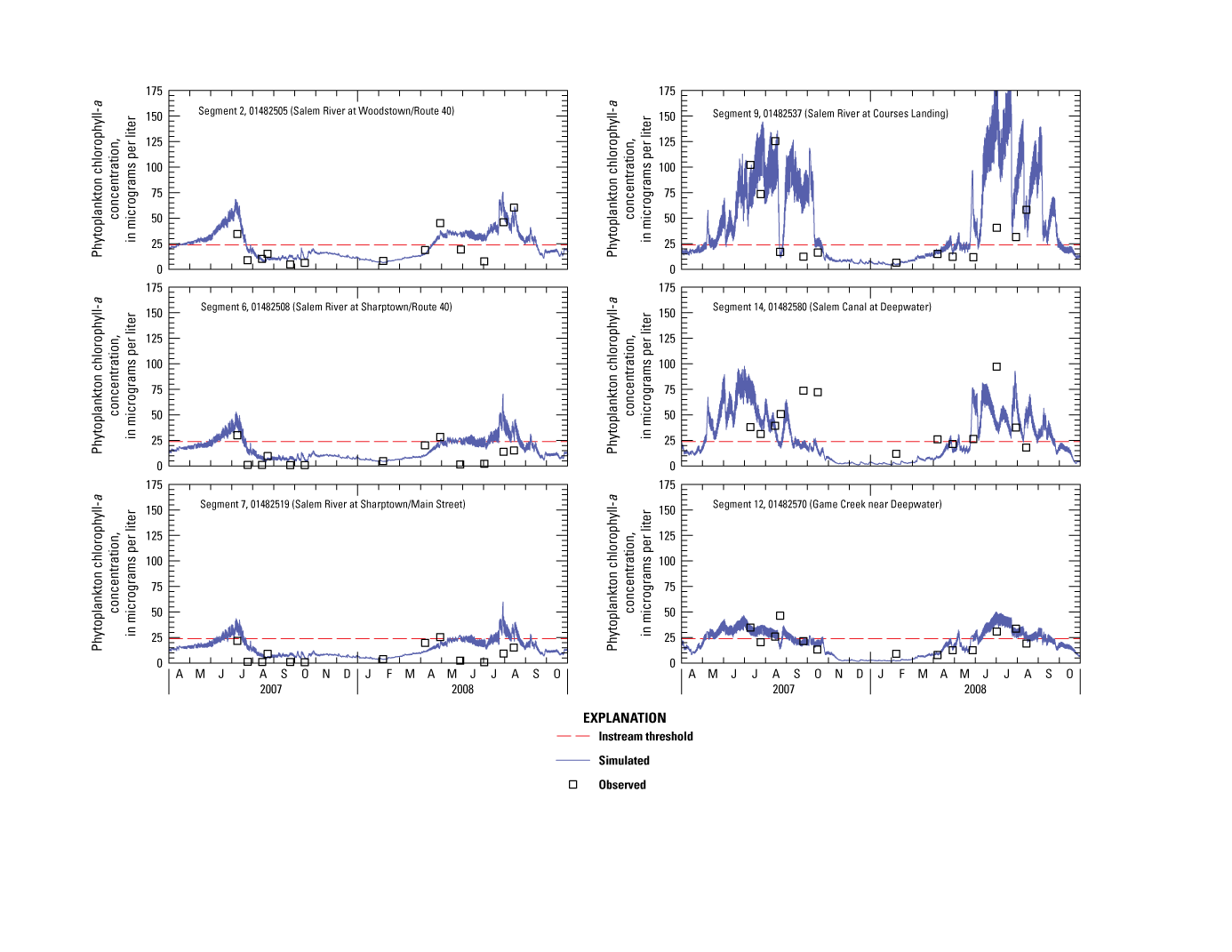
Graphs showing simulated and observed concentration of phytoplankton chlorophyll-a in the central Salem River, New Jersey, 2007–08.
The reason that some simulated values did not closely match observed concentration peaks, which involve substantial mass transfer (export from the basin during storm events), is not clear but may be explained by calibrated values for kinetics and (or) one or more of the following conditions: algal grouping, flow, water temperature, light, and nutrients. These factors are discussed in more detail below. Peak observed CHL-a concentrations may reflect the seasonal succession of phytoplankton species, whereby green and blue green algae, which are dominant in warmer air temperatures, are replaced by diatoms, which are dominant in cooler air temperatures (Ji, 2008). Because all phytoplankton species were grouped together and use one set of kinetic constants, individual species and their associated kinetics could not be represented. Extended hydrograph recession occurred in summer 2007, whereas several storm events occurred in summer 2008. Large volumes of flushing through downstream dams, which could not be simulated with the model, likely occurred during these storms. Water temperature input to the model was based on limited data at a daily time step. Use of more robust WASP light-extinction algorithms that account for algal self shading, background light extinction, solids, and dissolved organic carbon could improve the calibration if sufficient data are available. Similarly, more accurate tributary nutrient loads could be developed by using a watershed model.
Limitations on Algal Growth
About 16 times more nitrogen than phosphorus (or 7.2 times by weight) is required to produce a given amount of algae (Redfield, 1958). The practical range of this number is 10 to 20. A water body with a N/P ratio less than 10 may lack nitrogen for algal uptake, so nitrogen limits algal production. When the N/P ratio is greater than 20, the opposite may be true, and phosphorus becomes the potential limiting nutrient for phytoplankton growth. The molar ratio between nitrogen and phosphorus based on field data is referred to as the “Redfield ratio.”
WASP output provides information on nutrient and light limitations on algal growth. The simulated light limitation factor is based on the formulations of DiToro and others (1971) and Smith (1980). Examination of simulated output indicates that light is a critical limiting factor throughout the Salem River, particularly in riverine segments upstream from Courses Landing as a result of attenuation by dense tree canopy. That output indicates light is limiting throughout the system is not unexpected given that the Salem River is a nutrient-rich environment. The effect of nutrients on algal growth is shown in figure 25. Simulated growth on the left y-axis is associated with lines on the graph along which higher values represent less restricted growth conditions (nearer to 1) and lower values represent more restricted growth conditions (nearer to 0). The observed concentration ratio of DIN to DIP on the right y-axis is associated with points on the graph and is interpreted as the Redfield ratio.
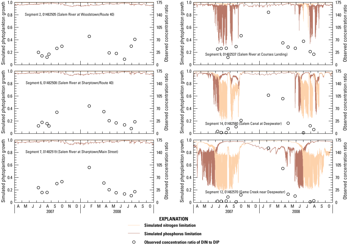
Graphs showing simulated nutrient limitation on phytoplankton growth and observed concentration ratio of dissolved inorganic nitrogen (DIN) to dissolved inorganic phosphorus (DIP), in the central Salem River, New Jersey, 2007–08.
WASP calculates nutrient limitation factors with the assumption that phytoplankton follow Monod growth kinetics with respect to phosphorus and nitrogen (Wool and others, 2003), whereby the growth rate is linearly proportional to nutrient concentrations at low levels (Ji, 2008). From a nutrient perspective, P is most commonly limiting in the main-stem river; however, nitrogen was limiting or colimiting in the Salem Canal during the summers of 2007 and 2008. Simulated results indicate only brief periods of N limitation at Courses Landing during June and July 2008, which is consistent with the concentration ratio of DIN to DIP derived from observed data. (If blue-green algae are nitrogen fixers in the summer, then this nitrogen limitation may be of less importance.) Both observed data and simulated results indicate the likelihood of a transition from P to N limitation in Game Creek during spring and summer in both years.
Model Sensitivity
A sensitivity analysis involves adjusting calibrated model parameters in a systematic way to determine which parameters have the greatest effect on model results. This exercise involves selecting a set of model parameters, varying each over a reasonable range, making perturbation model runs, and quantifying the effects on constituents critical to eutrophication. Model kinetics were the main parameters adjusted rather than other model inputs (for example, flow parameters, loads, vertical mixing), which were less easily varied. Two formal sensitivity analyses were conducted. The first sensitivity analysis was done prior to model calibration as a screening tool to guide parameter adjustments, whereby model response to individual parameter adjustments was not rigorously evaluated, but instead provided information on the primary driving forces in the system. Parameter values generally were limited to ranges suggested in the WASP interface or used in other WASP models. The model exhibited the greatest sensitivity to kinetics, in contrast to water-temperature correction factors and half-saturation constants.
The second sensitivity analysis was done after the model was calibrated. Selected input parameters were adjusted individually by using a 50-percent increase and decrease relative to the value in the calibrated model, and the model was run for each adjustment. Twenty-three model parameters were tested (table 10). Most adjusted values were within suggested ranges for WASP, if applicable, although two parameters, SOD theta and denitrification, were more than 20 percent outside the range. More than half of the parameter adjustments were to phytoplankton kinetics, about a third were to inorganic and organic nutrient kinetics, and the remainder were to oxygen demands and light.
Table 10.
Results of sensitivity analysis for the flow and eutrophication model of the central Salem River, New Jersey, 2007–08.[NSC, normalized sensitivity coefficient; °C, degrees Celsius; --, not applicable; m, meter; mg, milligram; P, phosphorus; C, carbon; N, nitrogen; Chl, chlorophyll; g, gram; Ly, langley; L, liter]
Model sensitivity was evaluated for DO, CBOD, NH4, NO3, DON, DIP, DOP, and CHL-a concentrations in surface (2, 6, 7, 9, 12, 14) and bottom (16, 18, 20) segments. Model results were evaluated by using two quantitative measures: percent sensitivity and normalized sensitivity coefficient. Percent sensitivity is computed as the average absolute percent change in residual between calibration-run results and sensitivity-run results. Normalized sensitivity coefficient is computed by using equation 5, as modified from Zhang and Rao (2012), and allows for the ranking of parameters that most greatly affect the model solution regardless of the direction of change:
whereNSC
is normalized sensitivity coefficient,
Θ0
is constituent value for the base (calibration) run variable,
P0
is parameter value for the base run, and
Θi and Pi
are values for the ith (perturbation) run.
Table 10 summarizes the results of the sensitivity analysis; it shows parameter sensitivity in descending order (from most to least sensitive). Model results indicate a wide range of changes in constituent concentrations in response to changes in input parameter values. Phytoplankton kinetics (growth, respiration, death), stoichiometric ratios, recycling of dead phytoplankton to organic nutrients, mineralization of organic nutrients to inorganic nutrients, and light extinction were the most sensitive parameters. Because of the close relation between phytoplankton dynamics and available nutrients, there is considerable overlap in critical parameters that affect algal biomass and those that affect nutrient dynamics.
DIP was the most sensitive constituent, followed by CHL-a, NH4, NO3, DOP, DO, CBOD, and DON. DIP was most affected by phytoplankton growth rate, P:C ratio, and recycle rate of OP. CHL-a was most affected by the phytoplankton growth rate, respiration rate, and death rate. NH4 was most affected by recycle rate of ON, phytoplankton growth rate, and light extinction. NO3 was most affected by phytoplankton growth rate, N:C ratio, and recycle rate of ON. DOP was most affected by phosphorus mineralization rate, recycle rate of OP, and P:C ratio. DO was most affected by SOD, SOD theta, and phytoplankton growth rate. CBOD was most affected by the CBOD decay rate, SOD, and SOD theta. DON was most affected by recycle rate of ON, N:C ratio, phytoplankton growth rate, and nitrogen mineralization rate.
Model Limitations
Water-quality models are complex and data intensive, requiring a large number of measurements related to spatiotemporal flows and concentrations, vertical stratification, benthic flux, landscape, climate, and artificial controls. The model code has inherent limitations. These limitations hinder the ability to match model results with observed data. It is important to understand the limitations of the Salem River model for proper interpretation of model results. Data and model limitations are described below followed by discussion to put these limitations in perspective.
Input and Calibration Data
The field dataset for the study was very limited. In terms of flow, data were not available on releases at downstream dams, which affects the accuracy of the ponded weir flow approach, as well as constituent transport and residence time behind the dams. Although stormwater sampling is important to capturing the effects of high flow on water quality, stormwater samples were not collected for this study, nor was sampling done during all seasons. As a result, it is not possible to verify that the model can accurately predict concentrations in all flow regimes and during the winter, although predictions during stormflows may be reasonable.
The limited availability of continuously recorded DO data makes it difficult to verify that the model can accurately predict the wide daily variations in DO concentration in lacustrine reaches of the river. The implications of this limitation are important because daily variation in DO concentration is a criteria in water-quality regulation. Limited oxygen-demand data, such as those for CBOD (and estimation of CBOD20 from CBOD5) make it difficult to evaluate the effect of this oxygen-removal process on DO concentration and compare it to the effect of SOD. CBOD is likely an important removal process in the river, and the magnitude of its effect may rival that of SOD.
Although SOD (benthic oxygen flux) was measured, the number of measurements was limited. Also, benthic nutrient fluxes were not measured or calculated. Therefore, it was necessary to simulate sediment diagenesis using descriptive input (specified fluxes) rather than predictive calculations (sediment diagenesis module). Flux data could be collected in order to better represent the sediment diagenesis component of nutrient recycling. The lack of constraint on model estimates may introduce uncertainty in model predictions. The magnitude of the effect of nutrient recycling due to benthic processes on eutrophication may rival that of tributary watershed inputs or surface runoff.
Because no sampling was done to determine particulate nutrient concentrations, nutrient data could not be partitioned into dissolved and particulate phases. Therefore, transport of particulate phosphorus and nitrogen could not be simulated in the model. Algal biomass varied widely among samples, which can affect the accuracy of calibration. Also, given the high sensitivity of the model to phytoplankton kinetics, identification of algal species could help with simulating more than one type of algae and defining their associated parameter ranges (for example, water-temperature parameters are different for diatom growth than for blue-green algae growth, and the half-saturation constant could be 0 for nitrogen-limited growth for nitrogen-fixing blue-green algae).
Estimated Data
The volume and chemistry of water introduced from some tributaries were not known and were approximated by using drainage-area ratio and export coefficients developed for nearby basins. These approximations may or may not represent actual conditions in the Salem River Basin. Using precipitation as a surrogate for streamflow results in overestimation of flow (and loads) because no water losses are accounted for, such as storage. Also, nutrient loads calculated with such methods do not fully account for attenuation or transformation during transfer. The load-estimation approach yields monthly values that cannot provide information about finer time-scale variations. Finally, using default values or values derived from literature for kinetic constants can introduce bias in model results if water-quality conditions in the study area differ substantially from those represented by default or literature values.
Model
The model is nonlinear and does not have a unique solution (that is, different combinations of input parameters will produce different results). For example, results of the flow model may have been improved by using a different configuration (such as routing flow in upper and lower lacustrine segments in addition to vertical flow between these segments), which also could have improved results of the water-quality model simulation. Similarly, water quality calibration of lacustrine segments could have considered averaged upper and lower segment concentrations.
Model results are affected by a short simulation period during which flow and water-quality conditions may not be representative of longer-term average conditions. For example, phosphorus in riverbed sediment in the Salem River likely is a persistent source resulting from tributary watershed inputs to the river and accumulated in the riverbed. Phosphorus is released back to the water column during low DO and (or) high-flow conditions (by means of scour and resuspension); this process will persist even for a time after watershed inputs have been removed (unless the channel is dredged or downstream dam gates are opened at regular intervals). If the simulation period had been longer, it may have been possible to evaluate this and related management actions.
WASP does not simulate certain eutrophication processes/transformations, such as those involving macrophytes. Other processes, such as erosion and deposition of sediments, could not be simulated in this study; a separate sediment-transport simulation and associated data collection would be required. The effect of such processes that could not be simulated on model results is unknown.
Discussion
Despite their limitations, water-quality models can be useful water-resource management tools. Although the lack of a comprehensive suite of data and estimates covering the full range of flow and water-quality conditions may yield inaccuracies in simulation and application results, the cost and time required to collect this information are typically prohibitive. A model may have inaccuracies with respect to short-term variations but may still capture the long-term trends of the system. Thus, the model can still be used to determine changes in the system and provide meaningful solutions to management questions (Ji, 2008). Models also can be used in an adaptive implementation or management framework (Loucks and van Beek, 2017), which allows for improvements in both the model and the data over time. Adaptive approaches strive to achieve water-quality standards while relying on monitoring and analysis to reduce uncertainty. This approach provides a way to move forward given the complexity of the real world compared to predictive models and the data available at the time a water-quality analysis is needed. Working with the data available and expanding data collection and model complexity as the need arises is a prudent approach.
Application of Model for Total Maximum Daily Load Development
The main goal of this study was to develop a water-quality model of the central Salem River that simulates flow, nutrient transport/cycling, and phytoplankton dynamics and can be used to test management simulations designed to improve water quality in the river. Close agreement between simulated and observed flows and constituent concentrations in the Salem River model indicates it reliably represents instream processes in response to environmental, meteorological, and loading conditions. Results from predictive simulations (scenarios) based on the calibrated model can help water-resource managers to establish TMDLs for concentrations of nutrients such as TP and receiving-water responses such as diurnal variations in concentrations of DO. Models are abstractions of reality and the complexity of predicting multiple state variables is constrained by model limitations, so the effects of these limitations need to be considered when interpreting scenario results. Further, the degree to which the model provides reliable constituent concentrations depends on whether the scenarios are fundamentally consistent with the calibrated flow and transport conditions that affect concentrations. Given the model does not have a unique solution, a scenario that invokes changes in flow or transport conditions may be of limited use.
Accordingly, two management scenarios were developed to reduce symptoms and effects of eutrophication in the Salem River by constraining the availability of nutrients from nonpoint sources along with upgrades in treatment at the Woodstown WWTP. The scenarios were developed in coordination with NJDEP, and other studies (for example, Wood and Rounds, 1998; Litke, 1999; Omni Environmental, 2007) were consulted regarding design and analysis for evaluating the effect of reduced nutrient loads on eutrophication. The model was first used to predict water quality under predevelopment conditions in order to identify stream reaches that might not attain water quality targets under natural conditions. The second scenario involves an extreme nutrient reduction; reduction amounts are constrained on the basis of simulation results for the previous scenario.
Results of the calibrated Salem River model for the simulation period (April 1, 2007–October 31, 2008) and growing seasons (April 20–October 20, 2007–08) provide baselines against which scenario results can be compared. These results were evaluated mainly for TP, CHL-a, DO, and TN at the same six locations (five main-stem river and one tributary) discussed previously in the calibration section. Courses Landing is of particular interest because it is a critical location—downstream site with the most historical monitoring data—for developing a TMDL (Helen Pang, N.J. Department of Environmental Protection, oral commun., 2012). Although segments 9 and 14 are surface segments with a corresponding bottom segment, results are presented for surface segments only in part because benthic fluxes were simulated by using descriptive input rather than predictive calculations.
Natural-Conditions Scenario
Design
The first scenario was designed to evaluate the effects of development on eutrophication in the central Salem River through a return to natural, predevelopment watershed conditions. Natural conditions impose the greatest limitations on algal growth compared to calibration conditions and represent a logical endpoint in load reductions. The general design of this scenario with respect to model boundaries is shown in table 11 and discussed below, although details of implementation in WASP are limited for brevity.
Table 11.
Design characteristics for the natural-conditions scenario.[TP, total phosphorus; TN, total nitrogen; mg/L, milligrams per liter; WWTP, wastewater-treatment plant; CHL-a, chlorophyll-a; SOD, sediment oxygen demand]
TP concentration at Memorial Lake was reduced and capped at 0.05 mg/L, with DIP or DOP species reduced by the same percentage and not preferentially. TN concentration was not reduced at the Memorial Lake boundary. Natural load conditions for watershed runoff and base flow were based on nutrient export coefficients and base-flow concentration equivalents, respectively, that were assumed to best represent unaffected (predevelopment) land uses in the study area. Urban and agricultural lands in the central Salem River Basin were treated as undeveloped forest land and assigned an appropriate nutrient export coefficient based on values for Gravelly Run subbasin, a pristine subbasin in neighboring Cumberland County (Baker and Esralew, 2010). (The Gravelly Run subbasin is outside the Inner New Jersey Coastal Plain and is not necessarily representative of those subbasins.) Similarly, base flow and base-flow concentration equivalents from predominantly undeveloped subbasins during the growing and nongrowing seasons were assigned to subbasins entering main-stem reaches that were assumed to be gaining, based on water-table contours and general surficial geology (for example, transmissive sands versus clays beneath river channel), to estimate natural base-flow load. Also, reduced runoff and the associated increase in base flow that would be expected to occur under natural conditions were not accounted for and are a limitation of the scenario design.
Other model boundary conditions, including CHL-a concentrations and oxygen demands, were modified to reflect natural conditions. CHL-a was reduced on the basis of reduced TP concentrations by using the regression relation established between these parameters for the extreme-nutrient-reduction scenario. Similarly, SOD was reduced on the basis of reduced TP concentrations by using the regression relation established between these parameters for the extreme-nutrient-reduction scenario. CBOD was another oxygen demand that could be reduced, but given that the largest input of CBOD to the Salem River is Woodstown WWTP, removal of this input in the scenario design best represented the lower CBOD associated with natural conditions.
Simulation Results
Phosphorus
Simulated results for TP for calibrated conditions and the natural-conditions scenario are listed in table 12 and shown in figure 26. TP concentrations exceeded the 0.1-mg/L surface-water-quality standard during much of the study period for calibration conditions. Under the natural-conditions scenario, average TP concentrations decreased by 82 to 85 percent during the growing season and were less than the surface-water-quality standard of 0.1 mg/L during the entire simulation period. A decrease in DIP concentrations during the growing season (not shown) is similar to that for TP concentrations; however, the percent change in DIP concentrations between calibration and the scenario simulation was much larger as a result of removing the point-source discharge representing the Woodstown WWTP, which is a major source of DIP.
Table 12.
Constituent concentrations under calibration conditions and natural-conditions and extreme-nutrient-reduction scenarios, central Salem River, New Jersey, 2007–08.[Concentrations in mg/L (milligrams per liter) or μg/L (micrograms per liter); >, greater than; <, less than; bold indicates concentration that violates water-quality standard or threshold]
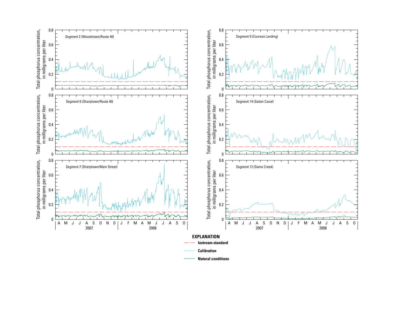
Graphs showing simulated concentration of total phosphorus for calibration and natural-conditions scenario, central Salem River, New Jersey, 2007–08.
Phytoplankton Chlorophyll-a
Simulated results for CHL-a for calibrated conditions and the natural-conditions scenario are listed in table 12 and shown in figure 27. CHL-a concentrations exceeded the 24-μg/L eutrophication threshold in segments 2, 9, 12, and 14 during most of the growing season for calibration conditions, whereas the threshold was exceeded in segments 6 and 7 for shorter periods. Under the natural-conditions scenario, average CHL-a concentrations decreased 81 to 90 percent during the growing season and were much lower than the threshold, except briefly in segment 9 during 2008. Also, the diurnal variation in concentration in lacustrine segments (9, 12, 14) was much smaller during the growing season than for calibration conditions.
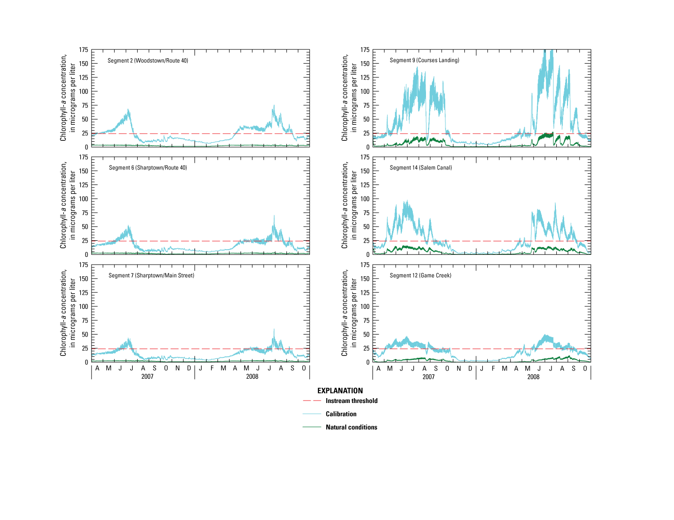
Graphs showing simulated concentration of chlorophyll-a for calibration and natural-conditions scenario, central Salem River, New Jersey, 2007–08.
Dissolved Oxygen
Simulated results for DO for calibrated conditions and the natural-conditions scenario are listed in table 12 and shown in figure 28. Only in segment 14 and intermittently in segments 9 and 12 were DO concentrations less than the minimum surface-water-quality standard of 4.0 mg/L during the growing season for calibration conditions. The daily average DO concentration often exceeded the standard of 5.0 mg/L in all segments during the growing season for calibration conditions. The maximum daily variation in DO concentration was greater than the 3-mg/L guidance level in segments 9 and 14 during the growing season for calibration conditions.
Under the natural-conditions scenario, all minimum DO concentrations were higher than the minimum 4.0-mg/L standard and ranged from 4 to 145 percent higher than for calibration conditions during the growing season. The daily average DO concentration exceeded the standard of 5.0 mg/L in all segments during the growing season. The maximum daily variation in DO concentration decreased as much as 86 percent and was less than the 3-mg/L guidance level in all segments during the growing season. No violation of DO surface-water-quality standards occurred, including for bottom segment 16 (not shown), although an unintended consequence was lower daily average DO concentrations resulting from reduced photosynthesis.
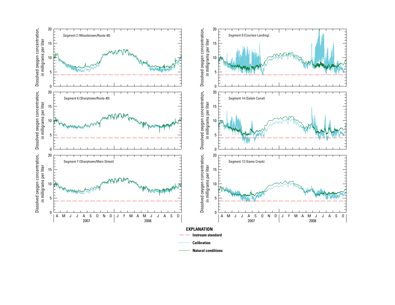
Graphs showing simulated concentration of dissolved oxygen for calibration and natural-conditions scenario, central Salem River, New Jersey, 2007–08.
Nitrogen
Simulated results for TN for calibrated conditions and the natural-conditions scenario are shown figure 29. Comparisons are not included in table 12 as a result of the small reduction in nitrogen in the scenario design. Under the natural-conditions scenario, TN concentrations in all segments were much lower than under calibration conditions, mainly as a result of removing the WWTP load and the accompanying reduction in watershed loads.
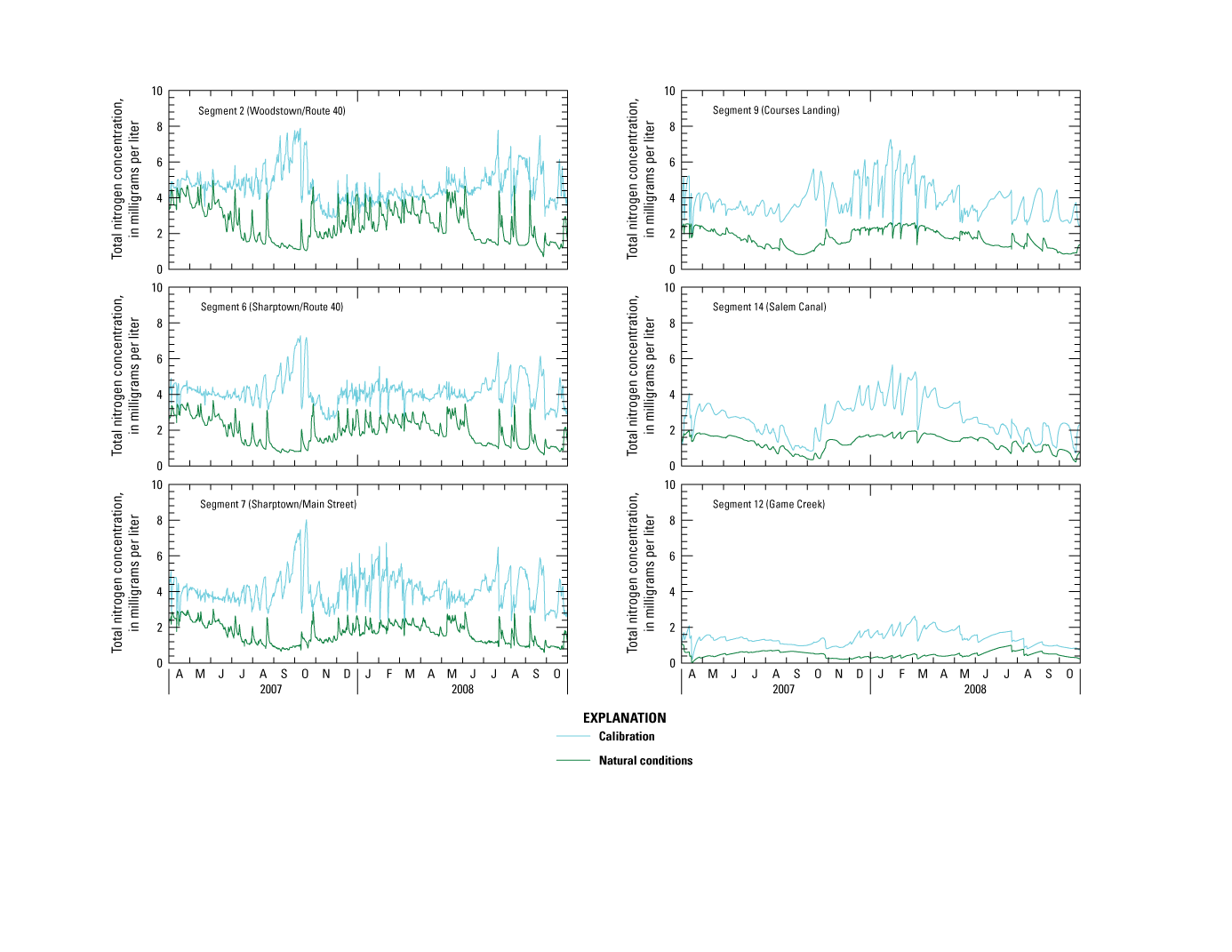
Graphs showing simulated concentration of total nitrogen for calibration and natural-conditions scenario, central Salem River, New Jersey, 2007–08.
In segment 2, NO3 concentrations (not shown) for the natural-conditions scenario were much lower than those under calibration conditions, whereas NH4 concentrations (not shown) changed little, indicating the upper Salem River Basin likely is a primary source of NH4 to the central Salem River Basin. NO3 and NH4 concentrations were lower in segments 6, 7, and 9 during the growing season as a result of load reductions. In segments 12 and 14, NO3 concentrations increased for short periods during the growing season, possibly as a result of decreased algal productivity and the associated decrease in NO3 assimilation during photosynthesis. The diurnal variation in NH4 concentrations decreased in lacustrine segments, indicating reduced photosynthesis resulting from reduced phytoplankton. The surface-water-quality standard for NO3 of 10 mg/L was not exceeded under calibration conditions or in the natural-conditions scenario.
Extreme-Nutrient-Reduction Scenario
Design
This scenario represents an extreme reduction of nutrient loads in the central Salem River Basin. The general design of this scenario with respect to model boundaries is shown in table 13 and discussed below, although details of implementation in WASP are limited for brevity.
Table 13.
Design characteristics for the extreme-nutrient-reduction scenario.[TP, total phosphorus; TN, total nitrogen; mg/L, milligrams per liter; WWTP, wastewater treatment plant; DIP, dissolved inorganic phosphorus; DOP, dissolved organic phosphorus; CBOD, carbonaceous biochemical oxygen demand; Mgal/d, million gallons per day; CHL-a, chlorophyll-a; SOD, sediment oxygen demand]
A cap of 0.05 mg/L on TP concentration at Memorial Lake is equivalent to a 72-percent reduction in this parameter from the upper Salem River Basin. TP reductions at this location were not allocated preferentially to either DIP or DOP; each species was reduced by the same percentage. However, a DIP:DOP ratio of 1:9 was applied to the Woodstown WWTP effluent to account for the preferential removal of inorganic phosphorus during tertiary wastewater treatment. Also, as the reduction in phosphorus at the Woodstown WWTP was based on the maximum permitted flow, flow was set to this value in the corresponding model segment. However, permitting guidelines for phosphorus discharge (State of New Jersey, 2008) were not considered in the design. Watershed runoff loads for TP and TN were reduced as indicated in table 13, and corresponding base-flow loads were reduced by small percentages as determined from the regression relations.
A positive relation between summer phytoplankton CHL-a concentration and TP concentration for temperate lakes and some flowing waters is well established in the literature (Wetzel, 2001). This relation also is evident in water-quality data for the Salem River tributaries. Therefore, CHL-a concentrations at model boundaries were reduced relative to reduced phosphorus loads by using a linear relation between the two constituents. The cap on TP load at Memorial Lake is equivalent to an 80-percent reduction in CHL-a concentration at this location. At low levels of TP (≤0.04 mg/L), a relation could not be determined from available data or from data from nearby basins; however, CHL-a concentrations computed on the basis of the regression were within the range of observed data at Crosswicks Creek, which drains a predominantly undeveloped basin in the Inner Coastal Plain of central New Jersey, including the central Salem River Basin. CHL-a concentrations were adjusted further to account for the difference between the growing and nongrowing seasons: ratios were determined on the basis of observed CHL-a data at five sampling stations (Memorial Lake, Chestnut Run, Nichomus Run, Major Run, and Game Creek), and each ratio was used to estimate nongrowing-season concentrations at each station.
Although reduced phosphorus loads to the river would result in reduced CBOD, available field data were insufficient to develop a relation between these two variables, and an appropriate literature reference could not be found. Model sensitivity analysis indicated that an order-of-magnitude reduction in CBOD had little effect on DO concentration. Therefore, only reductions in CBOD associated with reductions in phosphorus in the Woodstown WWTP effluent were simulated. The difference in CBOD concentrations between influent and effluent at the Woodstown WWTP indicated 99-percent removal through secondary treatment. To account for an upgrade to tertiary treatment as part of this scenario design, effluent CBOD concentrations were reduced by 30 percent on the basis of guidelines for advanced wastewater treatment designed to achieve low concentration of phosphorus (U.S. Environmental Protection Agency, 2007a).
SOD is an important factor affecting DO concentrations in the river, particularly in slow-moving lacustrine reaches. Reduced phosphorus loads to the river would likely cause reduced SOD in riverbed sediments, although years or even decades could be needed for reduced SOD to reach equilibrium with reduced phosphorus loads, particularly in deep sediments. Therefore, a simulation period of 1.5 years is likely too short to represent this effect. Also, establishing a relation between TP concentration and SOD for the central Salem River would require additional data on the spatial and temporal distribution of SOD, which is beyond the scope of this study. Previous research indicates a square-root relation between TP concentration and SOD in some water bodies (Chapra and Canale, 1991). To more accurately simulate DO concentrations in lacustrine segments, a reduction in SOD commensurate with a reduction in phosphorus loads was applied based on this relation. Because a reduction in base-flow load is minimal compared to that in runoff load and because it is applied only at gaining reaches, the associated reduction in SOD is minimal.
Simulation Results
Phosphorus
Simulated results for TP for calibrated conditions and the extreme-nutrient-reduction scenario are listed in table 12 and shown in figure 30. TP concentrations generally exceeded the 0.1-mg/L surface-water-quality standard during much of the study period for calibration conditions, as discussed previously. Under the extreme-nutrient-reduction scenario, average TP concentrations decreased 56 to 79 percent during the growing season as a result of the proximity to phosphorus reductions (for example, segment 2) and diminished nutrient recycling; however, some violations of the surface-water-quality standard did occur and commonly persisted for days to weeks at a time. Of the segments at which the most exceedances occurred, TP concentrations generally met the surface-water-quality standard more frequently in segment 14 than in segments 9 and 7. A decrease in DIP concentrations during the growing season in some segments (not shown) follows a pattern similar to that of TP concentrations; however, the percent change in DIP concentrations between the calibration and the extreme-nutrient-reduction scenarios was disproportionately larger as a result of the preferential reduction in DIP relative to DOP in the Woodstown WWTP effluent.
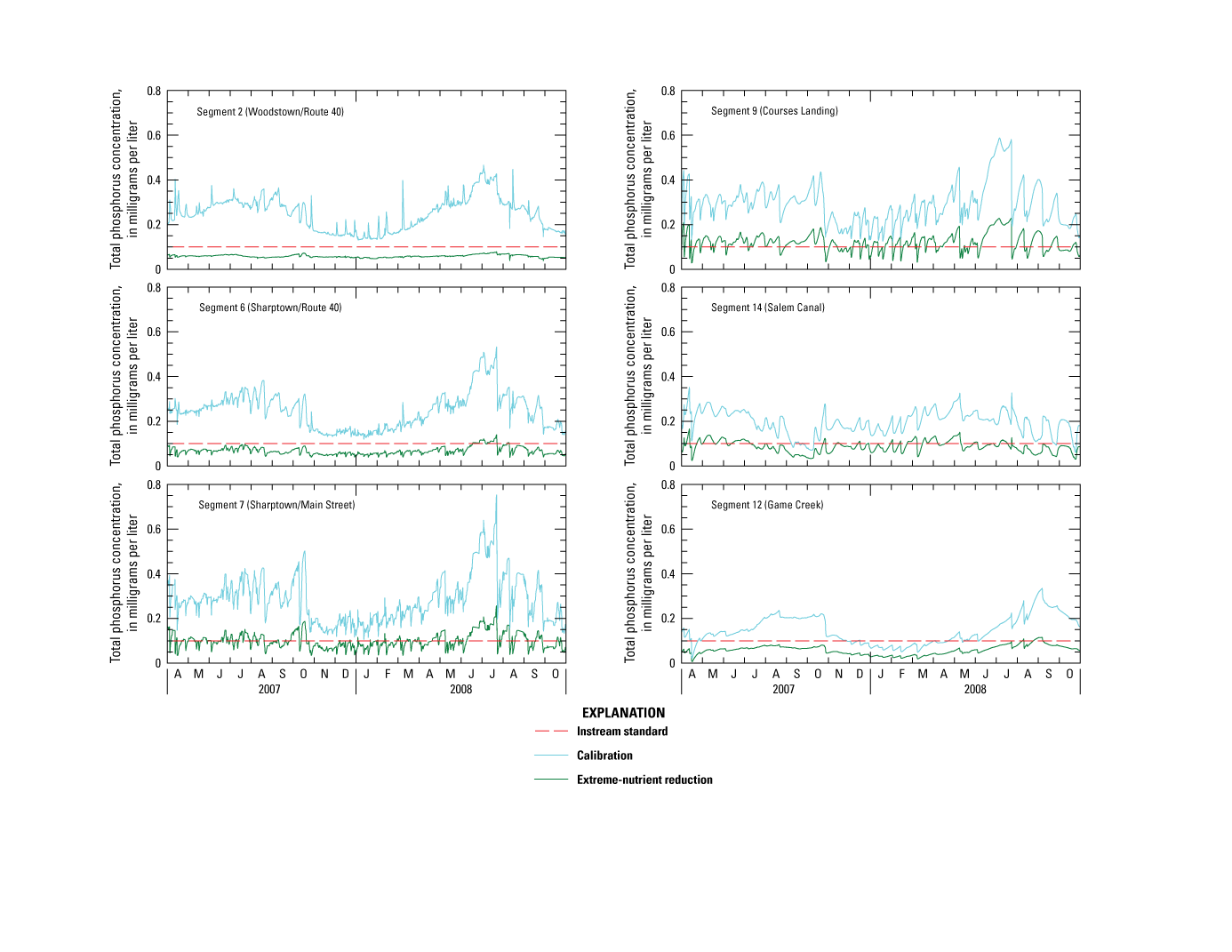
Graphs showing simulated concentration of total phosphorus for calibration and extreme-nutrient-reduction scenario, central Salem River, New Jersey, 2007–08.
Phytoplankton Chlorophyll-a
Simulated results for CHL-a for calibrated conditions and the extreme-nutrient-reduction scenario are listed in table 12 and shown in figure 31. CHL-a concentrations generally exceeded the 24-μg/L threshold during much of the growing season under calibration conditions, as discussed previously, whereas the threshold was met during the nongrowing season. Under the extreme-nutrient-reduction scenario, average CHL-a concentrations decreased 50 to 82 percent during the growing season, and the threshold was always met in riverine segments (2, 6, 7). The threshold was exceeded by as much as 20 μg/L in lacustrine segments 12 and 14 during the growing season, and by as much as 50 μg/L in segment 9.
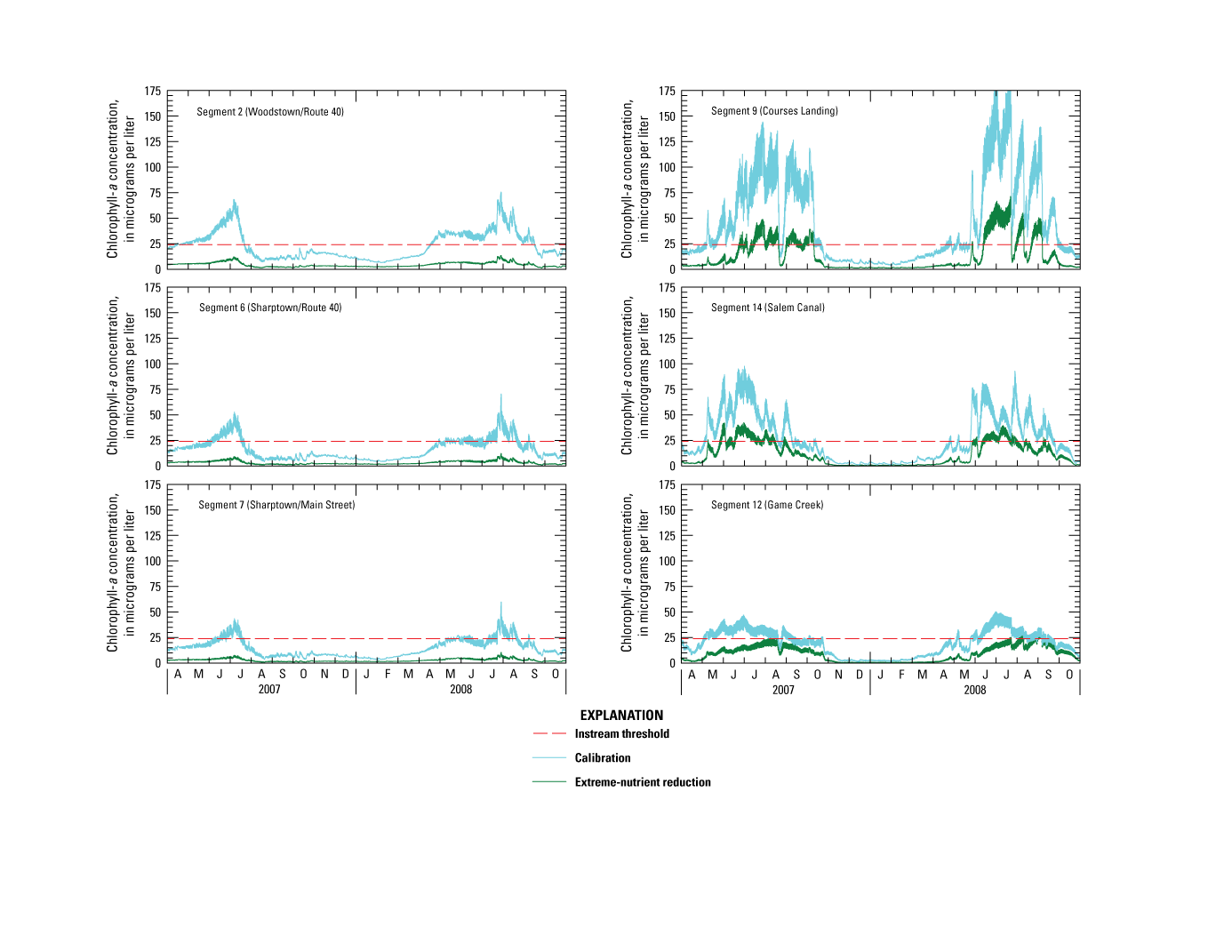
Graphs showing simulated concentration of chlorophyll-a for calibration and extreme-nutrient-reduction scenario, central Salem River, New Jersey, 2007–08.
Dissolved Oxygen
Simulated results for DO for calibrated conditions and the extreme-nutrient-reduction scenario are listed in table 12 and shown in figure 32. Only in segment 14 and intermittently in segments 9 and 12 were DO concentrations less than the minimum surface-water-quality standard of 4.0 mg/L during the growing season under calibration conditions, as discussed previously. The daily average DO concentration often exceeded the standard of 5.0 mg/L in all segments during the growing season under calibration conditions. The maximum daily variation in DO concentration was greater than the 3-mg/L guidance level in segments 9 and 14 during the growing season under calibration conditions.
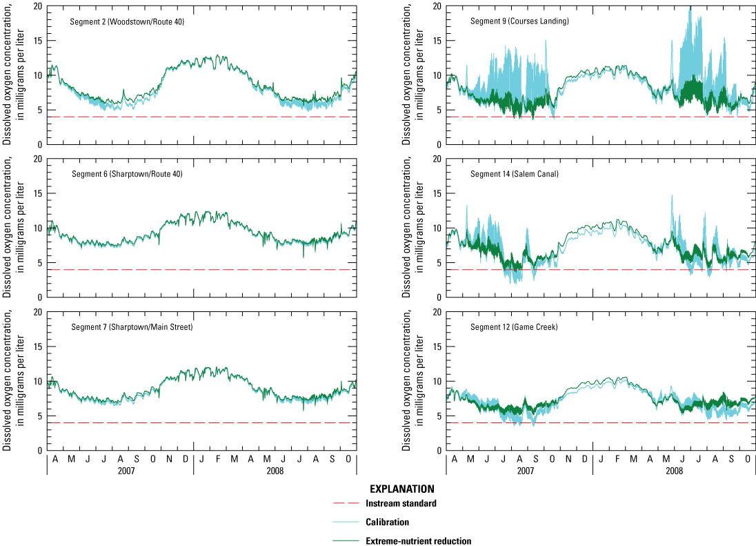
Graphs showing simulated concentration of dissolved oxygen for calibration and extreme-nutrient-reduction scenario, central Salem River, New Jersey, 2007–08.
Under the extreme-nutrient-reduction scenario, DO concentrations always exceeded the minimum 4.0-mg/L standard in segments 2, 6, 7 and 12, but not in segments 9 and 14, and were as much as 87 percent higher than under calibration conditions during the growing season. The minimum concentration standard was violated intermittently during July–September 2008 in bottom segment 16 (not shown). The daily average DO concentration exceeded the standard of 5.0 mg/L most of the time in all segments during the growing season. The maximum daily variation in DO concentration decreased by as much as 72 percent and was less than the 3-mg/L guidance level in all segments except segments 9 and 14 during the growing season. Desired outcomes of higher minimum concentrations and reduced daily range were achieved in this scenario, although an unintended consequence was lower daily average DO concentrations in segment 9 caused by reduced photosynthetic production by phytoplankton.
An assumption of the scenario design is that algal growth will be suppressed with less phosphorus in the water column, and that in turn will reduce consumption of DO. However, phosphorus and carbon accumulated in riverbed sediment can create a persistent oxygen demand by means of sediment diagenesis; that is, decomposition of organic material and mineralization of organic phosphorus and organic carbon below the riverbed-water column interface consume oxygen by means of CBOD and SOD. Long-term accumulation of organic materials in the riverbed coupled with the warm water temperatures and low flows that characterize the growing season can be responsible for low DO concentrations; under these conditions, inorganic phosphorus created through mineralization can be released back to the water column as food for algae.
Nitrogen
Simulated results for TN for calibrated conditions and the extreme-nutrient-reduction scenario are shown figure 33. Comparisons are not included in table 12 because the reduction in nitrogen in the scenario design is small. Under the extreme-nutrient-reduction scenario, TN concentrations were changed slightly in all segments compared to calibration conditions.
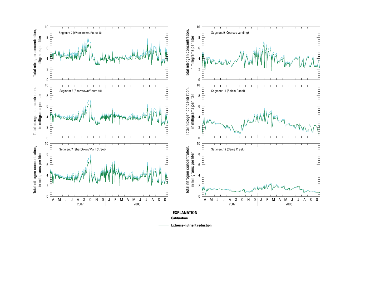
Graphs showing simulated concentration of total nitrogen for calibration and extreme-nutrient-reduction scenario, central Salem River, New Jersey, 2007–08.
Similar results were seen for NO3 and NH4 (not shown) in riverine segments. In lacustrine segments, NO3 concentrations increased during the growing season, possibly as a result of decreased algal productivity and the associated decrease in NO3 assimilation during photosynthesis. Diurnal variation in NH4 in these segments were reduced, indicating reduced photosynthesis resulting from a reduction in phytoplankton. The surface-water-quality standard for NO3 of 10 mg/L was not exceeded under calibration conditions or in the extreme-nutrient-reduction scenario.
Summary and Conclusions
Eutrophication, as indicated by excessive algal growth, occurs during the growing season in the central Salem River in New Jersey. Elevated nutrient loads that stimulate primary productivity of phytoplankton and macrophytes lead to low dissolved-oxygen (DO) concentrations, large diurnal variations in DO, and diminished water clarity, which can impair the health of aquatic life. Eutrophication in the central Salem River results from wash-off of nutrient loads from extensive application of agricultural fertilizers, agricultural animal waste, and point sources, such as wastewater effluent. As a result, the New Jersey Department of Environmental Protection (NJDEP) has mandated development of a total maximum daily load (TMDL), potentially for phosphorus, for the Salem River. Because eutrophication is a complex process, a surface-water-quality model was developed by the U.S. Geological Survey (USGS) to assist NJDEP in quantifying the effects of nutrient loads on the quality of water in the river and testing management strategies that could bring the river into compliance with applicable surface-water-quality standards.
Central Salem River is composed of upstream riverine reaches and downstream lacustrine reaches, a result of damming in the Salem Canal. Lacustrine reaches are particularly prone to the effects of eutrophication during the growing season as a result of long residence times, adjacent agriculture, and greater exposure to sunlight due to lack of tree canopy. As part of a related field study, the USGS collected water-quality samples in the river 15 times, primarily at medium to low flow during the growing season from April 2007 to October 2008. Supplemental field data were obtained through intensive sampling over a 2-month period in late summer 2008.
The U.S. Environmental Protection Agency Water-Quality Analysis Simulation Program (WASP) model was used to simulate receiving-water quality in the central Salem River. WASP includes separate modules for simulating advection that drives constituent transport and mixing, and biochemical processes controlling transformation/kinetics and other factors that affect eutrophication. The model domain included the main-stem river between Woodstown and the Salem Canal and the largest tributary (Game Creek). Effects from the upper Salem River Basin were accounted for by the upstream model boundary, and the lower Salem River was excluded from the model as a result of downstream damming. The simulation period coincided with the sampling period.
Boundary conditions for the flow model consisted of the Woodstown gage, estimated flows for tributaries along the main stem, and reported flows for the Woodstown Wastewater Treatment Plant (WWTP) and the Salem Canal diversion. Model input also included channel characteristics data to simulate kinematic wave flow in upstream reaches and ponded weir flow in downstream reaches. The water-quality model was based on a mass-balance equation to simulate DO concentrations and oxygen demands (carbonaceous biochemical oxygen demand, sediment oxygen demand), and concentrations of nitrogen species (ammonia, nitrate, dissolved organic nitrogen), phosphorus species (dissolved inorganic phosphorus, dissolved organic phosphorus), and phytoplankton chlorophyll-a (CHL-a). Upstream boundary concentrations at Woodstown were estimated from 2007–08 and historical observed data. Boundary conditions along the main stem consisted of constituent loads from tributary watersheds estimated by using regression and export coefficient methods. Because data were insufficient, storm-event sampling from areas outside the basin was used to develop load estimates. Other water-quality-model inputs included reported data on meteorological parameters and kinetic constants, and estimated vertical mixing coefficients, settling rates, and benthic fluxes.
Model calibration focused on predicting flow variables and water-quality concentrations at six locations (three riverine, two lacustrine, one tributary) with emphasis on the growing season. Simulated results and observed data were compared graphically and statistically to assess model accuracy, although statistics were of limited use as a result of the limited data. Flow was calibrated by adjusting selected model inputs until simulated streamflow, depth, velocity, and time of travel closely matched observed data. Water quality was calibrated by adjusting kinetic constants and estimated boundary conditions until simulated concentrations closely matched observed data. Simulated values generally closely matched observed data, although simulated values were slightly overpredicted in some cases. The primary cause for overprediction was estimated tributary watershed flows for the flow model and estimated tributary watershed loads for the water-quality model. Calibration of DO concentrations was good, and predicted large diurnal variations were consistent with times of high algal photosynthesis/respiration, although a lack of continuous DO data precluded verifying these predictions. A similar caveat applies to predicted diurnal variations in CHL-a. Simulated limitations on algal growth were consistent with those based on observed data and indicated phosphorus was the main limiting nutrient, except during certain periods when nitrogen was limiting.
Two model sensitivity analyses were performed: pre-calibration to identify the most sensitive model parameters and post-calibration to determine which parameters had the greatest effect on simulated constituent concentrations. Limitations associated with the data and model and the applicability of the model for TDML development were evaluated. Two water-quality management scenarios were run to evaluate the effects of nutrient-reduction strategies on eutrophication in the river: (1) return to predevelopment natural conditions and (2) extreme nutrient reduction. Both scenarios were designed by changing upstream boundary concentrations, watershed loads, WWTP loads, and oxygen demands. Simulated concentrations of total phosphorus, CHL-a, DO, and total nitrogen were compared to calibrated concentrations at six locations for each scenario. Although the extreme-nutrient-reduction scenario yielded improvements in water quality, the natural-conditions scenario yielded the largest improvements as indicated by minimal violations of surface-water-quality standards or thresholds. However, years may be needed to attain the full benefit of conditions simulated in these scenarios as a result of accumulation of phosphorus and organic carbon in riverbed sediments of lacustrine reaches—that is, water-quality improvements will be delayed until the magnitude of these sources is reduced. Also, short-term management strategies, such as decreasing residence time by means of flow releases through dam gates, tertiary treatment of phosphorus at the Woodstown WWTP, or channel dredging may not alleviate eutrophication, as some phosphorus originates in groundwater base flow from infiltration from agricultural land as well as release from sediment-bound sources, which discharge slowly to the river.
The results of this study indicate that the quality of water in the central Salem River will improve if management policies that mitigate the effects of nutrient-loading practices in the watershed, particularly those related to agriculture, are implemented. Also, other types of data collection (for example, information on algal species, benthic fluxes, water quality during high-flow conditions, continuous monitoring, intensive water-column sampling), development of a more robust flow model, and (or) development of a watershed model could improve the water-quality model and consequently allow for a more accurate representation of water-quality conditions in the river.
References Cited
Baker, R.J., and Esralew, R.A., 2010, Relation of water quality to land use in the drainage basins of six tributaries to the Lower Delaware River, New Jersey, 2002–07: U.S. Geological Survey Scientific Investigations Report2010–5151, 52 p. [Also available at https://doi.org/10.3133/sir20105151.]
Baker, R.J., and Hunchak-Kariouk, K., 2006, Relations of water quality to streamflow, season, and land use for four tributaries to the Toms River, Ocean County, New Jersey, 1994–99: U.S. Geological Survey Scientific Investigations Report2005–5274, 72 p. [Also available at https://doi.org/10.3133/sir20055274.]
Bowie, G.L., Mills, W.B., Porcella, D.B., Campbell, C.L., Pagenkopf, J.R., Rupp, G.L., Johnson, K.M., Chan, P.W.H., Gherini, S.A., and Chamberlin, C.E., 1985, Rates, constants, and kinetics formulations in surface water quality modeling, (2d ed.), EPA/600/3-85/040: Washington, D.C., U.S. Environmental Protection Agency, 455 p. [Also available at https://cfpub.epa.gov/si/si_public_record_Report.cfm?Lab=ORD&dirEntryID=34685.]
Chapra, S.C., and Canale, R.P., 1991, Long-term phenomenological model of phosphorus and oxygen for stratified lakes: Water Research, v. 25, no. 6, p. 707–715. [Also available at https://doi.org/10.1016/0043-1354(91)90046-S.]
Clesceri, N.L., Curran, S.J., and Sedlak, R.I., 1986, Nutrient loads to Wisconsin lakes—Part 1: Journal of the American Water Resources Association, v. 22, no. 6, p. 983–990. [Also available at https://doi.org/10.1111/j.1752-1688.1986.tb00769.x.]
Coon, W.F., 1998, Estimation of roughness coefficients for natural stream channels with vegetated banks: U.S. Geological Survey Water-Supply Paper2441, 133 p. [Also available at https://pubs.er.usgs.gov/publication/wsp2441.]
Covar, A.P., 1976, Selecting the proper reaeration coefficient for use in water quality models, in Ott, W.R., Proceedings of the Conference on Environmental Modeling and Simulation, Cincinnati, Ohio, April 19–22, 1976, [Proceedings]: Washington, D.C., U.S. Environmental Protection Agency, p. 340–343. [Also available at https://books.google.com/books?id=J0Jpe6q1GlcC&printsec=frontcover&source=gbs_ge_summary_r&cad=0#v=onepage&q&f=false.]
Dar, A.D., Pandit, A.K., and Ganai, B.A., 2014, Factors affecting the distribution patterns of aquatic macrophytes: Limnological Review, v. 14, no. 2, p. 75–81. [Also available at https://doi.org/10.2478/limre-2014-0008.]
DePaul, V.T., and Spitz, F.J., 2023, WASP model used to simulate flow and eutrophication in the central Salem River, New Jersey: U.S. Geological Survey data release, https://doi.org/10.5066/F78G8JPJ.
DePaul, V.T., and Szabo, Z., 2007, Occurrence of radium-224, radium-226, and radium-228 in water from the Vincentown and Wenonah-Mount Laurel aquifers, the Englishtown aquifer system, and the Hornerstown and Red Bank Sands, southwestern and south-central New Jersey: U.S. Geological Survey Scientific Investigations Report2007–5064, 62 p. [Also available at https://doi.org/10.3133/sir20075064.]
DiToro, D.M., O’Connor, D.J., and Thomann, R.V., 1971, A dynamic model of the phytoplankton population in the Sacramento—San Joaquin Delta, chap. 5 of Hem, J.D., Nonequilibrium systems in natural water chemistry: Washington, D.C., American Chemical Society, p. 131–180. [Also available at https://pubs.acs.org/doi/10.1021/ba-1971-0106.ch005.]
Engel, B., Storm, D., White, M., Arnold, J., and Arabi, M., 2007, A hydrologic/water quality model application protocol: Journal of the American Water Resources Association, v. 43, no. 5, p. 1223–1236. [Also available at https://doi.org/10.1111/j.1752-1688.2007.00105.x.]
Ernst, M.R., and Owens, J., 2009, Development and application of a water quality analysis simulation program model on a large Texas reservoir to assess eutrophication control: Lake and Reservoir Management, v. 25, no. 2, p. 136–148. [Also available at https://doi.org/10.1080/07438140902821389.]
Fitzpatrick, J.J., 2009, Assessing skill of estuarine and coastal eutrophication models for water quality managers: Journal of Marine Systems, v. 76, no. 1–2, p. 195–211. [Also available at https://doi.org/10.1016/j.jmarsys.2008.05.018.]
Hammerschmidt, C.R., and Mullen, K.R., 2016, Benthic phosphorus fluxes in the Lower Great Miami River: Miami Conservancy District Report No. 2016–10, 26 p. [Also available at https://www.mcdwater.org/wp-content/uploads/2017/08/Benthic-Phosphorus-Fluxes.pdf.]
Heckathorn, H.A., and Gibs, J., 2010, Sediment oxygen demand in the Saddle River and Salem River watersheds, New Jersey, July–August 2008: U.S. Geological Survey Scientific Investigations Report2010–5093, 10 p. [Also available at https://doi.org/10.3133/sir20105093.]
Hunchak-Kariouk, K., Buxton, D.E., and Hickman, R.E., 1999, Relations of surface-water quality to streamflow in the Atlantic Coastal, Lower Delaware River, and Delaware Bay Basins, New Jersey, water years 1976–93: U.S. Geological Survey Water-Resources Investigations Report 98–4244, 146 p. [Also available at https://doi.org/10.3133/wri984244.]
Kuwabara, J.S., Topping, B.R., Lynch, D.D., Carter, J.L., and Essaid, H.I., 2009, Benthic nutrient sources to hypereutrophic Upper Klamath Lake, Oregon, USA: Environmental Toxicology and Chemistry, v. 28, no. 3, p. 516–524. [Also available at https://doi.org/10.1897/08-207.1.]
Legates, D.R., and McCabe, G.J., 1999, Evaluating the use of “goodness-of-fit” measures in hydrologic and hydroclimatic model validation: Water Resources Research, v. 35, no. 1, p. 233–241. [Also available at https://doi.org/10.1029/1998WR900018.]
Litke, D.W., 1999, Review of phosphorus control measures in the United States and their effects on water quality: U.S. Geological Survey Water-Resources Investigations Report99–4007, 38 p. [Also available at https://doi.org/10.3133/wri994007.]
McFarland, A.M.S., and Hauck, L.M., 2001, Determining nutrient export coefficients and source loading uncertainty using in-stream monitoring data: Journal of the American Water Resources Association, v. 37, no. 1, p. 223–236. [Also available at https://doi.org/10.1111/j.1752-1688.2001.tb05488.x.]
Moriasi, D.N., Gitau, M.W., Pai, N., and Daggupati, P., 2015, Hydrologic and water quality models—Performance measures and evaluation criteria: Transactions of the ASABE, v. 58, no. 6, p. 1763–1785. [Also available at https://doi.org/10.13031/trans.58.10715.]
Munn, M.D., Frey, J.W., Tesoriero, A.J., Black, R.W., Duff, J.H., Lee, K., Maret, T.R., Mebane, C.A., Waite, I.R., and Zelt, R.B., 2018, Understanding the influence of nutrients on stream ecosystems in agricultural landscapes: U.S. Geological Survey Circular 1437, 80 p. [Also available at https://doi.org/10.3133/cir1437.]
New Jersey Department of Environmental Protection, 2003a, Total maximum daily loads for phosphorus to address 13 eutrophic lakes in the Lower Delaware Water Region [Amendment to the Atlantic County Water Quality Management Plan, Lower Delaware Water Quality Management Plan, Mercer County Water Quality Management Plan, Monmouth County Water Quality Management Plan, Tri-County Water Quality Management Plan]: Trenton, N.J., New Jersey Department of Environmental Protection, Division of Watershed Management, 76 p. [Also available at https://www.nj.gov/dep/wms/bears/docs/Lower%20Delaware%20Lakes.pdf.]
New Jersey Department of Environmental Protection, 2003b, New Jersey 2002 Integrated Water Quality Monitoring and Assessment Report, New Jersey Department of Environmental Protection Water Assessment Team, accessed November 20, 2008, at https://www.nj.gov/dep/gis/digidownload/metadata/ir/ir_river_all.htm.
New Jersey Department of Environmental Protection, 2007, NJDEP 2002 land use/land cover update, Maurice, Salem, and Cohansey Watershed Management Area, WMA–17, Edition 20080304: New Jersey Department of Environmental Protection, accessed February 1, 2009, at https://www.state.nj.us/dep/gis/digidownload/metadata/lulc02/w17lu02.htm.
New Jersey Department of Environmental Protection, 2009a, 2008 New Jersey integrated water quality monitoring and assessment report: New Jersey Department of Environmental Protection, Division of Water Monitoring and Standards, 403 p. [Also available at https://www.state.nj.us/dep/wms/bears/docs/2008_final_IR_complete.pdf.]
New Jersey Department of Environmental Protection, 2009b, Department of Environmental Protection DataMiner: New Jersey Department of Environmental Protection, accessed July 1, 2009, at https://njems.nj.gov/DataMiner/Search/SearchByCategory?isExternal=y&getCategory=y&catName=NJPDES%20Permitting%20Program.
New Jersey Department of Environmental Protection, 2010, Ambient biomonitoring network: New Jersey Department of Environmental Protection, Division of Water Monitoring and Standards, 233 p. [Also available at https://www.nj.gov/dep/wms/bfbm/download/ldlRnd3.pdf.]
New Jersey Department of Labor and Workforce Development, 2021, Population, Housing Units, and Density 2020 Census—Census 2020 Redistricting File—New Jersey State and Counties: New Jersey Department of Labor and Workforce Development, accessed December 1, 2022, at https://www.nj.gov/labor/labormarketinformation/assets/PDFs/census/2020/2020%20pl94%20Tables/2020_PL94_Summary/densityCTY_2020.xlsx.
Omni Environmental, 2007, The non-tidal Passaic River Basin nutrient total maximum daily load study—Phase II Watershed model and TMDL calculations: Princeton, N.J., Omni Environmental, 189 p. [Also available at https://www.nj.gov/dep/wms/bears/docs/passaic_final_report20070223.pdf.]
Redfield, A.C., 1958, The biological control of chemical factors in the environment: American Scientist, v. 46, no. 3, p. 205–221. [Also available at https://www.jstor.org/stable/pdf/27827150.]
Runkel, R.L., Crawford, C.G., and Cohn, T.A., 2004, Load estimator (LOADEST)—A FORTRAN program for estimating constituent loads in streams and rivers: U.S. Geological Survey Techniques and Methods, book 4, chap. A5, 69 p. [Also available at https://doi.org/10.3133/tm4A5.]
Rutgers Cooperative Extension Water Resources Program, 2012, Upper Salem River watershed restoration and protection plan: Water Resources Program, Rutgers University, 103 p., 2 app. [Also available at https://water.rutgers.edu/Projects/UpperSalem/FINAL_Salem_Restoration_Plan_Complete.pdf.]
Sauer, V.B., 2002, Standards for the analysis and processing of surface-water data and information using electronic methods: U.S. Geological Survey Water-Resources Investigations Report01–4044, 91 p. [Also available at https://doi.org/10.3133/wri20014044.]
Shoemaker, L., Lahlou, M., Bryer, M., Kumar, D., and Kratt, K., 1997, Compendium of tools for watershed assessment and total maximum daily load development: U.S. Environmental Protection Agency, Office of Water, 244 p. [Also available at https://nepis.epa.gov/Exe/ZyPDF.cgi/20004NX4.PDF?Dockey=20004NX4.PDF.]
Smith, R.A., 1980, The theoretical basis for estimating phytoplankton production and specific growth rate from chlorophyll, light and temperature data: Ecological Modelling, v. 10, no. 3–4, p. 243–264. [Also available at https://doi.org/10.1016/0304-3800(80)90062-9.]
Smith, R.A., Alexander, R.B., and Schwarz, G.E., 2003, Natural background concentrations of nutrients in streams and rivers of the conterminous United States: Environmental Science & Technology, v. 37, no. 14, p. 3039–3047. [Also available at https://doi.org/10.1021/es020663b.]
State of New Jersey, 2008, Technical manual for phosphorus evaluations–—NJPDES discharge to surface water permits: New Jersey Department of Environmental Protection, 62 p. [Also available at https://www.nj.gov/dep/dwq/pdf/p-manual-07-30-08.pdf.]
State of New Jersey, 2020, Surface water quality standards: New Jersey Department of Environmental Protection, 113 p. [Also available at https://www.nj.gov/dep/rules/rules/njac7_9b.pdf.]
Sugarman, P.J., 1999, Radon potential of New Jersey Coastal Plain formations: New Jersey Geological Survey Open-File Map 25, 1 pl., scale 1:250,000. [Also available at https://www.state.nj.us/dep/njgs/pricelst/ofmap/ofm25.pdf.]
Sullivan, A.B., Rounds, S.A., Uhrich, M.A., and Bragg, H.M., 2006, Modeling suspended sediment and water temperature in Detroit Lake, Oregon, in Proceedings of the Eighth Federal Interagency Sedimentation Conference, Reno, Nev., April 2–6, 2006, [Proceedings]: Advisory Committee on Water Information, p. 745–750. [Also available at https://pubs.usgs.gov/misc/FISC_1947-2006/pdf/1st-7thFISCs-CD/8thFISC/Session%2010A-4_Sullivan.pdf.]
U.S. Department of Agriculture, 2008, Soil survey of Salem County, New Jersey—U.S.: Washington, D.C., U.S. Department of Agriculture, 375 p. [https://www.nrcs.usda.gov/Internet/FSE_MANUSCRIPTS/new_jersey/NJ033/0/NJSalem06_08.pdf.]
U.S. Department of Agriculture, 2012, County summary highlights—2012, table 1 of 2012 Census of Agriculture County data: U.S. Department of Agriculture, Census of Agriculture Historical Archive, accessed February 15, 2022, at https://agcensus.library.cornell.edu/wp-content/uploads/2012-New_Jersey-st34_2_001_001.pdf.
U.S. Environmental Protection Agency, 1995, Technical guidance manual for developing total maximum daily loads, EPA–823–B–95–007: Washington, D.C., U.S. Environmental Protection Agency, Office of Water, 254 p. [Also available at https://nepis.epa.gov/Exe/ZyPURL.cgi?Dockey=200055WG.txt.]
U.S. Environmental Protection Agency, 2001, PLOAD version 3.0—An ArcView GIS tool to calculate nonpoint sources of pollution in watershed and stormwater projects [User’s manual]: Washington, D.C., U.S. Environmental Protection Agency, Office of Water, 44 p. [Also available at https://permanent.fdlp.gov/lps49376/PLOAD_v3.pdf.]
U.S. Environmental Protection Agency, 2007a, Advanced wastewater treatment to achieve low concentration of phosphorus: Seattle, Wash., U.S. Environmental Protection Agency, Office of Water and Watersheds, 73 p. [Also available at https://www.epa.gov/sites/default/files/2019-02/documents/advanced-wastewater-treatment-low-concentration-phosphorus.pdf.]
U.S. Environmental Protection Agency, 2007b, Options for expressing daily loads in total maximum daily loads: Washington, D.C., U.S. Environmental Protection Agency, Office of Wetlands, Oceans, and Watersheds, 50 p. [Also available at https://www.epa.gov/sites/default/files/2015-07/documents/2007_06_26_tmdl_draft_daily_loads_tech.pdf.]
U.S. Environmental Protection Agency, 2007c, An approach for using load-duration curves in the development of total maximum daily loads: Washington, D.C., U.S. Environmental Protection Agency, Office of Wetlands, Oceans, and Watersheds, 68 p. [Also available at https://www.epa.gov/sites/default/files/2015-07/documents/2007_08_23_tmdl_duration_curve_guide_aug2007.pdf.]
U.S. Geological Survey, 2022, USGS water data for the Nation: U.S. Geological Survey National Water Information System database, accessed April 1, 2022, at https://waterdata.usgs.gov/nwis/.
University of Delaware, 2009, Historical monthly station summary retrieval: Delaware Environmental Observing System, University of Delaware, accessed July 1, 2009, at http://www.deos.udel.edu/data/monthly_retrieval.php.
Weiss, R.F., 1970, The solubility of nitrogen, oxygen and argon in water and seawater: Deep-Sea Research, v. 17, no. 4, p. 721–735. [Also available at https://www.sciencedirect.com/science/article/pii/0011747170900379.]
Wood, T., and Rounds, S., 1998, Using CE-QUAL-W2 to assess the effect of reduced phosphorus loads on chlorophyll-a and dissolved oxygen in the Tualatin River, Oregon, in Proceedings of the First Federal Interagency Hydrologic Modeling Conference, Las Vegas, Nev., April 19–23, 1998, [Proceedings]: Advisory Committee on Water Information, v. 2, p. 149–156. [Also available at https://or.water.usgs.gov/tualatin/phos_tual_fihmc.pdf.]
Wool, T.A., Ambrose, R.B., Martin, J.L., and Comer, E.A., 2003, Water quality analysis simulation program—Version 6.0 draft user’s manual: U.S. Environmental Protection Agency, Region 4, Atlanta, Ga., 267 p. [Also available at https://www.researchgate.net/publication/26991027_Water_Quality_Analysis_Simulation_Program_WASP.]
Wurtsbaugh, W.A., Paerl, H.W., and Dodds, W.K., 2019, Nutrients, eutrophication and harmful algal blooms along the freshwater to marine continuum: WIREs Water, v. 6, no. 5, 27 p. [Also available at https://doi.org/10.1002/wat2.1373.]
YSI Inc., 2021, Phosphorus in wastewater: Yellow Springs, Ohio, YSI Inc., 43 p. [Also available at https://www.ysi.com/phosphorus-in-wastewater.]
Zhang, W., and Rao, Y.R., 2012, Application of a eutrophication model for assessing water quality in Lake Winnipeg: Journal of Great Lakes Research, v. 38, sup. 3, p. 158–173. [Also available at https://www.sciencedirect.com/science/article/pii/S0380133011000050.]
Conversion Factors
International System of Units to U.S. customary units
Temperature in degrees Celsius (°C) may be converted to degrees Fahrenheit (°F) as °F = (1.8 × °C) + 32.
Temperature in degrees Fahrenheit (°F) may be converted to degrees Celsius (°C) as °C = (°F – 32) / 1.8.
Datum
Vertical coordinate information is referenced to the North American Vertical Datum of 1988 (NAVD 88).
Horizontal coordinate information is referenced to North American Datum of 1983 (NAD 83).
Altitude, as used in this report, refers to distance above the vertical datum.
Supplemental Information
Concentrations of chemical constituents in water are given in milligrams per liter (mg/L) or micrograms per liter (µg/L).
Abbreviations
C
carbon
CBOD
carbonaceous biochemical oxygen demand
CBODu
ultimate carbonaceous biochemical oxygen demand
CHL-a
phytoplankton chlorophyll-a
DIN
dissolved inorganic nitrogen
DIP
dissolved inorganic phosphorus
DO
dissolved oxygen
DOC
dissolved organic carbon
DON
dissolved organic nitrogen
DOP
dissolved organic phosphorus
EPA
U.S. Environmental Protection Agency
LOADEST
Load Estimator Program
N
nitrogen
NBOD
nitrogenous biochemical oxygen demand
NH4
ammonia
NJDEP
New Jersey Department of Environmental Protection
NO2
nitrite
NO3
nitrate
P
phosphorus
PLOAD
GIS pollutant loading application
PN
particulate nitrogen
PON
particulate organic nitrogen
POP
particulate organic phosphorus
PP
particulate phosphorus
SOD
sediment oxygen demand
TC
total carbon
TMDL
total maximum daily load
TN
total nitrogen
TOC
total organic carbon
TP
total phosphorus
TSS
total suspended solids
USGS
U.S. Geological Survey
WASP
Water Quality Analysis Simulation Program
WWTP
wastewater-treatment plant
≤
less than or equal to
For additional information, contact:
Director, New Jersey Water Science Center
U.S. Geological Survey
3450 Princeton Pike
Suite 110
Lawrenceville, NJ 08648
Or visit our website at:
https://www.usgs.gov/centers/new-jersey-water-science-center
Publishing support provided by the West Trenton Publishing Service Center
Suggested Citation
Spitz, F.J., and DePaul, V.T., 2023, Simulation of flow and eutrophication in the central Salem River, New Jersey: U.S. Geological Survey Scientific Investigations Report 2022–5047, 72 p., https://doi.org/10.3133/sir20225047.
ISSN: 2328-0328 (online)
Study Area
| Publication type | Report |
|---|---|
| Publication Subtype | USGS Numbered Series |
| Title | Simulation of flow and eutrophication in the central Salem River, New Jersey |
| Series title | Scientific Investigations Report |
| Series number | 2022-5047 |
| DOI | 10.3133/sir20225047 |
| Year Published | 2023 |
| Language | English |
| Publisher | U.S. Geological Survey |
| Publisher location | Reston, VA |
| Contributing office(s) | New Jersey Water Science Center |
| Description | Report: x, 72 p.; Data Release |
| Country | United States |
| State | New Jersey |
| Other Geospatial | Central Salem River |
| Online Only (Y/N) | Y |
| Additional Online Files (Y/N) | N |
| Google Analytic Metrics | Metrics page |