

Comparison of Surrogate Models To Estimate Pesticide Concentrations at Six U.S. Geological Survey National Water Quality Network Sites During Water Years 2013–18
Links
- Document: Report (12.9 MB pdf) , HTML , XML
- Data Release: USGS data release - Datasets for comparison of surrogate models to estimate pesticide concentrations at six U.S. Geological Survey National Water Quality Network sites during water years 2013–2018
- Download citation as: RIS | Dublin Core
Abstract
During water years 2013–18, the U.S. Geological Survey National Water-Quality Assessment Project sampled the National Water Quality Network for Rivers and Streams year-round and reported on 221 pesticides at 72 sites across the United States. Pesticides are difficult to measure, their concentrations often represent discrete snapshots in time, and capturing peak concentrations is expensive. Three types of regression models were developed to estimate concentrations for two selected pesticides at each of six National Water Quality Network for Rivers and Streams sites. The regression models used continuously measured streamflow and water-quality properties (differing combinations of pH, specific conductance, turbidity, and water temperature); discrete water-quality samples analyzed for atrazine, azoxystrobin, bentazon, bromacil, imidacloprid, simazine, and triclopyr; and time as an additional explanatory variable for seasonality.
The modeling approaches included (1) a standard regression that included surrogates (differing combinations of pH, specific conductance, turbidity, and water temperature) and periodic functions (sine-cosine) of pesticide application use as predictor variables; (2) the seasonal wave with flow adjustment model that included a seasonal component and flow anomalies but excluded surrogates; and (3) the seasonal wave with flow adjustment model that included a seasonal component, flow anomalies, and surrogates. Models were evaluated using three measures of model performance: generalized coefficient of determination (generalized R2), Akaike’s Information Criteria, and scale (the estimated standard deviation of the tobit regression error term). Because of low observation numbers, results from this study can be considered a pilot effort with the possibility that some models are overfit.
In all cases, estimated pesticide concentrations modeled with base SEAWAVE-Q were better than the standard surrogate regression models; all 39 generalized R2 values increased by 3–56 percent (median of 25 percent) when compared to the standard surrogate regression models, and all Akaike’s Information Criteria and scale values decreased. The addition of surrogate variables such as pH, specific conductance, turbidity, and water temperature to the base SEAWAVE-Q model to improve estimates of pesticide concentrations resulted in only modest improvements; generalized R2 values increased by only 0–10 percent (median of 3 percent). In some instances, combinations of the surrogates produced more appreciative improvements in model results, but in those instances, we hypothesize that the surrogates correlated with some unknown measure that directly relates to pesticide transport.
Introduction
In the United States, more than half a billion pounds (more than 226,700,000 kilograms) of pesticides were used annually from 2013 to 2017, including the use of more than 400 different pesticides during any given year, to maintain and improve crop production by controlling weeds, insects, and other pests (Wieben, 2019). Pesticides can enter rivers and streams through transport mechanisms such as shallow groundwater transport and runoff from precipitation and irrigation. Despite the many benefits that pesticides provide, they can potentially harm human and ecological health (Covert and others, 2020; Miller and others, 2020, Norman and others, 2020; Alvarez and others, 2021; Amenyogbe and others, 2021; Bradley and others, 2021; Nowell and others, 2021).
During water years (WY) 2013–18, the U.S. Geological Survey (USGS) National Water-Quality Assessment Project sampled the National Water Quality Network for Rivers and Streams (hereafter, referred to as NWQN) year-round and reported on 221 pesticides at 72 sites across the United States with the goal of better understanding the Nation’s water quality, including the occurrence of pesticides in natural waters (Rowe and others, 2013). A WY begins October 1 of the previous calendar year and ends September 30 of the named water year. There are a few issues that make measuring pesticide concentrations difficult: (1) the seasonality of pesticide concentrations differs from that of most other water-quality constituents; (2) the relation between streamflow and pesticide concentrations is complex; (3) the use of gas chromatography often results in censored data (concentrations that are lower than can be reliably detected by the analytical method used); and (4) pesticide sampling frequencies are often intermittent or low (Vecchia and others, 2008).
To help address these issues, a parametric regression model, SEAWAVE-Q, was specifically developed to analyze trends in chemical concentrations in streams with a seasonal wave (SEAWAVE), an adjustment for streamflow (Q), and other ancillary variables (Vecchia and others, 2008; Ryberg and York, 2020). Because of its robustness in fitting the seasonal patterns of pesticide occurrence in streams across various regions of the United States and its ability to handle large amounts of censored concentration data, SEAWAVE-Q has been used to analyze pesticide trends in several studies (Sullivan and others, 2009; Ryberg and others, 2010; Ryberg and others, 2014; Ryberg and Gilliom, 2015; Oelsner and others, 2017). Still, two issues remain when measuring pesticide concentrations. First, discrete samples are snapshots in time and do not always represent extreme concentrations (Norman and others, 2020). These discrete samples, then, likely underrepresent potential toxicity. NWQN data collection was not intended to characterize the highest concentrations; therefore, NWQN data are likely to be underestimates of actual peak concentrations. Second, other collection methods, such as autosamplers and polar organic chemical integrative samplers, can measure these higher extremes, but the number of discrete samples needed to estimate extreme pesticide concentrations each year would be cost prohibitive for an ambient network (Crawford, 2004).
Pesticide surrogate models have the potential to address these needs by providing near-real-time estimates of pesticide concentrations. For the purposes of this investigation, a surrogate (differing combinations of pH, specific conductance, turbidity, and water temperature) is a continuous in-stream sensor measurement used to compute or estimate the concentration of a water-quality constituent of greater interest (that is, pesticide concentrations; USGS, 2021b). Surrogates also have the potential to be easier and (or) cheaper to measure; for example, turbidity is regularly used as a surrogate for measuring suspended sediment, and specific conductance is used as a surrogate for estimating chloride concentrations (Christensen and others, 2000; Ryberg, 2006; Jastram and others, 2009; Rasmussen and others, 2009; Wood and Teasdale, 2013). The SEAWAVE-Q model already includes variables that represent seasonality and streamflow but also allows for other continuously monitored properties such as pH, specific conductance, turbidity, and water temperature to be used as surrogate variables.
Purpose and Scope
This report documents the development and comparison of three types of regression models using data collected during WY 2013–18 to estimate selected pesticide concentrations at six USGS streamflow-gaging stations. The modeling approaches included (1) a regression that included surrogates and periodic functions (sine-cosine) that are commonly used to model seasonality in concentration data (hereafter referred to as standard surrogate regression); (2) the seasonal wave with flow adjustment (SEAWAVE-Q/RCS-4) model that used restricted cubic splines (RCS) with four knots and included a seasonal component and flow anomalies but excluded surrogates (hereafter referred to as base SEAWAVE-Q); and (3) the seasonal wave with flow adjustment (SEAWAVE-Q/RCS-4) model that used RCS with four knots and included a seasonal component, flow anomalies, and surrogates (hereafter referred to as SEAWAVE-Q [with surrogates]).
Continuously measured streamflow was used in the base SEAWAVE-Q and SEAWAVE-Q (with surrogates) models but not in the standard surrogate regression. Continuously measured water-quality properties (differing combinations of pH, specific conductance, turbidity, and water temperature) were used as surrogates in the standard surrogate regression and SEAWAVE-Q (with surrogates) models. All three types of regression models used discrete water-quality samples analyzed for atrazine, azoxystrobin, bentazon, bromacil, imidacloprid, simazine, or triclopyr (two pesticides per site) and functions of time as additional explanatory variables for seasonality. The purpose of this report was to determine (1) whether the addition of streamflow and seasonality as represented in the base SEAWAVE-Q model produced better fit results than the standard surrogate regression models; and (2) whether the addition of surrogates to the base SEAWAVE-Q model produced better fit results than either standard surrogate regression or base SEAWAVE-Q models.
Study Design and Methods
The NWQN was established in 2013 and consists of sites from a few historical water-quality monitoring networks such as the National Water-Quality Assessment, the National Stream Quality Accounting Network, and the National Monitoring Network with the goal of developing a long-term, consistent network to track the status and trends of the Nation's water quality (Riskin and Lee, 2021). At the time of this investigation, the network comprises about 110 sites (number of sites may vary slightly among years), including 74 river and stream sites with pesticide sampling (Lee and Reutter, 2019; USGS, 2021a).
NWQN Pesticide Sample Collection
During WY 2013–18, between 12 and 33 depth- and width-integrated water samples were collected at each NWQN river and stream site using methods described in USGS (variously dated). A total of 221 pesticides were analyzed in filtered (0.7 μm) water samples at the USGS National Water Quality Laboratory using direct-aqueous injection liquid chromatography with tandem mass spectrometry (Sandstrom and others, 2015).
Selected Sites, Pesticides, and Surrogates Used in Regression Models
Whereas the NWQN analyzed 221 pesticides at 72 sites across the United States, this investigation analyzed 12 site-pesticide combinations (two pesticides for each of six sites) that were chosen on the basis of the availability of pesticide, streamflow, and surrogate data collected from the NWQN river and stream sites (fig. 1; table 1). These six sites were among seven NWQN sites with continuous water-quality monitors. One site, the Ohio River at Olmsted, Illinois, was excluded from this study owing to concerns of how well the data from the water-quality monitor represented values in the channel cross section. Pesticides were analyzed from discrete water-quality samples and included frequently detected pesticides from several classes: atrazine, bentazon, bromacil, simazine, and triclopyr (herbicides); imidacloprid (insecticide); and azoxystrobin (fungicide). Similarly, this study also selected four continuously measured water-quality properties (differing combinations of pH, specific conductance, turbidity, and water temperature including 1-day anomaly values for each) as potential explanatory variables (in other words, surrogates; table 2) in pesticide concentration regression models on the basis of the availability of continuous data at the NWQN pesticide sites. Pesticide concentration, streamflow, and surrogate data (continuously measured field parameters) are available online from the USGS National Water Information System database (USGS, 2020) and the USGS data release associated with this report (Perkins and Bunch, 2022).
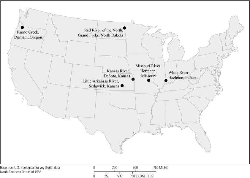
Map of six pesticide trend sites in the National Water Quality Network during water years 2013–18.
Table 1.
Site information for six sites in the National Water Quality Network during water years 2013–18.[USGS, U.S. Geological Survey; ID, identification]
Table 2.
Combinations of surrogate variables used in the standard surrogate regression and SEAWAVE-Q (with surrogates) models at six National Water Quality Network sites during water years 2013–18.[mtfa, midterm flow anomalies computed using 30 days of daily streamflow; stfa, short-term flow anomalies computed using 1 day of daily streamflow; TBY, daily median turbidity; SC, daily mean specific conductance; Temp, daily mean water temperature; pH, daily median pH; SC1d, short-term specific conductance anomalies computed using 1 day of daily specific conductance values; pH1d, short-term pH anomalies computed using 1 day of daily pH values; TBY1d, short-term turbidity anomalies computed using 1 day of daily turbidity values]
Pesticide and Surrogate Data Preparation for Regression Models
The processes for retrieving and preparing data for regression models followed those outlined in the SEAWAVE-Q R package documentation (Ryberg and Vecchia, 2013; Ryberg and York, 2020). The R package waterData (Ryberg and Vecchia, 2012) was used to import daily mean values for streamflow and either daily mean or daily median values for continuous water-quality constituents directly into R, depending on what data were available at each site. The waterData package was used to screen for missing daily mean streamflow values (no missing values were found for the sites) and to calculate short-term (1 day) and midterm (30 day) anomalies for flow and short-term anomalies (1 day) for each water-quality variable. A midterm streamflow anomaly, for instance, is the deviation of concurrent daily streamflow from average conditions for the previous 30 days (Vecchia and others, 2008). Anomalies were calculated as additional potential model variables.
Pesticide concentrations for select constituents from each site were imported to R using the dataRetrieval package (De Cicco and others, 2018). Three of the six sites (Kansas River at DeSoto, Kansas; Missouri River at Hermann, Missouri; and White River at Hazleton, Indiana) used pesticide data for WY 2013–17 whereas the other three sites (Fanno Creek at Durham, Oregon; Little Arkansas River near Sedgwick, Kansas; and Red River of the North at Grand Forks, North Dakota) used pesticide data for WY 2013–18 (table 3). Replicate samples were inadvertently included in the analysis at two sites: three samples at Little Arkansas River near Sedgwick, Kansas, and nine samples at Kansas River at DeSoto, Kansas. Discrete pesticide data were matched with daily mean streamflow and daily mean or median water-quality constituents and the associated calculated short-term (1-day) and midterm (30-day) anomalies from the date of sampling. The matched data were then used to assess selected combinations of variables in the regression models (table 2).
Table 3.
Number of observations with censored data for 12 National Water Quality Network site-pesticide combinations during water years 2013–18.[Values in parentheses are the percentage of censored values. ID, identification; FC, Fanno Creek at Durham, Oregon; -, not applicable; %, percent; *, Pesticides analyzed for water years 2013–17; HAZ, White River at Hazleton, Indiana; KR, Kansas River at DeSoto, Kansas; LAR, Little Arkansas River near Sedgwick, Kansas; MR, Missouri River at Hermann, Missouri; RR, Red River of the North at Grand Forks, North Dakota]
| Site ID (table 1) | Total number of observations | Atrazine | Azoxystrobin | Bentazon | Bromacil | Imidacloprid | Simazine | Triclopyr |
|---|---|---|---|---|---|---|---|---|
| FC | 152 | - | - | - | - | - | 24 (15.8%) | 19 (12.5%) |
| HAZ* | 89 | 0 (0) | - | - | - | 13 (14.6%) | - | - |
| KR* | 83 | 0 (0) | 2 (2.4%) | - | - | - | - | - |
| LAR | 111 | 1 (0.9%) | - | - | 5 (4.5%) | - | - | - |
| MR* | 70 | 0 (0) | 7 (10.0%) | - | - | - | - | - |
| RR | 82 | 3 (3.7%) | - | 3 (3.7%) | - | - | - | - |
Statistical Methods for Analyzing Trends in Pesticide Concentrations
Three types of regression models were developed to estimate concentrations for two selected pesticides at each of six NWQN sites.
Standard Surrogate Regression Model
The first type of regression model from Helsel and others (2020) included surrogates and periodic functions (sine-cosine) that are commonly used to model seasonality in concentration data (Ryberg and York, 2020). The model is expressed as the following:
whereY
is pesticide concentration, in micrograms per liter;
T
is decimal time, in years;
sin
is the trigonometric sine function;
cos
is the trigonometric cosine function;
π
is the mathematical constant pi;
β0, β1, …
are regression coefficients;
X1, X2, …
are explanatory variables such as pH, specific conductivity, water temperature, or turbidity; and
ε
are residuals.
The standard surrogate regression model (eq. 1) was fitted to the pesticide data using maximum likelihood methods for censored data (tobit regression). The function survreg from the R package survival, version 3.2–7 (Therneau, 2020), was used to perform the tobit regressions. Version 4.02 of R (R Core Team, 2020) was used to develop the tobit regression.
Base SEAWAVE-Q and SEAWAVE-Q (With Surrogates) Models
The second (base SEAWAVE-Q) and third (SEAWAVE-Q [with surrogates]) types of regression models in this study used the seasonal wave with flow adjustment (SEAWAVE-Q/RCS-4) model that included a seasonal component and flow anomalies (Vecchia and others, 2008; Sullivan and others, 2009; Ryberg and others, 2010, 2014; Ryberg and Vecchia, 2013). The only difference between the two models was that the base SEAWAVE-Q model did not include surrogates whereas the SEAWAVE-Q (with surrogates) model included differing combinations of pH, specific conductance, turbidity, and water temperature as explanatory variables (table 2). The original SEAWAVE-Q model assumes linear trends, but an RCS option was added that allows the time variable in SEAWAVE-Q to be split up, with “knots” defining the end of one segment and the start of the next, which is important when measuring pesticides that sometimes have nonlinear changes in usage (Ryberg and York, 2020). The development of the SEAWAVE-Q functionality for RCS models found that four knots were sufficient (Ryberg and York, 2020). All pesticide concentration estimates in this study using the base SEAWAVE-Q or SEAWAVE-Q (with surrogates) models included the RCS option using four knots and are expressed as the following:
(2)
log
denotes the base-10 logarithm;
C
is pesticide concentration, in micrograms per liter;
t
is decimal time, in years, with respect to an arbitrary time origin;
β0, β1, …
are regression coefficients;
W
is a seasonal wave representing periodic (seasonal) variability in concentration;
LTFA, MTFA, and STFA
are dimensionless long-term, midterm, and short-term streamflow anomalies computed from daily streamflow;
Sk
are cubic spline components;
k
is the number of knots; and
η(t)
is the model error.
The base SEAWAVE-Q and SEAWAVE-Q (with surrogates) models (eq. 2) were fitted to the pesticide data by maximum likelihood methods for censored data (Sullivan and others, 2009) using the statistical software R, version 4.0.3 (R Core Team, 2020), and the R extension package seawaveQ, version 2.0.2 (Ryberg and Vecchia, 2013; Ryberg and York, 2020). Surrogates were included in the SEAWAVE-Q and SEAWAVE-Q (with surrogates) models by calculating dimensionless anomalies using the waterData package, which were used as ancillary variables (Ryberg and Vecchia, 2012).
Regression Model Comparison Criteria
Continuous streamflow, pH, specific conductance, turbidity, and water temperature data were compiled where discrete pesticide data co-occurred at six sites. Because of missing observations for one or more of the variables, the number of co-occurring observations was typically less than the possible total. This, in addition to some samples having censored pesticide data, reduced sample sizes, which can result in overfit models if minimum sampling criteria are not met. Overfit models adhere too closely to the idiosyncrasies of a particular dataset that do not really appear in the population of data being modeled (Babyak, 2004). One way to guard against overfitting is to have an adequate number of sample observations per each explanatory variable in the model. A long-used rule of thumb is 10–15 observations per explanatory variable (Babyak, 2004). Green (1991) recommended 50 observations plus 8 additional observations for each explanatory variable. Vecchia and others (2008) determined SEAWAVE-Q could be used to model pesticide trends for as few as 10 uncensored concentrations during a 3-year period, assuming a sampling frequency of 15 samples per year. In another analysis, Vecchia and others (2009) used sample sizes from 57 to 103 during a 7-year period with a percentage of the samples censored ranging from 0 to 76 percent. In Ryberg and others (2014), the minimum sampling criteria for a particular site during a 10-year trend period was considered to be (1) at least 10 uncensored values, (2) at least 5 years of samples, (3) 6 or more samples in at least 2 of the first 5 years of the period, and (4) 6 or more samples in at least 2 of the last 5 years of the period.
In this study, (1) sample sizes ranged from 70 to 152, (2) the number of uncensored values ranged from 63 to 133, and (3) the percentage of censored values ranged from 0 to 15.8 percent (table 3); however, this trend application of SEAWAVE-Q did not involve the addition of surrogate variables. The number of observations available for the surrogate models evaluated in this study is mostly at or below the lower range of what is typically considered adequate for empirical model building; thus, results from this study can be considered a pilot effort with the possibility that some models are overfit, and not desired for prediction purposes.
Models were evaluated using three measures of model performance—the generalized coefficient of determination (R2), Akaike’s Information Criteria (AIC), and scale—and used to select best fit models. The generalized R2 is used as a measure of goodness-of-fit and as a criterion for model selection (Allison, 1995, p. 247–249; Ryberg and York, 2020). In model selection, the goal is to maximize the generalized R2. The AIC is another criterion for model selection (Akaike, 1974). The AIC estimates the quality of each model relative to each of the other models. In model selection, the goal is to minimize the AIC. If the difference between the model with the lowest AIC and a competing model is less than two, there is little evidence that one model performs better than the other. If the difference is greater than 10, there is substantial evidence that the model with the lowest AIC performs better. Differences between 2 and 10 are less conclusive about one model performing better than another (Burnham and Anderson, 2004). Scale (the estimated standard deviation of the tobit regression error term) is another criterion for model selection. It is analogous to the standard deviation of the residuals in an ordinary linear regression. As scale increases, the model error increases, indicating more uncertainty in the model fit; therefore, in model selection, the goal is to minimize the scale.
Surrogate Variables Selection
Pesticide concentrations were estimated with the SEAWAVE-Q (with surrogates) model using 19 combinations of surrogate variables (table 2) at each of 12 site-pesticide combinations (table 3). The three to four best fit SEAWAVE-Q (with surrogates) models with sample sizes at least five times the number of variables were selected for each site-pesticide combination based on generalized R2 values—the higher R2 value, the better (hereafter referred to as site-pesticide-surrogate instances; table 4). If generalized R2 values were the same, the model with the lower AIC value was used. The standard surrogate regression and base SEAWAVE-Q models were then applied using the same samples that were used for each of the best fit SEAWAVE-Q (with surrogates) models so that direct comparisons could be made for each site-pesticide-surrogate instance. Datasets of discrete pesticide concentrations and values of surrogate variables for each site-pesticide-surrogate instance in table 4 are available as a USGS data release (Perkins and Bunch, 2022). Discrete pesticide concentrations and daily means or medians of continuously measured surrogates at each site can be found in the USGS National Water Information System database using the station numbers in table 1 (USGS, 2020).
Table 4.
Model-performance results for 12 National Water Quality Network site-pesticide combinations during water years 2013–18 using three general indicators of reliability—the generalized coefficient of determination, Akaike’s Information Criteria, and scale.[Blue-shaded cells represent a comparison of indicator results between (1) B models and A models and (2) C models and B models. The lightest color indicates an improvement in model performance when using (1) B models versus A models or (2) C models versus B models. The darkest color represents a decline in model performance when using (1) B models versus A models or (2) C models versus B models. The intermediate color indicates no change. These changes in model performance are also noted by the symbols §, §§, and §§§. Site abbreviations: FC, Fanno Creek at Durham, Oregon; HAZ, White River at Hazleton, Indiana; KR, Kansas River at DeSoto, Kansas; LAR, Little Arkansas River near Sedgwick, Kansas; MR, Missouri River at Hermann, Missouri; RR, Red River of the North at Grand Forks, North Dakota. Variable abbreviations: TEMP, daily mean water temperature; TBY, daily median turbidity; SC, daily mean specific conductance; mtfa, midterm flow anomalies computed using 30 days of daily streamflow; stfa, short-term flow anomalies computed using 1 day of daily streamflow; pH1d, short-term pH anomalies computed using 1 day of daily pH values; pH, daily median pH; TBY1d, short-term turbidity anomalies computed using 1 day of daily turbidity values; SC1d, short-term specific conductance anomalies computed using 1 day of daily specific conductance values. ID, identification; R2, generalized coefficient of determination; AIC, Akaike’s Information Criteria*]
| Site ID (table 1) | Pesticide | (A) Standard surrogate model | (B) Base SEAWAVE-Q model§ | (C) SEAWAVE-Q model (with surrogates)§ | |||||||||||
|---|---|---|---|---|---|---|---|---|---|---|---|---|---|---|---|
| Number of observations | R2 | AIC | Scale | Variables in model | R2 | AIC | Scale | Variables in model* | R2 | AIC | Scale | Variables in model* | Surrogate variable group† | ||
| HAZ‡ | Atrazine | 58 | 0.63 | 174.02 | 0.961 | TEMP, TBY, SC | 0.82 | 36.38 | 0.288 | mtfa, stfa | 0.85 | 33.76 | 0.268 | TEMP, TBY, SC, mtfa, stfa | 8 |
| HAZ‡ | Atrazine | 53 | 0.59 | 156.58 | 0.965 | pH1d | 0.84 | 23.22 | 0.259 | mtfa, stfa | 0.84§§ | 25.20§§§ | 0.259§§ | pH1d, mtfa, stfa | 18 |
| HAZ‡ | Atrazine | 61 | 0.64 | 177.91 | 0.943 | TEMP, TBY | 0.83 | 34.78 | 0.282 | mtfa, stfa | 0.85 | 30.63 | 0.264 | TEMP, TBY, mtfa,stfa | 7 |
| KR‡ | Atrazine | 68 | 0.44 | 130.13 | 0.568 | pH, SC, TEMP | 0.59 | −1.95 | 0.212 | mtfa, stfa | 0.69 | −14.50 | 0.185 | pH, SC, TEMP, mtfa, stfa | 13 |
| KR‡ | Atrazine | 68 | 0.43 | 129.94 | 0.576 | TEMP, SC | 0.59 | −1.95 | 0.212 | mtfa, stfa | 0.68 | −14.48 | 0.188 | TEMP, SC, mtfa, stfa | 6 |
| KR‡ | Atrazine | 70 | 0.43 | 133.75 | 0.577 | pH, SC | 0.60 | −4.03 | 0.210 | mtfa, stfa | 0.66 | −12.26 | 0.192 | pH, SC, mtfa, stfa | 10 |
| LAR | Atrazine | 70 | 0.50 | 237.38 | 1.193 | pH, TEMP, TBY | 0.54 | 118.86 | 0.503 | mtfa, stfa | 0.62 | 112.27 | 0.459 | pH, TEMP, TBY, mtfa, stfa | 15 |
| LAR | Atrazine | 64 | 0.51 | 221.42 | 1.204 | pH, SC, TEMP, TBY | 0.54 | 112.63 | 0.513 | mtfa, stfa | 0.62 | 107.62 | 0.463 | pH, SC, TEMP, TBY, mtfa, stfa | 16 |
| LAR | Atrazine | 64 | 0.51 | 219.42 | 1.204 | pH, SC, TBY | 0.54 | 112.63 | 0.513 | mtfa, stfa | 0.62 | 106.61 | 0.467 | pH, SC, TBY, mtfa, stfa | 14 |
| MR‡ | Atrazine | 52 | 0.67 | 118.36 | 0.686 | TBY1d | 0.78 | 15.66 | 0.241 | mtfa, stfa | 0.84 | 1.28 | 0.206 | TBY1d, mtfa,stfa | 19 |
| MR‡ | Atrazine | 54 | 0.61 | 135.24 | 0.757 | pH, TEMP | 0.81 | 10.92 | 0.231 | mtfa, stfa | 0.84 | 5.53 | 0.212 | pH, TEMP, mtfa, stfa | 11 |
| MR‡ | Atrazine | 59 | 0.64 | 141.24 | 0.711 | TEMP, TBY, SC | 0.80 | 11.88 | 0.234 | mtfa, stfa | 0.84 | 2.42 | 0.205 | TEMP, TBY, SC mtfa, stfa | 8 |
| RR | Atrazine | 66 | 0.62 | 169.23 | 0.773 | pH, SC, TEMP, TBY | 0.81 | 18.33 | 0.237 | mtfa, stfa | 0.86 | 4.77 | 0.197 | pH, SC, TEMP, TBY, mtfa, stfa | 16 |
| RR | Atrazine | 66 | 0.55 | 178.53 | 0.842 | pH, TEMP, TBY | 0.81 | 18.33 | 0.237 | mtfa, stfa | 0.85 | 9.12 | 0.207 | pH, TEMP, TBY, mtfa, stfa | 15 |
| RR | Atrazine | 68 | 0.57 | 180.55 | 0.823 | TEMP, TBY, SC | 0.81 | 17.12 | 0.235 | mtfa, stfa | 0.86 | 5.91 | 0.203 | TEMP, TBY, SC mtfa, stfa | 8 |
| KR‡ | Azoxystrobin | 61 | 0.29 | 117.53 | 0.584 | pH1d | 0.70 | −28.80 | 0.165 | mtfa, stfa | 0.70§§ | −28.26§§§ | 0.163 | pH1d, mtfa, stfa | 18 |
| KR‡ | Azoxystrobin | 72 | 0.18 | 140.18 | 0.598 | TEMP | 0.51 | −10.48 | 0.199 | mtfa, stfa | 0.55 | −14.49 | 0.191 | TEMP, mtfa, stfa | 5 |
| KR‡ | Azoxystrobin | 74 | 0.20 | 144.52 | 0.600 | pH | 0.55 | −14.44 | 0.195 | mtfa, stfa | 0.55§§ | −12.70§§§ | 0.195§§ | pH, mtfa, stfa | 9 |
| MR‡ | Azoxystrobin | 52 | 0.13 | 140.73 | 0.850 | TBY1d | 0.65 | 24.64 | 0.252 | mtfa, stfa | 0.66 | 26.47§§§ | 0.252§§ | TBY1d, mtfa, stfa | 19 |
| MR‡ | Azoxystrobin | 59 | 0.10 | 146.93 | 0.772 | SC | 0.61 | 15.56 | 0.233 | mtfa, stfa | 0.61§§ | 146.93§§§ | 0.772§§§ | SC, mtfa, stfa | 3 |
| MR‡ | Azoxystrobin | 68 | 0.08 | 181.00 | 0.851 | TBY | 0.62 | 27.97 | 0.255 | mtfa, stfa | 0.62§§ | 29.55§§§ | 0.254 | TBY, mtfa, stfa | 2 |
| RR | Bentazon | 66 | 0.43 | 152.57 | 0.681 | pH, SC, TEMP, TBY | 0.70 | 2.80 | 0.216 | mtfa, stfa | 0.73 | 3.67§§§ | 0.204 | pH, SC, TEMP, TBY, mtfa, stfa | 16 |
| RR | Bentazon | 66 | 0.38 | 155.60 | 0.707 | pH, SC, TBY | 0.70 | 2.80 | 0.216 | mtfa, stfa | 0.73 | 2.77 | 0.205 | pH, SC, TBY, mtfa, stfa | 14 |
| RR | Bentazon | 70 | 0.45 | 156.48 | 0.669 | pH, SC, TEMP | 0.70 | 1.96 | 0.216 | mtfa, stfa | 0.73 | −0.77 | 0.202 | pH, SC, TEMP, mtfa, stfa | 13 |
| RR | Bentazon | 70 | 0.41 | 158.90 | 0.691 | pH, SC | 0.70 | 1.96 | 0.216 | mtfa, stfa | 0.73 | −1.48 | 0.204 | pH, SC, mtfa, stfa | 10 |
| LAR | Bromacil | 98 | 0.05 | 314.01 | 1.141 | SC1d | 0.52 | 99.91 | 0.359 | mtfa, stfa | 0.52§§ | 19.33 | 0.227 | SC1d, mtfa, stfa | 17 |
| LAR | Bromacil | 102 | 0.09 | 318.89 | 1.100 | SC | 0.52 | 101.44 | 0.356 | mtfa, stfa | 0.52§§ | 18.77 | 0.228 | SC, mtfa, stfa | 3 |
| LAR | Bromacil | 97 | 0.12 | 303.75 | 1.089 | SC, TBY | 0.51 | 100.73 | 0.362 | mtfa, stfa | 0.51§§ | 18.98 | 0.228 | SC, TBY, mtfa, stfa | 4 |
| HAZ‡ | Imidacloprid | 43 | 0.24 | 100.82 | 0.696 | TBY1d | 0.57 | 27.57 | 0.248 | mtfa, stfa | 0.57§§ | 29.57§§§ | 0.248§§ | TBY1d, mtfa,stfa | 19 |
| HAZ‡ | Imidacloprid | 53 | 0.26 | 112.89 | 0.639 | pH1d | 0.53 | 29.05 | 0.241 | mtfa, stfa | 0.58 | 25.44 | 0.227 | pH1d, mtfa, stfa | 18 |
| HAZ‡ | Imidacloprid | 58 | 0.31 | 129.95 | 0.669 | pH, TBY | 0.54 | 33.72 | 0.251 | mtfa, stfa | 0.56 | 36.04§§§ | 0.249 | pH, TBY, mtfa,stfa | 12 |
| HAZ‡ | Imidacloprid | 58 | 0.33 | 130.17 | 0.659 | pH, TEMP, TBY | 0.54 | 33.72 | 0.251 | mtfa, stfa | 0.56 | 37.57§§§ | 0.246 | pH, TEMP, TBY, mtfa, stfa | 15 |
| FC | Simazine | 103 | 0.09 | 313.60 | 1.056 | pH1d | 0.57 | 95.05 | 0.338 | mtfa, stfa | 0.59 | 92.13 | 0.332 | pH1d, mtfa, stfa | 18 |
| FC | Simazine | 114 | 0.07 | 350.58 | 1.078 | SC1d | 0.59 | 99.64 | 0.332 | mtfa, stfa | 0.59§§ | 101.55§§§ | 0.332§§ | SC1d, mtfa, stfa | 17 |
| FC | Simazine | 146 | 0.02 | 454.53 | 1.101 | SC, TBY | 0.58 | 126.85 | 0.339 | mtfa, stfa | 0.58§§ | 134.16§§§ | 0.340§§§ | SC, TBY, mtfa, stfa | 4 |
| FC | Triclopyr | 98 | 0.30 | 236.10 | 0.767 | TBY1d | 0.46 | 83.31 | 0.329 | mtfa, stfa | 0.48 | 81.41 | 0.322 | TBY1d, mtfa,stfa | 19 |
| FC | Triclopyr | 145 | 0.33 | 353.84 | 0.776 | pH, SC, TEMP, TBY | 0.42 | 115.67 | 0.331 | mtfa, stfa | 0.46 | 112.91 | 0.318 | pH, SC, TEMP, TBY, mtfa, stfa | 16 |
| FC | Triclopyr | 145 | 0.31 | 355.76 | 0.786 | pH, SC, TBY | 0.42 | 115.67 | 0.331 | mtfa, stfa | 0.46 | 111.33 | 0.319 | pH, SC, TBY, mtfa, stfa | 14 |
| FC | Triclopyr | 147 | 0.33 | 355.2 | 0.772 | pH, SC, TEMP | 0.41 | 117.73 | 0.332 | mtfa, stfa | 0.46 | 111.05 | 0.316 | pH, SC, TEMP, mtfa, stfa | 13 |
The seasonal wave term, three time variables, and the Log(Scale) term were used in the SEAWAVE-Q models but not listed in this table.
The model variable group used in SEAWAVE-Q model (with surrogates) and associated with table 2.
Results
Models were evaluated and compared using the generalized coefficient of determination (generalized R2), Akaike’s Information Criteria, and scale. First, the results from the standard regression models were compared to the base SEAWAVE-Q modeling results. Then, the base SEAWAVE-Q results were compared to the SEAWAVE-Q (with surrogates) results and presented by pesticide analyte.
Comparison of Standard Regression Models to Base SEAWAVE-Q
For all site-pesticide-surrogate instances, estimated pesticide concentrations modeled with base SEAWAVE-Q were better than concentrations modeled with the standard surrogate regression model. The model-performance values indicated that base SEAWAVE-Q produced the best fit models. All 39 generalized R2 values increased—explaining 3 to 56 percent (median of 25 percent) more variation in the data—when compared to the standard surrogate regression models. Generalized R2 values increase only when added variables improve the model fit more than expected by chance alone. Likewise, all 39 AIC and scale values decreased (indicated by the lightest blue-shaded cells and the § symbol in table 4), indicating that the added variables improved the model fit and, thus, that the base SEAWAVE-Q models explained more of the variability than the standard regression models (without the added variables).
Comparison of Base SEAWAVE-Q to SEAWAVE-Q (With Surrogates)
The addition of surrogate variables to the base SEAWAVE-Q model also increased generalized R2 values but explained a median of only 3 percent more of the variation in the data. The SEAWAVE-Q (with surrogates) model resulted generally in modest improvements to model-performance values and thus, to pesticide concentration estimates (indicated by the lightest blue-shaded cells and the § symbol in table 4).
The following results are presented by pesticide analyte. Each site-pesticide-surrogate instance in table 4 has a different number of observations because of incomplete datasets where continuously measured surrogate data were missing. This makes site-to-site and surrogate-to-surrogate comparisons difficult to assess. The only direct comparisons that can be made are among the results of the three regression model types for each individual site-pesticide-surrogate instance (table 4).
Atrazine
Adding surrogates to the base SEAWAVE-Q model moderately improved estimates of atrazine concentrations. Generalized R2 values explained a median of 6 percent more variation in the data for 14 of 15 site-pesticide-surrogate instances. Likewise, AIC and scale values decreased for 14 of 15 site-pesticide-surrogate instances (table 4). One site-pesticide-surrogate instance for atrazine (no. 18 surrogate variable group at HAZ in table 4) resulted in an AIC value that increased, though not by more than 2 AIC units, indicating there is little evidence that one model performs better than the other. For this same site-pesticide-surrogate instance, the generalized R2 value and the scale value stayed the same, again indicating that the addition of the surrogate had neither a positive nor a negative effect on the model.
As an example of the estimated daily pesticide concentrations, figures 2A and 2B show model results for atrazine with and without a surrogate (1-day anomaly in pH) and in comparison to observed concentrations at two sites: White River at Hazleton, Indiana, and Kansas River at DeSoto, Kansas, respectively. The base SEAWAVE-Q estimates of pesticide concentrations using only flow anomalies (red line in figs. 2A and 2B) were able to capture some of the seasonal variability in atrazine concentrations. The addition of the 1-day anomaly in pH as a surrogate (green line) did not improve the estimated atrazine concentrations at the White River at Hazleton site (fig. 2A), as the estimated concentrations with and without the surrogate are nearly identical. Gaps in the availability of the surrogate data are represented by the red line (base SEAWAVE-Q model) in figure 2A; however, at Kansas River at DeSoto, Kansas, the addition of the surrogate did result in modest improvements to estimated atrazine concentrations, better capturing the overall observed pattern of concentrations as well as individual high and low concentrations (fig. 2B).

Observed and fitted atrazine pesticide concentrations at two National Water Quality Network sites during water years 2013–18; fitted concentrations were estimated by using the base SEAWAVE-Q and SEAWAVE-Q (with surrogates) models at, A, White River at Hazleton, Indiana, and B, Kansas River at DeSoto, Kansas.
Azoxystrobin
Adding surrogates to the azoxystrobin base SEAWAVE-Q model had mixed effects on the model's performance. Four generalized R2 values (out of six site-pesticide-surrogate instances) for azoxystrobin remained the same, whereas the other two instances improved slightly by explaining only 1 and 4 percent more of the variation in the data, respectively (table 4). Likewise, AIC values increased for five of six site-pesticide-surrogate instances, indicating a decline in model performance for those instances when surrogates were added (table 4). Three of the six scale values increased or remained unchanged.
Bentazon
Adding surrogates to the base SEAWAVE-Q model moderately improved estimates of bentazon concentrations. All four generalized R2 values improved but only explained 3 percent more of the variation in the data. The AIC values for three of four site-pesticide-surrogate instances decreased somewhat, indicating a small improvement in these instances of the model’s performance. The fourth AIC value increased but not by more than 2 AIC units, indicating there is little evidence that one model performs better than the other. All four scale values for bentazon decreased slightly (table 4).
Bromacil
All three generalized R2 values for bromacil remained unchanged with the addition of surrogates to the base SEAWAVE-Q models. AIC and scale values, however, decreased at all three site-pesticide-surrogate instances, indicating some improvement (table 4).
Imidacloprid
Adding surrogates to imidacloprid base SEAWAVE-Q models had mixed results on the model's performance. Three generalized R2 values (out of four) increased, explaining a median of only 2 percent more of the variation in the data. Likewise, AIC values increased for three of four site-pesticide-surrogate instances, indicating a decline in those instances of the model’s performance when surrogates were added (table 4). The scale values remained unchanged or decreased only slightly.
Simazine
For simazine, the addition of surrogates to the base SEAWAVE-Q model resulted in little improvement on the model's performance. The generalized R2 values remained unchanged for two out of three site-pesticide-surrogate instances (table 4). The third generalized R2 value increased, explaining only 2 percent more of the variation in the data. AIC values increased for two of three site-pesticide-surrogate instances, indicating a decline in those instances of the model’s performance (table 4). Likewise, two of the three scale values increased or remained unchanged.
Triclopyr
Adding surrogates to the base SEAWAVE-Q model moderately improved all three model criteria for triclopyr. All four generalized R2 values increased, explaining a median of 4 percent of the variation in the data. Likewise, AIC and scale values decreased for all four site-pesticide-surrogate instances (table 4).
Summary and Conclusions
During water years 2013–18, the U.S. Geological Survey National Water-Quality Assessment Project sampled the National Water Quality Network for Rivers and Streams year-round and reported on 221 pesticides at 72 sites across the United States. Pesticides are difficult to measure, their concentrations often represent discrete snapshots in time, and capturing peak concentrations is expensive. Three types of regression models were developed to estimate daily concentrations for two selected pesticides at each of six National Water Quality Network for Rivers and Streams sites and included (1) a standard regression model that included surrogates and periodic functions (sine-cosine) of pesticide application use; (2) the seasonal wave with flow adjustment model that included a seasonal component and flow anomalies but excluded surrogates; and (3) the seasonal wave with flow adjustment model that included a seasonal component, flow anomalies, and surrogates. Because of low observation numbers, results from this study can be considered a pilot effort with the possibility that some models are overfit.
The use of continuously measured water-quality properties such as turbidity and specific conductance as surrogates for measuring suspended sediment and chloride concentrations, respectively, has applicability based on well supported theories. Pesticide concentrations, on the other hand, are not known to correlate well with such water-quality properties but instead with the timing of pesticide applications. The SEAWAVE-Q model was designed to represent the timing of pesticide applications by accounting for flow anomalies and including a more complex variable for seasonal patterns; thus, the base SEAWAVE-Q model dramatically improved pesticide concentration estimates when compared to standard regression models. In all site-pesticide-surrogate instances, generalized R2 values increased by 3 to 56 percent (median of 25 percent) when compared to the standard surrogate regression models and thus improved the models by explaining more of the variability.
The addition of surrogate variables such as pH, specific conductance, turbidity, and water temperature to the base SEAWAVE-Q model to improve estimates of pesticide concentrations has no theoretical basis and is purely empirical. In general, the SEAWAVE-Q (with surrogates) model resulted in only modest improvements to model-performance values; generalized R2 values increased by only 0 to 10 percent (median of 3 percent). In some instances, combinations of the variables produced more appreciative improvements in model results. In those instances, we hypothesize that the surrogates correlated with some unknown measure that directly relates to pesticide transport (such as turbidity’s relation to agricultural drainage pipes or water temperature’s relation to groundwater versus surface-water sources).
In all cases examined for this study, SEAWAVE-Q provided better estimates of daily pesticide concentrations than a standard surrogate regression modeling approach. The addition of surrogates to the base SEAWAVE-Q model tended to marginally improve estimates of pesticide concentrations but did help more in selected cases; however, this improvement came at a cost. The more complicated models incorporating surrogate variables had a greater likelihood of having missing observations because of sensor fouling or failure. The greater the number of surrogate variables included in a model, the greater the likelihood that one sensor would fail resulting in a missing observation for which estimates cannot be made. It may be desirable for situations where the addition of surrogates substantially improves estimated pesticide concentrations to simultaneously maintain a base SEAWAVE-Q model. This simpler model could be used to estimate concentrations for days with missing surrogates. These estimates would have greater uncertainty than those from the better model but could still provide usable estimates.
At the time of this investigation, SEAWAVE-Q is limited in temporal resolution to daily estimates. Pesticide concentrations can vary throughout the day, especially in smaller streams during storm events. As it stands, SEAWAVE-Q cannot estimate these short-term fluctuations, but refinements to the software to allow estimates at shorter time steps (such as hourly) may allow the SEAWAVE-Q model to better capture short term flow variability and its effect on pesticide concentrations.
Acknowledgments
The authors would like to thank the following U.S. Geological Survey (USGS) personnel: Wesley Stone, for his initial work in drafting this study; James Falcone (retired), for his assistance with figure development; Karen Ryberg, for her guidance on the use of SEAWAVE-Q; and to all reviewers of this manuscript and associated data. This study was funded by the USGS National Water-Quality Assessment Project of the National Water Quality Program.
References Cited
Akaike, H., 1974, A new look at the statistical model identification: IEEE Transactions on Automatic Control, v. 19, no. 6, p. 716–723. [Also available at https://doi.org/10.1109/TAC.1974.1100705.]
Alvarez, D.A., Corsi, S.R., De Cicco, L.A., Villeneuve, D.L., and Baldwin, A.K., 2021, Identifying chemicals and mixtures of potential biological concern detected in passive samplers from Great Lakes tributaries using high‐throughput data and biological pathways: Environmental Toxicology and Chemistry, v. 40, no. 8, p. 2165–2182. [Also available at https://doi.org/10.1002/etc.5118.]
Amenyogbe, E., Huang, J., Chen, G., and Wang, Z., 2021, An overview of the pesticides’ impacts on fishes and humans: International Journal of Aquatic Biology, v. 9, no. 1, p. 55–65. [Also available at https://doi.org/10.22034/ijab.v9i1.972.]
Babyak, M.A., 2004, What you see may not be what you get—A brief, nontechnical introduction to overfitting in regression-type models: Psychosomatic Medicine, v. 66, no. 3, p. 411–421. [Also available at https://www.cs.vu.nl/~eliens/sg/local/theory/overfitting.pdf.]
Bradley, P.M., Journey, C.A., Romanok, K.M., Breitmeyer, S.E., Button, D.T., Carlisle, D.M., Huffman, B.J., Mahler, B.J., Nowell, L.H., Qi, S.L., Smalling, K.L., Waite, I.R., and Van Metre, P.C., 2021, Multi-region assessment of chemical mixture exposures and predicted cumulative effects in USA wadeable urban/agriculture-gradient streams: Science of the Total Environment, v. 773, article no. 145062. [Also available at https://doi.org/10.1016/j.scitotenv.2021.145062.]
Burnham, K.P., and Anderson, D.R., 2004, Multimodel inference—Understanding AIC and BIC in model selection: Sociological Methods & Research, v. 33, no. 2, p. 261–304. [Also available at https://doi.org/10.1177/0049124104268644.]
Christensen, V.G., Jian, X., and Ziegler, A.C., 2000, Regression analysis and real-time water-quality monitoring to estimate constituent concentrations, loads, and yields in the Little Arkansas River, south-central Kansas, 1995–99: U.S. Geological Survey Water-Resources Investigations Report 00-4126, 36 p. [Also available at https://doi.org/10.3133/wri004126.]
Covert, S.A., Shoda, M.E., Stackpoole, S.M., and Stone, W.W., 2020, Pesticide mixtures show potential toxicity to aquatic life in U.S. streams, water years 2013–2017: Science of the Total Environment, v. 745, article no. 141285. [Also available at https://doi.org/10.1016/j.scitotenv.2020.141285.]
Crawford, C.G., 2004, Sampling strategies for estimating acute and chronic exposures of pesticides in streams: Journal of the American Water Resources Association, v. 40, no. 2, p. 485–502. [Also available at https://doi.org/10.1111/j.1752-1688.2004.tb01045.x.]
De Cicco, L.A., Hirsch, R.M., Lorenz, D., Watkins, W.D., 2018, dataRetrieval—R packages for discovering and retrieving water data available from Federal hydrologic web services: U.S. Geological Survey code repository, accessed August 2021 at https://doi.org/10.5066/P9X4L3GE.
Green, S.B., 1991, How many subjects does it take to do a regression analysis: Multivariate Behavioral Research, v. 26, no. 3, p. 499–510. [Also available at https://doi.org/10.1207/s15327906mbr2603_7.]
Helsel, D.R., Hirsch, R.M., Ryberg, K.R., Archfield, S.A., and Gilroy, E.J., 2020, Statistical methods in water resources: U.S. Geological Survey Techniques and Methods, book 4, chap. A3, 458 p. [Also available at https://doi.org/10.3133/tm4A3.]
Jastram, J.D., Moyer, D.L., and Hyer, K.E., 2009, A comparison of turbidity-based and streamflow-based estimates of suspended-sediment concentrations in three Chesapeake Bay tributaries: U.S. Geological Survey Scientific Investigations Report 2009–5165, 37 p. [Also available at https://doi.org/10.3133/sir20095165.]
Lee, C.J., and Reutter, D.C., 2019, Nutrient and pesticide data collected from the USGS National Water Quality Network and previous networks, 1963–2018: U.S. Geological Survey data release, accessed August 2021 at https://doi.org/10.5066/P94F31R8.
Miller, J.L., Schmidt, T.S., Van Metre, P.C., Mahler, B.J., Sandstrom, M.W., Nowell, L.H., Carlisle, D.M., and Moran, P.W., 2020, Common insecticide disrupts aquatic communities—A mesocosm-to-field ecological risk assessment of fipronil and its degradates in U.S. streams: Science Advances, v. 6, no. 43, 12 p., accessed August 2021 at https://doi.org/10.1126/sciadv.abc1299.
Norman, J.E., Mahler, B.J., Nowell, L.H., Van Metre, P.C., Sandstrom, M.W., Corbin, M.A., Qian, Y., Pankow, J.F., Luo, W., Fitzgerald, N.B., Asher, W.E., and McWhirter, K.J., 2020, Daily stream samples reveal highly complex pesticide occurrence and potential toxicity to aquatic life: Science of the Total Environment, v. 715, article no. 136795. [Also available at https://doi.org/10.1016/j.scitotenv.2020.136795.]
Nowell, L.H., Moran, P.W., Bexfield, L.M., Mahler, B.J., Van Metre, P.C., Bradley, P.M., Schmidt, T.S., Button, D.T., and Qi, S.L., 2021, Is there an urban pesticide signature? Urban streams in five U.S. regions share common dissolved-phase pesticides but differ in predicted aquatic toxicity: Science of the Total Environment, v. 793, article no. 148453. [Also available at https://doi.org/10.1016/j.scitotenv.2021.148453.]
Oelsner, G.P., Sprague, L.A., Murphy, J.C., Zuellig, R.E., Johnson, H.M., Ryberg, K.R., Falcone, J.A., Stets, E.G., Vecchia, A.V., Riskin, M.L., De Cicco, L.A., Mills, T.J., and Farmer, W.H., 2017, Water-quality trends in the Nation’s rivers and streams, 1972–2012—Data preparation, statistical methods, and trend results (ver. 2.0, October 2017): U.S. Geological Survey Scientific Investigations Report 2017–5006, 136 p. [Also available at https://doi.org/10.3133/sir20175006.]
Perkins, M.K., and Bunch, A.R., 2022, Datasets for comparison of surrogate models to estimate pesticide concentrations at six U.S. Geological Survey National Water Quality Network sites during water years 2013–2018: U.S. Geological Survey data release, https://doi.org/10.5066/P94ON2AO.
R Core Team, 2020, R—A language and environment for statistical computing: Vienna, Austria, R Foundation for Statistical Computing, accessed July 1, 2020, at https://www.R-project.org/.
Rasmussen, P.P., Gray, J.R., Glysson, G.D., and Ziegler, A.C., 2009, Guidelines and procedures for computing time-series suspended-sediment concentrations and loads from in-stream turbidity-sensor and streamflow data: U.S. Geological Survey Techniques and Methods, book 3, chap. C4, 52 p. [Also available at https://doi.org/10.3133/tm3C4.]
Riskin, M.L., and Lee, C.J., 2021, USGS National Water Quality Monitoring Network: U.S. Geological Survey Fact Sheet 2021–3019, 2 p. [Also available at https://doi.org/10.3133/fs20213019.]
Rowe, G.L., Jr., Belitz, K., Demas, C.R., Essaid, H.I., Gilliom, R.J., Hamilton, P.A., Hoos, A.B., Lee, C.J., Munn, M.D., and Wolock, D.W., 2013, Design of cycle 3 of the National Water-Quality Assessment Program, 2013–23—Part 2—Science plan for improved water-quality information and management: U.S. Geological Survey Open-File Report 2013–1160, 110 p., accessed October 24, 2017, at https://pubs.usgs.gov/of/2013/1160/.
Ryberg, K.R., 2006, Continuous water-quality monitoring and regression analysis to estimate constituent concentrations and loads in the Red River of the North, Fargo, North Dakota, 2003–05: U.S. Geological Survey Scientific Investigations Report 2006–5241, 35 p. [Also available at https://doi.org/10.3133/sir20065241.]
Ryberg, K.R., and Gilliom, R.J., 2015, Trends in pesticide concentrations and use for major rivers of the United States: Science of the Total Environment, v. 538, p. 431–444. [Also available at https://doi.org/10.1016/j.scitotenv.2015.06.095.]
Ryberg, K.R., and Vecchia, A.V., 2012, waterData—An R package for retrieval, analysis, and anomaly calculation of daily hydrologic time series data, version 1.0: U.S. Geological Survey Open-File Report 2012–1168, 8 p., accessed August 2021 at https://pubs.usgs.gov/of/2012/1168/.
Ryberg, K.R., and Vecchia, A.V., 2013, seawaveQ—An R package providing a model and utilities for analyzing trends in chemical concentrations in streams with a seasonal wave (seawave) and adjustment for streamflow (Q) and other ancillary variables: U.S. Geological Survey Open-File Report 2013–1255, 13 p., accessed August 2021 at https://doi.org/10.3133/ofr20131255.
Ryberg, K.R., Vecchia, A.V., Gilliom, R.J., and Martin, J.D., 2014, Pesticide trends in major rivers of the United States, 1992–2010: U.S. Geological Survey Scientific Investigations Report 2014–5135, 63 p. [Also available at http://doi.org/10.3133/sir20145135.]
Ryberg, K.R., Vecchia, A.V., Martin, J.D., and Gilliom, R.J., 2010, Trends in pesticide concentrations in urban streams in the United States, 1992–2008: U.S. Geological Survey Scientific Investigations Report 2010–5139, 101 p. [Also available at https://doi.org/10.3133/sir20105139.]
Ryberg, K.R., and York, B.C., 2020, seawaveQ—An R package providing a model and utilities for analyzing trends in chemical concentrations in streams with a seasonal wave (seawave) and adjustment for streamflow (Q) and other ancillary variables, version 2.0.0: U.S. Geological Survey Open-File Report 2020–1082, 25 p., accessed August 2021 at https://doi.org/10.3133/ofr20201082.
Sandstrom, M.W., Kanagy, L.K., Anderson, C.A., and Kanagy, C.J., 2015, Determination of pesticides and pesticide degradates in filtered water by direct aqueous-injection liquid chromatography-tandem mass spectrometry: U.S. Geological Survey Techniques and Methods, book 5, chap. B11, 54 p., accessed August 10, 2021, at https://doi.org/10.3133/tm5B11.
Sullivan, D.J., Vecchia, A.V., Lorenz, D.L., Gilliom, R.J., and Martin, J.D., 2009, Trends in pesticide concentrations in corn-belt streams, 1996–2006: U.S. Geological Survey Scientific Investigations Report 2009–5132, 75 p. [Also available at https://doi.org/10.3133/sir20095132.]
Therneau, T.M., 2020, A package for survival analysis in R: R software web page, R package version 3.2–7, accessed October 1, 2020, at https://cran.r-project.org/web/packages/survival/.
U.S. Geological Survey [USGS], variously dated, National field manual for the collection of water-quality data: U.S. Geological Survey Techniques of Water-Resources Investigations, book 9, chaps. A1–A10, accessed July 28, 2022, at https://pubs.water.usgs.gov/twri9A.
U.S. Geological Survey [USGS], 2020, USGS water data for the Nation: U.S. Geological Survey National Water Information System database, accessed February 1, 2020, at https://doi.org/10.5066/F7P55KJN.
U.S. Geological Survey [USGS], 2021a, Tracking water quality in U.S. streams and rivers: U.S. Geological Survey web page, accessed August 10, 2021, at https://nrtwq.usgs.gov/nwqn/.
U.S. Geological Survey [USGS], 2021b, WaterQualityWatch—Continuous real-time water quality of surface water in the United States–what is a surrogate?: U.S. Geological Survey web page, accessed December 15, 2021, at https://waterwatch.usgs.gov/wqwatch/faq?faq_id=7.
Vecchia, A.V., Gilliom, R.J., Sullivan, D.J., Lorenz, D.L., and Martin, J.D., 2009, Trends in concentrations and use of agricultural herbicides for Corn Belt rivers, 1996–2006: Environmental Science & Technology, v. 43, no. 24, p. 9096–9102. [Also available at https://doi.org/10.1021/es902122j.]
Vecchia, A.V., Martin, J.D., and Gilliom, R.J., 2008, Modeling variability and trends in pesticide concentrations in streams: Journal of the American Water Resources Association, v. 44, no. 5, p. 1308–1324. [Also available at https://doi.org/10.1111/j.1752-1688.2008.00225.x.]
Wieben, C.M., 2019, Estimated annual agricultural pesticide use for counties of the conterminous United States, 2013–17 (ver. 2.0, May 2020): U.S. Geological Survey data release, accessed August 2021 at https://doi.org/10.5066/P9F2SRYH.
Wood, M.S., and Teasdale, G.N., 2013, Use of surrogate technologies to estimate suspended sediment in the Clearwater River, Idaho, and Snake River, Washington, 2008–10: U.S. Geological Survey Scientific Investigations Report 2013–5052, 30 p. [Also available at https://doi.org/10.3133/sir20135052.]
Supplemental Information
Concentrations of chemical constituents in water are given in micrograms per liter (µg/L).
A water year is the period from October 1 to September 30 and is designated by the year in which it ends; for example, water year 2015 was from October 1, 2014, to September 30, 2015.
For more information about this report, contact:
Director, Ohio-Kentucky-Indiana Water Science Center
U.S. Geological Survey
5957 Lakeside Blvd.
Indianapolis, IN 46278-1996
or visit our website at
Suggested Citation
Covert, S.A., Bunch, A.R., Crawford, C.G., and Oelsner, G.P., 2023, Comparison of surrogate models to estimate pesticide concentrations at six U.S. Geological Survey National Water Quality Network sites during water years 2013–18: U.S. Geological Survey Scientific Investigations Report 2022–5109, 17 p., https://doi.org/10.3133/sir20225109.
ISSN: 2328-0328 (online)
Study Area
| Publication type | Report |
|---|---|
| Publication Subtype | USGS Numbered Series |
| Title | Comparison of surrogate models to estimate pesticide concentrations at six U.S. Geological Survey National Water Quality Network sites during water years 2013–18 |
| Series title | Scientific Investigations Report |
| Series number | 2022-5109 |
| DOI | 10.3133/sir20225109 |
| Year Published | 2023 |
| Language | English |
| Publisher | U.S. Geological Survey |
| Publisher location | Reston, VA |
| Contributing office(s) | Ohio-Kentucky-Indiana Water Science Center |
| Description | Report: v, 17 p.; Data Release |
| Country | United States |
| State | Indiana, Kansas, Missouri, North Dakota, Oregon |
| City | De Soto, Durham, Grand Forks, Hazelton, Herman, Sedgwick |
| Other Geospatial | Fanno Creek, Kansas River, Little Arkansas River, Missouri River, Red River of the North, White River |
| Online Only (Y/N) | Y |
| Additional Online Files (Y/N) | N |
| Google Analytic Metrics | Metrics page |