

Moderate Flood Level Scenarios: Synthetic Storm-Driven Flood-Inundation Maps for Coastal Communities in 10 New Jersey Counties
Links
- Document: Report (21.1 MB pdf) , HTML , XML
- Data Release: USGS data release - Synthetic storm-driven flood-inundation grids for coastal communities in 10 New Jersey counties
- Download citation as: RIS | Dublin Core
Acknowledgments
The authors would like to express their appreciation to Joseph Ruggeri, John Moyle, and the staff at the New Jersey Department of Environmental Protection as well as Christopher Testa and the staff at the New Jersey Office of Emergency Management, who have cooperated in the funding and technical support of this study. Special thanks are extended to Andrew Martin, formerly of the Federal Emergency Management Agency, Region II, and Jeff Gangai from Dewberry for providing the hydrodynamic model output used in this study.
The authors would also like to extend special thanks to U.S. Geological Survey employees Heidi Hoppe, associate director, and Jason Shvanda, supervisor, of Surface Water Observations section; Rick Edwards (retired), Nick Smith, Stephen Shansey, and the entire tide observations unit for their support. Additional thanks and recognition are extended to Lucas Pick and Malia Scott for their significant support in map editing and technical assistance to the project.
Abstract
The U.S. Geological Survey (USGS), in cooperation with the New Jersey Department of Environmental Protection (NJDEP) and the New Jersey Office of Emergency Management (NJOEM), created digital flood-inundation maps for approximately 1,430 square miles of the New Jersey coast and tidewaters through 10 coastal counties stretching from Cumberland County through Bergen County, New Jersey. The maps depict extent and depth estimates of coastal flooding corresponding to selected tidal elevations recorded by 25 real-time USGS tide gages located within the study area. The flood-inundation maps can be accessed through the USGS Interagency Flood Risk Management (InFRM) Flood Decision Support Toolbox (FDST).
Previously published modeled data were utilized from the coupled ADvanced CIRCulation Model (ADCIRC) and Simulating Waves Nearshore (SWAN) model. Simulated tropical storm events were selected based on parameters including landfall location or closest approach location, maximum wind speed, central pressure, and radii of winds. Two storm events were selected per tide gage providing two “scenarios” and accompanying inundation-map libraries for each gage. Flood-inundation maps reflect between 9 to 30 stages (elevations) at each tide gage that correspond to areal extents and depths for ADCIRC-SWAN storm time steps extracted from modeled hydrographs at the gage locations. Water-surface elevations from ADCIRC-SWAN node points extending through each tide gage station extent were used to interpolate a water surface. Combining these surfaces with a geographic information system (GIS) topobathymetric digital elevation model (TBDEM) delineated the area flooded by coastal waters at each tide gage elevation.
The availability of these maps to visualize potential inundation for selected water levels along with real-time water level data available online from USGS tide gages, coastal impact statements, and forecasted tide elevations from the National Weather Service (NWS) will provide emergency management personnel and residents with a link between numeric and text warning information and images of estimated inundation extents in their community. User selected display of inundation allows early response activities to NWS forecasted water level elevations or mitigation planning by selecting targeted water levels and planning critical pre-flood activities such as building elevations, early traffic pattern changes because of neighborhood building inundation levels, improved understanding about when major road access is affected, as well as for post-flood recovery efforts.
A subsequent analysis of several community metrics including total structures, structure density, percent of buildings inundated, and roads and bridges affected by flooding was used to evaluate moderate flooding impacts among the mapped station extents. Initial comparisons are presented to show the variability of these characteristics within each mapped station extent then extended to evaluate impacts from moderate flooding on these same areas. The analysis used simulated inundation layers at the moderate flood stage to investigate the magnitude of inundation on building structures and major roads among the mapped station extents. Experimental equations were developed to begin testing if a mathematical equation could help identify communities that were disproportionately impacted at moderate flood stage. The community analysis of impacts to moderate flooding based on these inundation scenario maps should provide community leaders and local and state planning officials with tools to better visualize and understand how flooding begins to disrupt and damage building structures and major roads as a surrogate for direct increased risk to human life and property.
Introduction
The coastal counties of New Jersey are densely populated with an approximate population of 5.6 million year-round residents. During the summer vacation months, the population increases dramatically, which occurs concurrently with the Atlantic hurricane season for the eastern United States (New Jersey Sea Grant Consortium, 2022). New Jersey’s coastal and tidewater communities have experienced severe coastal flooding numerous times, most notably in 2012, during Hurricane Sandy, which surpassed previously documented peak storm-tide elevations in many coastal communities dating back at least 100 years. Building stock loss damages from Sandy computed using a level 1 Hazus (FEMA, 2022) analysis in New Jersey were estimated at $19 billion (Suro and others, 2016). State and local emergency management officials had access to several resources for coastal storm event response. Some of these included mapping from hurricane analysis evacuation studies run with the HURREVAC hurricane evacuation decision support tool sponsored by U.S. Army Corps of Engineers (USACE), Federal Emergency Management Agency (FEMA), and National Oceanic Atmospheric Administration (NOAA), and FEMA flood insurance study (FIS) maps. Many of these tools are not available to the public and often are difficult to use effectively to determine impacts from less than catastrophic events.
Previous flood-inundation studies in the riverine environment have shown that the capability to visualize the spatial extent of flooding has motivated residents to act in response to warnings and take precautions that otherwise might have been disregarded (Niemoczynski and Watson, 2016). Typically, in the riverine environment, a hydraulic model is used to make the stage or water elevation at a streamgage relevant to an area larger than just within immediate proximity to a U.S. Geological Survey (USGS) stream gage, in some cases several miles upstream or downstream from the gage. This is accomplished through creation of a library of flood-inundation maps through the calibrated hydraulic model that are referenced to stages or elevations recorded at the stream gage. While this process within the riverine environment is well-documented, application of this specific technique within the coastal environment using a calibrated hydrodynamic model has been less commonplace. Many available inundation mapping products within coastal communities currently rely upon the “bathtub” method of displaying inundation, where water surfaces are increased in an even, incremental fashion across a spatial extent of interest. In the absence of a calibrated hydrodynamic model, this is one way to visualize estimated flood-inundation within communities. However, the “bathtub” method does not consider the effects of wind and wave forces upon the coastal environment which can produce significant, localized differences in tidal water-surface elevations. The use of a calibrated hydrodynamic model to generate coastal flood-inundation maps should present end-users with a product that is more representative of localized effects within their respective communities.
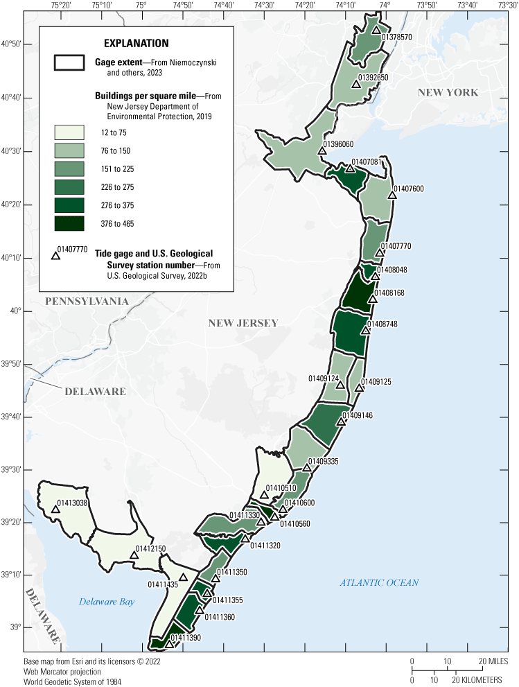
At the onset of this study, the USGS operated a network of 25 real-time tide gages (table 1) along the coast of New Jersey that recorded and transmitted 6-minute averaged tidal water-surface elevations to monitor tidal conditions (fig. 1). Expansion of the network since this project began resulted in the installation of nine additional tide gages, but these were not included within the original scope of work for this project. The New Jersey Department of Environmental Protection (NJDEP), and New Jersey Office of Emergency Management (NJOEM) partnered with the USGS to improve the effectiveness of the existing tide gage early warning network by developing a library of static flood-inundation maps for each of these 25 tide gages using the published ADvanced CIRCulation Model (ADCIRC) hydrodynamic model for FEMA Region II (Risk Assessment, Mapping, and Planning Partners, 2014a). The maps cover coastal and tidewater communities from Greenwich in Cumberland County, through New Milford in Bergen County. Concurrently, an analysis of impacts using the maps generated would be conducted at the National Weather Service (NWS) “moderate flood stage” (National Oceanic and Atmospheric Administration, 2022a) to provide a summary of effects on structures and critical infrastructure.
Table 1.
Peak-of-record tide elevations, National Weather Service (NWS) flood categories, and Federal Emergency Management Agency (FEMA) annual exceedance probability elevations (from Suro and others, 2016) at 25 U.S. Geological Survey (USGS) tide gages in New Jersey. [—Left][A, AE, VE, and unshaded X are special flood hazard zone designations. Dates shown in month/day/year. NWS, National Weather Service; NAVD 88, North American Vertical Datum of 1988; FEMA, Federal Emergency Management Agency; N.J., New Jersey; >, greater than; <, less than; —, no data gathered.]
Table 1.
Peak-of-record tide elevations, National Weather Service (NWS) flood categories, and Federal Emergency Management Agency (FEMA) annual exceedance probability elevations (from Suro and others, 2016) at 25 U.S. Geological Survey (USGS) tide gages in New Jersey. [—Right][A, AE, VE, and unshaded X are special flood hazard zone designations. Dates shown in month/day/year. NWS, National Weather Service; NAVD 88, North American Vertical Datum of 1988; FEMA, Federal Emergency Management Agency; N.J., New Jersey; >, greater than; <, less than; —, no data gathered]
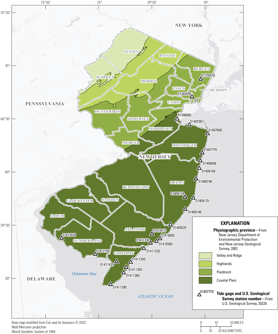
Map of U.S. Geological Survey (USGS) tide gages included in the study with overall study area extent and physiographic provinces.
Purpose and Scope
This report summarizes the development of 50 coastal flood-inundation map libraries for communities adjacent to 25 selected USGS tide gages. The purpose of these map libraries is to estimate varying degrees of flood-inundation scenarios and provide visualizations to help users understand the coastal flood risk in each area. The flood-inundation maps cover approximately 1,430 square miles of coastal, back bay, and tidewaters areas within the New Jersey counties of Cumberland, Cape May, Atlantic, Ocean, Monmouth, Middlesex, Union, Essex, Hudson, and Bergen. The maps are presented with elevations referenced to North American Vertical Datum of 1988 (NAVD 88) and are linked to recorded elevation at existing real-time tide gages. The range of mapped flood levels covered by the inundation-map libraries at each tide gage vary due to several factors including model output and unique physical characteristics of the local area. Generally, the lowest inundation map elevation for each gage corresponds with the NWS “flood stage,” which is defined as the stage at a given location when rising waters create a hazard to lives, property, or commerce (National Weather Service, 2022a). The NWS defines “moderate flooding” as the inundation of secondary roads where transfer to higher elevation may be necessary to save property and some evacuation may be required (National Weather Service, 2022b). Moderate flooding was the primary impetus and focus of this study. The upper limits of the inundation map layers for each gage were raised above NWS defined “major flooding” to the greater of either the peak recorded elevation or the 500-year flood elevation (table 1) to provide a visualization of synthetic coastal flood level scenarios for catastrophic events. The NWS defines “major flooding” as flooding that includes extensive inundation and property damage (National Weather Service, 2022c).
Although the coastal flood level scenario maps are not intended to match or replace FEMA Special Flood Hazard Area (SFHA) maps they do provide users with a better understanding of how inundation changes and impacts expand as flooding increases. This connection between these flood inundation scenario maps and real-time and historic recorded data at the USGS tide gages gives users the ability to associate current, historic, or forecasted tide gage elevation data with a visualization of estimated storm surge inundation. Incorporating hydrodynamic model output from synthetic storms, which includes localized water level effects, allows for a better understanding of the potential inundation at NWS flood elevations (fig. 2) as compared to using a more simplistic flat water-surface “bathtub” representation of storm surges.
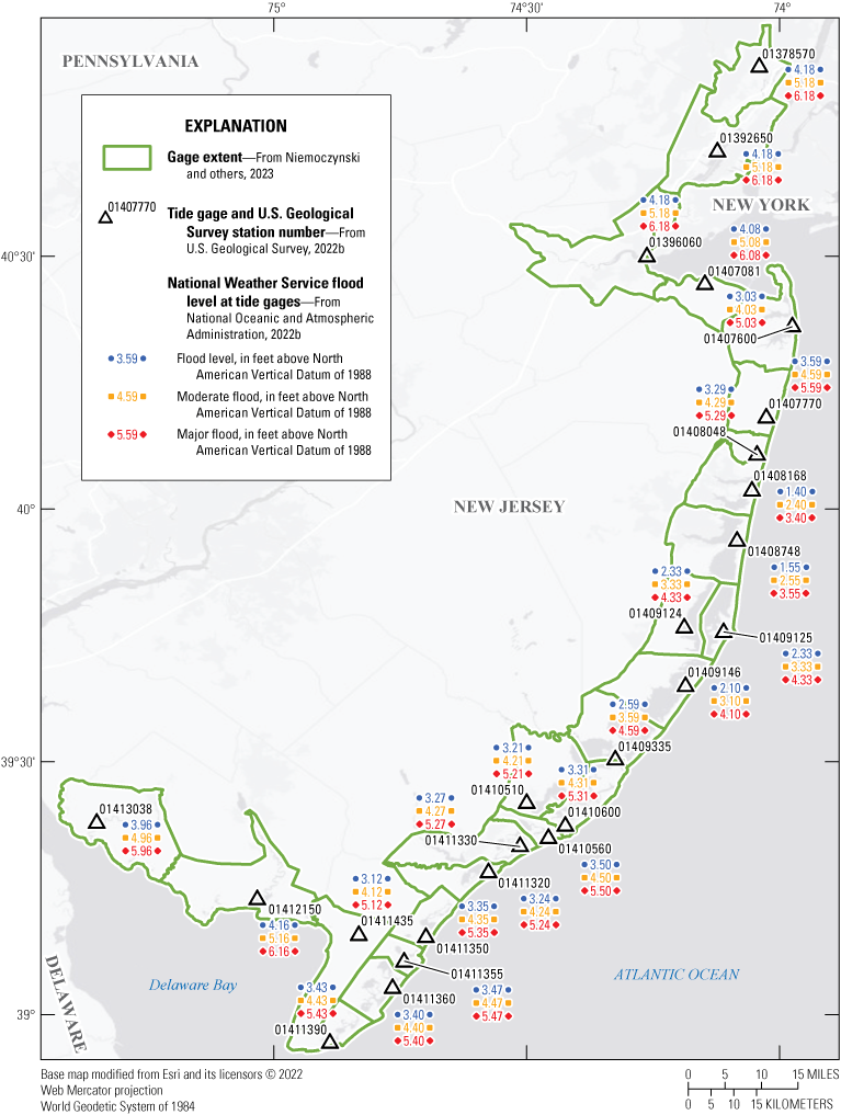
Map of U.S. Geological Survey tide gage-mapped extents and National Weather Service flood categories.
Description of Study Area
The Atlantic coastline of New Jersey is a variable landscape that transitions from highly developed, impervious areas outside the New York City metropolitan area in the counties of Bergen, Essex, Hudson, and Union to sod banks and marshy low-lying rural areas in Cape May and Cumberland counties. Within this dichotomy, other areas such as the promontory of the Atlantic highlands in Monmouth County, which have the highest elevation along the Atlantic coast south of the state of Maine, stand out as unique. The population of many of these areas experience significant ephemeral growth during the summer season which is concurrent with much of the Atlantic hurricane season (June 1 to November 30). Tropical storms and hurricanes generally pose the greatest risk of flood damage for the coastal areas of New Jersey which led in part to the development of the New Jersey Tide Telemetry Network in the 1990s. The New Jersey Water Science Center (NJWSC) network of tide gages was later renamed the New Jersey Tide Network (NJTN) as it expanded and added other types of tidal data collection. At the inception of this study in 2018, the NJTN included 25 continuous-record tide gages from Cumberland to Bergen County. Additional tide gages have been added to the network since 2018, however, this study only uses the continuous-record tide gages listed in table 1 that were active at the beginning of this project.
A mapping extent was developed for each USGS tide gage based on predicted surge extents with the intent to provide flood inundation scenario mapping for most of the coastline from Cumberland to Bergen County. The coastline of New Jersey is not a straight uniform feature and the tide gages in the NJTN are not evenly spaced which resulted in map extents that varied by tide gage. Additionally, some map extents were flagged with areas of increased uncertainty because of the distance from the USGS tide gage or complex physical features such as marsh impoundments, infrastructure, and intricate tidal waterways. Extending the mapped areas to include areas of increased uncertainty was considered a more conservative and safer approach than leaving a void in the mapping where users and management officials would need to approximate their own interpretation of flooding by another independent source. These flood-inundation scenario map extents intersect with NWS coastal forecasts, allowing users to associate real-time water level predictions at the coast with data-derived flooding scenarios inland to better understand flood risk from an approaching storm.
Previous Studies
Coastal flood studies to determine federal flood hazard insurance have been conducted since about the late 1970s which predates the establishment of FEMA. Prior to this modeling effort, many earlier studies along the coastline of New Jersey were completed and became effective in the 1980s. Currently, most New Jersey municipalities use coastal flood studies with effective dates ranging from 2003 through 2020 (fig. 3). FEMA began a new coastal analysis and mapping study in 2009 to produce updated flood insurance rate maps (FIRMs) (Risk Assessment, Mapping, and Planning Partners, 2014a). This study, the FEMA Region II Coastal Storm Surge Study, was a major undertaking. It involved a joint venture in which a few engineering consulting firms worked as contract partners with FEMA Region II. Region II includes the states of New York and New Jersey, as well as Puerto Rico and the U.S. Virgin Islands. Region II's coastal study covered all the coastal counties of New Jersey and extended beyond to include areas like the five boroughs of New York City and along the Hudson River to Troy, N. Y. The coastal counties for New Jersey are defined as those along the Atlantic Ocean and the Delaware Bay, including (from north to south): Bergen, Essex, Union, Middlesex, Monmouth, Ocean, Burlington, Atlantic, Cape May, Cumberland, and Salem.
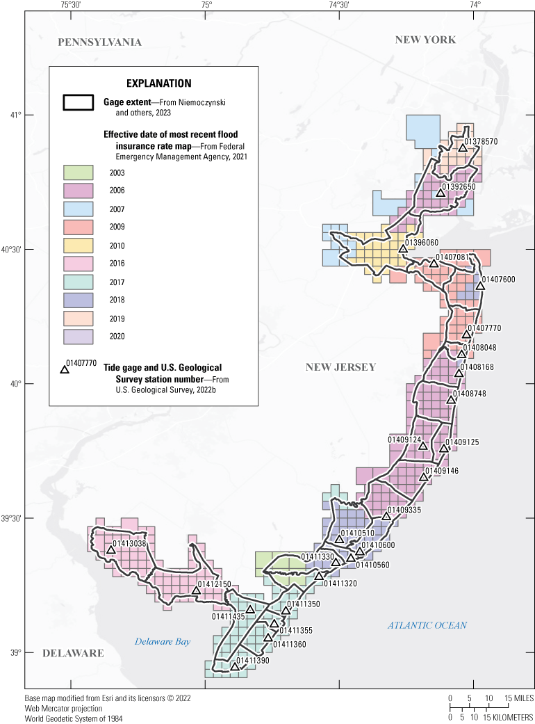
Map of Federal Emergency Management Agency Flood Insurance Study effective dates for selected coastal communities in New Jersey.
The approach for the FEMA study utilized several computer software packages, including ADvanced CIRCulation Model (ADCIRC; Luettich and others, 1992) for storm surge modeling and Simulating Waves Nearshore (SWAN) model (The SWAN Team, 2022) for overland waves analysis and probability statistics. FEMA's study would follow existing guidelines and methods from previous work, with the benefit of improved meteorological and storm data. The use of a numerical hydrodynamic model was important to expand upon the discrete storm surge data measurements and provide coverage throughout the coastal communities studied. The methods characterizing the meteorology and storm surge associated with tropical and extra tropical storms were developed and calibrated external to this inundation mapping project by FEMA and the Risk Assessment, Mapping, and Planning Partners (RAMPP) team of cooperating partners for the FEMA Region II Coastal Storm Surge Study. This inundation mapping project utilized the published modeling output generated by the RAMPP team (Risk Assessment, Mapping, and Planning Partners, 2014a) to develop coastal flood inundation maps and associated impact analysis for selected major storm simulation events as a planning and early warning tool. Utilizing the output from the hydrodynamic model was a better representation of the true storm surge water-surface relative to using generic flat “bathtub” layers to help communities and emergency managers better understand the potential hazards from storm driven surge.
Site Selection
All 25 active real-time continuous-record tide gages in the NJTN along the Atlantic coast of New Jersey and around the peninsula of Cape May were selected to have coastal storm-scenario flood inundation mapping developed. As the need for more data in tidally influenced areas along the coast continues to gain support, the NJTN continues to change and grow, but any new tide gages activated after the project began were not included in this study. Also, tidal crest-stage gages were not included in this study because they are partial record gages and do not collect continuous record tide data or transmit in real-time. The 25 selected tide gages provide tidal water-surface elevation and local meteorological data including wind speed, wind direction, barometric pressure, precipitation, relative humidity, and air temperature for a large extent of the New Jersey coastline, but they are not evenly distributed along the coast (NWIS; U.S. Geological Survey, 2022b). Variable tide gage spacing, and unique physical features associated with the back bays, tidal channels, and inlets resulted in the development of map extents customized for each tide gage (fig. 4).
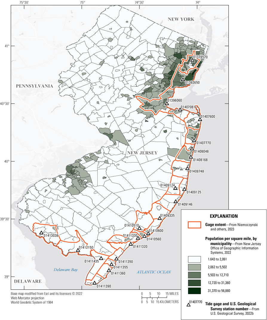
U.S. Geological Survey tide gages used in the study, outline of mapped extents, and municipalities showing variable size and distribution of major populations to gage locations.
Creation of Flood-Inundation Map Libraries
The USGS has defined standardized procedures for creating riverine flood-inundation maps for flood-prone communities (U.S. Geological Survey, 2021) to ensure consistency across different USGS offices. As this study involved coastal and tidewater flood-inundation maps using outputs from a coastal hydrodynamic model, many of the standardized procedures were not applicable. Tasks specific to the development of the coastal flood-inundation maps were, (1) acquisition of the coupled ADCIRC-SWAN hydrodynamic model outputs that were used for the FEMA Region II Coastal Storm Surge Study (Risk Assessment, Mapping, and Planning Partners, 2014a), (2) selection of applicable synthetic storms for the study area from a library of 159 modeled tropical storm scenarios, (3) extraction of modeled water-surface elevations and datum transformation using NOAA Vertical Datum Transformation Utility (VDatum; National Oceanic and Atmospheric Administration, 2022c), (4) determination of coverage extent for inundation maps for each tide gage, (5) production of estimated flood-inundation scenario maps at various tidal water-surface elevations linked to each of the 25 tide gages using a topobathymetric digital elevation model (TBDEM) within a geographic information system (GIS), and (6) preparation of the maps as 3-meter raster grids that depict the areal extent of flood inundation and depth of flood waters, per scenario for display on the USGS supported Interagency Flood Risk Management (InFRM) Flood Decision Support Toolbox (FDST) mapping website (U.S. Geological Survey, 2022a; https://webapps.usgs.gov/infrm/fdst).
Hydrologic Data
The inundation study includes data from 25 real-time tide gages with most having continuous records beginning in the late 1990s or early 2000s. Tidal water-surface elevation at each gage is averaged and recorded every six minutes, then transmitted hourly by a satellite transmitter inside the tide gage equipment shelter and made available on the internet through the USGS National Water Information System (NWIS; U.S. Geological Survey, 2022b). Elevation data from these tide gages are referenced to NAVD 88. Annual maximum tidal peaks, as well as the daily high-high and low-low tidal statistics are published at each gage in addition to the instantaneous data that are available on NWIS.
Hydrodynamic Model
The hydrodynamic model used for this study was a product of the FEMA Region II storm surge study that was initiated to produce updated FIRMs. The model is a loose coupling of the ADCIRC coastal circulation and storm surge model with the SWAN model. ADCIRC computes wind and wave driven storm surges within the region of interest and SWAN computes wind-driven wave fields (Toro and others, 2011). The combined models functioned simultaneously on an unstructured, triangular mesh grid with specific node points and is referred to as an ADCIRC-unSWAN model. Throughout the remainder of this report the combined ADCIRC and unSWAN model will be referred to simply as the ADCIRC model. The ADCIRC model simulation production runs use inputs consisting of meteorological wind and pressure files describing atmospheric conditions, model grid and static parameter files, command files for the program, and a tide “hot start” file used to begin the simulation (Risk Assessment, Mapping, and Planning Partners, 2014b). Once a simulation completes, there are several output time-series that are created. They include atmospheric pressure, wind stress or velocity, water elevation, and depth-averaged velocity for the simulation run at all nodes in the model grid from the coast and overland (Risk Assessment, Mapping, and Planning Partners, 2014b). The water elevation time-series was output on a 400-second timestep for the FEMA model used for this study and was the output used to generate the flood inundation maps described within this report. There are also two outputs generated at user designated specific recording stations for elevation times series and depth-averaged velocity time series.
To select meteorological storm characteristics for use as input for the model, the Joint-Probability Method (JPM) approach was used. In the application of the JPM, all possible combinations of storm attributes along with their probabilities are considered, followed by evaluation of the surge effects from those combinations, and calculation of probabilities associated with combinations that generate peak water-surface elevations greater than the value of interest at a location of interest (Toro and others, 2011). Five critical parameters including central pressure, radius of maximum winds, maximum wind speed, heading, and the Holland B (dimensionless parameter that controls the wind profile) are considered in the application of the JPM. Further reading on the JPM approach can be found in “Guidance for Flood Risk Analysis and Mapping: Statistical Simulation Methods” (Federal Emergency Management Agency, 2016). Results from the JPM approach were used to define and input storm impacts for the flood-inundation map scenarios, as described below.
Storm Selection
For the FEMA Region II Coastal Storm Surge Study, 159 synthetic tropical storm and 60 extratropical storm production runs were generated in ADCIRC. To generate informative flood-inundation maps that are useful to both emergency management personnel and the public, the USGS narrowed the storm scenarios down for display. Many of the simulated storms had landfall locations on the eastern end of Long Island, New York, and were not considered useful for this study (table 2). The remaining storms were ranked based on greatest potential risk for moderate to severe flooding for New Jersey coastal communities. Six storms were selected among the 25 gages where inundation maps were generated. A summary of the characteristics associated with the selected storms are listed in table 3.
Table 2.
Summary of storm selection by U.S. Geological Survey tide gage for Federal Emergency Management Agency Coastal Storm Surge Study simulated storms.[Simulated storms are from Risk Assessment, Mapping, and Planning Partners (2014b). USGS, U.S. Geological Survey; N.J., New Jersey]
Table 3.
Storm simulation characteristics at modeled landfall location or closest approach position for Federal Emergency Management Agency Coastal Storm Surge Study simulated.[Simulated storms are from Risk Assessment, Mapping, and Planning Partners (2014b). ID, identification number; N.J., New Jersey; N.Y., New York]
Storms were evaluated by examining the maximum elevation for all nodes in the model grid, known as the MAXELE file in ADCIRC. The MAXELE represents the maximum modeled water-surface elevation across all simulations at each mesh node. These nodes and associated maximum elevations were exported from ADCIRC and displayed on a map of the study area to evaluate spatial distribution of the MAXELE nodes along the New Jersey coastline (fig. 5).
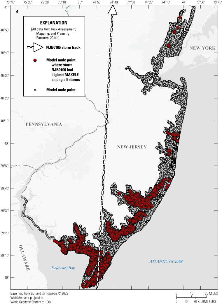
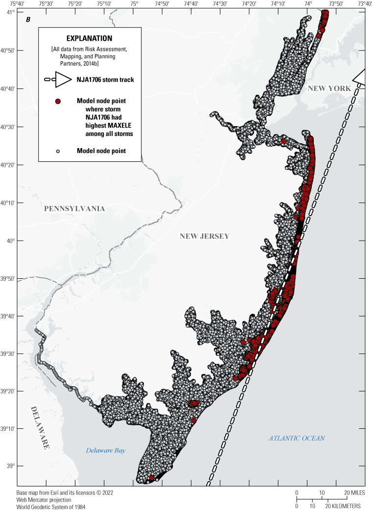
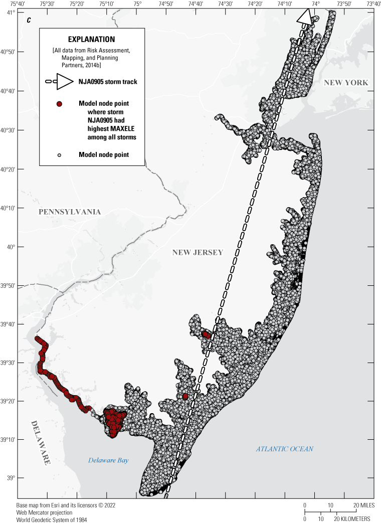
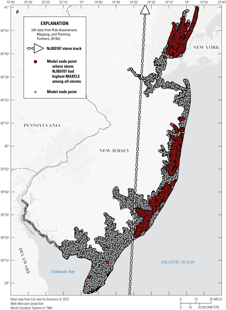
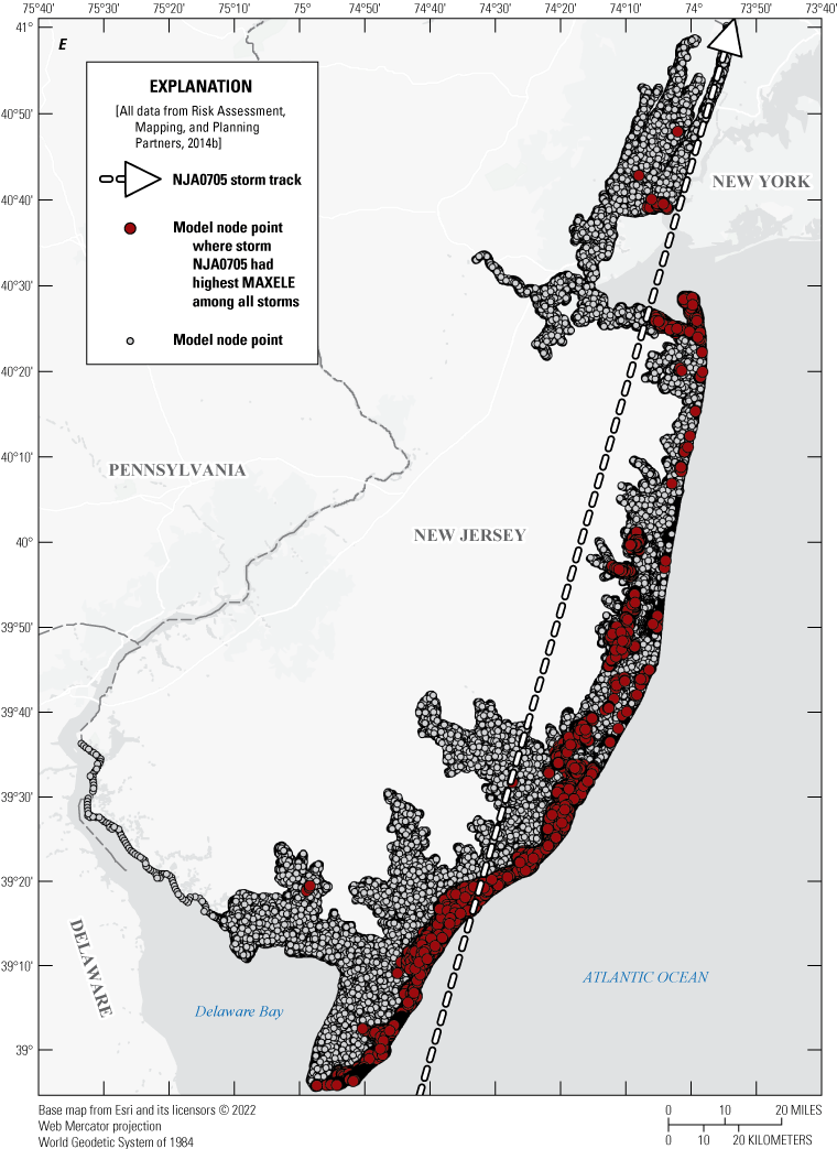
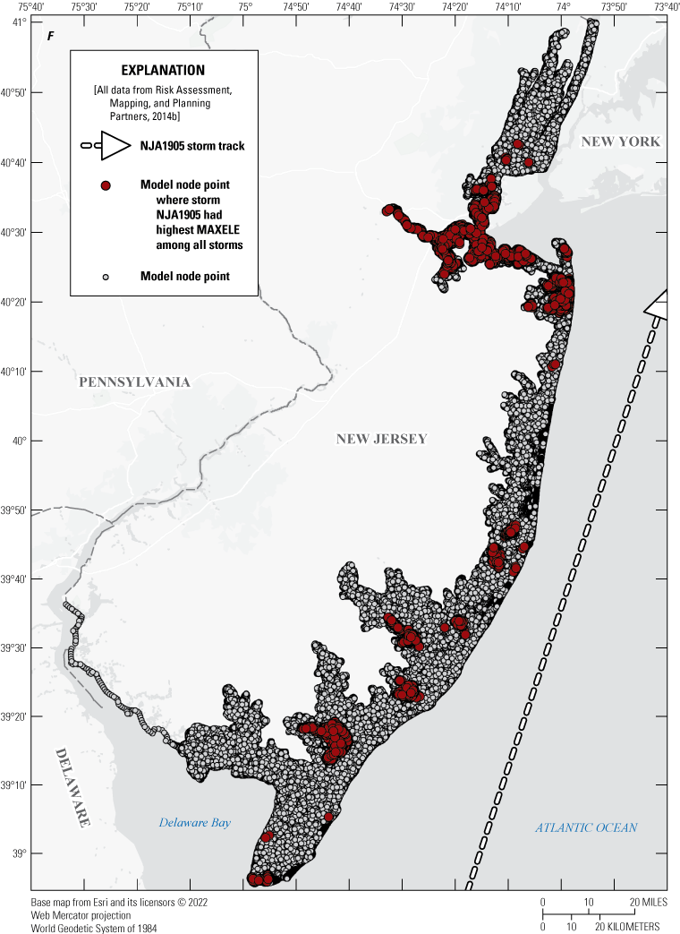
Maps showing maximum modeled water-surface elevations (MAXELE) amongst all mesh node points for six chosen storm scenarios from the Federal Emergency Management Agency hydrodynamic model (Risk Assessment, Mapping, and Planning Partners, 2014a). A, Storm scenario NJB0106, B, storm scenario NJA1706, C, storm scenario NJA0905, D, storm scenario NJB0107, E, storm scenario NJA0705, and, F, storm scenario NJA1905.
To represent scenarios with the highest risk of moderate to severe flooding, storms with the highest density coverage of MAXELE nodes were selected as the primary storm for each county. Maximum wind speed and landfall location (and, by association, wind direction) proved most relevant when evaluating the intensity of potential flooding in coastal communities and the associated MAXELE node coverages. The primary storm selected at each tide gage was named STORM A and represented a storm track that closely followed the mid-Atlantic coastline and usually made landfall near the tide gage or adjacent community. For tide gages in the northern counties (Monmouth, Middlesex, Essex, and Bergen), STORM A represented a grazing sideswipe. These were generally selected to produce simulated flood inundation scenarios that included dynamic storm surge characteristics of an overwater to overland storm track transition.
A secondary scenario called STORM B was selected to simulate flood inundation scenarios associated with a storm remaining further offshore and then making landfall in either Cape May or Atlantic counties. STORM B scenarios would be expected to produce different inundation effects based primarily on wind direction difference from the alternative storm track as well as from the final landfall approach and location. Two coastal flood inundation scenarios were presented for each tide gage to illustrate the variability in storm surge flooding from distinctions in storm characteristics and local geography. It was decided, presenting more than two flood inundation scenarios could add confusion and limit use and understanding of these early warning and mitigation tools. In addition, the study did not combine flood inundation scenarios from multiple storms to preserve the unique differences generated by tidal and meteorological model forcing parameters as an attempt to illustrate the non-uniform and dynamic nature of many coastal storm surge events.
Tide Gage Flood Inundation Extents and Areas of Uncertainty
Given the complex nature of tidal hydrodynamics near the inlets and back bay systems of New Jersey, the distance from a tide gage where coastal flood inundation can be reliably predicted is variable and generally unknown in the absence of specific, fine-resolution modeling. Traditional riverine flood inundation mapping is less complex because typical streamflow in rivers and streams is generally controlled by the shape, slope, and channel roughness. Flood inundation mapping along river reaches also benefits from calibration to stream flows that have been measured by direct or indirect methods and used to calibrate the associated step-backwater or other type of hydraulic model. The flood inundation maps produced in this study required developing an understanding between the behavior of the modeled water-surface elevation at the existing USGS tide gage and other locations within the potential extents of mapping for each tide gage.
The flood-inundation extents for each tide gage define the boundary for displaying the flood-inundation maps. Several procedures were employed to generate and tune the extents. Preliminary map extents were created in GIS by clipping ADCIRC node points and New Jersey Parcels (New Jersey Office of Geographic Information Systems, 2018) to each county. Polygons were aggregated at a 200-meter (m) scale then manually edited to remove holes in the polygon whose minimum bounding rectangle had a long axis smaller than 250 feet (ft). The remaining polygons were dissolved into one polygon per tide gage as the initial attempt at delineating mapping extents. In this study, flood inundation extents define the boundary determined for displaying inundation maps for each tide gage that would provide the recorded or reference tidal water-surface elevation data. Initial flood inundation extents were manually evaluated to remove areas that were hydraulicly disconnected, or otherwise outside of tidally affected areas. At other locations the potential map extents were reduced or eliminated because of large distances from the tide gage or closest ADCIRC node points. It was unclear if the water-surface elevations within these areas would respond consistently or remain hydraulicly connected to the forces affecting the water-surface elevation at the tide gage, so it was determined the most appropriate action was to remove those areas from the mapped extents. Inland areas were manually trimmed at major roadways, where applicable, or again at areas that stretched far beyond available model node points. Defining the flooding extents based on nearby USGS tide gages, allows for measured tidal water-surface elevations at the tide gage to be compared to simulated inundation water-surfaces at the tide gage, and the corresponding simulated flooding extent, for forecasting and visualizing inundation in communities.
A warning was created for some tide gage map extents to alert users if the relation between the near tide gage hydrodynamics and an area within the mapped extents may be less accurate than others. In these cases, a flag for areas of increased uncertainty was developed and is displayed on maps in the FDST viewer. Where appropriate, the flags mark locations where there is a lack of node points, DEM data may appear unreliable, or existing physical features such as impoundments in marsh areas may add unknown uncertainty to the modeled output. In some circumstances limited areas of inundation within a station extent were noted to respond inconsistently between increasing levels of inundation, possibly owing to temporal differences in the modeled water surfaces as the simulated storm moves through the area. Examples of this would include a limited area of the inundation grids showing significant inundation at the 4-foot level, but then “receding” when the 5- and 5.5-foot level was overlaid, followed by once again being inundated in the 6-foot and higher inundation levels. These areas were also designated with the flag for increased uncertainty. Gages that utilized these flags for areas of increased uncertainty included Maurice River at Bivalve, Sluice Creek at South Dennis, Cape May Harbor at Cape May, Ludlum Thorofare at Sea Isle City, Great Egg Harbor Bay at Ocean City, Absecon Creek at Absecon, East Thorofare at Ship Bottom, Barnegat Bay at Route 37 Bridge near Bay Shore, Barnegat Bay at Mantoloking, Watson Creek at Manasquan, Shrewsbury River at Sea Bright, Raritan Bay at Keansburg, Newark Bay at Passaic Valley Sewerage Commission (PVSC) at Newark, and Hackensack River at Hackensack, N.J.
Topographic and Bathymetry Data
To ensure proper representation of overland flow, a topobathymetric digital elevation model (TBDEM) from the USGS Coastal National Elevation Database (CoNED) Applications Project was utilized to generate inundation layers and depth grids (Danielson and others, 2018). CoNED TBDEMs are constructed from multisource topographic and bathymetric data that are aligned vertically and horizontally to a common reference system (Danielson and others, 2018). This hydro-enforced TBDEM represented most bridges over navigable waterways as having their bridge decks removed, thus reflecting an elevation representative of the bathymetry of the associated waterway. These bridges are displayed as inundated at all levels of water-surface elevation. Some smaller bridges and culverts were not “removed” from the hydro-enforced TBDEM and will display the actual elevation of the bridge deck relative to the water surface until the bridge deck physically becomes inundated by the rising water-surface elevation.
Data Output and Adjustment
Hydrodynamic data from the FEMA Region II Coastal Storm Surge Study were provided to the USGS in the form of ADCIRC model output files which were accessed and queried through the Surface-water Modeling System (SMS). This study accepted the model calibration and verification performed by FEMA Region II and its contractors and utilized the final output for map development. Model simulations for the Region II study were run for 72 hours with storm forcing increased or “ramped” during the first 12 hours. This project primarily focused on generating maps of flood inundation resulting from various selected storm scenarios, so data output from the model ramp-up period, when initial forcings were not directly impacting the New Jersey coastline, were excluded from processing for this study. The simulation data used to generate inundation maps were extracted for all New Jersey node points approximately 24 hours before landfall through the end of the simulation for an average of 48 hours. Of the large sample of node points in the FEMA Region II study ADCIRC and unSWAN mesh file, only those that fell within a buffered polygon shapefile of New Jersey were extracted. Simulation data were output from SMS as text and formatted for input into ArcGIS and Python geoprocessing scripts.
Model simulation data were output in meters, vertically referenced to the mean sea level (MSL) tidal datum, so a transformation to the USGS standard of NAVD 88 in feet was required. Where possible, VDatum was used to vertically transform the data to NAVD 88 (fig. 6). For some gages, there were areas where transformation data for a reference tidal datum did not exist, mainly farther away from the coast and in tidal back bays or marshy areas. In these instances, a conversion factor was generated based on all points in the tide gage station extent where transformation was possible and used to approximate a transformation at points outside the area of VDatum. The conversion factor was calculated using equation 1, where the average conversion factor, cavg, computed for the points within the map extent of each tide gage where VDatum was applicable, was added to the MSL water-surface elevation.
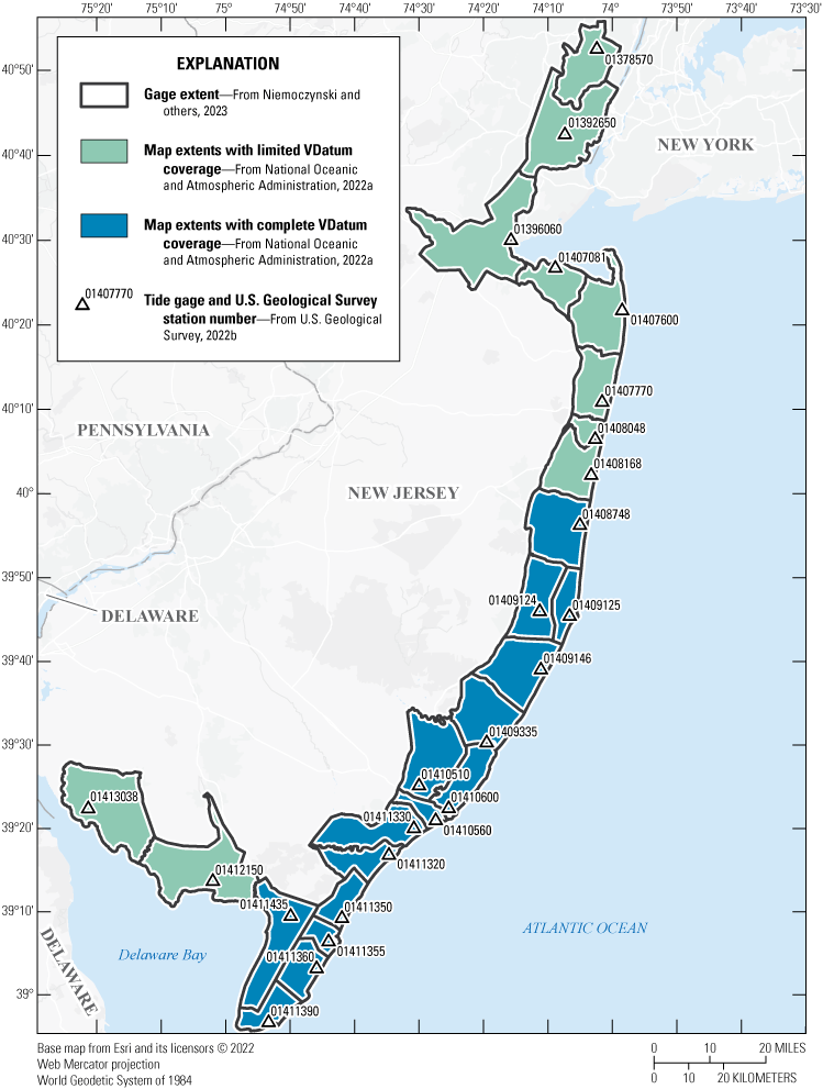
Map of coastal areas with Vertical Datum Transformation Utility (VDatum) coverage. Green areas of the figure represent tide gage extents where an average conversion factor was used in place of VDatum coverage.
WSELft NAVD88
is the water-surface elevation in feet NAVD 88;
WSELft MSL
is the water-surface elevation in MSL converted to feet;
cavg
is the average of c calculated for each transformable node point in the station extent; and
N
is the number of node points where VDatum was applicable.
For gages where use of cavg was necessary, the value of cavg was compared to the nearest NOAA tide gage with an existing MSL to NAVD 88 transformation to ensure the calculated value was reasonable. An example is shown in figure 7, using gage 01396060 Arthur Kill at Perth Amboy, N.J., and a single timestep in storm NJB0107, where only 43 percent of node points in the mapping extent with non-null values could be transformed by VDatum and yielded a cavg of 0.092 ft (standard deviation 0.04 ft). NOAA gage 8531545 Keyport, Raritan Bay N.J., approximately 5 miles southeast, has a published vertical transformation value of 0.10 ft (National Oceanic and Atmospheric Administration, 2022b).
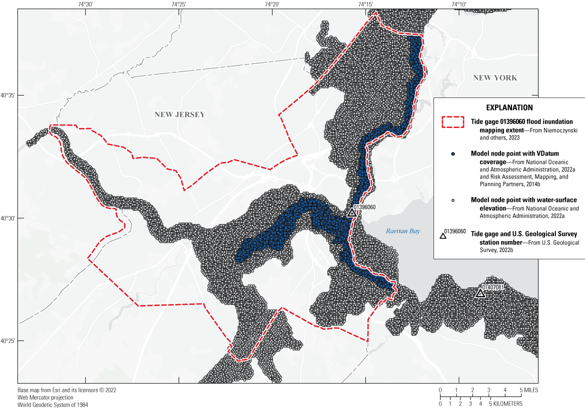
Example of limited Vertical Datum Transformation Utility (VDatum) coverage at U.S. Geological Survey tide gage 01396060 Arthur Kill at Perth Amboy, New Jersey for storm NJB0107.
Development of Flood-Inundation Maps
Once the hydrodynamic model output was converted to NAVD 88, time step, node latitude and longitude, and water-surface elevation were converted to individual point coverages. For each point coverage, a subset of points was selected based on the relevant tide gage station extent and a water-surface elevation raster dataset was interpolated with a 3-meter cell size using Esri’s Topo to Raster tool (Esri, 2021). The tool was run with the datatype parameter set to “Spot” optimizing the method for point data input instead of contour data input. This selection alters the default values for the roughness penalty and tolerance parameters, but otherwise the tool was run with default parameter values. After generation, each interpolated water-surface raster dataset was sampled at the grid point nearest the tide gage locations to generate a simulated hydrograph for the selected storm at the tide gage in feet NAVD 88 (fig. 8).
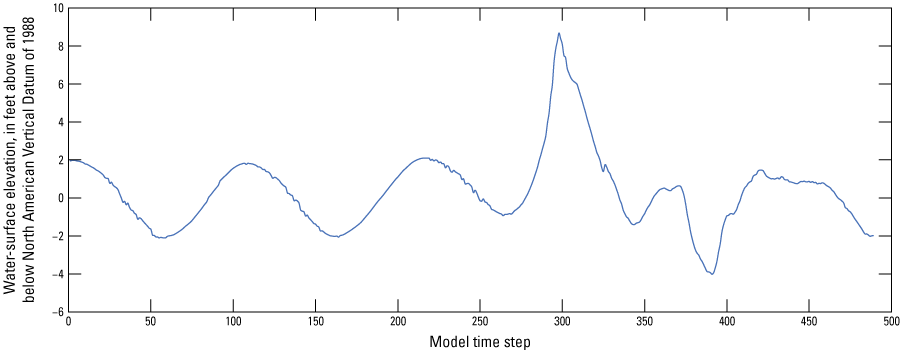
Example Water-surface Elevation Hydrograph at tide gage 01411390 Cape May Harbor at Cape May, New Jersey for storm NJA0705.
Timesteps in the hydrograph were matched with a list of target tide gage readings in half-foot increments ranging from 1.5 ft to the 1-percent annual exceedance probability elevation. The hydrographs were also aligned with the NWS flood stages at the tide gages. Only timesteps preceding the maximum water-surface elevation value were evaluated and labeled as follows:
-
“Exist”: a timestep exists with a tide gage reading within 0.2 ft of the target;
-
“Inter”: no timestep exists within 0.2 ft, but the target value is between two timesteps; and
-
“Bathtub”: the target value is above the maximum value in the hydrograph.
Organizing the timesteps into these three categories allowed for more efficient processing of the data. Matches labeled “Exist” were ready for generating depth grids and needed no additional processing, but those labeled “Inter” and “Bathtub” required additional processing to generate the missing water-surface datasets.
For matches labeled “Inter,” a new water-surface raster dataset was created using Esri’s Cell Statistics tool. Each cell value in the new raster was the maximum between cell values in the water-surface raster datasets with tide gage readings just below and just above the target value. The newly generated raster dataset represented a “worst case” of flood inundation based on the available simulation data. Some storm scenarios showed a rapid rise in water-surface elevation exceeding 0.5 ft per timestep at a tide gage which resulted in the creation of duplicate water-surface raster datasets. Additionally, duplicates arose from NWS flood stages being close to the 0.5 ft target, for example 4.4 ft versus 4.5 ft. Duplicates were removed from further processing.
For matches labeled “Bathtub,” a new water-surface raster dataset was created using Esri’s Raster Calculator. The difference between the target value and the maximum recorded value in the hydrograph was added to each cell in the water-surface raster dataset corresponding to the maximum value. This raster represented a “hybrid bathtub” surface that artificially raised the maximum storm-forced surface to the target tide gage reading. The term “bathtub” is often used when generating a water-surface elevation that represents a single elevation and is essentially flat like water in a bathtub. In this study the term “hybrid bathtub” was selected to describe the method of offsetting each node in the water-surface elevation raster by a fixed value. The resulting water surface is not flat like a typical bathtub surface. It matched the shape and contour of the modeled timestep surface but with a fixed offset (bathtub value) added to each raster value. “Bathtub” layers were generated at whole foot increments only.
All the raster datasets, regardless of generation method, were converted into depth grids by subtracting the TBDEM in feet NAVD 88 from the water-surface elevation raster datasets using Esri’s Minus tool. A reclassified raster dataset was created for each depth grid where water depths less than 0.1 ft were changed to 0 and removed, and values greater than 0.1 ft were changed to 1 and converted to a polygon for review and quality assurance.
Quality Assurance
Manual quality assurance of each inundated area at all tide gages was required to assess hydrologic connectivity to ocean or back bays and evaluate the topographic complexities present in coastal hydrologic systems. Inundated areas that were detached from the coastal waters were examined to identify connections with the ocean and tidal tributaries, such as over dunes, or through culverts under roadways. If the connections were deemed reasonable through review of the aerial orthoimagery, the disconnected areas of inundation were retained. Some of these were very easy to identify as the orthoimagery displayed open marsh type land cover that reflected frequent tidal inundation. Other areas were less clear, as was the case for several impoundments found within the station extents in the Monmouth County tide gages. For example, Deal Lake controls the level of the impoundment using a hydraulic flume structure that drains to the ocean. Specific elevations for the hydraulic structure were not obtained. Within the inundation layers, it was decided to retain the lake as “inundated” once the generated polygon displayed it as inundated despite it being slightly disconnected from the main inundation grids, as the possibility of inundation from the ocean through the flume structure exists. Disconnected polygons that are adjacent to another inundation map extent were compared with the adjacent inundation layers of similar gage heights to determine possible connectivity. If inundation was identified at a similar gage height on the adjacent map extent, the apparent “disconnected” polygon was retained. All disconnected areas of the inundation polygons determined to be erroneously delineated were removed.
After manual review and editing of the flood-inundation polygons, they were arranged in a map library designated by gage number and storm scenario identifier and run through a final processing routine to enhance the display of the final layers. The routine includes two geoprocessing steps using GIS python tools. First, each polygon is run through a tool with the default parameters set to fill small gaps inside larger polygons. Most of the gaps are artifacts from converting the raster dataset into a polygon. Second, the arranged polygons are run sequentially through a tool that calculates overlap between the inundation polygons. Taking a “lower” and a “higher” input, the tool creates an overlap polygon only where inundation from the lower tide gage reading extends beyond that of the higher tide gage reading. If an overlap exists, it is merged with the higher gage reading polygon, which ultimately becomes the next lower gage reading in the sequence. In this manner, the final polygons only show an expanding inundated area as gage readings increase and favors the “worst case” interpretation of the simulated storm data. These final polygons are then used to extract final depth grids from their respective progenitor raster datasets, with overlap polygon area extracting from the next lower raster dataset, and any “NODATA” or negative values replaced with 0.1 ft.
Evaluating Model Accuracy and Applicability
Four of the historical extratropical storm simulations modeled for FEMA's Coastal Storm Surge Study included time periods when modeled data overlapped with the period-of-record at the USGS tide gages. These extratropical simulations included nor'easters from October 25, 2005, April 16, 2007, May 12, 2008, and November 13, 2009. The latest simulation from November 13, 2009, was selected to compare against historical recorded tide data at several tide gages throughout the study area. An example in figure 9 shows modeled versus historical tide elevation data at USGS station 01411390 Cape May Harbor at Cape May, New Jersey. The modeled data showed generally consistent patterns with historical data throughout the tidal signature leading up to the event with peaks and valleys aligned (fig. 9). Some differences would be expected as the nature of the model mesh resolution results in some deficiency in capturing complexities within harbors and narrow channels (Risk Assessment, Mapping, and Planning Partners, 2014c). Specific differences between modeled and historical amplitudes were not calculated as part of this comparison. The simulated peak for the event matched the historical peak with a reasonable difference of approximately 1 ft. Differences less than 2 ft generally indicated good agreement within a study area (Risk Assessment, Mapping, and Planning Partners, 2014c).
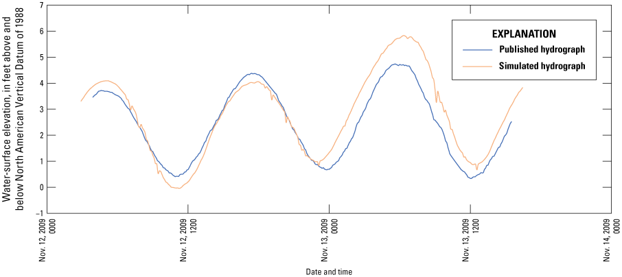
Modeled hydrograph from extratropical model production run “Winter Storm 20091113” versus historical hydrograph from U.S. Geological Survey tide gage 01411390 Cape May Harbor at Cape May, New Jersey (U.S. Geological Survey, 2022b). Time is presented in military time.
Generated inundation extents were overlaid with FEMA 1-percent annual flood hazard and 0.2 percent annual flood hazard zones in figure 10 to ensure the modeled inundation layers were not grossly underpredicting or overpredicting inundation extent within communities. To accomplish this, the finalized flood inundation polygon at a gage elevation closely representing the published Base Flood Elevation (BFE) at the gage location was selected for comparison. An example of this process using USGS tide gage 01411390 Cape May Harbor at Cape May, N.J., is provided below.

Map of U.S. Geological Survey tide gage locations, mapped station extents, and Federal Emergency Management Agency Special Flood Hazard Areas.
Referencing the most recent FIRM panel 34009C0284F for the City of Cape May, the gage location is compared to adjacent BFEs. The BFE for the actual gage location (on a pier) places it within a VE zone, which sets the BFE to 11 feet NAVD 88. FEMA V and VE Zones are areas along coasts within the FEMA-designated Special Flood Hazard Area subject to additional hazards associated with storm-induced waves (Federal Emergency Management Agency, 2021a). Although the USGS tide gage is within the VE Zone, the tidal water-surface elevations recorded by the gage use a combination of physical means, such as baffling disks in the gage well, as well as averaging algorithms applied to the raw unbaffled recorded data to filter the effects of wave action so the resulting data are more representative of still-water elevations. In addition, the model output used to generate inundation layers for this project does not include waves modeled on top of the still-water tidal elevations. In general, comparison to V and VE Zones was not considered for this project, and thus, the adjacent AE Zone or coastal AE Zone elevation was selected instead of the VE Zone BFE where applicable for comparison to the modeled inundation layers. The AE Zone is the base floodplain within the Special Flood Hazard Area where BFEs are available. In the described example for Cape May, an elevation of 8 feet NAVD 88 was used from the adjacent AE Zone. Using this information, the 8-ft inundation layer for the gage at Cape May was selected for comparison to the FEMA flood hazard zone extents.
Comparison of the FEMA zones versus the modeled inundation layers was a qualitative process focused on ensuring general consistency and identifying anomalies. Anomalies could present as regions within a station extent that show inundation extending well beyond the 0.2-percent flood hazard zone, or areas where inundation does not fill in a large portion of the 1-percent flood hazard zone. Anomalies such as these would suggest enhanced uncertainty within the modeled layers requiring delineation on the finalized map libraries and associated online mapper. Generally, the modeled inundation layers were consistent with the boundaries defined by the FEMA 1- and 0.2-percent annual flood hazard layers.
It should be noted that not all areas of the coast reflect updated, digitized flood hazard maps. Direct comparison in these areas is more challenging and, therefore, was not performed. Examples of communities without updated digitized flood hazard maps include Ventnor City and Atlantic City, N.J. More information on FEMA effective study dates can be found at the FEMA Flood Map Service Center (Federal Emergency Management Agency, 2021b).
Evaluating Community Impacts at Moderate Flood Levels
Moderate flooding, or what has been referred to as “moderate flood level” or “moderate flood stage” has generally been defined at the local governmental level and influenced by officials in each community to help identify when widespread flooding of roadways and structures begins, transportation routes become impassable, and risk to life and property starts to become a major concern. Understanding how communities are impacted by inundation from coastal flood waters associated with moderate flooding is important information necessary for local officials tasked with protection and resiliency. In the following sections the variability of impacts resulting from simulated flood levels are described and compared.
Understanding Community Size and Density
An analysis was done using simulated inundation maps referenced to water-surface elevations at the selected USGS tide gages used in this study. The simulated coastal flooding layer closest in elevation to the selected NWS flood stages (moderate or major) was evaluated to estimate the community impacts, where available. It is difficult to estimate or predict the presence or movement of people in each community so the total number of buildings (referred to in FEMA Hazus analysis as total building stock) was used as a surrogate for the general percent of people exposed to inundation. To quantify the degree of community impact, the analysis tried to identify buildings with a high likelihood of inundation and major roads and bridges that potentially experienced disruption of access due to inundation from coastal flood waters. At moderate flood stage, disruption of access to major roads and bridges was considered a high impact because it was assumed to disrupt connectivity between barrier islands and the mainland. This infrastructure is critical for moving people and assets out of potentially dangerous coastal flood areas. If access to these transportation routes is compromised at the moderate flood stage, it is assumed evacuation during major flooding events would be even more difficult and dangerous. The total area and depth of inundation for communities near USGS tide gages were also evaluated as characteristics to help quantify the community impact. Comparing the change in magnitude of total buildings and major roads potentially inundated at moderate to major flooding provides important planning, mitigation, and response information to help community, state, and federal managers increase resiliency and reduce the loss of life and property.
The community impact analysis used the extent and depth of inundation estimated from two selected synthetic storms, described earlier in this report, for the mapped extents associated with each USGS tide gage and compared them with building and major road information to evaluate flooding impacts. The area of mapped extents for each tide gage is referred to as station extents and are generally not consistent in size because of the natural irregular shape, geography, and land use properties of the New Jersey coastline. The use of percentages in categories like “total building stock inundated” are presented to describe the degree of impact because the use of totals or totals by category would be more difficult to compare. For example, figure 11 shows the total number of buildings for each station extent and the number of buildings greater than 2,000 square feet in the same extent to illustrate the variability in inundation between station extents. An initial comparison of total area, percent of area classified as urban, total number of buildings (building stock), and building size greater than 2,000 square feet, was done to develop a baseline understanding of community variability before evaluating area inundated. The total area and area classified as urban for each station extent are shown in figure 12.
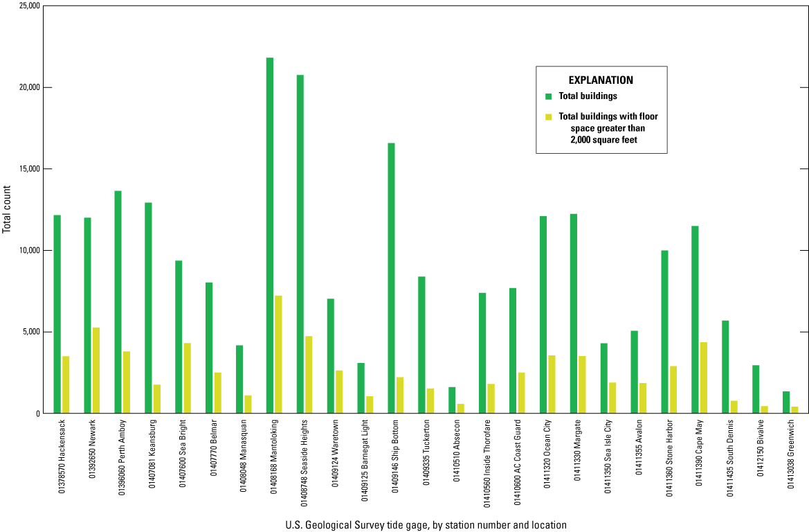
Graph of New Jersey tide gages with total building counts and buildings with floor space greater than 2,000 square feet for each station extent.
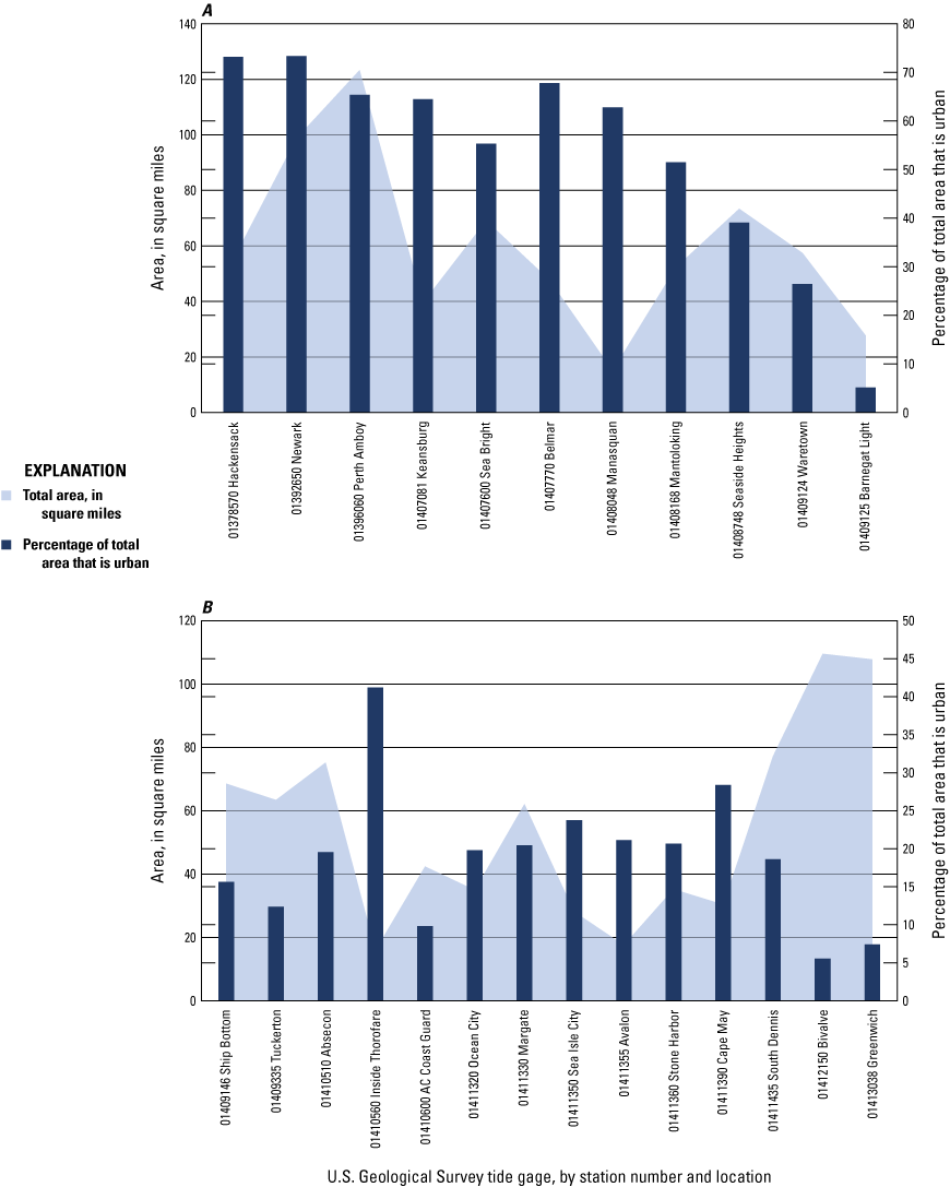
Graphs of total area in square miles and percent of area classified as urban for each station extent. A, Eleven stations, station numbers between 01378570 and 01409125. B, Fourteen stations, station numbers between 01409146 and 01413038.
The station extents for the USGS Mantoloking (01408168) and Seaside Heights (01408748) tide gages have the largest number of building structures per mapped area in the study with more than 20,000 structures per station extents. These areas include communities such as Mantoloking, Toms River, Lavallette, and Seaside Heights. Although these station extents have the largest number of structures, neither of these areas are in the top three largest areas in the study. Additional analysis of building structure data shows neither area associated with the Mantoloking and Bay Shore tide gages have the highest density of building structures in the study, but collectively they all rank in the top half of all station extents. Understanding the variability of building density among station extents may provide additional information to better assess impacts to people and property when compared to simply looking at total area or building count in a station extent. Figure 13 shows the distribution of building density among mapped station extents. As indicated earlier, the Mantoloking and Bay Shore station extents had the highest total building counts, but when analyzed for building density Mantoloking had the second highest building density and Bay Shore was not in the top 5 highest densities. Mantoloking station extent also was not in the top 5 largest areas or top 5 highest percentages of urbanized areas. Further investigation into the community characteristics highlighted, for example, that evaluating total building count and building density for mapped station extents helps show a potentially greater community exposure and impact if inundated by one of the storm scenarios when compared to some areas that may have a larger area of inundation.
Map of building density per square mile for all U.S. Geological Survey tide gage station extents.
Understanding Moderate Flooding on Buildings and Major Roads
The extents and depth of moderate flooding for the community impact analysis evaluated the impacts from scenarios STORM A and B described in this study. Understanding the count and density of homes in the mapped station extents associated with each tide gage provided better information to help evaluate the potential community impacts from coastal flooding than simply relying on the size of the area. Adding information about first flood elevations and estimated depth of flooding at each structure and along major roads allowed for a more advanced understanding of the potential severity of impacts to the residence of the community and their ability to evacuate or reach safe shelter.
Major roads were defined as roads in classes 1 through 6 in the “route_subtype” field within the New Jersey Department of Transportation (NJDOT) Roadway Network geospatial data (New Jersey Department of Transportation, 2021). These roads typically included interstates down to major county roads. The NJDEP building footprint dataset (New Jersey Department of Environmental Protection, 2019) was used to define first-floor elevations, lowest adjacent grade (LAG), and highest adjacent grade, and if the structure type was classified as critical (CS). A building’s structure was considered inundated at moderate flooding if the water-surface elevation was computed to be greater than the LAG elevation using the selected inundation layer for moderate flood stage. The water-surface elevation at each structure was determined by selecting the cell within the structure footprint with the maximum elevation.
At bridge crossings, a slightly modified approach was needed. At some bridges along major roads or over causeways, inlets, and back bay water bodies, the bridge structure can be arched or have a higher deck and low steel elevation near the center of the span when compared to the elevation at the abutments. In other situations, the bridge deck may remain above flood levels regardless of an arch or curvature to the bridge deck, but the approaching roadway becomes inundated cutting off safe access to the bridge. This potentially more complex situation was solved by combining the approaching roadway and the bridge into a single feature so they could be analyzed together. If either the bridge becomes inundated or any part of the approaching access roadway, the bridge is determined to be inundated and added to the list of impacted structures. As previously mentioned, the hydro-enforced TBDEM used for this study had many bridge decks already removed from the elevation model. For the analysis portion of this study these bridges were represented by an approach feature, as otherwise, they would always calculate as “inundated.”
Evaluating the impacts of moderate flooding required selecting coastal flood inundation layers closest to the NWS moderate flood level elevation, converted from mean lower low water (MLLW) to NAVD 88, and intersecting them with the buildings and road datasets to calculate what structures were identified as inundated. As described earlier, relying solely on total counts of structures inundated makes comparisons between communities or mapped station extents more difficult. The impact in some communities is more straightforward because they are established at a generally lower elevation, so many of the total structures are inundated at moderate flooding. In these areas, elevation, early warning, and evacuation are typically part of the strategy. In other areas, a smaller number of total structures may be inundated. However, if strategic areas and major access roads are inundated, a larger percentage of the community can be impacted. Without that vital infrastructure, the community’s ability to evacuate or access a bridge to the mainland will likely be cut off, even if their building structure or home was not inundated. One example of this is along the northern end of the Mantoloking station extents. Although the total percentage of the station extents inundated is not the highest among the mapped tide gage station extents, it does have the highest total number of buildings. As a tidal storm surge reaches moderate flooding, many buildings from Mantoloking North to Point Pleasant Beach may be cut off from accessing Route 35, Ocean Avenue, Ocean Road (Route 88), and other roads that can be used by those that would be otherwise trapped between back bay inundation and the barrier island dunes. This example is illustrated in figure 14. To better understand the magnitude of potential damage, this study looked beyond the initial analysis of building structures simply being inundated during moderate flooding by computing the depth of flooding at each structure and dividing the results into two categories: (1) the percent of structures inundated with 1 foot or more of flood water above the first-floor elevation; and (2) those inundated with 3 ft or more of flood water above the first-floor elevation at moderate flood stage. The percent of structures identified as inundated with greater than 1 ft and greater than 3 ft of flood waters during the moderate flooding scenarios for each tide gage are illustrated in figure 15.
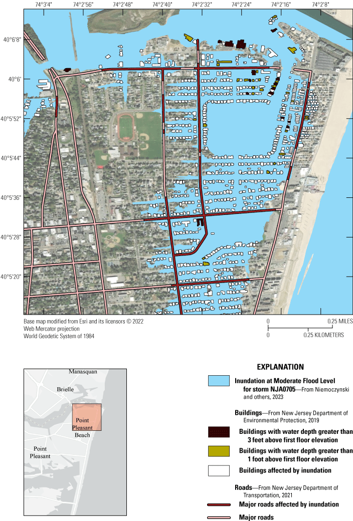
Enlarged inundation map showing moderate flooding at tide gage 01408168 Barnegat Bay at Mantoloking, New Jersey.
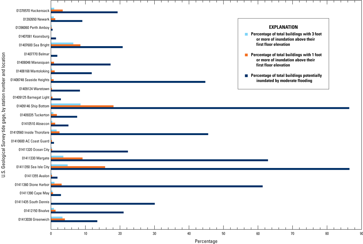
Graph showing percent of building structures inundated at moderate flooding by mapped tide gage station extents.
The evaluation of total building counts, percentage inundated, and depth of inundation for structures at moderate flood stage provides data to begin evaluating the combined impacts of coastal flooding on communities within the mapped station extents. Analyzing the compound effect of inundation to building structures, disrupted access to major roads, and damage or impact escalation from forecast error presents a comprehensive outlook of overall coastal community flood impacts. The next section of this report provides more information about this compound analysis.
Understanding Community Risk Variability from Moderate Coastal Flooding
The coastal communities covered by these new coastal flood inundation maps extend from Hackensack, Perth Amboy, and Keansburg along the northern coast to Atlantic City, Stone Harbor, and Cape May at the southern end of the New Jersey coastline. Moderate flooding has generally been defined as when widespread flooding of roadways and structures begins, transportation routes become impassable, and risk to life and property starts to become a major concern. Utilizing both coastal storm scenarios used in this study, the range of building structures impacted at moderate flood stage for each station extent ranged from more than 14,000 structures to less than 100. Figure 16 depicts some of the differences visualized with structure inundation at a moderate flood stage of 3 ft between the gages at Mantoloking and Bayshore. A structure was considered inundated if one cell from the moderate flood stage layer intersected the building footprint with an elevation above the LAG for that structure. The average percentage of structures estimated to be inundated at moderate flood stage was slightly more than 5 percent when using an average of the two storm scenarios. Several communities were estimated as having more than 20 to nearly 50 percent of the buildings inundated using the same averaged criteria while two communities stand out with estimates of more than 80 percent of the buildings inundated using the same two storm average criteria (fig. 15). The percent of these structures estimated to be inundated by 1 ft or more above the first-floor elevation ranged from nearly zero to almost 20 percent in the communities of Sea Isle City and Ship Bottom.
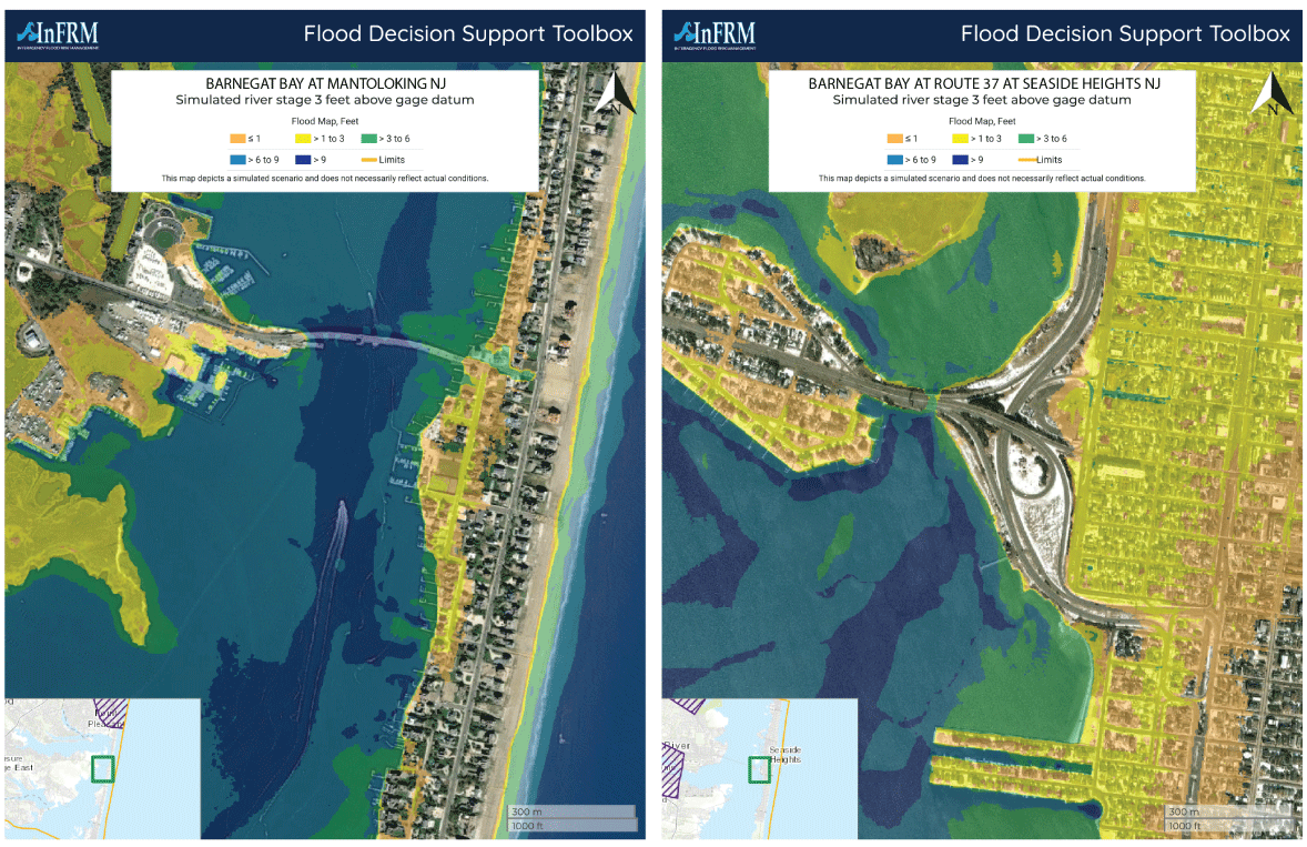
Maps showing examples of two communities—one with minimal structures inundated and another with more than 20 percent inundated.
Along with building structures, the percentage of major roads and bridges in the station extents for each tide gage were evaluated. At moderate flood stage the mean percentage of major roads affected by flooding was almost 7 percent. A few station extents indicated more than 15 percent of major roadways affected by flooding and one community exceeded 30 percent of major roadways affected. When the flood stage was increased to NWS major flood stage, the mean percentage of major roadways affected by station extents increased to slightly more than 11 percent (fig. 17A). The combined impact from flooding on building structures and major roads presents a comprehensive dataset to help evaluate the impact on coastal communities from coastal storms.
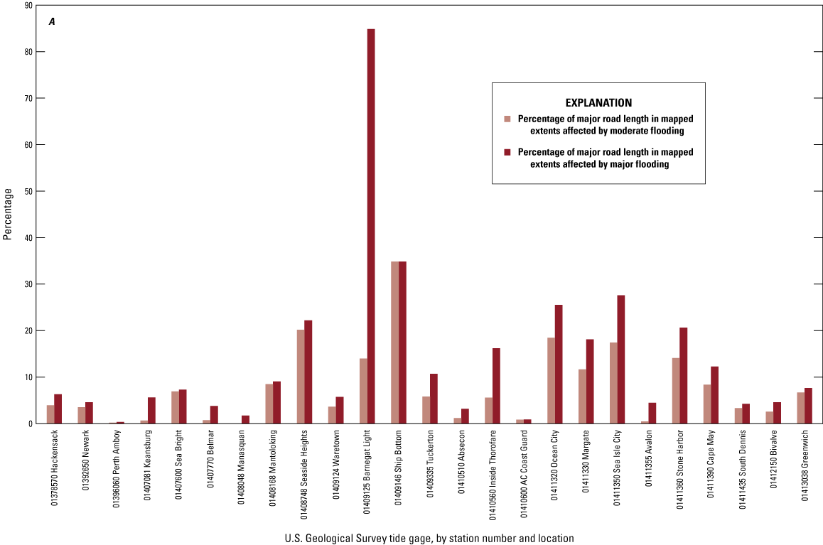
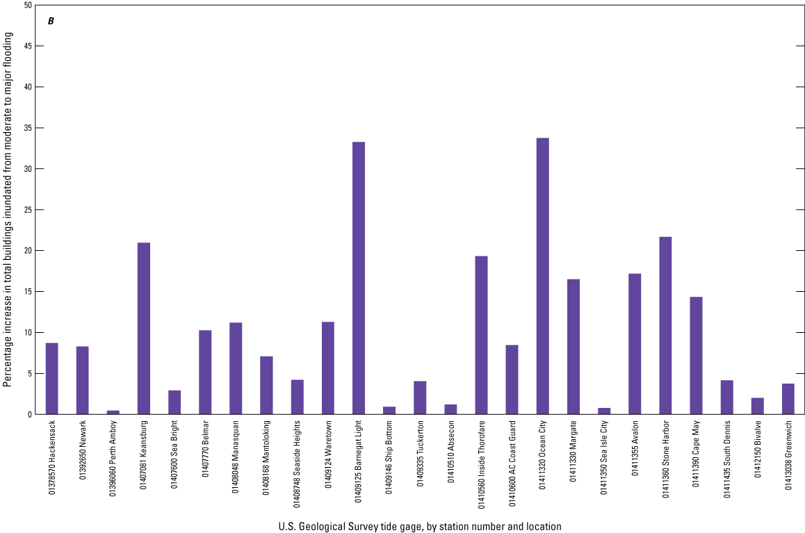
Graphs showing, A, the percent of major roads affected by flooding at moderate and major flood stage displayed by station extents, and, B, the percent increase in building structures inundated by station extents when flood stage was increased from moderate and major.
It is important to recognize evaluating impacts at moderate flood stage should include an understanding of potential escalation of impacts if the forecast or peak storm surge exceed moderate flood stage. This concept allows for anticipating uncertainty related to a storm forecast with the potential of disproportionate increases in damages beyond the threshold of a flood category like moderate flooding. For example, if the storm surge scenarios estimate a rapid expansion of damages or impacts beyond the limits, or edge, of moderate flooding it could be suggested that the range of moderate flooding is too broad. Emergency managers, responders, and the greater communities in general may benefit from a slightly reduced range to allow for a more proportional increase in damages. Analyzing the change in potential impacts between moderate and major flooding to evaluate if the edge of the thresholds allows for a somewhat gradual increase in damages as flood levels transition from moderate to major flooding was defined as an “edge analysis” for this study. The difference in elevation between the NWS moderate and major flood stages at most tide gages used in this study was generally about 1 ft. This was considered an acceptable increase for an edge analysis for these coastal areas due to the inherent uncertainty of hurricane and tropical storm force winds and associated storm surge. The mean increase in percent of building structures inundated per station extents was almost 12 percent with a few station extents showing increases of more than 20 to 30 percent (fig. 17B). The median increase was almost 8 percent reflecting that only a handful of communities within the station extents of the Keansburg, Barnegat Light, Ocean City, and Stone Harbor tide gages change substantially between moderate and major flooding. Notably, the communities of Sea Isle City and Ship Bottom demonstrate amongst the lowest percent increase, likely owing to the significant building inundation that is already occurring at moderate flooding. The mean increase in percent of buildings with 1 ft or more of inundation above the first-floor elevation was only 1 percent which may indicate as coastal flooding increased, the inundation spread outwards.
Many factors combine to influence general perception of coastal flood risk for different communities. Major hurricanes or coastal storms sometimes provide a perception of risk for several years, but it may diminish over time. The community understanding of coastal flood risk can also be influenced by several factors related to the most recent major storm track, distance of wind field from the community, and overall size and strength of the storm. To help strengthen resiliency and improve early warning impact mitigation plans, the combined vulnerability of building structures and transportation routes (major roads and bridges) to inundation from the simulated moderate flood scenarios was analyzed. Gaining a better understanding of the variability of flood impacts among coastal communities of New Jersey during moderate flooding (when it is perceived that significant impacts begin to occur) could provide valuable information about which communities may be at greater risk relative to the average of all communities in the study. Furthermore, use of a few common characteristics to experiment with methods to assign a mathematically computed score or moderate flood risk value for each mapped area was assumed. Using an equation to evaluate the variability of moderate flood risk helps reduce the subjectiveness of identifying one area as more vulnerable than another, and it provides a common means of calculating an estimated community risk.
The first method tested utilizes a few characteristics for building structures and transportation including percent of major roads inundated and number of major bridge crossings with disrupted access due to flooding. The resulting value was defined as the Coastal Community Moderate Flood Risk (CCMFR) score. Communities scoring a higher CCMFR score would be considered more vulnerable to coastal flood inundation. The primary categories tested were total buildings in the moderate flood area, percent of building structures with any level of inundation, building structures with greater than 1 ft of flooding above first-floor, building structures with greater than 3 ft of flooding above first-floor, percent of major roads inundated, and percentage of major bridges inundated or with inundated approaches rendering the bridge unusable. Using these categories, a weighting factor (defined as the ratio of the percent of community impact to the average of all communities) was applied to each category and the resulting value was computed for each mapped extents of moderate flooding.
whereRFB
is the ratio of community flooded buildings to average of all communities;
R1F
is the ratio of percent of building with flooding 1ft or more above first floor to the average percentage for all communities;
R3F
is the ratio of percent of building with flooding 3 ft or more above first floor to the average percentage for all communities; and
RMR
is the ratio of percent of major road inundated to average percent of major roads inundated for all communities.
The second method is similar to the first but uses two sets of fixed weighting factors for each characteristic. The selection of which weighting factors are used is done with a distribution factor (df). The z-score, also referred to as the standard score in statistics, was computed for total building structures inundated at moderate flooding and used to define df. The z-score is the measure of how many standard deviations the value is above or below the standard deviation of the dataset. For these equations, df was computed for moderate flooding using the percent of total building structures inundated in the local station extents to the average percentage of buildings inundated for all mapped station extents in the study. The value of df was computed for each storm scenario at all station extents and the two-storm average was used in the application of CCMFRweighted equation. Similar to the base CCMFR score, communities scoring a higher CCMFRweighted score would be considered more vulnerable to coastal flood inundation. Once computed, a positive value of df greater than 1 is used to apply more weight to percent of total structures inundated and percent with 1 ft or more of inundation and less on those with greater than 3 ft and total roads inundated. As noted earlier, building structures exposed to inundation are being used as a surrogate for people being directly impacted by flooding. It was assumed a community with a percentage of buildings, and therefore people, inundated beyond one standard deviation from the average should have a higher weight applied to total volume of exposure and slightly less on depth greater than 3 ft at the inundated structures. The value of df is used to select between the following equations providing the ability to adjust weighting for communities with total percent of buildings inundated positively skewed by more than one standard deviation at moderate flooding.
If the distribution factor (df) is greater than 1,
wherePFB
is percent of flooded building structures in moderate flood area;
P1F
is percent of building structures with 1 ft or more of inundation above first-floor elevation;
P3F
is percent of building structures with 3 ft or more of inundation above first-floor elevation; and
PMR
is percent of major roads flooded.
If df is less than 1,
The resulting experimental methods produced similar results partially because they apply similar importance to building structure inundation. The CCMFR scores ranged from very low (nearly zero) to a high of just over 50. Although a ratio and weighting method were both tested and additional weighting was applied for communities with higher-than-average building inundation, the results were generally similar. A threshold of twice the average for all communities was identified as an initial cutoff point used to select mapping extents that may be at higher risk for impacts from moderate flooding. Overall, five station extents exceeded this threshold although one of the five was just over the cutoff limit. Considering the four station extents that clearly exceeded the threshold, two of the four were identified by both equations. The station extents for the tide gages at East Thorofare at Ship Bottom (USGS station no. 01409146) and Beach Thorofare at Margate (USGS station no. 01411330) exceeded twice the average score for both experimental equations. The resulting CCMFR scores for each tide gage mapped area are shown in figure 18. This analysis tried to focus on evaluating the variability of flood impacts among areas within the mapped extents for each tide gage to help identify outliers or areas where increased flood risk education or mitigation efforts would have the highest cost to benefit ratio. Reducing subjective determinations of compounded coastal storm surge flood risk is a result of using measurable characteristics and developing mathematical equations. Future studies could improve this analysis by reviewing documented damages, and applying more characteristics, demographics, better categorization of transportation routes, and critical facilities to test and validate usefulness of the CCMFR value.
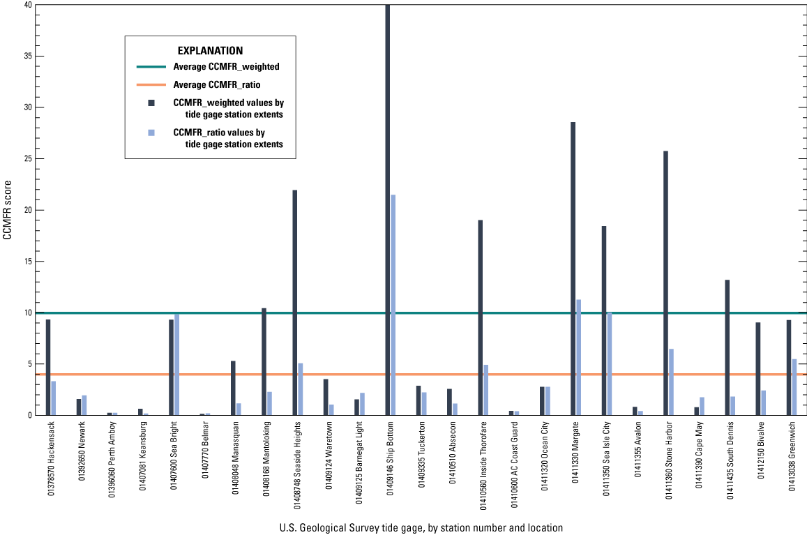
Graphs showing results of experiments Coastal Community Moderate Flood Risk (CCMFR) equation values for each of the 25 mapped station extents.
Evaluating National Weather Service Coastal Impact Statements
The NWS Philadelphia/Mount Holly forecast office created flood categories for many of the USGS tide gages used in this study. Often, NWS flood categories are determined through coordination between the NWS and local planning or emergency management officials. NWS impact statements typically accompany the categories and offer a general text description of the flooding conditions or areas being impacted by flooding. References to major roads or indications of flooding in select communities is often listed to give users information about the level of flood risk.
The inundation layer for the elevation closest to the NWS moderate flood stage was used to provide an evaluation of the impact statements (as of March 2022) listed within the NWS Advanced Hydrologic Prediction Service (AHPS) web page for each gage (National Oceanic and Atmospheric Administration, 2022a). Because the statements are created somewhat subjectively, the evaluation tried to include a few characteristics that were directly measurable to add a degree of uniformity to the analysis. The results of a combined visual review and comparison of percent of building structures inundated and major roads affected were used to identify outliers where further review by the NWS may be beneficial. As described earlier in this report, the average percentage of building structures within all mapped station extents indicated as being inundated by the simulated moderate flooding level was about 5 percent, but the range of structures inundated in some station extents varied from 10 to greater than 30 percent and was greater than 80 percent in two station extents (fig. 15). When the percentage of major roads affected by moderate flooding in these same mapped station extents were evaluated a few showed dramatically different results, although, several indicated a common theme when compared to building structure inundation. Seven station extents indicated 30 percent or more of total structures inundated at moderate flood stage and two of the seven also showed 20 percent or more of major roads inundated at moderate flood stage (fig. 17A). These metrics were used to help review and evaluate the existing NWS flood impact statements for the communities located within the 25 mapped station extents studied. A summary of the review and evaluation is provided in appendix 1.
Flood-Inundation Map Delivery
This study developed an online user interface to allow the coastal flood inundation maps for each of the 25 USGS tide gages to be seen by the public (https://webapps.usgs.gov/infrm/fdst/?region=nj). The inundation maps for the synthetic storm scenarios are linked to each of the tide gages in the study so users can easily navigate from the real-time data page to a visualization of inundation for communities adjacent to each gage. Figure 19 is a flow chart that describes one possible way the user could utilize real-time tidal elevation data from a USGS tide gage and the new NJWSC online coastal flood mapping tool to visualize the potential flooding from a storm event. The user would first get familiar with the USGS tide gage network, then identify a local landmark or reference to relate typical tidal elevations with the local landscape, then transition to the USGS NJWSC online coastal flood mapping tool. Once the user is in the mapping tool, they would navigate to their community or local coastal community of interest. Using the menus and selection options, the user can see the potential impacts from one of the two storm scenarios simulated for all locations in the study. The coastal inundation mapper allows the user to also select the level of inundation relative to the scale for tidal elevation on the real-time tide for their community. Utilizing the real-time tide gage network, the inundation scenarios illustrated in the coastal flood inundation mapping tool, and weather and storm forecasts, users can potentially better understand how the flooding spreads and plan for their own protection and that of their property. Figure 20 illustrates finding a tide gage, selecting a storm scenario, and selecting a flood inundation level. Not illustrated in figure 20 but available, is supplementary information, including historic peaks, a linked real-time hydrograph from the tide gage, and a link directing users to AHPS that provides forecasted tidal peaks for the gages located within the mapping tool. AHPS provides forecasts for tide gages in MLLW datum. To convert from MLLW to NAVD 88, users can follow the link on the AHPS web interface to the NOAA Tides and Currents webpage to obtain the appropriate conversion factor for the tide gage they are interested in. The coastal flood inundation maps can also be accessed directly by going to the USGS Flood Decision Support Tool webpage (https://webapps.usgs.gov/infrm/fdst/). The inundation grids, associated geospatial data, and supporting information for each flood inundation map library were also published and available in Niemoczynski and others (2023) and are available for public download.
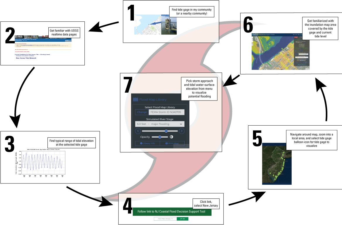
Flow chart showing an example of steps a user can follow to make a connection between U.S. Geological Survey (USGS) tide gage data and the New Jersey Water Science Center coastal flood inundation mapper.
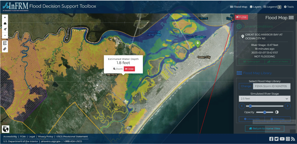
Example of an inundation map for a selected community, flood scenario, and inundation level generated by the New Jersey Water Science Center coastal flood inundation mapping tool.
Uncertainties and Limitations Regarding Use of Flood-Inundation Maps
Although the flood-inundation maps represent the boundaries of inundated areas with a distinct line, some uncertainty is associated with these maps. The flood boundaries shown were estimated based on interpolating measured water stage and simulated water-surface elevation derived from the output of a hydrodynamic model developed by FEMA Region II. Unique and somewhat unpredictable meteorological factors such as rapid changes in wind speed and direction associated with coastal storms and hurricanes can produce actual water-surface elevations and inundation boundaries that deviate from the inundation scenarios presented in this study. Additional uncertainties and limitations previously described, such as hydraulic connectivity and distance to the tide gage within an inundation map extent, may result in deviations from actual water-surface elevations during a coastal storm event. If this series of flood-inundation maps will be used in conjunction with NWS coastal forecasts, the user needs to be aware of additional uncertainties that may be inherent or factored into NWS forecast procedures (for more information, see http://water.weather.gov/ahps/pcpn_and_river_forecasting.pdf).
Summary
New Jersey has a dense coastal community with an approximate population of 5.6-million year-round residents. During the summer season the population dramatically increases which also coincides with the start of hurricane season for the eastern United States. Historically hurricanes and other coastal storms have created extensive damage for New Jersey’s coastal communities with storm surge inundation being the top risk factor. Hurricane Sandy devastated the coast of New Jersey in 2012, creating nearly $20 billion in building structure losses and stands as a major disaster benchmark. Many losses from coastal storms that occur more frequently and generate moderate to major flood stage conditions could be reduced with more education about the areas at highest risk for inundation. Although static flood hazard maps developed by the U.S. Army Corps of Engineers and the Federal Emergency Management Agency (FEMA) exist, they represent more extreme and catastrophic conditions caused by large hurricanes. Therefore, it is often difficult to communicate the risk of coastal flooding from more common storm events like those that generate inundation like the National Weather Service’s (NWS) moderate to major flood stages. Previous flood-inundation studies in the riverine environment have motivated residents, who otherwise might have ignored the warnings, to heed warnings and take action by providing a tool that shows the potential extent of flooding. (Niemoczynski and Watson, 2016). Developing a tool to depict storm surge flooding is more difficult because of the complex hydrodynamics that occur along the coast. Some communities have made efforts to utilize a simplified flat water-surface, or “bathtub,” approach to display coastal flooding but those methods do not display wind-driven storm surge conditions. The “bathtub” approach assumes a consistent rise in water-surface elevation across an estuary, tidal river, or tributary. This often does not adequately portray the effects of storm forces that can cause enhanced water-surface elevations in specific areas, resulting in a product that is inadequate at conveying flood risk.
This study utilized the output from the hydrodynamic model developed as part of the FEMA Region II Coastal Storm Surge Study. The model was a loose coupling of the ADvanced CIRCulation Model with the Simulating Waves Nearshore model. Utilizing the time series output of water-surface elevation from a hydrodynamic model and relating the simulated and measured water-surface elevation at each of the 25 U.S. Geological Survey (USGS) tide gage and map extents, allowed for the development of storm driven inundation maps linked to 25 USGS real-time tide gages along the coast of New Jersey. The resulting coastal flood inundation map libraries provide visualization of community flooding from tide elevations beginning at or near NWS flood stage and extending above NWS major flood stage. The USGS developed the Flood Decision Support Tool, which is a web mapping interface where users can interact with the map layers online and explore potential flooding for two coastal storm scenarios within specified areas surrounding the tide gages used in this study. The storm scenario inundation maps provide community officials and the public an opportunity to evaluate when buildings and streets may become flooded so they can plan response and mitigation actions to reduce damages. Visualizing when major roads become inundated during moderate flood conditions helps people realize the need to react to moderate flood warnings and plan for potential alternative transportation routes.
Beyond providing inundation maps to allow users to visualize inundation from coastal storms, this study evaluated the impact of moderate flooding on building structures and major roads for the mapped station extents at all 25 tide gages. The mean percentage of buildings in the moderate flood stage inundation area identified as potentially inundated was about 5 percent, but some mapped areas had building inundation percentages of greater than 20 to nearly 50 percent. Major roadways were also evaluated and indicated a mean percentage of almost 7 percent of all major roadways affected at moderate flood stage. This percentage increased to more than 11 percent at major flood stage. This information was used in combination with data about the percentage of buildings inundated above the first-floor elevation to develop some experimental methods for objectively evaluating community impact from coastal flooding. Two sets of equations defined as the coastal community moderate flood risk (CCMFR) score are being evaluated to see if they are effective at identifying communities at potentially higher risk from similar moderate flood conditions. The equations each potentially identified four to five mapped station extents that scored higher than twice the average for all communities but only two of the four mapped station extents were identified by both equations. More investigation is needed to add more information about critical facilities and demographics and cross reference public damage and claims records to better evaluate the performance of these equations. Overall, the New Jersey coastal flood maps, served on the USGS Interagency Flood Risk Management (InFRM) Flood Decision Support Toolbox (FDST) webpage, provide visualization capabilities for emergency management officials and the public to help all individuals better understand coastal flood risk in New Jersey.
References Cited
Danielson, J.J., Poppenga, S.K., Tyler, D.J., Palaseanu-Lovejoy, M., and Gesch, D.B., 2018, Coastal National Elevation Database: U.S. Geological Survey Fact Sheet 2018–3037, 2 p. [Also available at https://doi.org/10.3133/fs20183037.]
Esri, 2021, How topo to raster works: Esri web page, accessed November 5, 2021, at https://pro.arcgis.com/en/pro-app/2.8/tool-reference/3d-analyst/how-topo-to-raster-works.htm.
Federal Emergency Management Agency, 2016, Guidance for flood risk analysis and mapping—Statistical simulation methods: Department of Homeland Security, 32 p., accessed September 30, 2022, at https://www.fema.gov/sites/default/files/documents/fema_coastal-statistical-simulation-methods_nov-2016.pdf.
Federal Emergency Management Agency, 2021a, Zone V: Department of Homeland Security website, accessed November 5, 2021, at https://www.fema.gov/glossary/zone-v.
Federal Emergency Management Agency, 2021b, FEMA flood map service center—Welcome!: Department of Homeland Security website, accessed November 5, 2021, at https://msc.fema.gov/portal/home.
Federal Emergency Management Agency, 2022, Hazus: Department of Homeland Security web page, accessed July 27, 2022, at https://www.fema.gov/flood-maps/products-tools/hazus.
National Oceanic and Atmospheric Administration, 2022a, National Weather Service advanced hydrologic prediction service: Department of Commerce web page, accessed January 4, 2022, at https://water.weather.gov/ahps2/index.php?wfo=phi.
National Oceanic and Atmospheric Administration, 2022b, Tides & Currents Station 8531545, Keyport, Raritan Bay, NJ: Department of Commerce web page, accessed January 4, 2022, at https://water.weather.gov/ahps2/index.php?wfo=phi.
National Oceanic and Atmospheric Administration, 2022c, Vertical datum transformation—About VDatum: Department of Commerce web page, accessed January 4, 2022, at https://vdatum.noaa.gov/about.html.
National Weather Service, 2022a, Glossary—Flood stage: Department of Commerce web page, accessed January 5, 2022, at https://w1.weather.gov/glossary/index.php?word=flood+stage.
National Weather Service, 2022b, Glossary—Moderate flooding: Department of Commerce web page, accessed August 10, 2022, at https://w1.weather.gov/glossary/index.php?word=moderate+flooding.
National Weather Service, 2022c, Glossary—Major flooding: Department of Commerce web page, accessed August 10, 2022, at https://w1.weather.gov/glossary/index.php?word=major+flooding.
New Jersey Department of Environmental Protection and New Jersey Geological Survey, 2002, Physiographic provinces of New Jersey: Digital Geologic Series DGS02-7, accessed July 27, 2002, at https://www.state.nj.us/dep/njgs/geodata/dgs02-7.htm.
New Jersey Department of Transportation, 2021, GIS data—New Jersey Roadway Network: State of New Jersey website, accessed July 27, 2022, at https://nj.gov/transportation/refdata/gis/data.shtm/.
New Jersey Office of Geographic Information Systems, 2018, Parcels composite of New Jersey: New Jersey Department of Environmental Protection Bureau of GIS, accessed July 27, 2022, at https://www.arcgis.com/home/item.html?id=d543ddcc1e6844319ffa826fee52fccf.
New Jersey Office of Geographic Information Systems, 2022, Municipal boundaries of New Jersey: New Jersey Geographic Information Network website, accessed July 27, 2022, at https://njogis-newjersey.opendata.arcgis.com/datasets/newjersey::municipal-boundaries-of-nj/about.
New Jersey Sea Grant Consortium, 2022, Coastal concerns, National Oceanic and Atmospheric Administration web page, accessed January 3, 2022, at https://njseagrant.org/extension/coastal-concerns/.
Niemoczynski, L.M., Niemoczynski, M.J., Boetsma, A.C., and Suro, T.P., 2023, Synthetic storm-driven flood-inundation grids for coastal communities in 10 New Jersey counties. U.S. Geological Survey data release, at https://doi.org/10.5066/P9RVF9P8.
Niemoczynski, M.J., and Watson, K.M., 2016, Flood-inundation maps for the Peckman River in the townships of Verona, Cedar Grove, and Little Falls, and the Borough of Woodland Park, New Jersey, 2014: U.S. Geological Survey Scientific Investigations Report 2016–5105, 13 p. [Also available at https://doi.org/10.3133/sir20165105.]
Suro, T.P., Deetz, A., and Hearn, P., 2016, Documentation and hydrologic analysis of Hurricane Sandy in New Jersey, October 29–30, 2012: U.S. Geological Survey Scientific Investigations Report 2016–5085, 73 p., accessed December 17, 2021, at https://doi.org/10.3133/sir20165085.
The SWAN Team, 2022, The SWAN User Manual, SWAN Cycle III version 41.41, accessed January 18, 2022, at https://swanmodel.sourceforge.io/download/zip/swanuse.pdf.
U.S. Geological Survey, 2021, Flood inundation mapping program: U.S. Geological Survey Water Resources Science, accessed December 17, 2021, at http://www.usgs.gov/mission-areas/water-resources/science/flood-inundation-mapping-fim-program#overview.
U.S. Geological Survey, 2022a, Interagency flood risk management—Flood decision support toolbox: Department of the Interior, accessed January 4, 2022, at http://webapps.usgs.gov/infrm/fdst.
U.S. Geological Survey, 2022b, USGS water data for the nation: U.S. Geological Survey National Water Information System database, accessed January 4, 2022, at https://waterdata.usgs.gov/nj/nwis/current/?type=tide&group_key=basin_cd. [Also available at https://doi.org/10.5066/F7P55KJN.]
Appendix 1. Review of Major Communities and General Inundation Impacts to Building Structures Using Simulated Moderate Flood Area Extents and National Weather Service Moderate Flood Stage
[NWS, National Weather Service; MLLW, mean lower low water; NAVD 88, North American Vertical Datum of 1988; USGS, U.S. Geological Survey; N.J., New Jersey; —, no data; Rt, Route; Ave, Avenue; St, Street; Blvd, Boulevard; Dr, Drive; NA, not available; NC, no comments]
Conversion Factors
Datum
Vertical coordinate information is referenced to the North American Vertical Datum of 1988 (NAVD 88).
Horizontal coordinate information is referenced to the North American Datum of 1983 (NAD 83).
Abbreviations
ADCIRC
ADvanced CIRCulation Model
AHPS
Advance Hydrologic Prediction Service
BFE
Base Flood Elevation
CCMFR
Coastal Community Moderate Flood Risk
CoNED
Coastal National Elevation Database
CS
critical structure
df
distribution factor
FDST
Flood Decision Support Toolbox
FEMA
Federal Emergency Management Agency
FIRM
flood insurance rate map
FIS
flood insurance study
GIS
geographic information system
HAG
highest adjacent grade
InFRM
Interagency Flood Risk Management
JPM
Joint Probability Method
LAG
lowest adjacent grade
MLLW
mean lower low water
NAD 83
North American Datum of 1983
NAVD 88
North American Vertical Datum of 1988
NJDEP
New Jersey Department of Environmental Protection
NJDOT
New Jersey Department of Transportation
NJOEM
New Jersey Office of Emergency Management
NJTN
New Jersey Tide Network
NJWSC
New Jersey Water Science Center
NOAA
National Oceanic Atmospheric Administration
NWS
National Weather Service
NWIS
National Water Information System
PVSC
Passaic Valley Sewerage Commission
RAMPP
Risk Assessment, Mapping, and Planning Partners
SFHA
Special Flood Hazard Area
SMS
Surface-water Modeling System
SWAN
Simulating Waves Nearshore Model
TBDEM
topobathymetric digital elevation model
USGS
U.S. Geological Survey
USACE
U.S. Army Corps of Engineers
VDatum
Vertical Datum Transformation Utility
For more information, contact:
Director, New Jersey Water Science Center
3450 Princeton Pike Suite 110,
Lawrenceville, New Jersey 08648
Or go to our website at https://www.usgs.gov/centers/new-jersey-water-science-center.
Publishing support provided by the West Trenton Publishing Service Center.
Suggested Citation
Suro, T.P., Niemoczynski, M.J., Boetsma, A., and Niemoczynski, L.M., 2023, Moderate flood level scenarios—Synthetic storm-driven flood-inundation maps for coastal communities in 10 New Jersey counties: U.S. Geological Survey Scientific Investigations Report 2023–5005, 49 p., https://doi.org/10.3133/sir20235005.
ISSN: 2328-0328 (online)
Study Area
| Publication type | Report |
|---|---|
| Publication Subtype | USGS Numbered Series |
| Title | Moderate flood level scenarios—Synthetic storm-driven flood-inundation maps for coastal communities in 10 New Jersey counties |
| Series title | Scientific Investigations Report |
| Series number | 2023-5005 |
| DOI | 10.3133/sir20235005 |
| Year Published | 2023 |
| Language | English |
| Publisher | U.S. Geological Survey |
| Publisher location | Reston, VA |
| Contributing office(s) | New Jersey Water Science Center |
| Description | Report: viii, 49 p.; Data Release |
| Country | United State |
| State | New Jersey |
| County | Atlantic County, Bergen County, Cape May County, Cumberland County, Essex County, Middlesex County, Monmouth County, Ocean County, Salem County, Union County |
| Online Only (Y/N) | Y |
| Additional Online Files (Y/N) | N |
| Google Analytic Metrics | Metrics page |