

Development of an Integrated Hydrologic Flow Model of the Rio San Jose Basin and Surrounding Areas, New Mexico
Links
- Document: Report (5.62 MB pdf) , HTML , XML
- Plate: Plate 1 (550 KB pdf)
- Data Release: USGS data release—GSFLOW, used to run PRMS and MODFLOW-NWT models, to simulate the effects of natural and anthropogenic impacts on water resources in the Rio San Jose Basin and surrounding areas, New Mexico
- Download citation as: RIS | Dublin Core
Abstract
The Rio San Jose Integrated Hydrologic Model (RSJIHM) was developed to provide a tool for analyzing the hydrologic system response to historical water use and potential changes in water supplies and demands in the Rio San Jose Basin. The study area encompasses about 6,300 square miles in west-central New Mexico and includes the communities of Grants, Bluewater, and San Rafael and three Native American Tribal lands: the Acoma and Laguna Pueblos and the Navajo Nation. Perennial surface water features are sparse in the study area and most water resources consist of groundwater pumped from sedimentary and basalt aquifers.
Calibration of the RSJIHM was performed using PEST++ (version 4.3.20) and BeoPEST (version 13.6). Model parameter values were adjusted during calibration to fit model simulated values to the measured or estimated values for several observation groups: (1) solar radiation, (2) potential evapotranspiration, (3) actual evapotranspiration, (4) precipitation and minimum and maximum air temperature, (5) snow water equivalent, (6) snow-covered area, (7) streamflow, (8) hydraulic head, (9) springflow at Ojo del Gallo, (10) springflow at Horace Springs, (11) surface-water releases from Bluewater Lake, and (12) surface-water diversions for irrigation within the Bluewater-Toltec Irrigation District.
The simulated average annual hydrologic budget from 1950 through 2018 indicated that the majority (greater than 98 percent) of precipitation within the basin was consumed by evapotranspiration, leaving 1.2 percent to recharge the groundwater system, 0.47 percent to direct runoff to streams, and 0.20 percent to infiltrate the soil zone and interflow to streams. The average annual recharge to the groundwater system and runoff to streams simulated by the RSJIHM was about 28,000 and 11,000 acre-feet, respectively. The RSJIHM simulated about 590,000 acre-feet of cumulative aquifer storage depletion from 1950 through 2018.
Additional work that could improve the simulation capability of the RSJIHM includes (1) further data collection (streamflow, head, springflow) in the southwestern subbasin that includes the El Malpais National Monument, (2) incorporating temporally variable vegetation parameters, (3) spatial downscaling of the hydrometeorological input datasets, (4) incorporating additional spatial variability to hydraulic property parameters on the basis of new data collection, and (5) using environmental tracers to verify and calibrate model parameters.
Introduction
The Rio San Jose Integrated Hydrologic Model (RSJIHM) was developed to provide a tool for analyzing the hydrologic system response to historical water use and potential changes in water supplies and demands in the Rio San Jose Basin (defined in this report as the surface-water drainage basin; hereafter referred to as “the basin”) and surrounding areas (study area) in New Mexico (fig. 1; see “Description of Study Area” section). The study area includes the communities of Grants, Bluewater, and San Rafael and three Native American Tribal lands: the Acoma and Laguna Pueblos and the Navajo Nation. The water rights of the Pueblos of Acoma and Laguna are being adjudicated, along with other users in the basin, on the basis of past and present water use in the State of New Mexico, ex rel., State Engineer v. Kerr-McGee Corporation, and others (Utton Transboundary Resources Center, 2015). The RSJIHM is an integration of the U.S. Geological Survey (USGS) Precipitation-Runoff Modeling System (PRMS) (Markstrom and others, 2015) and MODFLOW-NWT (Niswonger and others, 2011) and provides a tool to help support long-term planning and management decisions regarding the basin’s surface-water and groundwater resources.
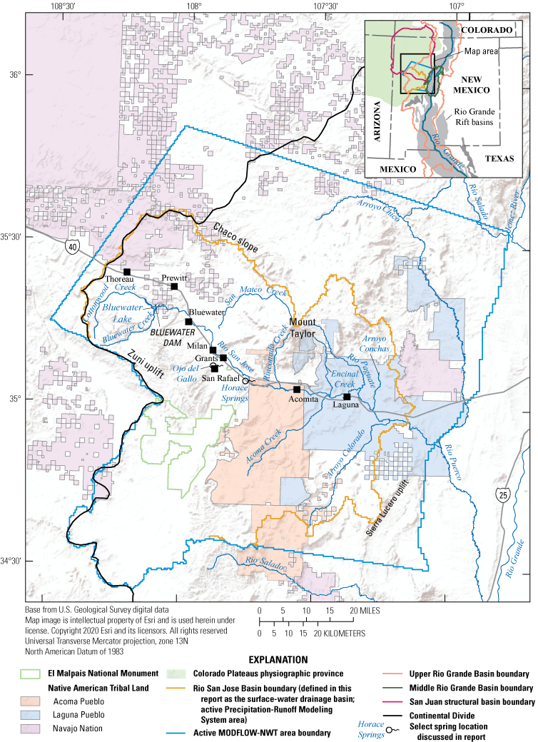
Study area and extent of the Rio San Jose Integrated Hydrologic Model in the Rio San Jose Basin and surrounding areas, New Mexico. Extent of Middle Rio Grande Basin modified from Plummer and others (2012). Extent of San Juan structural basin modified from Kernodle (1996). Extent of Rio Grande Rift modified from Hudson and Grauch (2013). Extent of Colorado Plateaus physiographic province from U.S. Geological Survey ([USGS], 2020). Extent of Upper Rio Grande Basin from Mankin and others (2022).
Purpose and Scope
The purpose of this report is to describe the construction, calibration, and assessment of the RSJIHM. This report describes the model boundaries, inputs, and parameterization, and summarizes the calibration results and model outputs including (1) hydrologic budgets and (2) calibrated hydraulic conductivity and storage properties. The performance of the RSJIHM is assessed by comparing model simulated values against measured, estimated, or reported values for (1) solar radiation, (2) potential evapotranspiration, (3) actual evapotranspiration, (4) precipitation and minimum and maximum air temperature, (5) hydraulic head, (6) streamflow, (7) springflow at Ojo del Gallo, (8) springflow at Horace Springs, (9) surface-water releases from Bluewater Lake, and (10) surface-water diversions for irrigation within the Bluewater-Toltec Irrigation District. Model performance also is evaluated in terms of mass balance errors and the conceptual understanding of the hydrologic system. Lastly, limitations and uncertainties of the model and suggestions for additional work are discussed.
Description of Study Area
The study area (active MODFLOW-NWT area) in west-central New Mexico encompasses about 6,300 square miles (mi2) and includes parts of three Native American Tribal lands: the Acoma and Laguna Pueblos and the Navajo Nation (fig. 1). The study area is situated in the Colorado Plateaus physiographic province and is bounded on the east by the tectonically active, north-south trending, half-graben, sedimentary basins of the Rio Grande Rift (fig. 1; Fenneman and Johnson, 1946; Murray and others, 2019). The study area is separated from the Middle Rio Grande Basin to the east by the Rio Puerco fault zone and Sierra Lucero uplift. The northern portion of the study area lies within the broad, gently northerly dipping Chaco slope subdivision of the San Juan structural basin and includes Mount Taylor, an extinct composite stratovolcano that reaches the highest elevations in the study area at greater than 11,000 feet (ft) (Kelley, 1950; Beaumont, 1987; Kernodle, 1996; Goff and others, 2013). The western boundary of the study area is roughly formed by the Continental Divide, which passes through the northwest-trending Zuni uplift (Kelley, 1950). The southwestern portion of the study area includes a closed surface-water drainage basin and upper Cenozoic basalt flows composing the El Malpais National Monument (Channer and others, 2015).
The Rio San Jose is the primary source of surface water in the basin. Originating in the Zuni uplift as Bluewater and Cottonwood Creeks, the Rio San Jose flows approximately 90 miles (mi) east-southeast from near the community of Bluewater to the Rio Puerco (fig. 1). Tributaries to the Rio San Jose include Cottonwood and Bluewater Creeks in the Zuni uplift, San Mateo Creek, Rinconada Creek, Acoma Creek, Encinal Creek, Rio Paguate, Arroyo Conchas, and Arroyo Colorado. Many of these streams are ephemeral at the confluence with the Rio San Jose; however, most are perennial in their upstream reaches (Risser and Lyford, 1983). Cottonwood and Bluewater Creeks flow to Bluewater Lake, which is a storage reservoir for agriculture and recreation in the area near the communities of Bluewater and Grants that was formed by the construction of Bluewater Dam in 1927 (Gordon, 1961).
Most of the rocks within the basin are sedimentary, except for Cenozoic basalts primarily associated with Mount Taylor and the basalt flows composing El Malpais National Monument, and Precambrian igneous and metamorphic rocks at depth and exposed in the Zuni uplift (Baldwin and Rankin, 1995; Sweetkind and others, 2020). Aquifers in the study area include, from youngest to oldest: (1) Quaternary alluvium and alluvial-basalt sequences; (2) Cenozoic basalts; (3) sandstones in the Cretaceous Mesaverde Group; (4) sandstone tongues in the Cretaceous Dakota Formation; (5) Jurassic rocks of the Jackpile Sandstone Member, the Brushy Basin Member, the Westwater Canyon Member, and the Recapture Member of Morrison Formation; (6) the Jurassic Bluff and Zuni Sandstone, the Todilto Limestone Member of Wanakah Formation of San Rafael Group, and the Entrada Sandstone of San Rafael Group; (7) sandstones in the Triassic Chinle Formation; and (8) the Permian San Andres Limestone and Glorieta Sandstone (Baldwin and Rankin, 1995). Older Permian (Yeso and Abo Formations) and Pennsylvanian (Madera Limestone) rocks are found at depths throughout most of the basin, except where exposed in the Zuni uplift and Sierra Lucero uplift, making groundwater withdrawals from these rocks prohibitively expensive and generally unnecessary because of the availability of groundwater from shallower rocks. Confining units within the stratigraphic sequence include the Cretaceous Mancos Shale deposits that underlie and intertongue with the Mesaverde Group and Dakota Formation, fine-grained deposits in the Brushy Basin Member of Morrison Formation, and fine-grained deposits in the Chinle Formation (Baldwin and Rankin, 1995).
Climate in the basin is semiarid to arid and is influenced by elevation and topography (Baldwin and Anderholm, 1992). A majority of the precipitation originates as convective storms during the summer monsoon in the lower elevations of the study area and as frontal winter storms in the higher elevations (Precipitation Runoff on Independent Slopes Model Climate Group, 2015; Western Regional Climate Center, 2020). Mean annual precipitation ranges from less than 10 inches (in.) at lower elevations in the basin to greater than 30 in. at higher elevations, and mean annual temperature varies from 56 degrees Fahrenheit (°F) at lower elevations to 38 °F at higher elevations (Precipitation Runoff on Independent Slopes Model Climate Group, 2015). Mean annual snowfall also varies greatly with elevation, ranging from less than 10 in. at lower elevations to greater than 50 in. at higher elevations in the Zuni uplift and Mount Taylor (Western Regional Climate Center, 2020).
History of Water Use
The basin has a long history of water use. Native Americans utilized surface-water resources in the basin for thousands of years prior to the arrival of non-Native settlers (Risser, 1982). Diversions of surface water for irrigation increased following the development of settlements in the area near the communities of Bluewater and Grants during the 1870s (Risser, 1982). Settlers began diverting springflow from Ojo del Gallo around 1870 (fig. 1), which had formerly discharged into a swampland and flowed into the Rio San Jose about 3 mi downstream from the community of Grants, to irrigate 1,000–2,000 acres of land in the area near the community of San Rafael (Risser, 1982; Frenzel, 1992). Ojo del Gallo springflow was utilized for irrigation of farms and gardens until the flow ceased in 1953 (Gordon, 1961). Prior to the construction of Bluewater Dam, settlers diverted surface water from Bluewater Creek for irrigation. Flows were regulated on Bluewater Creek from 1894 to 1909 when a series of earth dams were built near the current location of Bluewater Dam. Following the construction of Bluewater Dam in 1927, four main canals were constructed to deliver water diverted from Bluewater Creek to over 10,000 acres of land within the Bluewater-Toltec Irrigation District (Gordon, 1961). However, runoff to Bluewater Lake proved to be inconsistent from year to year and never large enough to support the intended acreage. By 1948 the amount of land within the Bluewater-Toltec Irrigation District had been permanently reduced to 5,488 acres (Gordon, 1961).
The inconsistency of interannual surface-water supply resulted in the introduction of large-capacity irrigation wells in 1944 and the rapid expansion of the number of wells during the 1940s (Risser, 1982). Most of these wells obtained water from the Permian San Andres Limestone and Glorieta Sandstone aquifer system (SAGA) (Gordon, 1961). On the Acoma and Laguna Pueblos, irrigation wells obtain water primarily from the Quaternary alluvium and alluvial-basalt sequences aquifer (Risser and Lyford, 1983).
Following the discovery of uranium in the basin in the early 1950s, the economy and resultant groundwater use began to shift from predominantly agricultural to industrial (Gordon, 1961; Risser, 1982). From 1951 to 1980, the Grants uranium district yielded more uranium than any other district in the United States (McLemore, 2011). Most of the uranium production was from the Westwater Canyon Member of Morrison Formation (McLemore, 2011), which at many mines required the dewatering of the ore-bearing and overlying units to access the ore. Numerous mills were constructed to process uranium, which also required large-capacity wells that pumped groundwater from the SAGA (Gordon, 1961). Untreated mine dewatering and mill-process waters were discharged to natural waterways and were a significant source of contamination of sediments, alluvial aquifers, and deeper aquifers in areas of faulting (Schoeppner, 2008). A variety of factors led to the cessation of mining activities in the 1980s (McLemore, 2011). Many springs ceased to flow during the mining period, and partial recovery of some springs was observed after mining operations ceased (Lorenzo and Watchempino, 2003).
Municipal development and water use expanded in the 1950s to meet the demands of the mining industry (Gordon, 1961; Frenzel, 1992). The population of the community of Grants grew from 2,251 in 1950 to 10,274 in 1960 (U.S. Census Bureau, 1960). The municipal water supply for the community of Grants was primarily obtained from the Quaternary alluvium and alluvial-basalt sequences aquifer prior to 1958 and from the SAGA afterward (Gordon, 1961; Cooper and West, 1967). Smaller communities around the community of Grants typically obtain municipal water supply from the SAGA and the Quaternary alluvium and alluvial-basalt sequences aquifer (Gordon, 1961; Cooper and West, 1967). Municipal water supply on the Acoma and Laguna Pueblos is obtained from a variety of aquifers, including the Quaternary alluvium, Dakota Formation, Zuni Sandstone, Entrada Sandstone, and sandstones in the Chinle Formation (Risser and Lyford, 1983).
Water for domestic and livestock use in the basin is obtained from springs and wells (Gordon, 1961). These domestic and livestock springs and wells obtain water from nearly all of the aquifers in the basin, but most wells obtain water from the SAGA or the Quaternary alluvium and alluvial-basalt sequences aquifer (Gordon, 1961). Many springs utilized for domestic and livestock use issue from the Cenozoic basalts aquifer on mesas near the community of Grants and Mount Taylor and in the Zuni uplift (Gordon, 1961; Risser and Lyford, 1983).
Previous Model Studies
Frenzel (1992) developed one of the first published hydrologic models within the basin and simulated groundwater flow, streamflow, and springflow using the MODFLOW-88 numerical code (McDonald and Harbaugh, 1988) with modifications. Groundwater flow was simulated in the Quaternary alluvium and alluvial-basalt sequences, Quaternary basalt aquifers, and the Permian SAGA. Streamflow was simulated in the Rio San Jose, in Bluewater and Cottonwood Creeks, and from Bluewater Lake. Springflow was simulated at Ojo del Gallo and Horace Springs (fig. 1). The three-dimensional model was calibrated to observations of groundwater levels and streamflows for a historical simulation period of fall 1899 to fall 1985. The calibrated model was then used to simulate scenarios of future groundwater development for a 35-year period. The scenario simulations indicated that 10,000 acre-feet (acre-ft) per year of groundwater withdrawal from the SAGA near the west side of the Acoma Pueblo resulted in groundwater-level declines but did not result in significant depletion of streamflows or springflow.
Daniel B. Stephens & Associates, Inc. (2001) updated the Frenzel (1992) model by extending the historical simulation time period through 1999, incorporating new information on groundwater withdrawals, and including new time-varying inputs of recharge, streamflow, and springflow for the extended simulation time period. Daniel B. Stephens & Associates, Inc. (2001) performed scenario simulations over a 50-year future period with and without additional groundwater withdrawal from the SAGA at the maximum water right (3,859 acre-feet per year [acre-ft/yr]) for selected wells under a range of climatic conditions (minimum, average, and maximum historical precipitation). The worst-case scenario (minimum precipitation and additional groundwater withdrawal from the SAGA at the maximum water right for selected wells) indicated that up to 115 ft of groundwater-level declines were possible, with depletion of streamflow in the Rio San Jose not likely to exceed 1 cubic foot per second (ft3/s) and more rapid drying of Ojo del Gallo springflow.
Hydrologic models have also been developed that focused on the hydrology in the vicinity of the Acoma and Laguna Pueblos. Risser and Lyford (1983) developed a two-dimensional, one-layer model of the Quaternary alluvium and alluvial-basalt sequences aquifer along the Rio San Jose from about 2 mi west of the boundary between the Acoma and Laguna Pueblos to the community of Laguna (fig. 1). The model was developed using the numerical code of Trescott and others (1976) and calibrated to observations of groundwater levels for a steady-state simulation period prior to 1976. The calibrated model was used to simulate several scenarios of groundwater withdrawals for future time intervals and indicated that the withdrawals generally resulted in depletions of aquifer storage, streamflows, and evapotranspiration. More recently, Ward (2017) developed a one-layer model that generally covered the same aquifer of Risser and Lyford (1983) and extended the modeled area further east to near the confluence of Arroyo Conchas with the Rio San Jose (fig. 1). Ward (2017) used the MODFLOW-2000 numerical code (Hill and others, 2000) and calibrated the model to observations of groundwater levels for a steady-state simulation period prior to 1973 and to observations of streamflow for a transient simulation period from 1973 through 2016.
Hydrologic models of the San Juan structural basin (fig. 1) have been developed by Frenzel and Lyford (1982), Kernodle (1996), and INTERA, Inc. (2012). Frenzel and Lyford (1982) developed a three-dimensional, seven-layer, steady-state model of the Cretaceous and Jurassic aquifers and confining units. The model was developed using the numerical code of Posson and others (1980) and calibrated to observations of groundwater levels and groundwater-level differences between aquifers. Frenzel and Lyford (1982) found that the vertical hydraulic conductivity of major confining-bed sequences ranged from 8.6×10−08 to 8.6×10−05 feet per day [ft/d] and that the ratio of horizontal hydraulic conductivity in aquifers to vertical hydraulic conductivity in confining-bed sequences generally ranged from 10,000 to 1,000,000. Kernodle (1996) developed a three-dimensional, 12-layer, steady-state model of the Cenozoic through Jurassic aquifers and confining units using the MODFLOW-88 numerical code (McDonald and Harbaugh, 1988). Similar to Frenzel and Lyford (1982), Kernodle (1996) defined the base of the model as the confining Chinle Formation and calibrated the model to observations of groundwater levels. Kernodle (1996) found that horizontal hydraulic conductivity of aquifers and confining units ranged from 0.1 to 1 ft/d and 5×10−05 to 5×10−02 ft/d, respectively, and vertical hydraulic conductivity was generally one to three orders of magnitude less than horizontal hydraulic conductivity. INTERA, Inc. (2012) developed a three-dimensional, 10-layer model similar in horizontal extent to the models of Frenzel and Lyford (1982) and Kernodle (1996) using the MODFLOW-SURFACT numerical code (HydroGeoLogic, Inc., 1996). INTERA, Inc. (2012) included units in the model from the land surface to the bottom of the Westwater Canyon Member of the Morrison Formation. The INTERA, Inc. (2012) model was calibrated to observations of groundwater levels for a steady-state simulation period prior to 1930 and to observations of groundwater levels and reported dewatering rates and total volume of groundwater withdrawn in uranium mining areas for a transient simulation period from 1930 through 2012. INTERA, Inc. (2012) used the model for scenario simulations over a 113-year future period to investigate the potential hydrologic impacts with and without dewatering at the proposed Roca Honda uranium mine to be located in the southeast part of the Ambrosia Lake subdistrict. INTERA, Inc. (2012) found that the proposed Roca Honda uranium mine dewatering would not adversely affect the water resources of the communities near the mine and would not have any adverse impacts on area springs.
Chavarria and others (2020) developed, calibrated, and assessed a hydrologic model of the Upper Rio Grande Basin, which generally included the Rio Grande Rift basins from the headwaters of the Rio Grande in Colorado to Texas (fig. 1), using PRMS (Markstrom and others, 2015). The PRMS model simulated natural streamflow conditions (streamflow that would occur in the absence of anthropogenic modifications) for the period 1980 through 2015 and included the Rio San Jose Basin. Chavarria and others (2020) found that as the Rio Grande flows southward, the compounding effects of both natural and anthropogenic influence on streamflow were evident with median measured streamflow 95 percent less than simulated near-native streamflow at the terminus of the Upper Rio Grande Basin for the period of simulation.
Modeling Approach and Construction
The USGS PRMS (version 5.2.0) and MODFLOW-NWT (version 1.2.0) were used to simulate the effects of natural and anthropogenic impacts on water resources in the study area (Ritchie and others, 2023). PRMS and MODFLOW-NWT were run uncoupled using the GSFLOW executable (version 2.2.0) (Markstrom and others, 2008). The GSFLOW executable also provides the option to run a coupled hydrologic model that integrates PRMS and MODFLOW-NWT at a daily time step (Markstrom and others, 2008; Regan and Niswonger, 2021), but this feature was not utilized in this study because of long run times and numerical instabilities. PRMS is a deterministic, process-based, distributed-parameter modeling system designed to analyze the effects of precipitation, climate, and land use on streamflow and general basin hydrology (Markstrom and others, 2015). MODFLOW-NWT is a Newton-Raphson formulation for the fifth core version of MODFLOW, MODFLOW-2005 (Harbaugh, 2005), that provides an improved numerical solution of models that simulate unconfined groundwater-flow systems (Niswonger and others, 2011). MODFLOW-NWT was used for this study to better represent the unconfined aquifers in the basin. The RSJIHM was developed by running PRMS and MODFLOW-NWT sequentially, with PRMS-simulated outputs (recharge, surface runoff to streams, and interflow from the soil zone to streams) fed into MODFLOW-NWT as inputs. Calibration of the RSJIHM also was performed sequentially, with PRMS calibrated first and MODFLOW-NWT with inputs derived from PRMS calibrated second.
Temporal Discretization
The transient simulation period for the RSJIHM extends from January 1, 1950, through September 30, 2018. The year 1950 was chosen as the first year of the simulation because of the availability of gridded daily climate datasets (precipitation, and minimum and maximum air temperature) needed to run PRMS (see “Climate Distribution Parameterization” section). The period from 1944 through 1949 was chosen to simulate steady-state conditions (hydraulic head [the elevation to which groundwater will rise in a tightly cased well; hereafter referred to as “head”] does not vary with time) and provide initial heads for the transient MODFLOW-NWT. The widespread development of groundwater resources in the basin began in 1944 and the impact of this development was incorporated in the steady-state simulation period by specifying an average annual groundwater withdrawal based on data from 1944 through 1949 (Gordon, 1961; Risser, 1982; data are available on request from the New Mexico Office of the State Engineer [NMOSE]). Because of the groundwater withdrawals, the steady-state simulation period does not represent steady-state conditions and large aquifer storage depletions are likely during the first couple of years of the transient simulation period as MODFLOW-NWT responds to the initial heads. PRMS was run on a daily time step, which corresponds to the smallest increment of time between consecutive measured input data values, such as precipitation and temperature (Markstrom and others, 2008). MODFLOW-NWT was discretized into 825 monthly stress periods with 1,650 equal-interval semimonthly time steps. In MODFLOW-NWT, stress periods correspond to changes in the specified boundary conditions, such as groundwater pumping, whereas time steps divide the stress period into finer increments that may be needed for numerical solution convergence or to improve the accuracy of the solution (Niswonger and others, 2011).
Precipitation-Runoff Modeling System
PRMS is designed to analyze the effects of precipitation, climate, and land use on streamflow and general basin hydrology on a daily time step (Markstrom and others, 2015). The input data used to construct the PRMS portion of the RSJIHM include a digital elevation model (DEM) to delineate the stream network, land and vegetation cover and soil datasets to generate land surface and soil zone parameters, and gridded daily climate datasets. Solar radiation, potential and actual evaporation, precipitation, air temperature, snow water equivalent, snow-covered area, and streamflow records were used to calibrate PRMS. The PRMS-simulated outputs compiled and used as inputs to MODFLOW-NWT were recharge, surface runoff to streams, and interflow from the soil zone to streams.
The active PRMS area for the RSJIHM is delineated into 15 subbasins using 12 streamgage locations, 2 closed surface-water subbasins, and the basin outlet (fig. 2). The active PRMS area is further partitioned into gridded hydrologic response units (HRUs), which are areas with relatively uniform hydrologic response that are based on watershed topography, vegetation, soil, and climate. Each HRU can be designated as one of four types: land, lake, swale, or inactive. The land-type HRU is the most common and simulates all the hydrologic processes in PRMS. The lake-type HRU is simulated with different algorithms that are applicable for the hydrologic properties of lakes. The swale-type HRU is a land-type HRU without the surface runoff and interflow components of lateral flow, which is suitable for simulating low areas that capture flow and only contribute to groundwater flow. The inactive-type HRU is excluded from the model simulation.
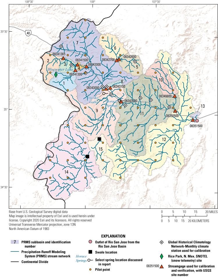
Precipitation-Runoff Modeling System (PRMS) stream network and subbasins, and the locations of climate stations where measured precipitation, minimum air temperature, and maximum air temperature were used for calibration of the Rio San Jose Integrated Hydrologic Model (RSJIHM), the Rice Park, New Mexico SNOTEL site where measured snow water equivalent was used for calibration of the RSJIHM, streamgages where measured streamflow was used for calibration and verification of the RSJIHM, pilot points where spatially variable PRMS parameters were adjusted during calibration of the RSJIHM, swales, and the outlet where the Rio San Jose exits the Rio San Jose Basin, New Mexico.
The GSFLOW-Arcpy toolkit was used to generate parameters needed to run PRMS (Gardner and others, 2018). The toolkit uses publicly available geospatial data to produce most parameters needed to run PRMS with gridded constant-area-square HRUs and some MODFLOW-NWT parameters. An in-depth explanation of the scripts and data development process is provided in Gardner and others (2018). The data and steps taken to generate the information needed to run PRMS, include the following:
-
Model boundary delineation and horizontal discretization.
-
Stream network delineation and streamflow routing.
-
Land surface and soil zone parameterization.
-
Climate distribution parameterization.
-
Snow-covered area parameterization.
-
Water use estimation and distribution.
Model Boundary Delineation and Horizontal Discretization
The active PRMS area conforms to the basin, encompassing a total area of about 3,600 mi2 (fig. 1) that was discretized into 500- by 500-meter (m) grid cells, each representing an HRU. The land surface elevation of each HRU was derived from a National Elevation Dataset 10-m horizontal resolution DEM (USGS, 2017) at the center of each grid cell. A total of 36,774 HRUs were active in PRMS, with 13 HRUs set as lake type to simulate Bluewater Lake, 2 HRUs set as swale type to simulate closed surface-water subbasins, and the remaining HRUs set as land type. The two swale HRUs were defined as the lowest DEM-derived land surface elevation within two closed subbasins (subbasins 14 and 15 in fig. 2) identified from National Hydrography Dataset (NHD) Hydrologic Unit Code 12 (USGS, 2019a) in the southwestern part of the study area.
Stream Network Delineation and Streamflow Routing
The HRU land surface elevations were used by the GSFLOW-Arcpy toolkit to develop the stream network, which includes the main-stem Rio San Jose and its major tributaries, and delineate subbasins in the active PRMS area (fig. 2). The level of detail of the stream network (density of tributaries to the Rio San Jose) was adjusted with the user defined values for flow accumulation and flow length thresholds until a level of detail that represented the Rio San Jose and its major tributaries was obtained. The stream network was modified to better match the location of NHD flow lines (USGS, 2019a) and stream networks visible in aerial imagery by manually adjusting select HRU land surface elevations. Fifteen subbasins were delineated using the 12 streamgages that were used for model calibration and verification (see “Precipitation-Runoff Modeling System, Calibration Approach and Datasets” section), the 2 swale HRUs (low areas that capture flow and only contribute to groundwater flow), and 1 outlet location where the Rio San Jose exits the basin.
Local depressions in the HRU land surface elevations that were not identified as swales were filled by the GSFLOW-Arcpy toolkit using the Cascade Routing Tool (version 1.3.1) (Henson and others, 2013). These local depressions (or undeclared swales) were filled, because they become HRUs with no downslope flow path and can cause numerical issues if a swale is not physically present (Henson and others, 2013). After the adjustments to the HRU land surface elevations, the toolkit used the Cascade Routing Tool with the stream network to compute the surface and shallow subsurface lateral flow paths (called cascades) among HRUs. The Cascade Routing Tool was also used to develop the associated cascade parameters required by PRMS to route simulated flows from upslope HRUs to downslope HRUs and cascade-discharge features such as streams, swales, or lakes. This study used the srunoff_smidx module to control surface runoff processes and the muskingum_lake module to control streamflow routing (Markstrom and others, 2015; Regan and LaFontaine, 2017).
Thirteen lake-type HRUs were used to simulate Bluewater Lake. The lake-type HRUs representing Bluewater Lake were defined as the grid cells with at least 30 percent of the cell area containing the NHD waterbody feature (USGS, 2019a). Managed releases from Bluewater Lake have altered the natural hydrologic system that is simulated by PRMS. Therefore, releases from Bluewater Lake were simulated in PRMS using the muskingum_lake module, with the outflow from Bluewater Lake specified in the PRMS data file. This flow replacement method does not maintain a complete water balance because the state (calculated water-content storage) of the lake is computed but not included in the water balance (Regan and LaFontaine, 2017).
Daily releases from Bluewater Lake were estimated for the transient simulation period without gaged flows using measured daily mean streamflow obtained from the USGS National Water Information System (NWIS) (USGS, 2019b) at the Bluewater Creek below Bluewater Dam, N. Mex. streamgage (referred to hereafter as “Bluewater Creek below Bluewater Dam”; USGS site number 08341500), which is about 2 mi downstream from Bluewater Dam. Using the streamflow at this streamgage to estimate releases from Bluewater Lake relied on the assumption that streamflow gains from groundwater and streamflow losses to groundwater were negligible between Bluewater Dam and the streamgage, which was reasonable because of the proximity of the streamgage to Bluewater Dam. Measured streamflow was available at the Bluewater Creek below Bluewater Dam streamgage for only a portion (March 17, 1951, through September 29, 1963, and July 21, 1989, through February 22, 2001) of the transient simulation period of the RSJIHM. Therefore, streamflow at the Bluewater Creek below Bluewater Dam streamgage needed to be estimated during the intervening transient simulation periods of the RSJIHM not covered by the measured streamflow data. About 8 mi downstream from Bluewater Dam is the Bluewater Creek near Bluewater, N. Mex. streamgage (referred to hereafter as “Bluewater Creek near Bluewater”; USGS site number 08342000). Measured daily mean streamflow obtained from the USGS NWIS (USGS, 2019b) was available for the Bluewater Creek near Bluewater streamgage from October 1, 1960, through January 4, 1973. Because of its proximity to Bluewater Dam, the Bluewater Creek below Bluewater Dam streamgage is likely most representative of releases from Bluewater Lake, but the Bluewater Creek near Bluewater streamgage provides an additional period (September 30, 1963, through January 4, 1973) of measured streamflow that was used to estimate streamflow at the Bluewater Creek below Bluewater Dam streamgage during this period.
The Bluewater Creek below Bluewater Dam and Bluewater Creek near Bluewater streamgages had an overlapping period of streamflow measurements from October 1, 1960, through September 29, 1963. Linear regressions (fig. 3) were developed for streamflow measurements at Bluewater Creek below Bluewater Dam versus two groups of streamflow measurements (daily mean streamflow less than or equal to 6 ft3/s and greater than 6 ft3/s) at Bluewater Creek near Bluewater during the overlapping period. To check the ability of these linear regressions to predict daily mean streamflow at Bluewater Creek below Bluewater Dam, the regressions were used to estimate daily mean streamflow at Bluewater Creek below Bluewater Dam from the daily mean streamflow at Bluewater Creek near Bluewater during the overlapping period. The estimated daily mean streamflow closely matched the measured daily mean streamflow at Bluewater Creek below Bluewater Dam, with a sum of daily differences (estimated minus measured) of 5 ft3/s and a root-mean-square error (RMSE) of daily differences of about 1 ft3/s, calculated as
wherei
is the ith pair of estimated or simulated and measured value,
S
is the estimated or simulated value associated with the ith measured value,
M
is the ith measured value, and
N
is the total number of pairs of estimated or simulated and measured values.
Therefore, the linear regressions were deemed suitable to estimate daily mean streamflow at Bluewater Creek below Bluewater Dam during the period from September 30, 1963, through January 4, 1973, when measured daily mean streamflow was only available at Bluewater Creek near Bluewater. The linear regressions had nonzero vertical axis intercepts (estimated daily mean streamflow at Bluewater Creek below Bluewater Dam), and therefore negative values of estimated daily mean streamflow at Bluewater Creek below Bluewater Dam were set to 0 ft3/s.
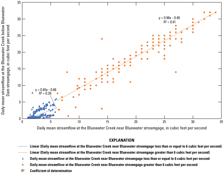
Linear regressions for streamflow measurements at the Bluewater Creek below Bluewater Dam, N. Mex. streamgage (U.S. Geological Survey site number 08341500) versus two groups of streamflow measurements (daily mean streamflow less than or equal to 6 cubic feet per second [ft3/s] and greater than 6 ft3/s) at the Bluewater Creek near Bluewater, N. Mex. streamgage (U.S. Geological Survey site number 08342000) during the overlapping period of streamflow measurements that were developed to estimate daily releases from Bluewater Lake for the transient MODFLOW-NWT.
During periods when measured daily mean streamflow was not available at either Bluewater Creek below Bluewater Dam or Bluewater Creek near Bluewater, daily mean streamflow was estimated using the annual mean streamflows (each being the arithmetic mean of the daily mean streamflow derived from Bluewater Creek below Bluewater Dam and Bluewater Creek near Bluewater, as described previously, for each year) and annual estimates of surface-water diversions for irrigation within the Bluewater-Toltec Irrigation District (data are available on request from the NMOSE). When annual surface-water diversions were estimated to be zero, daily mean streamflow was held constant during the year at 0.21 ft3/s (computed as the arithmetic mean of the annual mean streamflows for years with no surface-water diversions). When annual surface-water diversions were estimated to be greater than zero, daily mean streamflow was specified for growing season (28 ft3/s) and nongrowing season (2.6 ft3/s) periods (computed as the arithmetic mean of the annual mean streamflows for growing and nongrowing season subdivisions of each year). The growing and nongrowing season subdivisions of each year were estimated at a monthly frequency, with the growing season corresponding to months with a daily minimum air temperature greater than 32 °F for at least two-thirds of the month and the nongrowing season corresponding to the other months that did not meet these criteria. The daily minimum air temperature was obtained from the gridded, hydrometeorological datasets described in the “Climate Distribution Parameterization” section and analyzed for the growing and nongrowing season criteria at the HRU where surface water was diverted from Bluewater Creek below Bluewater Dam for irrigation within the Bluewater-Toltec Irrigation District.
Land Surface and Soil Zone Parameterization
Publicly available geospatial datasets along with the GSFLOW-Arcpy toolkit were used to produce spatially distributed land surface and soil zone parameters needed to run PRMS. The National Land Cover Dataset 2011 (USGS, 2014) was used to derive initial values for the fraction of each HRU area that is impervious (hru_percent_imperv), which were later adjusted during calibration (see “Precipitation-Runoff Modeling System, Calibration Approach and Datasets” section). Calibration of hru_percent_imperv was necessary, because the toolkit generated hru_percent_imperv values generally contradicted the classifications in the National Land Cover Dataset. For example, areas of the National Land Cover Dataset classified as “Developed, Low Intensity” to “Developed, High Intensity” (representing urban areas) had the lowest hru_percent_imperv values while areas of the National Land Cover Dataset classified as “Herbaceous” to “Shrub/Scrub” had the highest hru_percent_imperv values. The LANDFIRE 2014 (lf_1.4.0) Existing Vegetation Cover (Wildland Fire Science, Earth Resources Observation and Science Center, USGS, 2016a) and Existing Vegetation Type (Wildland Fire Science, Earth Resources Observation and Science Center, USGS, 2016b) datasets were used to generate parameters related to vegetation. The cov_type parameter defines the dominant vegetation type for each HRU (0=bare soil, 1=grasses, 2=shrubs, 3=trees, 4=coniferous), and with each vegetation type, an associated rooting depth is assigned. In addition, the summer vegetation cover density and winter vegetation cover density (covden_sum and covden_win) and summer rain interception storage capacity and winter rain interception storage capacity (srain_intcp and wrain_intcp) are determined from the vegetation type assigned to each HRU. The summer rain interception storage capacity (srain_intcp) derived from the GSFLOW-Arcpy toolkit was later adjusted during calibration (see “Precipitation-Runoff Modeling System, Calibration Approach and Datasets” section).
Soil zone parameters were derived from soils data obtained from the Digital General Soil Map of the United States or STATSGO2 (U.S. Department of Agriculture, Natural Resources Conservation Service, 2006). A dominant soil type (soil_type parameter; 1=sand, 2=loam, 3=clay), soil depth, and parameters influencing water movement through the soil were derived from the soils data. Soil depth is defined by the greater of the soil depth values provided by the soils data or rooting depth (Gardner and others, 2018). The maximum water holding capacity of the soil is determined by the parameter soil_moist_max, which influences processes such as evapotranspiration, surface runoff, and recharge (Markstrom and others, 2015). Parameters ssr2gw_rate and slowcoef_lin route water to the groundwater reservoir or to downslope HRUs (Markstrom and others, 2015).
Climate Distribution Parameterization
The Climate-by-HRU Distribution Module, climate_hru, was used to input daily precipitation and minimum and maximum air temperature by HRU to PRMS (Markstrom and others, 2015). This study assigned daily precipitation and minimum and maximum air temperature to each HRU by extracting data from gridded, hydrometeorological datasets (Livneh and others, 2015; Thornton and others, 2016) at the centroid of each HRU. The Livneh and others (2015) dataset was gridded at 1/16-degree horizontal resolution (approximately 6 kilometers [km]) and covered the period from 1950 through 2013. The Thornton and others (2016) dataset, known as Daymet, was gridded at a 1-km horizontal resolution and covered the period from 1980 through 2019. This study used the Livneh and others (2015) dataset for the RSJIHM transient simulation period from 1950 through 2013 and the Daymet dataset for the RSJIHM transient simulation period from 2014 through September 30, 2018. This study used the ddsolrad module to control the distribution of solar radiation to each HRU, the transp_tindex module to determine whether the dominant vegetation in each HRU is actively transpiring, and the potet_jh module to calculate the amount of potential evapotranspiration in an HRU.
Snow-Covered Area Parameterization
This study assigned snow area depletion curve values (snarea_curve parameter) and the maximum threshold snowpack water equivalent below which the snow-covered-area curve is applied (snarea_thresh parameter) to each HRU by extracting data from the USGS National Hydrologic Model (Regan and others, 2018) HRU occupying the majority of each RSJIHM HRU. In total, values for 184 snow area depletion curves from the USGS National Hydrologic Model were assigned to HRUs in the RSJIHM. Related parameters that were modified to accommodate these edits include ndepl (the number of snow-depletion curves), ndeplval (the number of values in all snow-depletion curves, equal to ndepl times 11), and hru_deplcrv (the index number for the snowpack areal depletion curve associated with each HRU).
Water Use Estimation and Distribution
Surface-water use in the basin has been primarily for irrigation and has varied in quantity throughout the simulation periods of the RSJIHM (Risser, 1982). Diversions of surface water from Bluewater Creek below Bluewater Dam for irrigation within the Bluewater-Toltec Irrigation District were simulated in PRMS using the water_use_read module as an external transfer of water from the stream network outside the active PRMS area (dest_type variable equal to 4) (Regan and LaFontaine, 2017). Water applied to the land surface for irrigation from those same diversions was simulated to infiltrate below the soil zone to recharge the groundwater system (hereafter referred to as “deep percolation”) in MODFLOW-NWT (see “MODFLOW-NWT, Water Use Estimation and Distribution” section) only, because PRMS has a limited representation of the groundwater system. Because of a lack of reported measurements or observations of the occurrence of surface runoff from irrigation water within the Bluewater-Toltec Irrigation District, this runoff was assumed to be a minor component of the hydrologic budget and was not included in the RSJIHM.
Daily surface-water diversions from Bluewater Creek below Bluewater Dam for irrigation within the Bluewater-Toltec Irrigation District were estimated using the estimated daily releases from Bluewater Lake (see “Precipitation-Runoff Modeling System, Stream Network Delineation and Streamflow Routing” section) and annual estimates of surface-water diversions for irrigation within the Bluewater-Toltec Irrigation District (data are available on request from the NMOSE). Daily surface-water diversions were estimated by scaling the estimated daily releases from Bluewater Lake so that the total volume of daily surface-water diversions during the growing season of each year equaled the annual estimate of surface-water diversion. The scale factors were calculated as the annual estimate of surface-water diversion divided by the total volume of daily releases during the growing season of each year.
Calibration Approach and Datasets
Calibration of PRMS was performed using PEST++ (version 4.3.20), specifically the iterative ensemble smoother algorithm (White and others, 2020). PEST++ was run using the USGS Yeti supercomputer (U.S. Geological Survey Advanced Research Computing, 2021). Parameters adjusted during calibration were those that control the (1) solar radiation; (2) potential evapotranspiration distribution; (3) evapotranspiration and sublimation; (4) air temperature and precipitation distribution; (5) streamflow; (6) Hortonian surface runoff, infiltration, and impervious storage; (7) interception; (8) soil zone storage, interflow, gravity drainage, and Dunnian surface runoff; (9) groundwater flow; and (10) snow computations (table 1), and generally included parameters identified as sensitive by Markstrom and others (2016). Parameter dimensions in the RSJIHM are identified in the “Parameter Dimension in the Rio San Jose Integrated Hydrologic Model” column of table 1; “One” indicates parameters that are constant in space and time, “HRU” indicates parameters that can vary spatially, “Monthly” indicates parameters that can vary temporally, and “HRU and monthly” indicate parameters that can vary spatially and temporally.
Table 1.
Precipitation-Runoff Modeling System parameters that were adjusted during calibration of the Rio San Jose Integrated Hydrologic Model, New Mexico.[HRU, Hydrologic Response Unit; GWR, groundwater reservoir]
Descriptions of parameters from Markstrom and others (2015).
The calibration of parameters in PRMS that can vary spatially was achieved by using pilot points following the guidelines described in Doherty and others (2010). Pilot points were distributed uniformly across the PRMS grid at a spacing of 12.5 km, located at the centroid of every 25th HRU in the general east-west and north-south directions, resulting in 57 pilot points within the active PRMS area (fig. 2). PEST++ adjusted parameter values at each pilot point during calibration, with the parameter values for the remaining HRUs calculated by interpolating between pilot points using ordinary kriging. The pilot point approach allowed for the calibration of spatially variable parameters while minimizing computational resources (57 adjustable values per spatially variable parameter), as opposed to adjusting values at each of the 36,774 HRUs for each spatially variable parameter.
Adjustments to parameter values during calibration were based on the ability of model simulated values to reproduce measured or estimated values for several observation groups: (1) solar radiation, (2) potential evapotranspiration, (3) actual evapotranspiration, (4) precipitation and minimum and maximum air temperature, (5) snow water equivalent, (6) snow-covered area, and (7) streamflow. Observation weights within PEST++ were applied to give relatively equal importance to each observation group within the objective function. Within observation groups, values were given the same PEST++ observation weights. The ability of PRMS to reproduce measured or estimated values is discussed in the “Model Performance” section.
Solar Radiation
Solar radiation data for calibration were compiled from the Normal Incident Solar Radiation Atlas through the USGS Geo Data Portal (Blodgett and others, 2011). This solar radiation dataset provided mean monthly (arithmetic mean of the daily solar radiation for each of the 12 calendar months) solar radiation, in Langleys per day, derived from the National Renewable Energy Laboratory global horizontal solar radiation data, in kilowatt-hours per square meter per day. The Area Grid Statistics (weighted) algorithm was used within the Geo Data Portal to calculate an area-weighted average of the mean monthly solar radiation for each of the 15 subbasins in PRMS (fig. 2). For calibration, the measured mean monthly, area-weighted average solar radiation data obtained from the Geo Data Portal were compared to the simulated monthly mean (arithmetic mean of the daily shortwave radiation for each month), area-weighted average shortwave radiation distributed to associated HRUs of each subbasin (subinc_swrad parameter) from 1950 through 2018.
Potential Evapotranspiration
Potential evapotranspiration data for calibration were compiled from the Moderate Resolution Imaging Spectroradiometer (MODIS) imagery and processed using the MODIS Toolbox (Esri, 2018). The MODIS Toolbox provides access to monthly, gridded (1-km horizontal resolution) potential evapotranspiration, in inches per month, from the MODIS Global Evapotranspiration Project (http://www.ntsg.umt.edu/project/modis/mod16.php). The MODIS Global Evapotranspiration Project derives potential evapotranspiration from the MODIS imagery using an algorithm based on the Penman-Monteith equation. The MODIS Toolbox was used to download monthly, gridded potential evapotranspiration from 2000 through 2014.
The Tabulate Intersection tool (Esri, 2022) was used to compute the area of the MODIS imagery grid cells within each of 15 subbasins in PRMS (fig. 2). These areas were then used to estimate the monthly, area-weighted average potential evapotranspiration within each subbasin. For calibration, the estimated monthly, area-weighted average potential evapotranspiration data derived from the MODIS imagery were compared to the simulated monthly sum of daily, area-weighted average potential evapotranspiration from associated HRUs to each subbasin (subinc_potet parameter) from 2000 through 2014.
Actual Evapotranspiration
Actual evapotranspiration data for calibration were extracted from the HRUs in the National Hydrologic Model-PRMS (Regan and others, 2019) that were within the subbasins in PRMS (fig. 2). Actual evapotranspiration data in the National Hydrologic Model-PRMS were obtained from the operational Simplified Surface Energy Balance (SSEBop) model (Senay, 2018), which provided monthly actual evapotranspiration values from 1984 through 2015. The SSEBop model estimates actual evapotranspiration using Landsat imagery and associated weather datasets. The monthly actual evapotranspiration data were extracted from the National Hydrologic Model-PRMS for subbasins 1–3 and 5–12 in PRMS and were converted to a monthly rate in inches per day. Then, the mean monthly actual evapotranspiration (arithmetic mean of the monthly rate of actual evapotranspiration for each of the 12 calendar months) was calculated for each subbasin. For calibration, the estimated mean monthly actual evapotranspiration data were compared to the simulated mean monthly of daily, area-weighted average actual evapotranspiration from associated HRUs to each subbasin (subinc_actet parameter) from 1984 through 2015.
Precipitation and Minimum and Maximum Air Temperature
Measured monthly total precipitation and monthly mean minimum and maximum air temperature data for calibration were obtained from the National Oceanic and Atmospheric Administration National Climatic Data Center (National Oceanic and Atmospheric Administration, 2018). Data from 12 climate stations within the active PRMS area were used for calibration (table 2, fig. 2). The 12 climate stations are part of the Global Historical Climatology Network-Monthly, which consists of more than 4,000 climate stations in two datasets of monthly mean minimum and maximum air temperature and more than 20,000 stations with monthly total precipitation (Lawrimore and others, 2011). The 12 climate stations had varying periods of record, some with long periods (years to decades) of data in the early part of the RSJIHM transient simulation period, some with long periods in the later part of the RSJIHM transient simulation period, and a few with data for most of the RSJIHM transient simulation period. For calibration, the measured monthly total precipitation and monthly mean minimum and maximum air temperature data were compared to the simulated monthly total precipitation (hru_ppt parameter) and monthly mean minimum and maximum air temperature (tminf and tmaxf parameters) at the HRUs containing the climate stations for the periods of records.
Table 2.
Global Historical Climatology Network-Monthly climate stations where measured monthly total precipitation, monthly mean minimum air temperature, and monthly mean maximum air temperature were used for calibration of the Rio San Jose Integrated Hydrologic Model, New Mexico.[Data from National Oceanic and Atmospheric Administration (2018). NAVD 88, North American Vertical Datum of 1988; % percent]
Snow Water Equivalent
Measured snow water equivalent data for calibration were obtained from the National Resources Conservation Service (National Resources Conservation Service, 2022). Daily snow water equivalent data were available within the active PRMS area at the Rice Park SNOTEL site number 933, located in the Zuni uplift at an elevation of 8,497 ft above the North American Vertical Datum of 1988 (NAVD 88) (fig. 2), from October 1, 1998, through September 30, 2018. For calibration, the monthly mean of the measured daily snow water equivalent data was compared to the monthly mean of the simulated daily snowpack water equivalent on each HRU (pkwater_equiv parameter) at the HRU containing the SNOTEL site.
Snow-Covered Area
Snow-covered area data for calibration were compiled from daily, gridded (500-m horizontal resolution) snow cover derived from radiance data acquired by the MODIS on board the Terra satellite (Hall and Riggs, 2016). Snow cover was identified using the Normalized Difference Snow Index and a series of screens designed to alleviate errors and flag uncertain snow cover detections (Hall and Riggs, 2016). The National Aeronautics and Space Administration National Snow and Ice Data Center provides access to the daily, gridded snow cover data from February 24, 2000, to present. GeoPandas’ overlay tool (GeoPandas Developers, 2022) was used to compute the area of each snow cover grid cell within each of 15 subbasins in PRMS (fig. 2). These areas were then used to estimate the daily, area-weighted average percent snow-covered area within each subbasin. Lower and upper error bounds on the estimated daily, area-weighted average percent snow-covered area within each subbasin were calculated by assigning 0- and 100-percent snow cover values, respectively, to snow cover grid cells with snow cover values greater than or equal to 200, which indicate missing data, night, water, cloud cover, or other data problems (Hall and Riggs, 2016).
For calibration, the lower error bound on the estimated daily, area-weighted average percent snow-covered area data was compared to the simulated daily, area-weighted average snow-covered area from associated HRUs to each subbasin (subinc_snowcov parameter) from February 24, 2000, through September 30, 2018. The lower error bound was chosen as a more conservative estimate of the snow-covered area within each subbasin. If the simulated daily, area-weighted average snow-covered area was within the range of the lower and upper error bounds, no contribution was applied to the PEST++ objective function.
Streamflow
Streamflow data for calibration were compiled from the USGS NWIS (USGS, 2019b) using the “dataRetrieval” package (DeCicco and others, 2022) in the R programming language (R Core Team, 2022). Streamflow data from 12 streamgages were used for calibration (table 3, fig. 2). The “readNWISdv” function within the “dataRetrieval” package was used to pull daily mean streamflow in cubic feet per second from NWIS for the RSJIHM transient simulation period. For calibration, the measured streamflow data were compared to the simulated streamflow leaving a segment (seg_outflow variable) for the periods of records. The measured and simulated streamflows were compared for calibration using statistics of daily mean, monthly mean (arithmetic mean of the daily mean streamflows for each month and year), mean monthly (arithmetic mean of the monthly means for each of the 12 calendar months), and annual mean (arithmetic mean of the daily mean streamflows for each calendar year). The mean monthly and monthly mean statistics were only included for calibration for months with daily mean streamflow measured on each day of the month. Annual mean statistics were only included for calibration for years with daily mean streamflow measured on each day of the year. In addition to measured streamflow, PRMS was calibrated to the conceptual understanding of zero streamflow leaving the stream network draining the northern part of the El Malpais National Monument and flowing to the Rio San Jose.
Table 3.
Streamgages where measured streamflow was used for calibration and verification of the Rio San Jose Integrated Hydrologic Model, New Mexico.[Data from U.S. Geological Survey ([USGS] 2019b)]
Measured streamflow data were removed from the calibration for 2 years representing a high precipitation year (1983) and a low precipitation year (2018) to serve as verification periods for assessing the performance of the RSJIHM relative to streamflows. In addition, estimated daily base flow at the Rio San Jose at Acoma Pueblo, N. Mex. streamgage (referred to hereafter as “Rio San Jose at Acoma”; USGS site number 08343500), which is coincident with Horace Springs, was subtracted from the measured daily mean streamflow for calibration, because groundwater discharge is assumed to be the predominant source of springflow (Frenzel, 1992; Baldwin and Anderholm, 1992; Wolf, 2016), and PRMS has a limited representation of the groundwater system. Daily base flow at Rio San Jose at Acoma was estimated using the Base-Flow Index Standard method with the USGS Groundwater Toolbox (Barlow and others, 2015). Finally, measured streamflow at Bluewater Creek below Bluewater Dam was not used for calibration of PRMS, because this streamgage is about 2 mi downstream from Bluewater Dam where managed releases from Bluewater Lake have altered the natural hydrologic system that is simulated by PRMS, and instead estimated releases were specified using flow replacement (see “Precipitation-Runoff Modeling System, Stream Network Delineation and Streamflow Routing” section). Measured streamflow at Bluewater Creek below Bluewater Dam was used for calibration of MODFLOW-NWT (see “MODFLOW-NWT, Calibration Approach and Datasets” section).
MODFLOW-NWT
MODFLOW-NWT is a finite-difference, three-dimensional groundwater flow model that can be used to simulate steady-state or transient flow of constant density groundwater through porous earth (Niswonger and others, 2011). As described in the “Precipitation-Runoff Modeling System” section, the GSFLOW-Arcpy toolkit was used to delineate the stream network and routing of streamflow. The resulting stream network was simulated in MODFLOW-NWT using the Streamflow-Routing (SFR2) package (Niswonger and Prudic, 2005). Other components of MODFLOW-NWT were constructed using ArcGIS, Python, and FloPy (Bakker and others, 2016). The data and steps taken to generate parameters for MODFLOW-NWT, include the following:
-
Model boundary delineation and horizontal discretization.
-
Stream network delineation and streamflow routing.
-
Spring delineation and spring discharge routing.
-
Model layering and parameterization from geologic framework model.
-
Water use estimation and distribution.
Model Boundary Delineation and Discretization
Like PRMS, MODFLOW-NWT was discretized horizontally into 500- by 500-m grid cells, with each grid cell directly underlying the corresponding PRMS HRU where the active areas overlap. The MODFLOW-NWT grid consists of 322 rows, 318 columns, and 8 layers with a total of 405,344 active grid cells in the horizontal and vertical dimensions and a no-flow boundary at the vertical base of the model. MODFLOW-NWT row numbering increases in a generally north-to-south direction and column numbering increases in a generally west-to-east direction. Layer 1 of MODFLOW-NWT was specified as convertible in the Upstream Weighting package (Niswonger and others, 2011) to allow for the simulation of a water table condition in the uppermost hydrogeologic unit. All other layers of MODFLOW-NWT were simulated as confined in the Upstream Weighting package.
The active MODFLOW-NWT area conforms to PRMS in the southwestern portion of the basin (plate 1), where faults, absent units from erosional processes, and reported groundwater divides were assumed to impede groundwater flow to the southwest (no-flow boundary). However, the active MODFLOW-NWT area extends beyond PRMS in the western, northern, eastern, and southern portions of the study area, encompassing a total area of about 6,300 mi2. The active MODFLOW-NWT area was extended to the west to generally correspond to the location of a groundwater divide in the SAGA as contoured by Baldwin and Anderholm (1992). The northern boundary generally corresponds to the extent of the San Andres Limestone from McLaughlin and Johnson (1987). The eastern boundary corresponds to the western boundary of the Middle Rio Grande Basin groundwater-flow model (McAda and Barroll, 2002). The southern boundary is generally perpendicular to groundwater-level contours in the SAGA from Baldwin and Anderholm (1992).
In the steady-state simulation period, groundwater flow across the eastern boundary of MODFLOW-NWT into the Middle Rio Grande Basin was specified as the estimated flow from the calibration of the Middle Rio Grande Basin groundwater-flow model (McAda and Barroll, 2002) and was simulated using the Flow and Head Boundary package (Leake and Lilly, 1997); all other horizontal boundaries of MODFLOW-NWT were simulated as no-flow. In the transient simulation period, the possibility of groundwater flow across the western, northern, and eastern boundaries was simulated using the General-Head Boundary package (Harbaugh and others, 2000), with the head on the boundary specified as constant at the simulated head from the end of the steady-state simulation period. The southwestern and southern boundaries of MODFLOW-NWT were simulated as no-flow (plate 1).
Stream Network Delineation and Streamflow Routing
Several parameters required for the SFR2 package were generated by the GSFLOW-Arcpy toolkit. The stream network within the SFR2 package is simulated as groups of grid cells that are assumed to have uniform or linearly varying characteristics, referred to as “segments,” with individual grid cells referred to as “reaches.” The toolkit generated parameters to define the model row and column number of the grid cell containing each reach, the number assigned to each segment, the downstream sequential numbering of each reach within a segment, the length of the stream channel within each reach, the elevation of the top of the streambed within each reach (set as 1 ft below the adjusted HRU land surface elevations described in the “Precipitation-Runoff Modeling System” section), and the routing of streamflow from segment to segment.
The stream slope across each reach in the SFR2 package was calculated as the difference between the elevation of the top of the streambed at the reach and the next downstream reach divided by the length of the stream channel within each reach. The thickness of the streambed in each reach was set as 1 ft. The hydraulic conductivity of the streambed in each reach was adjusted during model calibration. Stream depth within each segment was set in the SFR2 package to be calculated using Manning’s equation and assuming a 50-ft-wide rectangular channel. Manning’s roughness coefficient for each segment was assumed to be equal to 0.02 (Arcement and Schneider, 1989).
Components of the stream network outside the active PRMS area (the Rio Puerco and the Rio San Jose from its outlet from PRMS to where it exited the active MODFLOW-NWT area) also were simulated in MODFLOW-NWT using the SFR2 package (plate 1). These stream network features were not delineated by the GSFLOW-Arcpy toolkit because they are outside the active PRMS area; instead, they were manually delineated using NHD flow lines (USGS, 2019a) and aerial imagery. The Rio Puerco was simulated from the Rio Puerco above Arroyo Chico near Guadalupe, N. Mex. streamgage (referred to hereafter as “Rio Puerco above Arroyo Chico”; USGS site number 08334000) to its confluence with the Arroyo Chico and then downstream to where it exited the active MODFLOW-NWT area. For the components of the stream network outside PRMS, the length of the stream channel was estimated as the length of the NHD flow line (USGS, 2019a) within each reach. The elevation of the top of the streambed within each reach was set to linearly decrease from the upstream to downstream reach on the basis of the stream channel lengths and to be below the HRU land surface elevations derived from the National Elevation Dataset DEM described in the “Precipitation-Runoff Modeling System” section. The elevation of the top of the streambed in these reaches ranged from 1 to 216 ft below the HRU land surface elevations, because the Cascade Routing Tool and resultant adjustments to the HRU land surface elevations were not applied to the stream network outside PRMS.
Inflow to the Rio Puerco and Arroyo Chico were simulated in the SFR2 package using daily mean streamflow data obtained from the USGS NWIS (USGS, 2019b) at Rio Puerco above Arroyo Chico and the Arroyo Chico near Guadalupe, N. Mex. streamgage (referred to hereafter as “Arroyo Chico near Guadalupe”; USGS site number 08340500), respectively (plate 1). Daily mean streamflow data were available at Rio Puerco above Arroyo Chico from October 1, 1951, through September 30, 2018, and at Arroyo Chico near Guadalupe from October 1, 1943, through September 29, 1986, and from October 1, 2005, through March 29, 2018. Missing daily mean values were estimated as the mean daily streamflow statistic obtained from NWIS (USGS, 2019b), which are calculated as the arithmetic mean of the daily mean streamflow for each calendar day over the period of record. A steady-state streamflow was estimated by calculating the average of the annual mean streamflow statistic obtained from NWIS (USGS, 2019b), which was calculated as the arithmetic mean of the 365 (or 366 for leap years) individual daily mean streamflows for each year.
Bluewater Lake was simulated in MODFLOW-NWT using the Lake package (Merritt and Konikow, 2000). MODFLOW-NWT grid cells in layer 1 directly underlying the 13 PRMS lake-type HRUs were used to simulate Bluewater Lake. In the steady-state simulation period, surface-water releases from Bluewater Lake were computed by the SFR2 package on the basis of lake stage, as simulated by the Lake package, relative to the top of the streambed for the first reach in the segment (ISEG variable equal to 94) downstream from the lake, by setting the FLOW variable in ISEG 94 equal to 0. In the transient simulation period, surface-water releases from Bluewater Lake were specified as the estimated daily releases from Bluewater Lake (see “Precipitation-Runoff Modeling System, Stream Network Delineation and Streamflow Routing” section) to represent the anthropogenic alteration to the natural hydrologic system. The estimated daily releases from Bluewater Lake were used to calibrate both the steady-state and transient periods (see “MODFLOW-NWT, Calibration Approach and Datasets” section). Monthly precipitation rates on the surface of Bluewater Lake were estimated using the gridded, hydrometeorological datasets described in the “Climate Distribution Parameterization” section by computing the average monthly mean precipitation for the 13 grid cells (plate 1) used to simulate the lake. A steady-state precipitation rate was estimated as the average of the monthly precipitation rates for the transient simulation period. Monthly evaporation rates from the surface of Bluewater Lake were estimated using the “Monthly Average Pan Evaporation” data at the Laguna station (Western Regional Climate Center, 2021). A steady-state evaporation rate was estimated as the average of the monthly evaporation rates for the transient simulation period.
According to annual groundwater monitoring reports for Homestake mill (Hydro-Engineering, LLC, 1999, 2000, 2001, 2002, 2003; Homestake Mining Company of California and Hydro-Engineering, LLC, 2004, 2009, and 2013), groundwater was extracted from wells located upgradient of the uranium mill to prevent groundwater flow into the mill site where contaminated groundwater was being remediated and discharged to a nearby surface-water channel from approximately 1993 through 2011. Discharge of extracted groundwater to the surface-water channel adjacent to Homestake mill was simulated in MODFLOW-NWT using the SFR2 package. Monthly volumes of groundwater extraction from the wells located upgradient of Homestake mill were estimated from the annual groundwater monitoring reports (Hydro-Engineering, LLC, 1999 and 2001, fig. 2.1–2; Homestake Mining Company of California and Hydro-Engineering, LLC, 2014 and 2016) and converted to a daily volumetric rate by dividing by the number of days per month. The estimated daily volumetric rates of groundwater extraction were assumed to be equal to the daily surface-water discharge and were specified as an inflow to the stream network in the first reach of the segment adjacent to Homestake mill (ISEG variable equal to 113) (plate 1).
According to Risser (1982), the community of Grants waste-water treatment plant began discharging treated effluent to the Rio San Jose around 1957. Around 1978 a flow of about 1 to 2 ft3/s of treated effluent became perennial from the waste-water treatment plant downstream to the area around Horace Springs (fig. 1; Risser, 1982). The community of Grants stopped regular discharge from the waste-water treatment plant to the Rio San Jose in 1992 (Wolf, 2016). Treated effluent is now applied to ponds on the community of Grants golf course (Roca Honda Resources, LLC, 2013). Discharge of the treated effluent was simulated in MODFLOW-NWT using the SFR2 package. From 1957 through 1977, discharge of treated effluent to the Rio San Jose was specified at a volumetric rate of 0.5 ft3/s (half of the minimum of the range of flow reported by Risser [1982] beginning in 1978). From 1978 through 1992, discharge of treated effluent to the Rio San Jose was specified at a volumetric rate of 1.5 ft3/s (average of the minimum and maximum of the range of flow estimated by Risser [1982]). Discharge of treated effluent to the Rio San Jose was specified as an inflow to the stream network in the first reach of the segment downstream from the community of Grants (ISEG variable equal to 179) (plate 1).
Spring Delineation and Spring Discharge Routing
Spring locations were identified at 168 locations within the active MODFLOW-NWT area from the USGS NWIS (USGS, 2019b). Discharge from these springs was simulated using the SFR2 package. Thirty springs were in stream reaches and were simulated as the groundwater discharge to the existing reaches. Thus, discharge from these 30 springs could directly contribute to streamflow in the stream network. Discharge from Horace Springs was simulated at two existing reaches on the Rio San Jose (ISEG variable equal to 207 and IREACH variable equal to 3 and 4). The remaining 138 springs were added to the SFR2 package as a segment with one reach, with the length of the stream channel within each reach set equal to the length of the side of a model grid cell (500 m) and the elevation of the top of the springbed (STRTOP variable) within each reach was set as the adjusted HRU land surface elevations described in the “Precipitation-Runoff Modeling System” section. Four grid cells contained two springs each and the springs in each grid cell were simulated with the same segment and reach in the SFR2 package. Except for Ojo del Gallo, discharge from these 138 springs was assumed to be entirely removed from the hydrologic system by not specifying a downstream segment (OUTSEG variable equal to 0). During the nongrowing season (October through March), discharge from Ojo del Gallo was routed to an existing segment (ISEG variable equal to 193) in the SFR2 package that is a tributary to the Rio San Jose to simulate that the spring was allowed to flow along its natural course (discharging to a marsh and then to a channel that flowed east to the Rio San Jose) (Gordon, 1961; Baldwin and Anderholm, 1992). During the growing season (April through September) and in the steady-state simulation period, discharge from Ojo del Gallo was removed from the model to simulate the historical use of the springflow for irrigation in the region of the community of San Rafael (Gordon, 1961; Baldwin and Anderholm, 1992). Deep percolation of Ojo del Gallo springflow that was applied to the land surface for irrigation in the region of the community of San Rafael was simulated using injection wells in the Well package (Harbaugh and others, 2000). The amount of deep percolation of Ojo del Gallo springflow was based on data from a preliminary historical surface-water and groundwater use compilation for the Bluewater Declared Underground Water Basin (data are available on request from the NMOSE) (see “MODFLOW-NWT, Water Use Estimation and Distribution” section).
Model Layering and Parameterization from Geologic Framework Model
A three-dimensional geologic framework model of the basin was constructed and included 18 geologic units, the locations of faults that truncate and offset the geologic units, and the locations of volcanic vents and igneous dikes that penetrate all units (Sweetkind and others, 2020;Sweetkind and Galanter, in press) (plate 1). For the purposes of this study, the 18 geologic units from the geologic framework model were grouped into 9 hydrogeologic units (numbered 1 to 9 from youngest to oldest) on the basis of similar age, lithology, and reported hydraulic properties (hydraulic conductivity and storage) (table 4). MODFLOW-NWT was discretized vertically into eight layers (numbered 1 to 8 from highest to lowest), with the top and bottom elevations of each layer assigned using the top and bottom elevations of the 9 hydrogeologic units defined in this study.
Table 4.
Hydrogeologic units defined in this study by grouping geologic framework model units on the basis of similar age, lithology, and reported hydraulic properties for use in the Rio San Jose Integrated Hydrologic Model, New Mexico.Model Layering
The top elevation of layer 1 corresponded to the land surface elevation developed for PRMS (see “Precipitation-Runoff Modeling System” section), except for the 13 grid cells used to simulate Bluewater Lake where the top elevation of layer 1 was set equal to the maximum lake stage of 7,406 ft above NAVD 88 for “excellent boating” reported by the New Mexico Energy, Minerals, and Natural Resources Department (2022). The bottom elevation of layer 1 corresponded to the bottom elevation of the uppermost hydrogeologic unit at each model row and column location, except for the 13 grid cells used to simulate Bluewater Lake or where the Precambrian hydrogeologic unit was the uppermost hydrogeologic unit. For the 13 grid cells used to simulate Bluewater Lake, the bottom elevation of layer 1 corresponded to the elevation of the dry lakebed (7,358 ft above NAVD 88), which was estimated from lake surface areas and stages for “excellent boating” and “fair boating” reported by the New Mexico Energy, Minerals, and Natural Resources Department (2022). Where the Precambrian hydrogeologic unit was the uppermost hydrogeologic unit, the bottom elevation of layer 1 was defined as 150 ft below the top elevation of layer 1. This approach for defining the bottom elevation of layer 1 created a continuous layer 1 across the entire active MODFLOW-NWT area (fig. 1) and allowed the Precambrian hydrogeologic unit to be incorporated in MODFLOW-NWT.
The top and bottom elevations of MODFLOW-NWT layers 2 through 8 were assigned on the basis of the presence or absence of successively older hydrogeologic units. The Precambrian hydrogeologic unit was only used to define the top and bottom elevations of MODFLOW-NWT layers where it was the uppermost hydrogeologic unit, in which case layers 1 and 2 were each defined as 150 ft thick. The 150 ft thickness of MODFLOW-NWT layers associated with the Precambrian hydrogeologic unit were assigned to minimize potential numerical instabilities caused by thin layers and to produce a total Precambrian hydrogeologic unit thickness of 300 ft, which corresponds to the maximum thickness of weathered Precambrian rocks in the study area that transmit water (Baldwin and Rankin, 1995). The vertical discretization of MODFLOW-NWT is demonstrated in two cross sections: A–A′ (fig. 4) oriented north to south and B–B′ (fig. 5) oriented west to east (locations of cross-section lines are shown on plate 1). Cross-section A–A′ extends from the northwestern portion of the study area in the Chaco slope subdivision of the San Juan structural basin, crosses the Continental Divide, passes through Bluewater Lake, the Zuni uplift, and El Malpais National Monument, and ends in the southwestern portion of the study area. Cross-section B–B′ extends from the Continental Divide in the western portion of the study area, passes through the Zuni uplift, Ojo del Gallo, the Rio San Jose, the southern flank of Mount Taylor and associated tributaries to the Rio San Jose, the Rio Puerco fault zone, and ends in the western portion of the Middle Rio Grande Basin. The cross sections illustrate the large range of MODFLOW-NWT layer elevations, the offsets of layers associated with faulting, and the discontinuous nature of hydrogeologic units throughout the study area.
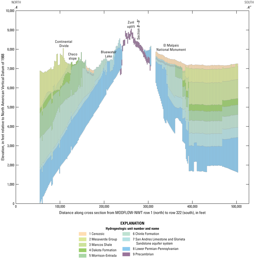
Cross section A–A′, oriented north to south, through the Rio San Jose Integrated Hydrologic Model.
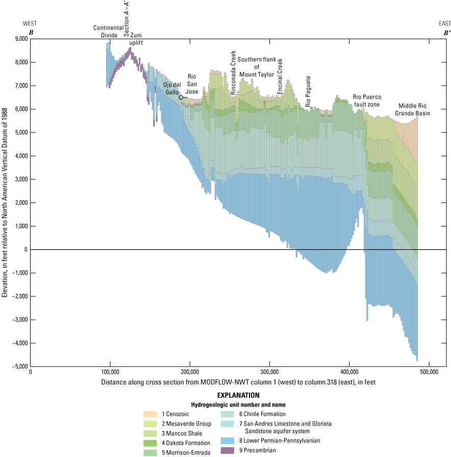
Cross section B–B′, oriented west to east, through the Rio San Jose Integrated Hydrologic Model.
The number of active layers at a model row and column location in MODFLOW-NWT was equal to the number of hydrogeologic units 1 to 8 (excluding the Precambrian hydrogeologic unit) that had a nonzero thickness in the geologic framework model (figs. 4 and 5). An arbitrary thickness value of 5 m was assigned where a geologic framework model unit was absent in the subsurface because of an erosional unconformity and between two units that were present (Sweetkind and others, 2020). In MODFLOW-NWT, the thickness of these absent hydrogeologic units was set as an active layer and had hydraulic properties assigned with the adjacent hydrogeologic unit (below) that was present. Because of the discontinuous nature of hydrogeologic units throughout the study area (table 4) (Sweetkind and others, 2020), MODFLOW-NWT layers represent multiple hydrogeologic units.
Model Parameterization
The locations of the faults, volcanic vents, and igneous dikes were incorporated in MODFLOW-NWT as areas of potential resistance to horizontal flow using the Horizontal Flow Barrier package (Hsieh and Freckleton, 1993) (plate 1). Eight calibration parameters were defined for the hydraulic characteristic within the Horizontal Flow Barrier package, one each for volcanic vents and igneous dikes and six for faults. The six fault parameters were created by grouping the faults on the basis of age (offsets pre-Quaternary units or Quaternary units) and fault strike (northwest, north, and northeast), with the groupings designed to combine faults with similar age and tectonic setting on the assumption that these similarities might result in similar fault behavior in restricting horizontal flow.
Multiple hydrogeologic unit zones were defined for 5 of the 9 hydrogeologic units by geologic framework model unit and previous studies that delineated distinct zones with similar hydraulic properties (horizontal hydraulic conductivity, vertical anisotropy, specific storage, and specific yield) within units (table 4 and figs. 6–10). The remaining 4 hydrogeologic units (Mancos Shale, Dakota Formation, Chinle Formation, Precambrian) were each assigned a single hydrogeologic unit zone (homogeneous hydraulic properties within the entire extent of the hydrogeologic unit) largely because of a lack of data from previous studies to inform spatial variability of hydraulic properties.
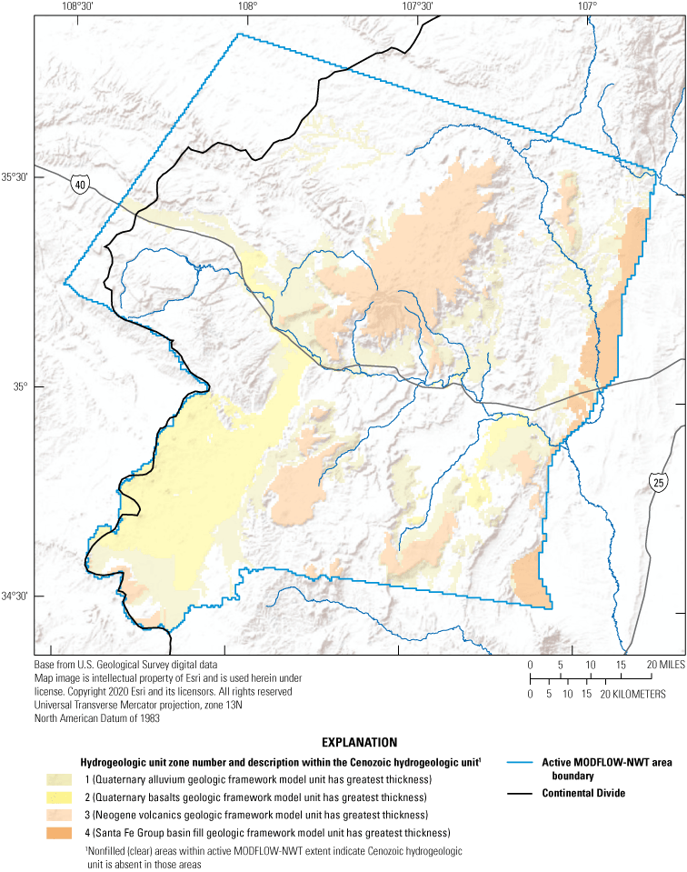
Four hydrogeologic unit zones defined in this study within the Cenozoic hydrogeologic unit on the basis of the geologic framework model unit that had the greatest thickness in each hydrogeologic unit to delineate regions with similar hydraulic properties (horizontal hydraulic conductivity, vertical anisotropy, specific storage, and specific yield) for the Rio San Jose Integrated Hydrologic Model, New Mexico.
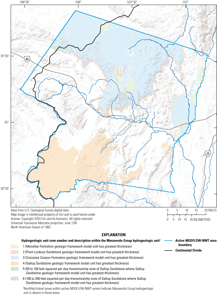
Six hydrogeologic unit zones defined in this study within the Mesaverde Group hydrogeologic unit on the basis of the geologic framework model unit that had the greatest thickness in each hydrogeologic unit and Stone (1981) to delineate regions with similar hydraulic properties (horizontal hydraulic conductivity, vertical anisotropy, specific storage, and specific yield) for the Rio San Jose Integrated Hydrologic Model, New Mexico.
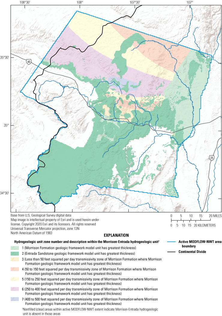
Seven hydrogeologic unit zones defined in this study within the Morrison-Entrada hydrogeologic unit on the basis of the geologic framework model unit that had the greatest thickness in each hydrogeologic unit and Frenzel and Lyford (1982) to delineate regions with similar hydraulic properties (horizontal hydraulic conductivity, vertical anisotropy, specific storage, and specific yield) for the Rio San Jose Integrated Hydrologic Model, New Mexico.
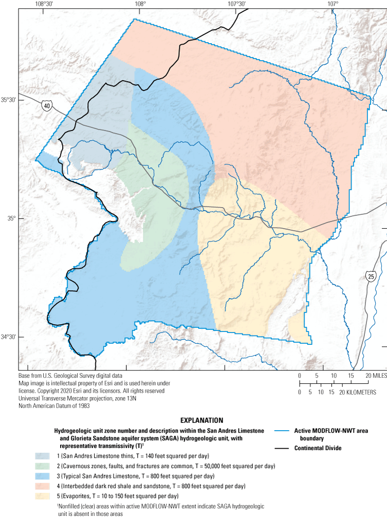
Five hydrogeologic unit zones defined in this study within the San Andres Limestone and Glorieta Sandstone aquifer system hydrogeologic unit on the basis of previous studies by Kelley and Wood (1946), Baars (1962), and Baldwin and Anderholm (1992) to delineate regions with similar hydraulic properties (horizontal hydraulic conductivity, vertical anisotropy, specific storage, and specific yield) for the Rio San Jose Integrated Hydrologic Model, New Mexico.
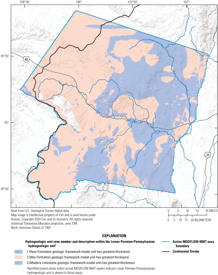
Three hydrogeologic unit zones defined in this study within the Lower Permian-Pennsylvanian hydrogeologic unit on the basis of the geologic framework model unit that had the greatest thickness in each hydrogeologic unit to delineate regions with similar hydraulic properties (horizontal hydraulic conductivity, vertical anisotropy, specific storage, and specific yield) for the Rio San Jose Integrated Hydrologic Model, New Mexico.
The Cenozoic and Lower Permian-Pennsylvanian hydrogeologic units were subdivided into 4 and 3 hydrogeologic unit zones, respectively (table 4, figs. 6 and 10), on the basis of the geologic framework model unit that had the greatest thickness in each hydrogeologic unit. The Mesaverde Group and Morrison-Entrada hydrogeologic units were subdivided into 6 and 7 hydrogeologic unit zones, respectively (figs. 7 and 8), on the basis of the geologic framework model unit that had the greatest thickness in each hydrogeologic unit and reported transmissivity zones (Stone, 1981; Frenzel and Lyford, 1982). Two transmissivity zones (50–100 and 100–350 feet squared per day [ft2/d]) for the Gallup Sandstone in the San Juan structural basin that were developed by Stone (1981) were used to subdivide the Mesaverde Group hydrogeologic unit. Five transmissivity zones (less than 50, 50–150, 150–250, 250–400, and 400–500 ft2/d) for the Morrison Formation in the San Juan structural basin that were developed by Frenzel and Lyford (1982) were used to subdivide the Morrison-Entrada hydrogeologic unit.
The SAGA hydrogeologic unit was subdivided into five hydrogeologic unit zones (fig. 9) on the basis of previous studies by Kelley and Wood (1946), Baars (1962), and Baldwin and Anderholm (1992). Hydrogeologic unit zone number 3 represents the typical San Andres Limestone, with the lower half to two-thirds usually a thin- to medium-bedded alternation of dolomites, shales, siltstones, and sandstones, overlain by a middle white sandstone and an overlying typically massive limestone. The San Andres Limestone in hydrogeologic unit zone number 3 was never exposed to subaerial erosion, so there are few solution-enhanced openings or caverns. Hydrogeologic unit zone number 3 is relatively distant from the faulting in the area of the community of Grants, so there is relatively limited secondary fracturing. Baldwin and Anderholm (1992) estimated the transmissivity of hydrogeologic unit zone number 3 to be 800 ft2/d on the basis of aquifer-test results from a single well. Hydrogeologic unit zone number 1 is like the typical San Andres Limestone in hydrogeologic unit zone number 3, except the San Andres Limestone thins such that more of the SAGA hydrogeologic unit hydraulic properties represent the Glorieta Sandstone. Baldwin and Anderholm (1992) reported transmissivity values ranging from 30 to 280 ft2/d and estimated a representative transmissivity of 140 ft2/d in hydrogeologic unit zone number 1. In hydrogeologic unit zone number 2, cavernous zones, faults, and fractures are common, and the large range in reported transmissivity (100–450,000 ft2/d) reflects well completions in various configurations of the faulted, fractured, and cavernous carbonate terrain. Baldwin and Anderholm (1992) estimated an average transmissivity of 50,000 ft2/d for hydrogeologic unit zone number 2. The San Andres Limestone changes abruptly to interbedded dark red shale and sandstone toward the north and northeast in hydrogeologic unit zone number 4. Although thin carbonates are usually present in hydrogeologic unit zone number 4, they are a minor feature. Baldwin and Anderholm (1992) estimated a representative transmissivity of 800 ft2/d in hydrogeologic unit zone number 4, but no wells were analyzed. The San Andres Limestone changes abruptly to evaporites toward the southeast in hydrogeologic unit zone number 5, thickening markedly into an evaporite basin (Baars, 1962). Kelley and Wood (1946) described a thick series of evaporites in the Sierra Lucero uplift of hydrogeologic unit zone number 5 that may be equivalent to the lower dolomites and clastics in the Zuni uplift. On the basis of lithologic and hydrologic data from seven wells, the transmissivity for hydrogeologic unit zone number 5 was estimated by Baldwin and Anderholm (1992) to range from 10 to 150 ft2/d.
Water Use Estimation and Distribution
Water use in the study area has varied both by category of use and quantity throughout the simulation periods of the RSJIHM. Although available data are sparse for some areas and years, effort was taken to accurately represent the water use changes that took place within the active MODFLOW-NWT area. Water use, including pumping, deep percolation, injection of water and seepage to groundwater from tailing piles related to uranium mill operations, and seepage to groundwater from water supply treatment plants, was simulated in MODFLOW-NWT using the Well package. Pumping was simulated using extraction wells, and deep percolation, injection, and seepage were simulated using injection wells (fig. 11). In addition, diversions of surface water from Bluewater Creek below Bluewater Dam for irrigation within the Bluewater-Toltec Irrigation District were simulated in MODFLOW-NWT as diversions from the SFR2 package.
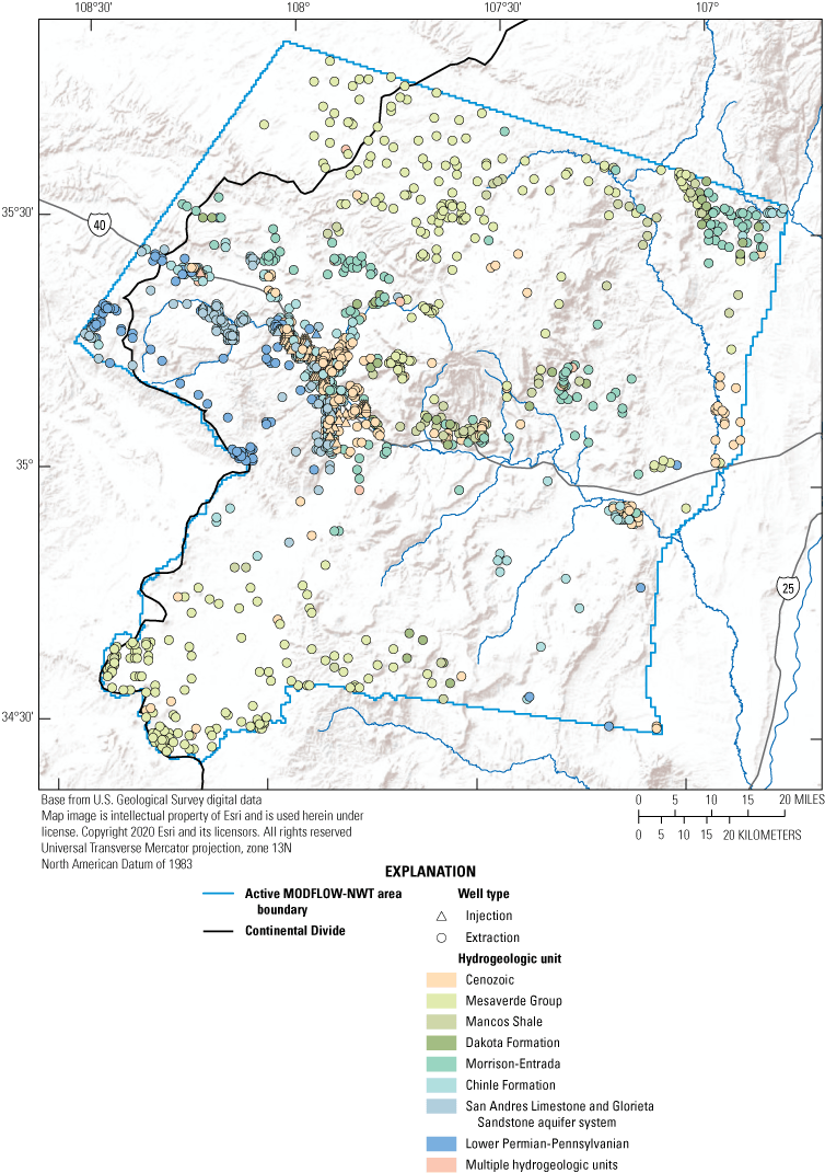
Locations of wells used to simulate injections and extractions to selected hydrogeologic units using the Well package for the transient MODFLOW-NWT.
Municipal and Industrial
Municipal and industrial water use was incorporated in the transient simulation period of MODFLOW-NWT and was based on a preliminary historical surface-water and groundwater use compilation for the Bluewater Declared Underground Water Basin (data are available on request from the NMOSE). The focus of the compilation was on the portion of the Bluewater Declared Underground Water Basin that was declared in 1956 and areas with municipal and industrial water development near the communities of Prewitt and Thoreau. The compilation contains monthly water use for 1945 through 2015. Municipal and industrial water use in the compilation was largely sourced from the NMOSE meter records and previous modeling efforts (Frenzel, 1992). The water use data from the compilation were checked against data acquired from other sources (Milan; Grants; NMOSE, 2019), and the meter records were checked for errors and corrected if needed. Meter data were used to extend the water use through 2018 when available (NMOSE, 2019). When no meter data were available, the data for the last available year were repeated for missing years.
Municipal water use for the Acoma Pueblo was included in MODFLOW-NWT using estimates based on reported and acquired pumping records (Shomaker and Coward, 2007; S. Juanico, Pueblo of Acoma, written commun., 2019). Industrial water use by the L-Bar mill also was included in MODFLOW-NWT using meter records obtained from the NMOSE (data are available on request from the NMOSE). Seepage to groundwater from water supply treatment plants near the communities of San Rafael and Thoreau was incorporated in MODFLOW-NWT on the basis of data in the preliminary historical surface-water and groundwater use compilation for the Bluewater Declared Underground Water Basin (data are available on request from the NMOSE).
Irrigation
Irrigation water use was incorporated in the steady-state and transient simulation periods of MODFLOW-NWT and was based on the preliminary historical surface-water and groundwater use compilation for the Bluewater Declared Underground Water Basin (data are available on request from the NMOSE), which uses data from a previous modeling effort (Frenzel, 1992) for 1945–85 and then applies the same irrigation water-balance approach to estimate water use through year 2015. The irrigation water-balance approach uses an estimate of irrigated acres and an average irrigation rate per acre to calculate the irrigation water demand, then uses surface-water supply to determine how much of the demand is met by surface water. The remaining irrigation demand is assumed to be met through groundwater pumping. The pumping is distributed equally to the wells (hereafter referred to as “Points of Diversion” [PODs]) in each irrigation area. Three years of the estimated irrigated acres from the compilation were checked using Landsat imagery and the Normalized Difference Vegetation Index (Masek and others, 2006; Vermote and others, 2016) to validate the irrigated acres from the compilation; estimates of irrigated acres were similar. Irrigation water use for 2015 was used for the years 2016 through 2018.
In the steady-state simulation period, groundwater pumping for irrigation in the Bluewater-Toltec Irrigation District was simulated as the average annual estimated groundwater withdrawal from 1944 through 1949, equally distributed to the irrigation wells in the Bluewater-Toltec Irrigation District (data are available on request from the NMOSE). Deep percolation in the Bluewater-Toltec Irrigation District and the region of the community of San Rafael was simulated in the steady-state simulation period as the average annual estimated deep percolation in each region from 1944 through 1949, equally distributed among the injection wells in each region (data are available on request from the NMOSE). Data from the preliminary historical surface-water and groundwater use compilation for the Bluewater Declared Underground Water Basin (data are available on request from the NMOSE) were used to simulate groundwater pumping for irrigation and deep percolation in the transient simulation period. Deep percolation was incorporated in the transient simulation period in the area west of Bluewater Lake, the Bluewater-Toltec Irrigation District, the region of the community of San Rafael, and the community of Grants golf course (fig. 11).
A steady-state surface-water diversion from Bluewater Creek below Bluewater Dam for irrigation within the Bluewater-Toltec Irrigation District was specified as the average annual estimated surface-water diversion for irrigation from 1944 through 1949 (data are available on request from the NMOSE). In the transient simulation period, estimated daily surface-water diversions from Bluewater Creek below Bluewater Dam for irrigation within the Bluewater-Toltec Irrigation District (see “Precipitation-Runoff Modeling System, Water Use Estimation and Distribution” section) were simulated in MODFLOW-NWT as specified diversions in the SFR2 package such that the diversions were either entirely met if the amount of available streamflow was greater than or equal to the diversions or reduced to the amount of available streamflow (IPRIOR variable equal to 0). Streamflow was diverted from the first reach in the segment (ISEG variable equal to 98) upstream from the Bluewater-Toltec Irrigation District into a segment (ISEG variable equal to 636) with a single reach, no downstream segment (OUTSEG variable equal to 0) and no interaction with the groundwater system (STRHC1 variable equal to 0) such that all the diverted streamflow was removed from MODFLOW-NWT as consumptive use.
Mining
Dewatering from uranium mining is represented as pumping from wells in the transient simulation period of MODFLOW-NWT. The pumping rates for the Ambrosia Lake, Smith Lake, and Laguna subdistricts within the Grants uranium district were based on data obtained from various sources (Goad and others, 1980; NMOSE, 2019). The dewatering for each mine area was distributed equally to the PODs that correspond with each site (NMOSE, 2018). Dewatering data were not available for all years that the mines were active, so data were extrapolated linearly for years where no data were available.
Water use from the modern coal mines in the active MODFLOW-NWT area, Lee Ranch and El Segundo, also was included using meter records obtained from the NMOSE (data are available on request from the NMOSE; Jeff Peterson, NMOSE, written commun., 2019). Injection of water and seepage to groundwater from tailing piles at the Homestake and Bluewater mills also were incorporated in the transient simulation period on the basis of data in the preliminary historical surface-water and groundwater use compilation for the Bluewater Declared Underground Water Basin (data are available on request from the NMOSE).
Domestic and Livestock
County estimates of domestic water use from the NMOSE water-use reports from 1975–2015 were used to estimate domestic pumping in the transient simulation period of MODFLOW-NWT (Sorensen, 1977, 1982; Wilson, 1986, 1992; Wilson and Lucero, 1997; Wilson and others, 2003; Longworth and others, 2008, 2013; Magnuson and others, 2019). The NMOSE water use report method uses rural population and per capita use to calculate the total domestic use. In order to get estimates for years prior to 1975, the percent change in census county populations was applied backward from the 1975 water-use estimate. County estimates of livestock water use in the transient simulation period of MODFLOW-NWT were calculated using livestock estimates per county from the U.S. Census of Agriculture (U.S. Department of Agriculture National Agricultural Statistics Service, variously dated) and coefficients for water use by each livestock type (Magnuson and others, 2019).
Both the domestic and livestock county water-use estimates were divided by the total number of PODs for each water-use category in the county (NMOSE, 2018) and multiplied by the number of PODs for that water-use category in both the county and within the active MODFLOW-NWT area to get a water-use estimate for MODFLOW-NWT. The water-use estimates, which were available approximately every 5 years, were then linearly interpolated to produce annual estimates and distributed among active PODs for each water-use category proportionally using the total allocation for the POD.
The average monthly municipal water use for the community of Milan (NMOSE, 2019) was applied to the domestic water use to distribute the annual estimates to monthly estimates. The annual livestock water use was distributed into monthly water use using an equation for cattle water use and monthly climate averages for the community of Grants (National Academies of Sciences, Engineering, and Medicine, 2016).
Well Depth
The MODFLOW-NWT layer used for each well was determined using the geologic framework model and the depth of the well. Screen depths or well depths were used when available (NMOSE, 2019). When depth information was not available for domestic or livestock wells, the well depth was calculated as the median depth of the three nearest wells that have a reported well depth. In some instances, the MODFLOW-NWT layer that was determined using well depth information and the geologic framework model did not agree with well logs or documented aquifer information, and well logs or documented aquifer information was used to assign a layer to the well.
Calibration Approach and Datasets
Calibration of MODFLOW-NWT was performed using BeoPEST (version 13.6) (Schreüder, 2021). BeoPEST was run using the USGS Yeti supercomputer (U.S. Geological Survey Advanced Research Computing, 2021). The parameters adjusted during calibration were
-
horizontal hydraulic conductivity, vertical anisotropy, specific yield, and specific storage of model layers;
-
hydraulic conductance within the General-Head Boundary package;
-
hydraulic characteristic within the Horizontal Flow Barrier package;
-
hydraulic conductivity of the streambed and springbed within the SFR2 package;
-
elevation of the top of the streambed and springbed within the SFR2 package; and
-
lakebed leakance within the Lake package.
Horizontal hydraulic conductivity, vertical anisotropy, specific yield, and specific storage parameters were adjusted for groups of grid cells corresponding to the hydrogeologic unit zones in each model layer. General-head boundary hydraulic conductance was adjusted for 7 parameter groups of grid cells, consisting of 5 parameter groups that corresponded to the five regions of groundwater flow into the Middle Rio Grande Basin used in McAda and Barroll (2002) and 1 parameter group each for groundwater flow across the northern and western boundaries of MODFLOW-NWT (plate 1). Eight parameters were defined for the hydraulic characteristic within the Horizontal Flow Barrier package (see “Model Layering and Parameterization from Geologic Framework Model” section). Parameters within the SFR2 package were defined separately for all stream network grid cells within each of the 15 subbasins, the Rio Puerco upstream from its confluence with the Arroyo Chico, the Rio Puerco downstream from its confluence with the Arroyo Chico, Horace Springs, and all other springs. A single lakebed leakance parameter was defined for the 13 grid cells representing Bluewater Lake.
Adjustments to parameter values during calibration were based on the ability of model simulated values to reproduce measured, estimated, or reported values for several observation groups: (1) streamflow, (2) head, (3) springflow at Ojo del Gallo, (4) springflow at Horace Springs, (5) surface-water releases from Bluewater Lake, and (6) surface-water diversions for irrigation within the Bluewater-Toltec Irrigation District. Observation weights within PEST were applied to give relatively equal importance to each observation group. Within observation groups, values were given the same PEST observation weights, except for head values, which were given variable weights based on the assumed quality of the data. Higher weights were assigned to head data assumed to be of higher quality, such as data from NWIS that have documented accuracies; lower weights were assigned to head data assumed to be of lower quality, such as data from NMOSE POD records that do not have documented accuracies and may not represent static heads. The ability of MODFLOW-NWT to reproduce measured, estimated, or reported values is discussed in the “Model Performance” section.
Streamflow
The steady-state MODFLOW-NWT was not calibrated to measured streamflow because of a lack of data from 1944 through 1949. However, both the steady-state and transient MODFLOW-NWT were calibrated to the conceptual understanding of zero streamflow leaving the stream network draining the northern part of the El Malpais National Monument and flowing to the Rio San Jose. The mean monthly, monthly mean, and annual mean statistics for streamflow at the 12 streamgages (table 3, fig. 2) were used to calibrate the transient MODFLOW-NWT. Unlike the PRMS calibration, which used measured daily mean streamflow minus estimated daily base flow at Rio San Jose at Acoma and flow replacement at Bluewater Creek below Bluewater Dam, the transient MODFLOW-NWT was calibrated to the measured streamflow at Rio San Jose at Acoma and Bluewater Creek below Bluewater Dam.
Hydraulic Head
The steady-state MODFLOW-NWT was calibrated to the maximum measured head at the wells and the land surface elevation at the spring locations. The transient MODFLOW-NWT was calibrated and verified to 7,689 head measurements from 3,561 wells that draw water from both single and multiple layers and calibrated to 245 land surface elevations at 160 spring locations. Head measurements were compiled from these sources: (1) NWIS (USGS, 2018), (2) U.S. Department of Energy Legacy Management Geospatial Environmental Mapping System (U.S. Department of Energy, 2018), (3) a hydrologic report of the San Juan structural basin (Stone and others, 1983, table 1), (4) the environmental impact study for the Roca Honda mine (Roca Honda Resources, L.L.C., 2013, table A-1), (5) NMOSE POD records (NMOSE, 2018), and (6) the New Mexico Bureau of Geology and Mineral Resources interactive map (New Mexico Bureau of Geology and Mineral Resources, 2019). The head measurements included 3,561 initial measurements that were the first head measurement at each well and 4,128 drawdown measurements that were calculated as the change in head relative to the first head measurement. The drawdown measurements were included to focus the calibration on representing the overall trends in heads throughout the study area and to minimize the impact of potential effects of initial conditions. Six wells within the study area have long-term records of head measurements covering most of the transient simulation period of the RSJIHM (table 5). Head measurements from two of these wells (USGS site numbers 350346107521201 and 351304107543701) were excluded from the calibration to serve as verification for assessing the performance of the RSJIHM relative to heads.
Table 5.
Wells where long-term measurements of hydraulic head were used for calibration and verification of the transient MODFLOW-NWT.[Data from U.S. Geological Survey ([USGS] 2018). USGS, U.S. Geological Survey; RSJIHM, Rio San Jose Integrated Hydrologic Model; SAGA, San Andres Limestone and Glorieta Sandstone aquifer system]
Springflow at Ojo del Gallo
The steady-state MODFLOW-NWT was calibrated to the average reported springflow at Ojo del Gallo (5 ft3/s) from 1944 through 1949 (Gordon, 1961; Baldwin and Anderholm, 1992). The transient MODFLOW-NWT was calibrated to reported springflow at Ojo del Gallo:
-
1 ft3/s from 1950 through 1952 (Gordon, 1961),
-
0 ft3/s from 1953 through 1980 (Baldwin and Anderholm, 1992),
-
1 ft3/s from 1981 through 1985 (White, 1989; Baldwin and Rankin, 1995),
-
2 ft3/s in 1986 (Baldwin and Anderholm, 1992), and
-
0 ft3/s from 1987 through 2018 (Baldwin and Anderholm, 1992).
The springflow at Ojo del Gallo was often reported for a particular day or month during the year, but the reported springflow was assumed to apply to the entire year for calibration. The simulated annual mean (arithmetic mean of the semimonthly springflow for each year) springflow was compared to the reported springflow for calibration.
Springflow at Horace Springs
The steady-state MODFLOW-NWT simulated Horace Springs springflow was calibrated to the average estimated daily base flow from 1944 through 1949 at Rio San Jose at Acoma (see “Precipitation-Runoff Modeling System, Calibration Approach and Datasets” section), which is coincident with Horace Springs and where groundwater discharge is assumed to be the predominant source of springflow (Frenzel, 1992; Baldwin and Anderholm, 1992; Wolf, 2016). The transient MODFLOW-NWT simulated Horace Springs springflow was calibrated to the estimated daily base flow at Rio San Jose at Acoma. The simulated annual mean springflow was compared to the estimated annual mean (arithmetic mean of the estimated daily base flow for each year) springflow for calibration. Annual mean statistics were only included for years with daily base flow estimated on each day of the year.
Surface-Water Releases From Bluewater Lake
The steady-state MODFLOW-NWT was calibrated to an estimated average annual release from Bluewater Lake, which was calculated as the average of the annual mean streamflow statistic obtained from NWIS (USGS, 2019b) at Bluewater Creek below Bluewater Dam. The transient MODFLOW-NWT was calibrated to the estimated monthly releases from Bluewater Lake to minimize the difference between simulated and specified releases. Estimated monthly releases were calculated by summing the estimated daily releases from Bluewater Lake (see “Precipitation-Runoff Modeling System, Stream Network Delineation and Streamflow Routing” section) for each month.
Surface-Water Diversions for Irrigation Within the Bluewater-Toltec Irrigation District
The steady-state MODFLOW-NWT was calibrated to the estimated steady-state surface-water diversion from Bluewater Creek below Bluewater Dam for irrigation within the Bluewater-Toltec Irrigation District that was specified in the SFR2 package (see “MODFLOW-NWT, Water Use Estimation and Distribution” section). The transient MODFLOW-NWT was calibrated to the estimated monthly surface-water diversions for irrigation within the Bluewater-Toltec Irrigation District to minimize the occurrence of specified diversions being reduced, because the amount of available streamflow was less than the diversions. Estimated monthly diversions were calculated by summing the estimated daily surface-water diversions from Bluewater Creek below Bluewater Dam for irrigation within the Bluewater-Toltec Irrigation District (see “Precipitation-Runoff Modeling System, Water Use Estimation and Distribution” section) for each month.
Integrated Model Approach
The RSJIHM was developed by sequentially linking PRMS and MODFLOW-NWT. The sequentially linked integration is performed by running PRMS first and feeding PRMS simulated outputs (recharge, surface runoff to streams, and interflow from the soil zone to streams) into MODFLOW-NWT as inputs, and then running MODFLOW-NWT. Daily recharge to the groundwater reservoir (recharge variable) simulated by PRMS within each HRU was aggregated by month and applied to the equivalent grid cell in layer 1 of MODFLOW-NWT as a monthly rate using the Recharge package (Harbaugh and others, 2000). Daily surface runoff to streams (sroff variable) and interflow from the soil zone to streams (ssres_flow variable) simulated by PRMS were aggregated by segment and month and equally distributed to each reach in a segment as a monthly volumetric rate using the RUNOFF variable within the SFR2 package. The sequentially linked approach was chosen to approximate a fully coupled GSFLOW without the computational requirements (resulting in faster simulation run times) and the fully coupled feedbacks between PRMS and MODFLOW-NWT at a daily time step (resulting in simplification of the simulation of the hydrologic system). Despite not being coupled, the RSJIHM approximates how GSFLOW simulates flow within and among three regions: (1) the region from the top of the plant canopy to the bottom of the soil zone, including the snowpack and surface-depression storage (simulated by PRMS), (2) all streams and lakes (simulated by MODFLOW-NWT), and (3) the subsurface zone beneath the soil zone (simulated by MODFLOW-NWT).
Calibration Results
This section summarizes the calibrated PRMS and MODFLOW-NWT parameters. Selected MODFLOW-NWT parameters are discussed that affect the simulation of groundwater flow and groundwater/surface-water interaction in the RSJIHM. Hydraulic properties of MODFLOW-NWT layers, General-Head Boundary package hydraulic conductance, and Horizontal Flow Barrier package hydraulic characteristic affect the simulation of groundwater flow and groundwater/surface-water interaction. Streambed and springbed hydraulic conductivity within the SFR2 package and lakebed leakance within the Lake package affect groundwater/surface-water interaction.
Precipitation-Runoff Modeling System Results
During calibration, PRMS parameter values were allowed to vary within the range of possible values in PRMS (Markstrom and others, 2015). The resulting statistics (minimum, maximum, mean, median, and standard deviation) of calibrated PRMS parameters are presented in table 6.
Table 6.
Statistics of the calibrated Precipitation-Runoff Modeling System parameters for the Rio San Jose Integrated Hydrologic Model, New Mexico.[°F, degrees Fahrenheit; NA, not applicable]
MODFLOW-NWT Results
Hydraulic Properties of Model Layers
The horizontal hydraulic conductivity, vertical anisotropy, specific yield, and specific storage values by hydrogeologic unit and hydrogeologic unit zone that resulted from the calibration of the transient RSJIHM are presented in table 7. During calibration, the hydraulic conductivity and storage property values were allowed to vary within the range of reported hydraulic property values obtained from previous studies (table 7). The calibrated horizontal hydraulic conductivity ranged from 0.0065 to 80 ft/d. The lowest horizontal hydraulic conductivity value was associated with the Cenozoic hydrogeologic unit zone number 3 where Miocene to Pliocene basaltic to andesitic lava flows with local dacites near Mount Taylor of the Neogene volcanics geologic framework model unit are predominant. The highest horizontal hydraulic conductivity value was associated with SAGA hydrogeologic unit zone number 2 where cavernous zones, faults, and fractures are common. The calibrated vertical anisotropy (ratio of horizontal hydraulic conductivity divided by vertical hydraulic conductivity) ranged from 8.0 to 61,000. The lowest vertical anisotropy value was associated with Cenozoic hydrogeologic unit zone numbers 2 and 4 where the basaltic to andesitic lava flows and alluvial deposits of the Quaternary basalts geologic framework model unit and the Oligocene to early Pleistocene sedimentary and volcanic partly consolidated conglomerate sandstone, shale, volcanics of the Santa Fe Group basin fill geologic framework model unit are predominant, respectively. The highest vertical anisotropy value was associated with the Mesaverde Group hydrogeologic unit zone number 3 where shale, siltstone, and coal of the Crevasse Canyon Formation geologic framework model unit are predominant. Specific yield was calibrated to range from 0.020 to 0.29, and specific storage was calibrated to range from 1.0×10–08 to 4.0×10–05 per foot.
Table 7.
Calibrated and range of reported (in parenthesis if applicable) horizontal hydraulic conductivity, vertical anisotropy, specific yield, and specific storage by hydrogeologic unit and zone for the Rio San Jose Integrated Hydrologic Model, New Mexico.[ft2/d, foot squared per day; NA, not applicable; SAGA, San Andres Limestone and Glorieta Sandstone aquifer system]
| Hydro-geologic unit name | Hydro-geologic unit zone number | Hydrogeologic unit zone description | Hydrogeologic unit zone thickness range (feet) |
Source of reported hydraulic property values used to constrain PEST calibration | Horizontal hydraulic conductivity (feet per day) |
Vertical anisotropy (unitless) | Specific yield (unitless) |
Specific storage (foot-1) |
|---|---|---|---|---|---|---|---|---|
| Cenozoic | 1 | Quaternary alluvium geologic framework model unit has greatest thickness in Cenozoic hydrogeologic unit | 114–387 | Ward and others (1982), Risser and Lyford (1983), Risser and others (1984), Baldwin and Anderholm (1992), U.S. Department of Energy (2014) |
56 (0.20–700) | 73 | 0.26 (0.10 to 0.25) | 2.0×10−07 |
| Cenozoic | 2 | Quaternary basalts geologic framework model unit has greatest thickness in Cenozoic hydrogeologic unit | 65–1,060 | Risser and Lyford (1983), U.S. Department of Energy (2014) |
10 (6.9–130) | 8.0 | 0.020 | 3.4×10−06 |
| Cenozoic | 3 | Neogene volcanics geologic framework model unit has greatest thickness in Cenozoic hydrogeologic unit | 51–2,563 | INTERA, Inc. (2012), Langman and others (2012) |
0.0065 (0.00010–1,000) | 61 | 0.094 | 4.4×10−06 |
| Cenozoic | 4 | Santa Fe Group basin fill geologic framework model unit has greatest thickness in Cenozoic hydrogeologic unit | 35–5,632 | Risser and Lyford (1983) | 0.29 (0.86) | 8.0 | 0.033 | 1.2×10−06 |
| Mesaverde Group | 1 | Menefee Formation geologic framework model unit has greatest thickness in Mesaverde Group hydrogeologic unit | 1,102–3,158 | Frenzel and Lyford (1982), Kernodle (1996), INTERA, Inc. (2012), Langman and others (2012) |
0.18 (0.001–1.0) | 2,400 | 0.020 | 1.8×10−07 |
| Mesaverde Group | 2 | Point Lookout Sandstone geologic framework model unit has greatest thickness in Mesaverde Group hydrogeologic unit | 757–2,236 | Brod (1979), Brod and Stone (1981), Frenzel and Lyford (1982), Kernodle (1996), INTERA, Inc. (2012), Langman and others (2012) |
0.0080 (0.0020–1.5) | 5,700 | 0.13 | 3.7×10−06 |
| Mesaverde Group | 3 | Crevasse Canyon Formation geologic framework model unit has greatest thickness in Mesaverde Group hydrogeologic unit | 133–3,191 | Frenzel and Lyford (1982), INTERA, Inc. (2012), Langman and others (2012) |
0.097 (0.0020–1.0) | 61,000 | 0.18 | 2.8×10−06 |
| Mesaverde Group | 4 | Gallup Sandstone geologic framework model unit has greatest thickness in Mesaverde Group hydrogeologic unit | 65–1,255 | Brod (1979), Frenzel and Lyford (1982), Ward and others (1982), INTERA, Inc. (2012), Langman and others (2012) |
0.18 (0.10–1.5) | 1,100 | 0.081 | 9.6×10−07 |
| Mesaverde Group | 5 | 50 to 100 ft2/d transmissivity zone of Gallup Sandstone where Gallup Sandstone geologic framework model unit has greatest thickness in Mesaverde Group hydrogeologic unit | 161–1,320 | Stone (1981) | 1.3 | 800 | 0.031 | 1.0×10−06 |
| Mesaverde Group | 6 | 100 to 350 ft2/d transmissivity zone of Gallup Sandstone where Gallup Sandstone geologic framework model unit has greatest thickness in Mesaverde Group hydrogeologic unit | 82–4,275 | Stone (1981) | 0.51 | 800 | 0.20 | 3.4×10−06 |
| Mancos Shale | 1 | Mancos Shale | 32–2,161 | Brod (1979), Brod and Stone (1981), Frenzel and Lyford (1982), Ward and others (1982), INTERA, Inc. (2012), Langman and others (2012) |
0.069 (0.00010–2.7) | 100 | 0.031 | 5.3×10−07 |
| Dakota Formation | 1 | Dakota Formation | 33–983 | Brod (1979), Brod and Stone (1981), Ward and others (1982), Risser and Lyford (1983), Stone and others (1983), Kernodle (1996), INTERA, Inc. (2012), Langman and others (2012) |
0.11 (0.00040–100) | 5,400 | 0.052 | 1.4×10−07 (1.7×10−07) |
| Morrison-Entrada | 1 | Morrison Formation geologic framework model unit has greatest thickness in Morrison-Entrada hydrogeologic unit | 99–1,510 | Brod (1979), Brod and Stone (1981), Frenzel and Lyford (1982), Ward and others (1982), Risser and Lyford (1983), Stone and others (1983), Risser and others (1984), INTERA, Inc. (2012), Langman and others (2012) |
50 (0.00080–52) | 100 | 0.020 | 2.2×10−06 (1.3×10−07 to 3.7×10−05) |
| Morrison-Entrada | 2 | Entrada Sandstone geologic framework model unit has greatest thickness in Morrison-Entrada hydrogeologic unit | 34–1,625 | Frenzel and Lyford (1982), Kernodle (1996), Langman and others (2012) |
0.050 (0.41–18) | 1,700 | 0.020 | 2.9×10−05 |
| Morrison-Entrada | 3 | Less than 50 ft2/d transmissivity zone of Morrison Formation where Morrison Formation geologic framework model unit has greatest thickness in Morrison-Entrada hydrogeologic unit | 88–1,312 | Frenzel and Lyford (1982) | 0.010 | 130 | 0.043 | 4.0×10−07 |
| Morrison-Entrada | 4 | 50 to 150 ft2/d transmissivity zone of Morrison Formation where Morrison Formation geologic framework model unit has greatest thickness in Morrison-Entrada hydrogeologic unit | 318–1,538 | Frenzel and Lyford (1982) | 1.0 | 5,000 | NA | 5.4×10−06 |
| Morrison-Entrada | 5 | 150 to 250 ft2/d transmissivity zone of Morrison Formation where Morrison Formation geologic framework model unit has greatest thickness in Morrison-Entrada hydrogeologic unit | 209–1,641 | Frenzel and Lyford (1982) | 0.11 | 100 | NA | 8.8×10−06 |
| Morrison-Entrada | 6 | 250 to 400 ft2/d transmissivity zone of Morrison Formation where Morrison Formation geologic framework model unit has greatest thickness in Morrison-Entrada hydrogeologic unit | 119–1,723 | Frenzel and Lyford (1982) | 4.0 | 3,200 | 0.020 | 3.7×10−05 |
| Morrison-Entrada | 7 | 400 to 500 ft2/d transmissivity zone of Morrison Formation where Morrison Formation geologic framework model unit has greatest thickness in Morrison-Entrada hydrogeologic unit | 189–1,528 | Frenzel and Lyford (1982) | 7.5 | 10,000 | NA | 4.0×10−05 |
| Chinle Formation | 1 | Chinle Formation | 33–2,658 | Ward and others (1982), Risser and Lyford (1983), Baldwin and Anderholm (1992), Langman and others (2012) |
0.070 (1.0×10-08–0.10) | 110 | 0.032 | 3.2×10−07 |
| SAGA | 1 | Like SAGA hydrogeologic unit zone number 3, except the San Andres Limestone thins such that more of SAGA hydrogeologic unit hydraulic properties may be governed by the Glorieta Sandstone | 33–819 | Baldwin and Anderholm (1992) | 1.3 | 90 | 0.17 | 7.3×10−08 |
| SAGA | 2 | Cavernous zones, faults, and fractures are common | 33–818 | Baldwin and Anderholm (1992) | 80 | 59 | 0.020 | 3.4×10−08 |
| SAGA | 3 | Typical San Andres Limestone | 33–819 | Baldwin and Anderholm (1992) | 0.14 | 20 | 0.12 | 1.0×10−06 |
| SAGA | 4 | The San Andres Limestone changes abruptly to interbedded dark red shale and sandstone toward the north and northeast. Although thin carbonates are usually present, they are a minor feature. | 33–820 | Baldwin and Anderholm (1992) | 0.024 | 1,000 | NA | 1.0×10−08 |
| SAGA | 5 | The San Andres Limestone changes abruptly to evaporites toward the southeast. | 37–819 | Baldwin and Anderholm (1992) | 0.025 | 1,000 | 0.036 | 8.3×10−07 |
| Lower Permian-Pennsylvanian | 1 | Yeso Formation geologic framework model unit has greatest thickness in Lower Permian-Pennsylvanian hydrogeologic unit | 82 | Baldwin and Anderholm (1992) | 0.068 (0.00030–0.6) | 34 | 0.020 | 2.7×10−06 |
| Lower Permian-Pennsylvanian | 2 | Abo Formation geologic framework model unit has greatest thickness in Lower Permian-Pennsylvanian hydrogeologic unit | 82–10,602 | Baldwin and Anderholm (1992) | 0.057 (0.00030–0.6) | 650 | 0.21 | 1.0×10−07 |
| Lower Permian-Pennsylvanian | 3 | Madera Limestone geologic framework model unit has greatest thickness in Lower Permian-Pennsylvanian hydrogeologic unit | 125–4,920 | Baldwin and Anderholm (1992) | 0.023 (0.00050–1.0) | 22 | 0.29 | 1.6×10−06 |
| Precambrian | 1 | Precambrian | 300 | NA | 0.30 | 28 | 0.020 | 1.0×10−07 |
General-Head Boundary Hydraulic Conductance
The General-Head Boundary package hydraulic conductance values that resulted from the calibration of the transient RSJIHM are presented in table 8. During calibration, the hydraulic conductance values were allowed to vary within a range of 10 orders of magnitude because of a lack of data to constrain the values. The calibrated hydraulic conductance ranged from 0.000036 ft2/d along the western boundary to 68 ft2/d along the Rio Salado region of the Middle Rio Grande Basin boundary used in McAda and Barroll (2002) (plate 1).
Table 8.
Calibrated General-Head Boundary package hydraulic conductance values for the Rio San Jose Integrated Hydrologic Model, New Mexico.[MRGB, Middle Rio Grande Basin]
Horizontal Flow Barrier Hydraulic Characteristic
The Horizontal Flow Barrier package hydraulic characteristic values that resulted from the calibration of the transient RSJIHM are presented in table 9. During calibration, the hydraulic characteristic values were allowed to vary within a range of 10 orders of magnitude because of a lack of data to constrain the values. The calibrated hydraulic characteristic ranged from 0.00000000010 per day for faults that offset pre-Quaternary units and have a general northwest strike to 0.070 per day for volcanic vents (plate 1). The faults with the highest calibrated hydraulic characteristic were those that offset pre-Quaternary units and have a general northeast strike and extend from El Malpais National Monument to the north and northeast of the community of Grants. The faults with the lowest calibrated hydraulic characteristic tended to be those that are along and near the boundaries of the active MODFLOW-NWT area.
Table 9.
Calibrated Horizontal Flow Barrier package hydraulic characteristic values for the Rio San Jose Integrated Hydrologic Model, New Mexico.Streambed and Springbed Hydraulic Conductivity
The streambed and springbed hydraulic conductivity values that resulted from the calibration of the transient RSJIHM are presented in table 10. During calibration, the streambed and springbed hydraulic conductivity values were allowed to vary within the range of reported horizontal hydraulic conductivity values obtained from previous studies (table 7). The calibrated streambed hydraulic conductivity ranged from 0.000010 ft/d in subbasin 11 to 77 ft/d in subbasin 2. The calibrated springbed hydraulic conductivity ranged from 10 ft/d at Horace Spring to 27 ft/d at all other springs.
Table 10.
Calibrated streambed and springbed hydraulic conductivity for the Rio San Jose Integrated Hydrologic Model, New Mexico.Streambed and Springbed Elevation
The elevation of the top of the streambed and springbed as derived from the GSFLOW-Arcpy toolkit (set as 1 ft below the adjusted HRU land surface elevations described in the “Precipitation-Runoff Modeling System” section) was calibrated by optimizing reductions to the elevation (table 11). During calibration, the elevation reductions were allowed to vary from 1 ft to the reduction that would cause the bed of at least one reach in a parameter group to fall below the uppermost model layer. The calibrated elevation reductions ranged from 1.0 ft in subbasin 12 to 82 ft in subbasin 1. The highest calibrated elevation reductions tended to be for reaches in higher elevation subbasins where greater slopes result in a larger range of elevations within the 500- by 500-m grid cells (USGS, 2017). Therefore, the horizontal discretization of the RSJIHM was too coarse in these areas to accurately represent the streambed elevation without adjustment.
Table 11.
Calibrated reductions to the elevation of the top of the streambed and springbed for the Rio San Jose Integrated Hydrologic Model, New Mexico.Model Performance
The performance of the RSJIHM is discussed by evaluating mass balance errors and comparing model simulated values against measured, estimated, or reported values. The mass balance errors quantify the accuracy of the matrix solution associated with the simulation and provide context for the uncertainty of various hydrologic budget components (Reilly and Harbaugh, 2004). The performance of the RSJIHM to simulate measurements and physically based estimates of solar radiation, potential evapotranspiration, actual evapotranspiration, precipitation and minimum and maximum air temperature, snow water equivalent, snow-covered area, and streamflow was evaluated using quantitative performance measures and graphical methods (Harmel and others, 2014; Moriasi and others 2015; Harmel and others, 2018). The quantitative performance was evaluated using the Nash-Sutcliffe model efficiency coefficient, percent bias, and coefficient of determination (R2). Moriasi and others (2015, table 9), provided performance evaluation criteria ranging from “not satisfactory” to “very good” for these quantitative measures for watershed-scale flow models. The Nash-Sutcliffe model efficiency coefficient can range from negative infinity to 1, with the optimal value being 1 (Moriasi and others, 2015). The percent bias can range from −100 to 100 percent, with negative values indicating undersimulation (simulated less than measured/estimated), positive values indicating oversimulation (simulated greater than measured/estimated), and the optimal value being 0 (Moriasi and others, 2015). The R2 can range from 0 to 1, with the optimal value being 1 (Moriasi and others, 2015).
Mass Balance
The MODFLOW-NWT mass balance of the steady-state simulation period was evaluated using percent error. The MODFLOW-NWT mass balance of the transient simulation period was evaluated using percent and absolute volume errors for all 1,650 semimonthly time steps and annual absolute volume errors from 1950 through 2018. The percent error was calculated as
whereVi
is the sum of all volumetric rate inflows to the groundwater system for each time step, and
Vo
is the sum of all volumetric rate outflows from the groundwater system for each time step.
The absolute volume error for each time step was calculated as
whereThe annual absolute volume error was calculated by summing all absolute volume errors for each time step in a calendar year.
For the steady-state simulation period (1944 through 1949), the percent error was calculated to be 0 percent. For the transient simulation period (1950 through 2018), the average percent error for all time steps was calculated to be −0.026 percent, indicating a slight bias towards more outflows than inflows. The minimum, maximum, and standard deviation of percent errors were −13 percent, 1.8 percent, and 0.53 percent, respectively. The average absolute volume error for all time steps was 7.2 acre-feet (acre-ft), and the average annual absolute volume error was 170 acre-ft. The minimum, maximum, and standard deviation of annual absolute volume errors were 6.5, 800, and 150 acre-ft, respectively. The greatest mass balance errors were scattered throughout the simulation period of the RSJIHM, indicating minimal temporal bias associated with mass balance errors. Overall, the mass balance errors represented a small fraction of the total inflows and outflows (annual absolute volume errors represented a maximum of 0.61 percent of annual total inflows or outflows) simulated by the RSJIHM, and most hydrologic budget components were greater than the uncertainty generated by these errors.
Solar Radiation
The Nash-Sutcliffe model efficiency coefficient between measured and simulated solar radiation ranged from 0.92 in subbasin 8 to 0.99 in subbasins 11 and 12 and was 0.97 (“very good”) for all subbasins (table 12). The percent bias between measured and simulated solar radiation ranged from −2.2 in subbasin 7 to 2.4 in subbasin 8 and was zero (“very good”) for all subbasins. The R2 between measured and simulated solar radiation was 0.96 (“very good”) for all subbasins. Overall, the quantitative measures indicate RSJIHM performance was “very good” in simulating measured solar radiation throughout the active PRMS area.
Table 12.
Statistics summarizing the calibration of Precipitation-Runoff Modeling System to measured or estimated values of solar radiation, potential evapotranspiration, and actual evapotranspiration by subbasin for the Rio San Jose Integrated Hydrologic Model, New Mexico.[NSE, Nash-Sutcliffe model efficiency coefficient; R2, coefficient of determination; PB, percent bias; NA, not applicable. Performance evaluation criteria for watershed-scale flow models from Moriasi and others (2015, table 9) are defined as follows: NSE > 0.80 = "very good," 0.70 < NSE ≤ 0.80 = "good," 0.50 < NSE ≤ 0.70 = "satisfactory," and NSE ≤ 0.50 = "not satisfactory"; PB < ±5 = "very good," ±5 ≤ PB < ±10 = "good," ±10 ≤ PB < ±15 = "satisfactory," and PB ≥ ±15 = "not satisfactory"; R2 > 0.85 = "very good," 0.75 < R2 ≤ 0.85 = "good," 0.60 < R2 ≤ 0.75 = "satisfactory," and R2 ≤ 0.60= "not satisfactory"]
Potential Evapotranspiration
The Nash-Sutcliffe model efficiency coefficient between estimated and simulated potential evapotranspiration ranged from 0.85 in subbasin 1 to 0.97 in subbasin 11 and was 0.93 (“very good”) for all subbasins (table 12). The percent bias between estimated and simulated potential evapotranspiration ranged from −13 (“satisfactory”) in subbasin 1 to 11 (“satisfactory”) in subbasin 2 and was 1.4 (“very good”) for all subbasins. Nine of the 15 subbasins had percent bias between estimated and simulated potential evapotranspiration less than ±5 (“very good”) and 4 of the subbasins had percent bias between estimated and simulated potential evapotranspiration from ±5 to less than ±10 (“good”). The R2 between estimated and simulated potential evapotranspiration was 0.94 (“very good”) for all subbasins. Overall, these quantitative measures indicate RSJIHM performance was “satisfactory” to “very good” in simulating estimated potential evapotranspiration throughout the active PRMS area.
Actual Evapotranspiration
The Nash-Sutcliffe model efficiency coefficient between estimated and simulated actual evapotranspiration ranged from −1.5 in subbasin 10 to 0.38 in subbasin 7 and was −0.12 (“not satisfactory”) for all subbasins where estimated actual evapotranspiration data were available (subbasins 1–3 and 5–12) (table 12). The percent bias between estimated and simulated actual evapotranspiration ranged from 11 (“satisfactory”) in subbasin 9 to 78 (“not satisfactory”) in subbasin 10 and was 26 (“not satisfactory”) for all subbasins where estimated actual evapotranspiration data were available, indicating that PRMS simulated more evapotranspiration than the estimated values. The R2 between estimated and simulated actual evapotranspiration ranged from 0.25 (“not satisfactory”) in subbasin 9 to 0.81 (“good”) in subbasin 3 and was 0.53 (“not satisfactory”) for all subbasins where estimated actual evapotranspiration data were available.
Overall, these quantitative measures indicate RSJIHM performance was “not satisfactory” to “good” in simulating estimated actual evapotranspiration throughout the active PRMS area. The performance of the RSJIHM at simulating estimated actual evapotranspiration was worst during the months of April and May in the higher elevation subbasins 1 and 2 in the Zuni uplift and during the months of August through October in the lower elevation subbasins. However, the RSJIHM simulated the overall patterns of estimated actual evapotranspiration, including gradually increasing actual evapotranspiration from January through August and rapidly decreasing actual evapotranspiration from September through December.
Precipitation and Minimum and Maximum Air Temperature
The Nash-Sutcliffe model efficiency coefficient between measured and simulated monthly total precipitation ranged from −0.65 (“not satisfactory”) to 0.92 (“very good”) and was 0.78 (“good”) for all climate stations (table 13). Nine of the 12 climate stations had Nash-Sutcliffe model efficiency coefficients rated at least “satisfactory.” The percent bias between measured and simulated monthly total precipitation ranged from −18 (“not satisfactory”) to 57 (“not satisfactory”) and was 4.8 (“very good”) for all climate stations. Seven of the 12 climate stations had percent bias rated at least “satisfactory.” The R2 between measured and simulated monthly total precipitation ranged from 0.35 (“not satisfactory”) to 0.98 (“very good”) and was 0.81 (“good”) for all climate stations.
Table 13.
Statistics summarizing the calibration of Precipitation-Runoff Modeling System to measured monthly total precipitation, monthly mean minimum air temperature, and monthly mean maximum air temperature at Global Historical Climatology Network-Monthly climate stations for the Rio San Jose Integrated Hydrologic Model, New Mexico.[NSE, Nash-Sutcliffe model efficiency coefficient; PB, percent bias. Performance evaluation criteria for watershed-scale flow models from Moriasi and others (2015, table 9) are defined as follows: NSE > 0.80 = "very good," 0.70 < NSE ≤ 0.80 = "good," 0.50 < NSE ≤ 0.70 = "satisfactory," and NSE ≤ 0.50 = "not satisfactory"; PB < ±5 = "very good," ±5 ≤ PB < ±10 = "good," ±10 ≤ PB < ±15 = "satisfactory," and PB ≥ ±15 = "not satisfactory"; R2 > 0.85 = "very good," 0.75 < R2 ≤ 0.85 = "good," 0.60 < R2 ≤ 0.75 = "satisfactory," and R2 ≤ 0.60= "not satisfactory"]
The Nash-Sutcliffe model efficiency coefficient between measured and simulated monthly mean minimum air temperature ranged from 0.78 (“good”) to 0.98 (“very good”) and was 0.94 (“very good”) for all climate stations (table 13). Eleven of the 12 climate stations had Nash-Sutcliffe model efficiency coefficients that were rated “very good.” The percent bias between measured and simulated monthly mean minimum air temperature ranged from −17 (“not satisfactory”) to 3.1 (“very good”) and was −0.10 (“very good”) for all climate stations. Ten of the 12 climate stations had percent bias that was rated “very good.” The R2 between measured and simulated monthly mean minimum air temperature ranged from 0.88 to 0.98 and was 0.94 (“very good”) for all climate stations.
The Nash-Sutcliffe model efficiency coefficient between measured and simulated monthly mean maximum air temperature ranged from 0.79 (“good”) to 0.97 (“very good”) and was 0.93 (“very good”) for all climate stations (table 13). Eleven of the 12 climate stations had Nash-Sutcliffe model efficiency coefficients that were rated “very good.” The percent bias between measured and simulated monthly mean maximum air temperature ranged from −7.5 (“good”) to 1.5 (“very good”) and was −1.7 (“very good”) for all climate stations. Ten of the 12 climate stations had percent bias that was rated “very good.” The R2 between measured and simulated monthly mean maximum air temperature ranged from 0.90 to 0.98 and was 0.94 (“very good”) for all climate stations.
Overall, these quantitative measures indicate the RSJIHM performance was “not satisfactory” to “very good” in simulating measured monthly total precipitation throughout the active PRMS area. The RSJIHM performed better at simulating measured monthly mean minimum and maximum air temperature with the quantitative measures generally rated “good” to “very good.”
Snow Water Equivalent
The Nash-Sutcliffe model efficiency coefficient between measured and simulated monthly mean snow water equivalent was 0.59 (“satisfactory”). The percent bias between measured and simulated monthly mean snow water equivalent was −58 (“not satisfactory”). The R2 between measured and simulated monthly mean snow water equivalent was 0.77 (“good”). Overall, these quantitative measures indicate the RSJIHM performance was “not satisfactory” to “good” in simulating measured monthly mean snow water equivalent at the Rice Park SNOTEL site. The RSJIHM was generally able to match the timing of the measured peak snow water equivalent. However, the RSJIHM generally undersimulated snow water equivalent (average of measured and simulated monthly mean snow water equivalent equal to 1.0 and 0.43 inches, respectively, from October 1, 1998, through September 30, 2018).
Snow-Covered Area
Because of the large range of estimated error bounds (see the “Precipitation-Runoff Modeling System, Calibration Approach and Datasets” section) on the daily, area-weighted average percent snow-covered area within each subbasin, qualitative methods rather than quantitative measures were used to evaluate the performance of the RSJIHM at simulating snow-covered area. The mean monthly simulated daily, area-weighted average snow-covered areas within the 15 subbasins are summarized in table 14. The simulated patterns of increased snow-covered area during December through March and decreased snow-covered area to near 0 percent during April through November are expected throughout the basin. Generally, the lower and upper error bounds indicated large ranges of uncertainty associated with the snow cover values derived from the MODIS. The simulated snow-covered area was generally closer to the upper error bound during January and February in the higher elevation subbasins 1 and 2 in the Zuni uplift and in subbasin 5 on the western flank of Mount Taylor and generally closer to the lower error bound during the other months. The simulated snow-covered area in the other subbasins was generally near the lower error bound for all months.
Table 14.
Mean monthly simulated daily, area-weighted average snow-covered area, in percent, by subbasin for the Rio San Jose Integrated Hydrologic Model, New Mexico.The spatial distribution of the mean monthly simulated snow-covered area by HRU during the peak snow cover month of January is shown in figure 12. The largest snow-covered areas are found in the higher elevation subbasins 1 and 2 in the Zuni uplift, exceeding 90 percent in some HRUs. Other large snow-covered areas are in higher elevations on the flanks of Mount Taylor and in the far northern portion of subbasin 7 within the Chaco slope subdivision of the San Juan structural basin. These results illustrate the elevation dependency of snow accumulation in the basin.
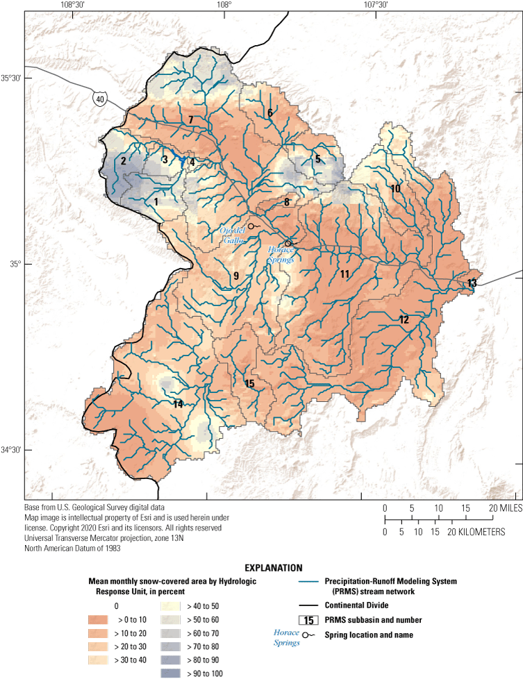
January mean monthly snow-covered area simulated by the Rio San Jose Integrated Hydrologic Model.
Streamflow
Mean Monthly
The Nash-Sutcliffe model efficiency coefficient between measured and simulated mean monthly streamflow ranged from −1.9 (“not satisfactory”) at the outlet of subbasin 5 to 0.99 (“very good”) at the outlet of subbasin 3 and was 0.53 (“satisfactory”) for all streamgages (table 15). The percent bias between measured and simulated mean monthly streamflow ranged from −100 at the outlets of subbasins 5 and 6 to 51 at the outlet of subbasin 2 (both “not satisfactory”) and was 2.8 (“very good”) for all streamgages. The R2 between measured and simulated mean monthly streamflow ranged from 0.0025 (“not satisfactory”) at the outlet of subbasin 7 to 1.0 (“very good”) at the outlet of subbasin 3 and was 0.53 (“not satisfactory”) for all streamgages. The R2 could not be calculated at the outlets of subbasins 5 and 6 because simulated mean monthly streamflow was zero. Overall, these quantitative measures indicate spatial variability in the performance of the RSJIHM at simulating measured mean monthly streamflow throughout the active MODFLOW-NWT area.
Table 15.
Statistics summarizing the calibration and verification of the transient MODFLOW-NWT to mean monthly, monthly mean, and annual mean streamflow at 12 streamgages for the Rio San Jose Integrated Hydrologic Model, New Mexico.[NSE, Nash-Sutcliffe model efficiency coefficient; PB, percent bias; NA, not applicable. Performance evaluation criteria for watershed-scale flow models from Moriasi and others (2015, table 9) are defined as follows: NSE > 0.80 = "very good," 0.70 < NSE ≤ 0.80 = "good," 0.50 < NSE ≤ 0.70 = "satisfactory," and NSE ≤ 0.50 = "not satisfactory"; PB < ±5 = "very good," ±5 ≤ PB < ±10 = "good," ±10 ≤ PB < ±15 = "satisfactory," and PB ≥ ±15 = "not satisfactory"; R2 > 0.85 = "very good," 0.75 < R2 ≤ 0.85 = "good," 0.60 < R2 ≤ 0.75 = "satisfactory," and R2 ≤ 0.60= "not satisfactory"]
Hydrographs of measured and simulated mean monthly streamflow at the 12 streamgages are shown in fig. 13. In the Zuni uplift, the RSJIHM was unable to simulate the pronounced peak in measured mean monthly streamflow during March and April at the outlet of subbasin 1 but did a much better job of simulating the peak in streamflow at the outlet of subbasin 2. The RSJIHM closely simulated the measured mean monthly streamflow at the outlet of subbasin 3, which is about 2 mi downstream from Bluewater Dam and thus provides an indication of the performance of the RSJIHM at simulating surface-water releases from Bluewater Lake. At the outlet of subbasin 4, which is about 8 mi downstream from Bluewater Dam, the RSJIHM simulated the overall patterns of streamflow corresponding to surface-water releases from Bluewater Lake from May through September, but oversimulated streamflow from December to March. The RSJIHM was unable to simulate the relatively low (less than 2.5 ft3/s) measured mean monthly streamflow at the outlets of subbasins 5 and 6, which drain the Chaco slope subdivision of the San Juan structural basin (fig. 2).
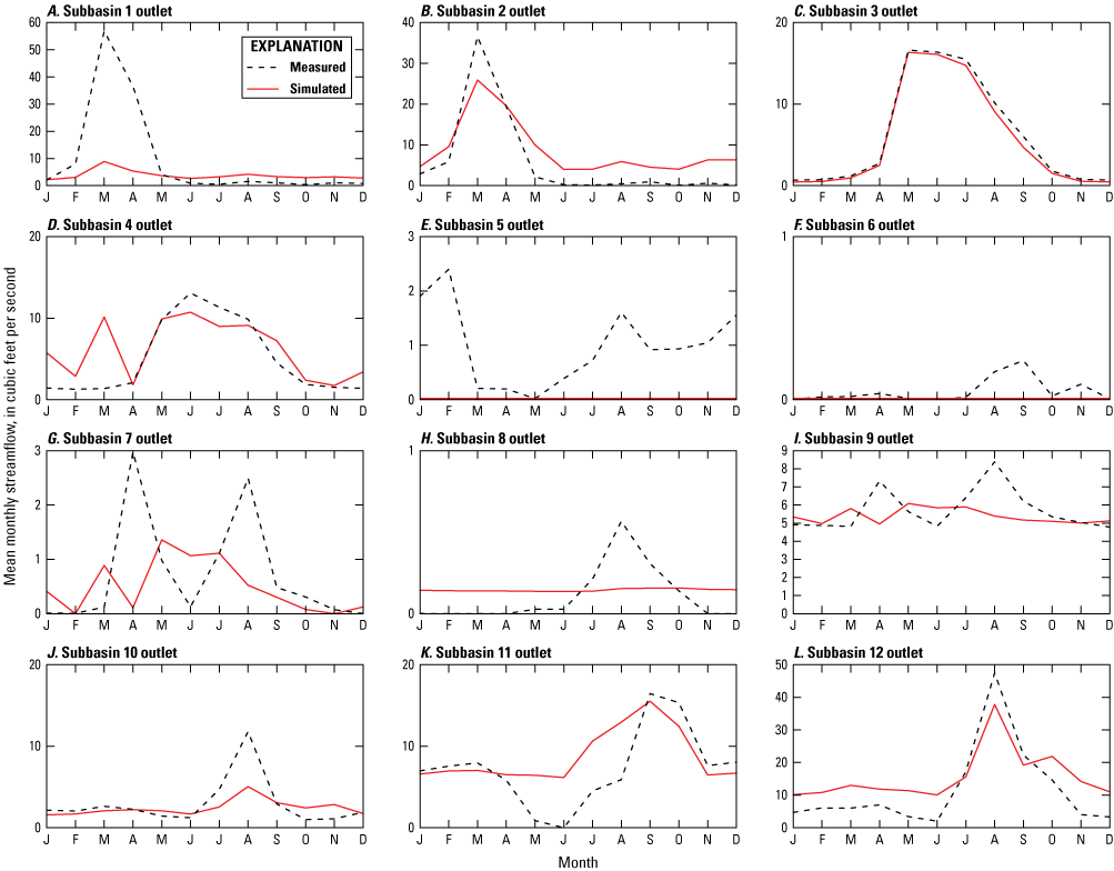
Mean monthly measured streamflow and simulated streamflow at 12 streamgages for the transient MODFLOW-NWT.
Measured mean monthly streamflow at the outlet of subbasin 7, which drains an area extending from the Continental Divide to near the community of Grants (fig. 2), shows a bimodal pattern with pronounced peaks during April and May and July through September (fig. 13). The RSJIHM simulated a bimodal pattern of mean monthly streamflow at the outlet of subbasin 7 that differed from the measured streamflow in the timing and magnitude of the peaks. The RSJIHM simulated a relatively steady mean monthly streamflow at the outlet of subbasin 8, which drains a relatively small area near the community of Grants, that differed from the pronounced measured peak during July through September. Measured mean monthly streamflow at the outlet of subbasin 9 shows a bimodal pattern with pronounced peaks during April and May and July through September. The RSJIHM simulated a bimodal pattern of mean monthly streamflow at the outlet of subbasin 9 that differed from the measured streamflow in the timing and magnitude of the peaks. The RSJIHM simulated the overall patterns of measured mean monthly streamflow at the outlet of subbasin 10, which drains the eastern side of Mount Taylor, with a pronounced peak during July through September, but simulated about half of the maximum measured streamflow peak during August. The RSJIHM was generally able to simulate the bimodal patterns of measured mean monthly streamflow at the outlets of subbasins 11 and 12 near the terminus of the basin, with lower streamflow during May and June and a pronounced peak during July through October.
Monthly Mean
The Nash-Sutcliffe model efficiency coefficient between measured and simulated monthly mean streamflow ranged from −0.37 (“not satisfactory”) at the outlet of subbasin 7 to 0.98 (“very good”) at the outlet of subbasin 3 and was 0.43 (“not satisfactory”) for all streamgages (table 15). The percent bias between measured and simulated monthly mean streamflow ranged from −100 at the outlets of subbasins 5 and 6 to 54 at the outlet of subbasin 2 (both “not satisfactory”) and was 8.7 (“good”) for all streamgages. The R2 between measured and simulated monthly mean streamflow ranged from 0.00010 (“not satisfactory”) at the outlet of subbasin 9 to 0.98 (“very good”) at the outlet of subbasin 3 and was 0.42 (“not satisfactory”) for all streamgages. The R2 could not be calculated at the outlets of subbasins 5 and 6 because simulated monthly mean streamflow was zero. Overall, these quantitative measures indicate spatial variability in the performance of the RSJIHM at simulating measured monthly mean streamflow throughout the active MODFLOW-NWT area.
Annual Mean
The Nash-Sutcliffe model efficiency coefficient between measured and simulated annual mean streamflow ranged from −3.6 (“not satisfactory”) at the outlet of subbasin 6 to 0.99 (“very good”) at the outlet of subbasin 3 and was 0.55 (“satisfactory”) for all streamgages (table 15). The percent bias between measured and simulated annual mean streamflow ranged from −100 at the outlets of subbasins 5 and 6 to 52 at the outlet of subbasin 2 (both “not satisfactory”) and was 7.9 (“good”) for all streamgages. The R2 between measured and simulated annual mean streamflow ranged from 0.00010 (“not satisfactory”) at the outlet of subbasin 9 to 1.0 (“very good”) at the outlet of subbasins 3 and 11 and was 0.58 (“not satisfactory”) for all streamgages. The R2 could not be calculated at the outlets of subbasins 5 and 6 because simulated annual mean streamflow was zero. Overall, these quantitative measures indicate spatial variability in the performance of the RSJIHM at simulating measured annual mean streamflow throughout the active MODFLOW-NWT area.
Hydrographs of measured and simulated annual mean streamflow at the 12 streamgages are shown in fig. 14. In the Zuni uplift, the RSJIHM simulated the overall patterns of measured annual mean streamflow peaks and reductions, with undersimulation of the magnitudes of the peaks at the outlet of subbasin 1 and a mixture of undersimulation and oversimulation of the magnitudes of the peaks at the outlet of subbasin 2. The RSJIHM closely simulated the measured annual mean streamflow at the outlet of subbasin 3. The RSJIHM generally simulated the overall patterns and magnitudes of measured annual mean streamflow at the outlet of subbasin 4, but oversimulated streamflow by greater than 3 ft3/s during 1968, 1971 and 1972. The RSJIHM was unable to simulate the relatively low (less than 2 ft3/s) measured annual mean streamflow at the outlets of subbasins 5 and 6.
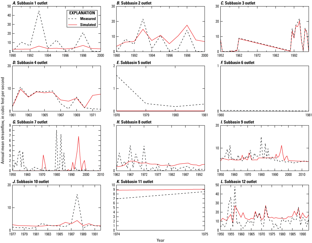
Annual mean of measured daily mean streamflow and simulated daily streamflow at 12 streamgages for the transient MODFLOW-NWT.
The RSJIHM was generally unable to simulate the patterns and magnitudes of measured annual mean streamflow at the outlet of subbasin 7 (fig. 14). The RSJIHM generally simulated the trends of measured annual mean streamflow at the outlet of subbasin 8 but was unable to simulate the peakiness of measured streamflow. The RSJIHM generally simulated the trends of measured annual mean streamflow at the outlet of subbasin 9 but was unable to simulate the magnitudes of the streamflow peaks. At the outlet of subbasin 10, the RSJIHM simulated the overall patterns of measured annual mean streamflow, but only simulated about a quarter of the measured streamflow peak during 1988. The RSJIHM was generally able to simulate the patterns and magnitudes of measured annual mean streamflow at the outlets of subbasins 11 and 12.
During the high precipitation verification year, 1983, the RSJIHM undersimulated measured annual mean streamflow by greater than 6 ft3/s at the outlets of subbasins 7 and 9 (fig. 14). The RSJIHM performed better at simulating measured annual mean streamflow during 1983 at the outlets of subbasins 8, 10, and 12. During the low precipitation verification year, 2018, the RSJIHM oversimulated measured monthly mean streamflow at the outlet of subbasin 9, with the average of the monthly mean streamflow during January through September simulated at 4.1 ft3/s and measured at 3.1 ft3/s. Measured streamflow data were not available at any other streamgages during these verification periods.
Hydraulic Head
The steady-state simulation period of the RSJIHM had an average residual (simulated minus measured head) of −26.17 ft and a median residual of 5.46 ft, and the residuals ranged from about −2,513.44 to 1,776.37 ft, with a standard deviation of 205.71 ft (table 16). The RMSE was 207.34 ft, which represents about 4.0 percent of the 5,149.32-ft range in measured head values. The transient simulation period of the RSJIHM had an average residual of −31.68 ft and a median residual of −5.81 ft, and the residuals ranged from about −2,664.09 to 1,798.31 ft, with a standard deviation of 170.21 ft (table 16). The RMSE was 173.12 ft, which represents about 3.4 percent of the 5,149.32-ft range in measured head values. Table 17 summarizes the median residual by hydrogeologic unit zone that resulted from the calibration of the transient MODFLOW-NWT. These results indicate the accuracy of the RSJIHM at simulating head is spatially variable.
Table 16.
Statistics summarizing the calibration of the steady-state and transient MODFLOW-NWT to measured hydraulic head at 3,561 single and multiple layer wells and 160 spring locations for the Rio San Jose Integrated Hydrologic Model, New Mexico.[RMSE, root mean square error]
Table 17.
Median residuals by hydrogeologic unit zone for the calibration of the transient MODFLOW-NWT to measured hydraulic head at 3,561 single and multiple layer wells and 160 spring locations for the Rio San Jose Integrated Hydrologic Model, New Mexico.[ft2/d, foot squared per day; NA, not applicable]
Correlation graphs of simulated and measured heads for the steady-state and transient simulation periods (figs. 15 and 16, respectively) indicated a generally adequate fit across the wide range of measured heads, as seen by the points generally plotting around the 1:1 line. Overall, the RSJIHM undersimulated measured heads (points below the 1:1 line on figs. 15 and 16), especially at higher measured heads. Most of the highest head measurements above about 8,000 ft are for springs in the Mount Taylor region that emerge as topographic breaks in slope (Langman and others, 2012); these springs are poorly simulated by the RSJIHM. The largest oversimulation of measured heads (points above the 1:1 line on figs. 15 and 16) was found at wells that draw water from the Morrison-Entrada hydrogeologic unit and have a single head measurement obtained from NMOSE POD records. The well with the largest oversimulated head is in the same model grid cell as five other wells that have measured heads at least 2,000 ft greater; thus, the reliability of the head measurement at this well is questionable. Other wells with oversimulated heads could be the result of inaccurate head measurements, incorrect vertical placement in the model, and variations in hydraulic properties not incorporated in the hydrogeologic unit zones.

Correlation graph of simulated against measured hydraulic heads at observation wells and springs for the steady-state MODFLOW-NWT.
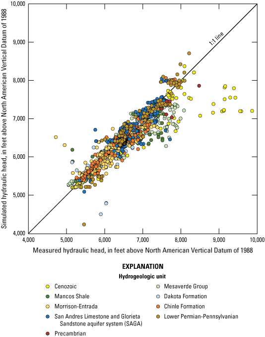
Correlation graph of simulated against measured hydraulic heads at observation wells and springs for the transient MODFLOW-NWT.
The RSJIHM was able to simulate the general patterns of measured head at the six wells within the study area having long-term records of head measurements (table 5 and fig. 17; locations of wells are shown on plate 1). At GRGS14, located in the Cenozoic hydrogeologic unit near Horace Springs, the RSJIHM generally oversimulated measured heads by about 10 ft but matched the relatively steady measured head pattern at this well relative to the other five wells. At URGS9, located in the SAGA hydrogeologic unit near the community of Grants, the RSJIHM undersimulated measured heads by as much as 30 ft but generally matched the measured head pattern at this well including the intra-annual variability in head likely associated with groundwater pumping. At URGS64, located in the Lower Permian-Pennsylvanian hydrogeologic unit near the community of Bluewater, the RSJIHM generally undersimulated measured heads by as much as 180 ft and simulated an increase in head from the 1960s through the 1970s that was not indicated by the measured data. For the 1950s and the 1990s through 2018, the RSJIHM generally simulated the pattern of decreases in head measured at URGS64. At MDGS1, located in the SAGA hydrogeologic unit near the community of Bluewater, the RSJIHM undersimulated measured head values by as much as about 180 ft but generally matched the measured head pattern at this well including the intra-annual variability in head likely associated with groundwater pumping.
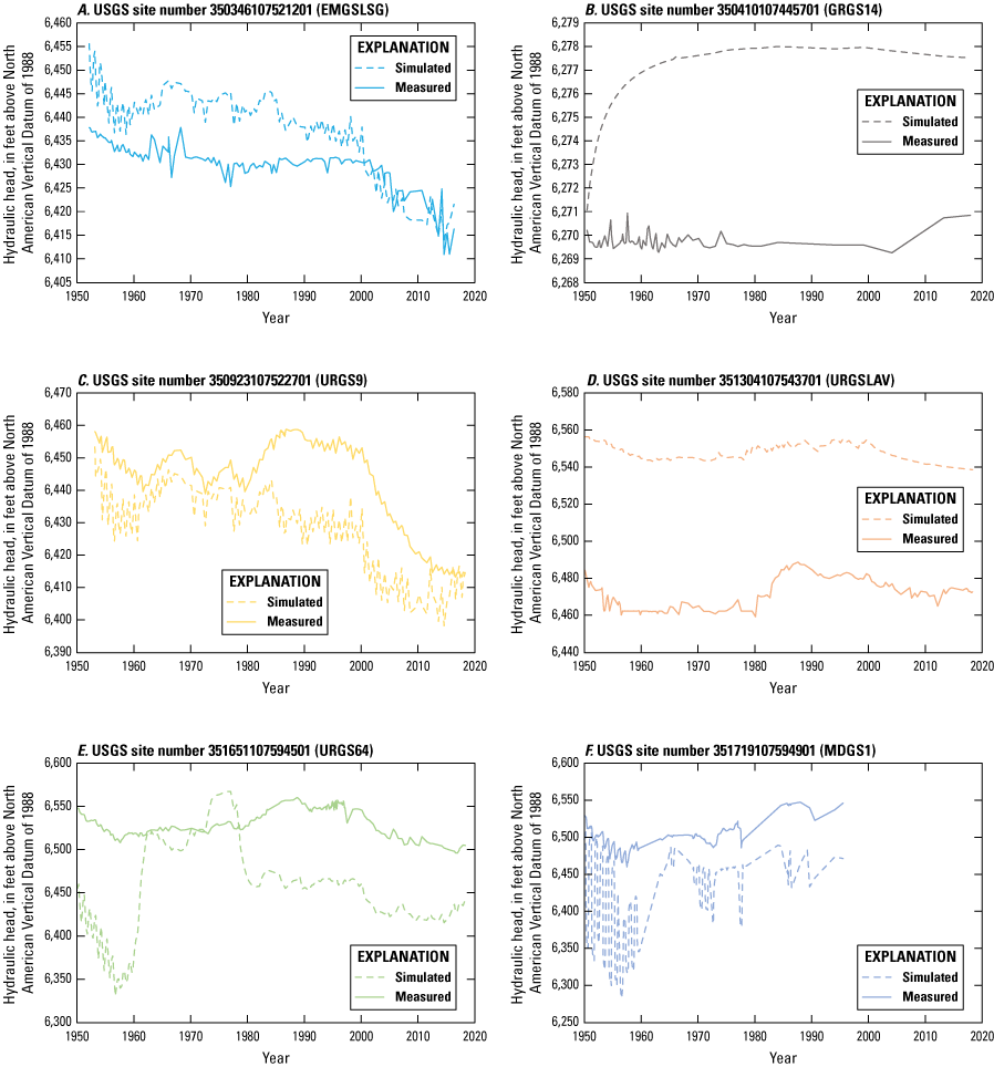
Simulated and measured hydraulic heads at six observation wells with long-term records of hydraulic head measurements that were used for calibration and verification of the transient MODFLOW-NWT. In each hydrograph, the U.S. Geological Survey (USGS) site number is followed by the unique Rio San Jose Integrated Hydrologic Model well identifier in parentheses.
At the two wells used for verification of the transient MODFLOW-NWT (EMGSLSG, located in the SAGA hydrogeologic unit near the community of San Rafael and URGSLAV, located in the Cenozoic hydrogeologic unit near the community of Milan), the RSJIHM generally simulated the measured head patterns but oversimulated measured heads at EMGSLSG by as much as about 20 ft and at URGSLAV by as much as about 80 ft. The verification results suggest the RSJIHM can simulate the hydrologic system response to historical water use and potential changes in water supplies and demands in the study area.
Springflow
The RSJIHM was able to closely simulate (5.1 ft3/s) the average reported springflow at Ojo del Gallo (5 ft3/s) during the steady-state simulation period. During the transient simulation period, the RSJIHM simulated the overall patterns of reported springflow at Ojo del Gallo, including the rapid decline in springflow during the early 1950s, the resurgence in springflow during the early to mid-1980s, and the rapid decline to zero springflow in the late 1980s (fig. 18). However, the RSJIHM undersimulated (maximum simulated springflow of 0.15 ft3/s) the magnitude of the reported springflow resurgence at Ojo del Gallo (1–2 ft3/s) during the early to mid-1980s and simulated periods of springflow resurgence during the 1960s (maximum simulated springflow of 0.29 ft3/s) and 1970s (maximum simulated springflow of 0.18 ft3/s) that were not reported and are assumed to be a period of no springflow.
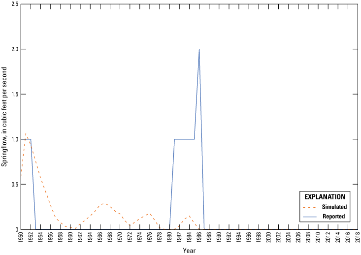
Ojo del Gallo reported springflow and simulated annual mean springflow for the transient MODFLOW-NWT.
The RSJIHM was able to reasonably simulate (4.5 ft3/s) the average estimated springflow at Horace Springs (5.6 ft3/s) during the steady-state simulation period. During the transient simulation period, the RSJIHM undersimulated (4.1 ft3/s) the average estimated annual mean springflow at Horace Springs (4.6 ft3/s), with relatively constant simulated springflow as compared to the temporal variability in estimated springflow (fig. 19). Springflow at Horace Springs was estimated as the daily base flow at Rio San Jose at Acoma, which was estimated using measured daily mean streamflow at this streamgage. The base flow estimates include some fast and intermediate interflow components that can vary seasonally and annually on the basis of climate variability, which may not be representative of the less temporally variable springflow that is likely assuming that groundwater discharge is the predominant water source for Horace Springs.
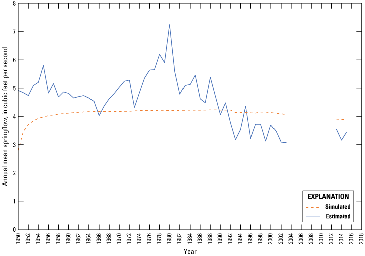
Horace Springs estimated and simulated annual mean springflow for the transient MODFLOW-NWT.
Surface-Water Releases from Bluewater Lake
The RSJIHM was able to closely simulate (7,800 acre-ft) the estimated average annual surface-water release from Bluewater Lake (8,040 acre-ft) during the steady-state simulation period. During the transient simulation period, the RSJIHM simulated the overall patterns of the estimated annual surface-water releases from Bluewater Lake, including the interannual variability, the increase in releases during the 1970s, 1980s, and 1990s, and the decrease in releases during the 2000s and 2010s (fig. 20). However, the RSJIHM generally undersimulated the magnitude of the estimated annual surface-water releases from Bluewater Lake, especially during the 1970s, 1980s, and 1990s.
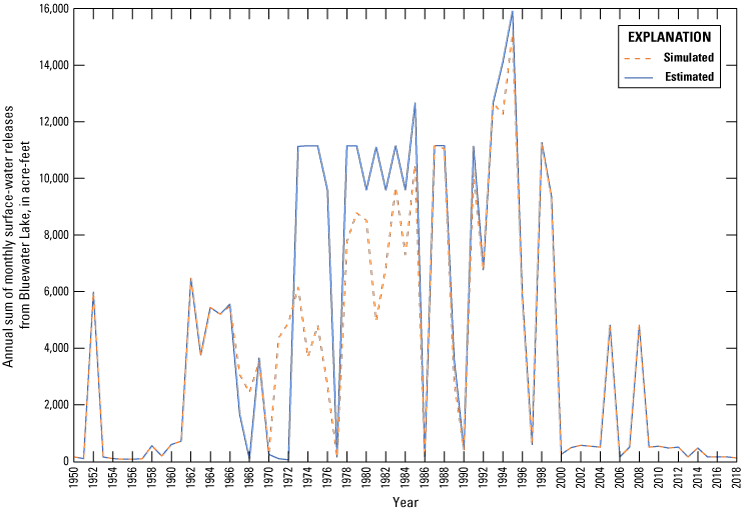
Annual sums of estimated and simulated monthly surface-water releases from Bluewater Lake for the transient MODFLOW-NWT.
Surface-Water Diversions for Irrigation Within the Bluewater-Toltec Irrigation District
The RSJIHM was able to exactly simulate the estimated average annual surface-water diversion for irrigation within the Bluewater-Toltec Irrigation District (2,670 acre-ft) during the steady-state simulation period. During the transient simulation period, the RSJIHM simulated the overall patterns of the estimated annual surface-water diversions for irrigation within the Bluewater-Toltec Irrigation District, including the interannual variability, the increase in diversions during the 1970s and 1980s, and the decrease in diversions during the 2000s and 2010s (fig. 21). However, the RSJIHM undersimulated the magnitude of the estimated annual surface-water diversions for irrigation within the Bluewater-Toltec Irrigation District, with the maximum undersimulation (as much as about 2,500 acre-ft) during the 1970s and 1980s.
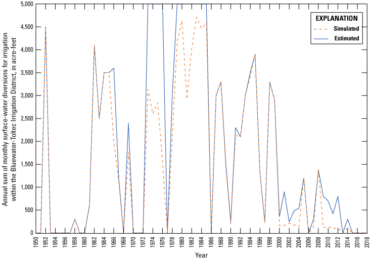
Annual sums of estimated and simulated monthly surface-water diversions for irrigation within the Bluewater-Toltec Irrigation District for the transient MODFLOW-NWT.
Hydrologic Budgets
Hydrologic budgets summarize the magnitude and components of annual simulated flows within the RSJIHM and allow the quantification of the hydrologic system response to the historical evolution of water use in the study area. The average annual PRMS hydrologic budget from 1950 through 2018 indicated the majority (greater than 98 percent) of precipitation within the basin was consumed by evapotranspiration, leaving 1.2 percent to recharge the groundwater system, 0.47 percent to runoff to streams, and 0.20 percent to infiltrate the soil zone and interflow to streams. The higher elevation subbasins 1 and 2 in the Zuni uplift had the greatest average annual percentages of precipitation contributing to groundwater recharge at 4.7 and 11 percent, respectively. Lower elevation subbasins generally had less than 1 percent of precipitation contributing to groundwater recharge, but subbasin 8, which drains a relatively small area near the community of Grants, and subbasin 14, which is a closed subbasin in the southwestern portion of the study area (fig. 2), had relatively large average annual percentages of precipitation contributing to groundwater recharge at 2.1 and 2.9 percent, respectively.
The average annual recharge to the groundwater system simulated by PRMS was about 28,000 acre-ft, with the greatest contributions from subbasin 14 (12,000 acre-ft), subbasin 2 (7,700 acre-ft), and subbasin 1 (3,800 acre-ft). The majority of recharge was associated with snowmelt, with February through April accounting for 61 percent of recharge throughout the active PRMS area and 87 percent of recharge in the higher elevation subbasins 1 and 2 in the Zuni uplift. Few estimates of recharge exist for comparison with the recharge simulated by PRMS. The model of groundwater flow in the Quaternary alluvium and alluvial-basalt sequences, Quaternary basalt aquifers, and the Permian SAGA developed by Frenzel (1992) simulated an average annual recharge of about 8,000 acre-ft, with 3,100 acre-ft of recharge in the Zuni uplift and 4,900 acre-ft of recharge to the basalt flows composing El Malpais National Monument. Frenzel (1992) did not simulate most of the closed subbasin 14 where PRMS simulated 12,000 acre-ft of recharge. Excluding subbasin 14, PRMS simulated about 16,000 acre-ft of recharge in an active area comparable to Frenzel (1992). Summing the average measured annual mean streamflow at the outlet of subbasin 12 near the terminus of the basin (about 8,500 acre-ft), the average reported springflow at Ojo del Gallo (about 3,600 acre-ft), and interbasin groundwater flow to the Middle Rio Grande Basin simulated by McAda and Barroll (2002) (about 1,600 acre-ft) provides an estimate of the steady-state outflow of water from the non-closed portion of the basin at about 14,000 acre-ft, which is comparable to the 16,000 acre-ft of recharge simulated by PRMS.
The average annual runoff to streams simulated by PRMS was about 11,000 acre-ft, with the greatest contributions from subbasin 12 (2,700 acre-ft), subbasin 14 (2,400 acre-ft), and subbasin 2 (1,800 acre-ft). The majority of runoff to streams was associated with the summer monsoon, with May through October accounting for 65 percent of runoff throughout the active PRMS area. The average annual soil zone interflow to streams simulated by PRMS was about 4,500 acre-ft, with the greatest contributions from subbasin 14 (2,100 acre-ft), subbasin 12 (1,400 acre-ft), and subbasin 1 (250 acre-ft).
The annual MODFLOW-NWT hydrologic budget for the steady-state simulation period of the RSJIHM resulted in the following outflows from the groundwater system:
-
1,300 acre-ft of groundwater pumping;
-
1,600 acre-ft of interbasin groundwater flow to the Middle Rio Grande Basin;
-
25,000 acre-ft of groundwater discharge to streams and springs;
-
1.1 acre-ft of seepage to Bluewater Lake; and
-
28,000 acre-ft of recharge as inflow to the groundwater system.
The annual MODFLOW-NWT hydrologic budget for the transient simulation period of the RSJIHM is presented in fig. 22. For the line indicating cumulative aquifer storage change, a negative slope indicates depletion of aquifer storage and a positive slope indicates accretion of aquifer storage.
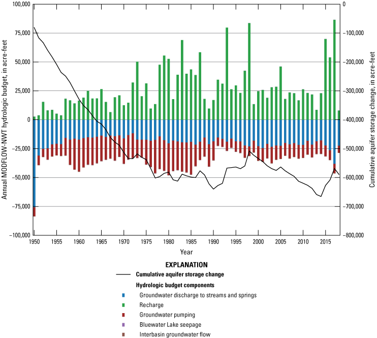
Simulated annual MODFLOW-NWT hydrologic budget, 1950 through 2018, and cumulative aquifer storage change for the Rio San Jose Integrated Hydrologic Model, New Mexico. Budget components contributing to an outflow from the groundwater system are plotted below zero and budget components contributing to an inflow to the groundwater system are plotted above zero.
During the 1950s through the late 1970s, the RSJIHM generally simulated aquifer storage depletion (fig. 22). The decline corresponds to the expansion of groundwater pumping (indicated by withdrawals increasing from 13,000 to 30,000 acre-ft/yr) in the study area to meet the demands of the mining industry and subsequent municipal development. For the 1980s through the late 1990s, the RSJIHM simulated an overall pattern of aquifer storage accretion. During this period, most of the aquifer storage accretion happened during years with increased recharge simulated by PRMS and declining groundwater pumping (indicated by withdrawals decreasing from 30,000 to 13,000 acre-ft/yr) associated with the cessation of mining activities in the 1980s. For the late 1990s through 2014, the RSJIHM generally simulated aquifer storage depletion with steady groundwater pumping (indicated by withdrawals averaging 15,000 acre-ft/yr) and decreased recharge as compared to the wetter period of the 1980s to the late 1990s. For 2015 through 2017, increased recharge simulated by PRMS, mostly in the closed subbasin (subbasin 14 on fig. 2) in the southwestern portion of the study area, resulted in aquifer storage accumulation. Overall, the RSJIHM simulated about 590,000 acre-ft of cumulative aquifer storage depletion from 1950 through 2018.
The simulated annual groundwater pumping (outflow from the groundwater system) and deep percolation, injection, and seepage (inflow to the groundwater system) by hydrogeologic unit are presented on fig. 23. During the 1950s through the early 1980s, most groundwater pumping was from the Morrison-Entrada hydrogeologic unit and was associated with dewatering activities of the mining industry. The SAGA and Cenozoic hydrogeologic units have been consistent sources of water for municipal use in the study area, with withdrawals from the SAGA peaking at about 13,000 acre-ft in 2003. Deep percolation to the Cenozoic hydrogeologic unit represents the primary source of inflow to the groundwater system.
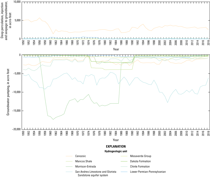
Simulated annual MODFLOW-NWT groundwater pumping (outflow from the groundwater system) and deep percolation, injection, and seepage (inflow to the groundwater system) by hydrogeologic unit for the Rio San Jose Integrated Hydrologic Model, New Mexico.
Groundwater discharge to streams and springs generally decreased during the 1950s through the late 1970s, corresponding to increased groundwater pumping (fig. 22). After the cessation of mining activities in the 1980s, groundwater discharge to streams and springs generally increased. Seepage to and from Bluewater Lake represented the smallest component of the MODFLOW-NWT hydrologic budget, averaging less than 1 acre-ft/yr, and was within the uncertainty generated by the mass balance errors of MODFLOW-NWT (see “Mass Balance” section).
Interbasin groundwater flow across the western, northern, and eastern boundaries of MODFLOW-NWT represented a small, but generally steady, component of the hydrologic budget, averaging about 410 acre-ft/yr (standard deviation of 47 acre-ft/yr) of groundwater flow out of the active area with most exiting across the boundary with the Middle Rio Grande Basin. McAda and Barroll (2002) simulated approximately 1,600 acre-ft/yr of groundwater flow into the Middle Rio Grande Basin across the boundary with the RSJIHM from 1900 through 2000. An average of less than 1 acre-ft/yr was simulated to leave the active area along the western and northern boundaries of the RSJIHM.
Model Limitations and Uncertainty, and Data Needs for Model Enhancement
The RSJIHM, like all models, is a simplification of the complex natural hydrologic system. The ability of the RSJIHM to simulate the natural hydrologic system is controlled by factors such as the spatial and temporal discretization of the model, model layering and hydraulic property distribution, the accuracy of the spatial and temporal distribution of data incorporated in the model, and the availability and accuracy of historical data used for model calibration. The RSJIHM uses a constant-area horizontal grid discretization of 0.25 square kilometer and will not provide an accurate simulation of the hydrologic system at a scale less than this horizontal discretization. The RSJIHM is appropriate to simulate the local scale (tens of square miles) to regional scale (thousands of square miles) response of the Rio San Jose Basin hydrologic system at temporal resolutions of months to years. For example, the RSJIHM can be used to simulate the impacts of anticipated groundwater pumping to streamflow and groundwater levels in nearby wells.
PRMS simulated relatively large recharge to the groundwater system and runoff and soil zone interflow to streams in subbasin 14, which is a closed subbasin (fig. 2) in the southwestern portion of the study area. Subbasin 14 is in a remote portion of the study area, and only two measured or estimated datasets (solar radiation and potential evapotranspiration) were available for calibration of the parameters in this subbasin. Thus, parameters and simulated results from the RSJIHM should be considered uncertain in and within the vicinity of subbasin 14. The RSJIHM could benefit from additional data collection (streamflow, head, springflow) in this remote area to verify and improve the simulation of the RSJIHM.
The RSJIHM was unable to simulate the pronounced peak in measured mean monthly streamflow during March and April at the outlet of subbasin 1. The RSJIHM did a much better job of simulating the peak in streamflow at the outlet of subbasin 2, but still undersimulated the peak streamflow. These results indicate the RSJIHM is lacking in its simulation of hydrologic processes in the higher elevation subbasins in the Zuni uplift. The RSJIHM could benefit from additional data collection (precipitation, evapotranspiration, streamflow, head, springflow) in this area to verify and improve the simulation of the RSJIHM. In subbasins where the RSJIHM performed “unsatisfactory” at simulating measured streamflow, results of simulations to assess the impacts to streamflow from changes to hydrologic stresses should be considered uncertain.
The RSJIHM could benefit from the incorporation of temporal variability in vegetation cover and type within PRMS. The RSJIHM used a snapshot in time from the LANDFIRE 2014 (lf_1.4.0) datasets to generate parameters related to vegetation. Thus, the RSJIHM assumed constant vegetation cover and type within the study area. Additional work with the RSJIHM that includes temporally variable vegetation parameters could improve model simulation capability for historical or future periods.
The daily climate inputs (precipitation and minimum and maximum air temperature) to PRMS were extracted from gridded, hydrometeorological datasets (Livneh and others, 2015; Thornton and others, 2016) at the centroid of each HRU. These Livneh and others (2015) and Daymet hydrometeorological datasets were gridded at horizontal resolutions of 6 and 1 km, respectively, whereas the RSJIHM was gridded at a horizontal resolution of 500 m. The RSJIHM could benefit from the spatial downscaling of the hydrometeorological datasets to model the spatial variability of the climate inputs at the scale of the study area. Additional work with the RSJIHM may consider spatial downscaling of hydrometeorological datasets used for historical or future periods.
The RSJIHM could benefit from the incorporation of more spatial variability in hydraulic properties within hydrogeologic units, especially in the hydrogeologic units that were represented with a single hydrogeologic unit zone. Additional work with the RSJIHM may consider calibrating parameter values at pilot point locations to add spatial variability to hydraulic property parameters that could improve the simulation capability of the RSJIHM. The calibration of hydraulic property parameter values at pilot point locations would benefit from additional data collection, such as aquifer tests and geophysics, that could provide constraints to the spatial variability of hydraulic properties within hydrogeologic units that have scarce hydraulic property data.
The RSJIHM was calibrated to a wide range of datasets covering the study area from the plant canopy to the land surface, soil zone, streams and lakes, and saturated subsurface zone. However, as new data become available, the model should be periodically updated to verify the simulation capability and possibly revise the parameterization determined in this study. Geochemical data, in particular environmental tracers such as carbon-14, tritium, deuterium, and oxygen-18, are an example of additional data that could be useful to incorporate into the RSJIHM to verify the spatial distribution and rates of recharge, groundwater flow paths, and groundwater residence times.
Summary
The Rio San Jose Integrated Hydrologic Model (RSJIHM) was developed to provide a tool for analyzing the hydrologic system response to historical water use and potential changes in water supplies and demands in the Rio San Jose Basin. The study area encompasses about 6,300 square miles in west-central New Mexico and includes the communities of Grants, Bluewater, and San Rafael and three Native American Tribal lands: the Acoma and Laguna Pueblos and the Navajo Nation. Perennial surface water features are sparse in the study area and most water resources consist of groundwater pumped from sedimentary and basalt aquifers. The RSJIHM is an integration of the U.S. Geological Survey Precipitation-Runoff Modeling System (PRMS) and MODFLOW-NWT and provides a tool to help support long-term planning and management decisions regarding the basin’s surface-water and groundwater resources.
Calibration of PRMS was performed using PEST++ (version 4.3.20), and the parameters that were adjusted during calibration were those that control the (1) solar radiation; (2) potential evapotranspiration distribution; (3) evapotranspiration and sublimation; (4) air temperature and precipitation distribution; (5) streamflow; (6) Hortonian surface runoff, infiltration, and impervious storage; (7) interception; (8) soil zone storage, interflow, gravity drainage, and Dunnian surface runoff; (9) groundwater flow; and (10) snow computations. Adjustments to PRMS parameter values during calibration were based on the ability of model simulated values to reproduce measured or estimated values for several observation groups: (1) solar radiation, (2) potential evapotranspiration, (3) actual evapotranspiration, (4) precipitation and minimum and maximum air temperature, (5) snow water equivalent, (6) snow-covered area, and (7) streamflow. Calibration of MODFLOW-NWT was performed using BeoPEST (version 13.6) and the parameters that were adjusted during calibration were horizontal hydraulic conductivity, vertical anisotropy, specific yield, and specific storage of model layers; hydraulic conductance within the General-Head Boundary package; hydraulic characteristic within the Horizontal Flow Barrier package; hydraulic conductivity of the streambed and springbed; elevation of the top of the streambed and springbed; and lakebed leakance. Adjustments to MODFLOW-NWT parameter values during calibration were based on the ability of model simulated values to reproduce measured, estimated, or reported values for several observation groups: (1) streamflow, (2) hydraulic head, (3) springflow at Ojo del Gallo, (4) springflow at Horace Springs, (5) surface-water releases from Bluewater Lake, and (6) surface-water diversions for irrigation within the Bluewater-Toltec Irrigation District.
The MODFLOW-NWT mass balance errors represented a small fraction of the total inflows and outflows (annual absolute volume errors represented a maximum of 0.74 percent of annual total inflows or outflows) simulated by the RSJIHM, and the results for most hydrologic budget components were greater than the uncertainty generated by these errors. Overall, the RSJIHM demonstrates a robust ability to simulate the spatially and temporally variable measurements, estimates, or reports of the hydrologic system state, with low mass balance errors.
The simulated average annual PRMS hydrologic budget from 1950 through 2018 indicated the majority (greater than 98 percent) of precipitation within the basin was consumed by evapotranspiration, leaving 1.2 percent to recharge the groundwater system, 0.47 percent to runoff to streams, and 0.20 percent to infiltrate the soil zone and interflow to streams. The higher elevation subbasins 1 and 2 in the Zuni uplift had the greatest average annual percentages of precipitation contributing to groundwater recharge at 4.7 and 11 percent, respectively. Lower elevation subbasins generally had less than 1 percent of precipitation contributing to groundwater recharge. The average annual recharge to the groundwater system and runoff to streams simulated by the RSJIHM was about 28,000 and 11,000 acre-feet, respectively. The majority of recharge was associated with snowmelt, with February through April accounting for 61 percent of recharge throughout the active PRMS area and 87 percent of recharge in the higher elevation subbasins 1 and 2 in the Zuni uplift. The majority of runoff to streams was associated with the summer monsoon, with May through October accounting for 65 percent of runoff throughout the active PRMS area.
Overall, the RSJIHM simulated about 590,000 acre-feet of cumulative aquifer storage depletion from 1950 through 2018. Groundwater discharge to streams and springs generally decreased during the 1950s through the late 1970s, corresponding to increased groundwater pumping, and generally increased after the cessation of mining activities in the 1980s. Interbasin groundwater flow across the western, northern, and eastern boundaries of the RSJIHM represented a small, but generally stable, component of the MODFLOW-NWT hydrologic budget, averaging about 410 acre-feet per year (standard deviation of 47 acre-feet per year) of groundwater flow out of the active area from 1950 through 2018.
The RSJIHM is a simplification of the complex natural hydrologic system and is appropriate to simulate the local scale (tens of square miles) to the regional scale (thousands of square miles) response of the Rio San Jose Basin hydrologic system at temporal resolutions of months to years. The RSJIHM could benefit from additional data collection (streamflow, head, springflow) in the southwestern subbasin that includes the El Malpais National Monument to verify and improve the simulation capability of the RSJIHM in a substantially large portion of the active area. Additional work that could improve the simulation capability of the RSJIHM includes incorporating temporally variable vegetation parameters, spatial downscaling of the hydrometeorological input datasets, incorporating additional spatial variability to hydraulic property parameters on the basis of new data collection, and using environmental tracers to verify and calibrate model parameters.
References Cited
Arcement, G.J., Jr., and Schneider, V.R., 1989, Guide for selecting Manning’s roughness coefficients for natural channels and flood plains: U.S. Geological Survey Water Supply Paper 2339, 38 p., accessed January 31, 2023, at https://doi.org/10.3133/wsp2339.
Bakker, M., Post, V., Langevin, C.D., Hughes, J.D., White, J.T., Starn, J.J., and Fienen, M.N., 2016, Scripting MODFLOW model development using Python and FloPy: Ground Water, v. 54, no. 5, p. 733–739, accessed January 31, 2023, at https://doi.org/10.1111/gwat.12413.
Baldwin, J.A., and Anderholm, S.K., 1992, Hydrogeology and ground-water chemistry of the San Andres-Glorieta aquifer in the Acoma embayment and eastern Zuni uplift, west-central New Mexico: U.S. Geological Survey Water-Resources Investigations Report 91–4033, 304 p., accessed September 12, 2019, at https://doi.org/10.3133/wri914033.
Baldwin, J.A., and Rankin, D.R., 1995, Hydrogeology of Cibola County, New Mexico: U.S. Geological Survey Water-Resources Investigations Report 94–4178, 102 p., accessed January 28, 2020, at https://doi.org/10.3133/wri944178.
Barlow, P.M., Cunningham, W.L., Zhai, T., and Gray, M., 2015, U.S. Geological Survey groundwater toolbox, a graphical and mapping interface for analysis of hydrologic data (version 1.0)—User guide for estimation of base flow, runoff, and groundwater recharge from streamflow data: U.S. Geological Survey Techniques and Methods, book 3, chap. B10, 27 p., accessed April 8, 2022, at https://doi.org/10.3133/tm3B10.
Beaumont, E.C., 1987, Geology and mining activity in the Lee Ranch area, McKinley County, New Mexico, in Roybal, G.H., Anderson, O.J., and Beaumont, E.C., eds., Coal deposits and facies changes along the southwestern margin of the Late Cretaceous seaway, west-central New Mexico: New Mexico Bureau of Mines & Mineral Resources Bulletin 121, p. 37–40.
Blodgett, D.L., Booth, N.L., Kunicki, T.C., Walker, J.L., and Viger, R.J., 2011, Description and testing of the Geo Data Portal—Data integration framework and Web processing services for environmental science collaboration: U.S. Geological Survey Open-File Report 2011–1157, 9 p., accessed March 8, 2022, at https://pubs.usgs.gov/of/2011/1157/.
Chavarria, S.B., Moeser, C.D., and Douglas-Mankin, K.R., 2020, Application of the Precipitation-Runoff Modeling System (PRMS) to simulate near-native streamflow in the Upper Rio Grande Basin: U.S. Geological Survey Scientific Investigations Report 2020–5026, 38 p., accessed March 9, 2022, at https://doi.org/10.3133/sir20205026.
DeCicco, L., Hirsch, R., Lorenz, D., Read, J., Walker, J., Carr, L., Watkins, D., Blodgett, D., and Johnson, M., 2022, Package ‘dataRetrieval’: Comprehensive R Archive Network (CRAN), accessed March 8, 2022, at https://cran.r-project.org/web/packages/dataRetrieval/dataRetrieval.pdf.
Esri, 2018, MODIS Toolbox—A toolbox to help you import data from MODIS: Toolbox by Esri, accessed March 8, 2022, at https://hydroteam.maps.arcgis.com/home/item.html?id=5fe74de4ec254bc09515e562abe994e1.
Esri, 2020, World terrain base: Tile layer by Esri, accessed March 4, 2022, at https://server.arcgisonline.com/ArcGIS/rest/services/World_Terrain_Base/MapServer.
Esri, 2022, Tabulate intersection (analysis): Tool by Esri, accessed March 8, 2022, at https://pro.arcgis.com/en/pro-app/2.8/tool-reference/analysis/tabulate-intersection.htm.
Fenneman, N.M., and Johnson, D.W., 1946, Physical divisions of the United States: U.S. Geological Survey, 1 plate, accessed December 31, 2019, at https://doi.org/10.3133/70207506.
Frenzel, P.F., 1992, Simulation of ground-water flow in the San Andres-Glorieta aquifer in the Acoma embayment and eastern Zuni uplift, west-central New Mexico: U.S. Geological Survey Water-Resources Investigations Report 91–4099, 381 p., accessed December 31, 2019, at https://doi.org/10.3133/wri914099.
Frenzel, P.F., and Lyford, F.P., 1982, Estimates of vertical hydraulic conductivity and regional ground-water flow rates in rocks of Jurassic and Cretaceous age, San Juan Basin, New Mexico and Colorado: U.S. Geological Survey Water-Resources Investigations Report 82–4015, 59 p., accessed January 31, 2020, at https://doi.org/10.3133/wri824015.
GeoPandas Developers, 2022, API reference: GeoPandas, accessed May 11, 2022, at https://geopandas.org/en/stable/docs/reference.html.
Hall, D.K., and Riggs, G.A., 2016, MODIS/Terra snow cover daily L3 global 500m SIN grid, version 6: National Aeronautics and Space Administration National Snow and Ice Data Center Distributed Active Archive Center, accessed November 14, 2020, at https://doi.org/10.5067/MODIS/MOD10A1.006.
Harbaugh, A.W., 2005, MODFLOW-2005, the U.S. Geological Survey modular ground-water model—The Ground-Water Flow Process: U.S. Geological Survey Techniques and Methods, book 6, chap. A16, accessed January 31, 2023, at https://doi.org/10.3133/tm6A16.
Harmel, R.D., Baffaut, C., and Douglas-Mankin, K., 2018, Review and development of ASABE Engineering Practice 621—Guidelines for calibrating, validating, and evaluating hydrologic and water quality models: Transactions of the ASABE, v. 61, no. 4, p. 1393–1401, accessed February 10, 2020, at https://doi.org/10.13031/trans.12806.
Harmel, R.D., Smith, P.K., Migliaccio, K.W., Chaubey, I., Douglas-Mankin, K.R., Benham, B., Shukla, S., Muñoz-Carpena, R., and Robson, B.J., 2014, Evaluating, interpreting, and communicating performance of hydrologic/water quality models considering intended use—A review and recommendations: Environmental Modelling & Software, v. 57, p. 40–51, accessed February 10, 2020, at https://doi.org/10.1016/j.envsoft.2014.02.013.
Henson, W.R., Medina, R.L., Mayers, C.J., Niswonger, R.G., and Regan, R.S., 2013, CRT—Cascade Routing Tool to define and visualize flow paths for grid-based watershed models: U.S. Geological Survey Techniques and Methods, book 6, chap. D2, 28 p., accessed January 31, 2023, at https://doi.org/10.3133/tm6D2.
Hill, M.C., Banta, E.R., Harbaugh, A.W., and Anderman, E.R., 2000, MODFLOW-2000, the U.S. Geological Survey modular ground-water model—User guide to the Observation, Sensitivity, and Parameter-Estimation Processes and three post-processing programs: U.S. Geological Survey Open-File Report 00–184, 210 p.
Homestake Mining Company of California and Hydro-Engineering, LLC, 2004, 2003 annual monitoring report/performance review for Homestake’s Grants project pursuant to NRC license SUA-1471 and discharge plan DP-200: U.S. Nuclear Regulatory Commission and New Mexico Environment Department, prepared by Homestake Mining Company and Hydro-Engineering, LLC, 316 p.
Homestake Mining Company of California and Hydro-Engineering, LLC, 2009, 2008 annual monitoring report/performance review for Homestake’s Grants project pursuant to NRC license SUA-1471 and discharge plan DP-200: U.S. Nuclear Regulatory Commission and New Mexico Environment Department, prepared by Homestake Mining Company and Hydro-Engineering, LLC, 273 p.
Homestake Mining Company of California and Hydro-Engineering, LLC, 2013, 2012 annual monitoring report/performance review for Homestake’s Grants project pursuant to NRC license SUA-1471 and discharge plan DP-200: U.S. Nuclear Regulatory Commission and New Mexico Environment Department, prepared by Homestake Mining Company of California and Hydro-Engineering, LLC, 522 p.
Homestake Mining Company of California and Hydro-Engineering, LLC, 2014, 2013 annual monitoring report/performance review for Homestake’s Grants project pursuant to NRC license SUA-1471 and discharge plan DP-200: U.S. Nuclear Regulatory Commission and New Mexico Environment Department, prepared by Homestake Mining Company of California and Hydro-Engineering, LLC, 550 p.
Homestake Mining Company of California and Hydro-Engineering, LLC, 2016, 2015 annual monitoring report/performance review for Homestake’s Grants project pursuant to NRC license SUA-1471 and discharge plan DP-200: U.S. Nuclear Regulatory Commission and New Mexico Environment Department, prepared by Homestake Mining Company of California and Hydro-Engineering, LLC, 706 p.
Hudson, M.R., and Grauch, V.J.S., 2013, Introduction, in Hudson, M.R., and Grauch, V.J.S., eds., New perspectives on Rio Grande Rift basins—From tectonics to groundwater: Geological Society of America Special Paper 494, p. v–xii, accessed December 10, 2019, at https://doi.org/10.1130/2013.2494(00).
Kernodle, J.M., 1996, Hydrogeology and steady-state simulation of ground-water flow in the San Juan Basin, New Mexico, Colorado, Arizona, and Utah: U.S. Geological Survey Water-Resources Investigations Report 95–4187, 117 p., accessed January 31, 2020, at https://doi.org/10.3133/wri954187.
Langman, J.B., Sprague, J.E., and Durall, R.A., 2012, Geologic framework, regional aquifer properties (1940s–2009), and spring, creek, and seep properties (2009–10) of the upper San Mateo Creek Basin near Mount Taylor, New Mexico: U.S. Geological Survey Scientific Investigations Report 2012–5019, 96 p.
Lawrimore, J.H., Menne, M.J., Gleason, B.E., Williams, C.N., Wuertz, D.B., Vose, R.S., and Rennie, J., 2011, Global Historical Climatology Network—Monthly (GHCN-M), Version 3: National Oceanic and Atmospheric Administration National Centers for Environmental Information, accessed March 10, 2022, at https://doi.org/10.7289/V5X34VDR.
Livneh, B., Bohn, T.J., Pierce, D.W., Munoz-Arriola, F., Nijssen, B., Vose, R., Cayan, D.R., and Brekke, L., 2015, A spatially comprehensive, hydrometeorological data set for Mexico, the U.S., and Southern Canada 1950–2013: Scientific Data, v. 2, accessed October 20, 2020, at https://doi.org/10.1038/sdata.2015.42.
Lorenzo, F., and Watchempino, L., 2003, Acoma Pueblo takes a unique approach to water planning, in New Mexico water planning 2003—48th Annual New Mexico Water Conference Proceedings: Water Resources Research Institute Report, no. 329, p. 43–50, accessed February 27, 2020, at https://nmwrri.nmsu.edu/wp-content/uploads/2015/watcon/proc48/lorenzo-watchempino.pdf.
Magnuson, M.L., Valdez, J.M., Lawler, C.R., Nelson, M., and Petronis, L., 2019, New Mexico water use by categories 2015: New Mexico Office of the State Engineer Technical Report 55, 142 p., accessed September 23, 2022, at https://www.ose.state.nm.us/WUC/wuc_waterUseData.php.
Mankin, K.R., Rumsey, C., Sexstone, G., Ivahnenko, T., Houston, N., Chavarria, S., Senay, G., Foster, L., Thomas, J., Flickinger, A., Galanter, A.E., Moeser, C.D., Welborn, T.L., Pedraza, D.E., Lambert, P.M., and Johnson, M.S., 2022, Upper Rio Grande Basin water-resource status and trends, focus area study review and synthesis: Journal of the American Society of Agricultural and Biological Engineers, v. 65, no. 4, p. 881–901, accessed February 2, 2023 at https://doi.org/10.13031/ja.14964.
Markstrom, S.L., Niswonger, R.G., Regan, R.S., Prudic, D.E., and Barlow, P.M., 2008, GSFLOW—Coupled ground-water and surface-water flow model based on the integration of the Precipitation-Runoff Modeling System (PRMS) and the Modular Ground-Water Flow Model (MODFLOW-2005): U.S. Geological Survey Techniques and Methods, book 6, chap. D1, 240 p.
Markstrom, S.L., Regan, R.S., Hay, L.E., Viger, R.J., Webb, R.M.T., Payn, R.A., and LaFontaine, J.H., 2015, PRMS-IV, the Precipitation-Runoff Modeling System, Version 4: U.S. Geological Survey Techniques and Methods, book 6, chap. B7, 158 p., accessed March 3, 2022, at https://doi.org/10.3133/tm6B7.
McAda, D.P., and Barroll, P., 2002, Simulation of ground-water flow in the Middle Rio Grande Basin between Cochiti and San Acacia, New Mexico: U.S. Geological Survey Water-Resources Investigations Report 02–4200, 81 p., accessed October 23, 2018, at https://doi.org/10.3133/wri20024200.
McDonald, M.G., and Harbaugh, A.W., 1988, A modular three-dimensional finite-difference ground-water flow model: U.S. Geological Survey Techniques of Water-Resources Investigations, book 6, chap. A1, 586 p., accessed September 15, 2022, at https://doi.org/10.3133/twri06A1.
McLaughlin, D., and Johnson, W.K., 1987, Comparison of three groundwater modeling studies: Journal of Water Resources Planning and Management, v. 113, no. 3, p. 405–421, accessed January 31, 2023, at https://doi.org/10.1061/(ASCE)0733-9496(1987)113:3(405).
Merritt, M.L., and Konikow, L.F., 2000, Documentation of a computer program to simulate lake-aquifer interaction using the MODFLOW ground water flow model and the MOC3D solute-transport model: U.S. Geological Survey Water-Resources Investigations Report 2000–4167, 146 p., accessed March 2, 2020, at https://doi.org/10.3133/wri004167.
National Academies of Sciences, Engineering, and Medicine, 2016, Nutrient requirements of beef cattle (8th ed): Washington, D.C., The National Academies Press, 494 p., accessed January 31, 2023, at https://doi.org/10.17226/19014.
National Oceanic and Atmospheric Administration, 2018, Data Tools—Find a station: National Oceanic and Atmospheric Administration website, accessed May 22, 2018, at https://www.ncdc.noaa.gov/cdo-web/datatools/findstation.
National Resources Conservation Service, 2022, Rice Park (933)—Site information and reports: National Resources Conservation Service National Water and Climate Center, accessed May 11, 2022, at https://wcc.sc.egov.usda.gov/nwcc/site?sitenum=933.
New Mexico Bureau of Geology and Mineral Resources, 2019, New Mexico Bureau of Geology and Mineral Resources Interactive Map: accessed June 18, 2018, at https://maps.nmt.edu/.
New Mexico Energy, Minerals, and Natural Resources Department, 2022, Bluewater Lake State Park boating: New Mexico Energy, Minerals, and Natural Resources Department website accessed March 7, 2022, at https://www.emnrd.nm.gov/spd/find-a-park/bluewater-lake-state-park/bluewater-lake-state-park-boating/.
New Mexico Office of the State Engineer [NMOSE], 2018, OSE Points of Diversion shapefile: New Mexico Office of the State Engineer database accessed October 2, 2018, at http://geospatialdata-ose.opendata.arcgis.com/datasets/ose-points-of-diversion.
New Mexico Office of the State Engineer [NMOSE], 2019, New Mexico Water Rights Reporting System: New Mexico Office of the State Engineer, accessed October 4, 2018, at http://nmwrrs.ose.state.nm.us/nmwrrs/index.html.
Niswonger, R.G., Panday, S., and Ibaraki, M., 2011, MODFLOW-NWT, A Newton formulation for MODFLOW-2005: U.S. Geological Survey Techniques and Methods, book 6, chap. A37, 44 p., accessed January 31, 2023, at https://doi.org/10.3133/tm6A37.
Plummer, L.N., Bexfield, L.M., Anderholm, S.K., Sanford, W.E., and Busenberg, E., 2012, Geochemical characterization of ground-water flow in the Santa Fe Group aquifer system, Middle Rio Grande Basin, New Mexico (ver. 1.2, November 20, 2012): U.S. Geological Survey Water-Resources Investigations Report 03–4131, 395 p., CD-ROM in pocket. [Also available at https://pubs.usgs.gov/wri/wri034131/.]
Posson, D.R., Hearne, G.A., Tracy, J.V., and Frenzel, P.F., 1980, A computer program for simulating geohydrologic systems in three dimensions: U.S. Geological Survey Open-File Report 80–421, 806 p., accessed September 15, 2022, at https://doi.org/10.3133/ofr80421.
Precipitation Runoff on Independent Slopes Model Climate Group, 2015, 30-year normals—1981–2010: Oregon State University, accessed February 5, 2020, at http://prism.oregonstate.edu/normals/.
R Core Team, 2022, R—The R project for statistical computing: Vienna, Austria, R Foundation for Statistical Computing, accessed March 8, 2022, at https://www.r-project.org/.
Regan, R.S., and LaFontaine, J.H., 2017, Documentation of the dynamic parameter, water-use, stream and lake flow routing, and two summary output modules and updates to surface-depression storage simulation and initial conditions specification options with the Precipitation-Runoff Modeling System (PRMS): U.S. Geological Survey Techniques and Methods, book 6, chap. B8, 60 p., accessed March 8, 2022, at https://doi.org/10.3133/tm6B8.
Regan, R.S., Juracek, K.E., Hay, L.E., Markstrom, S.L., Viger, R.J., Driscoll, J.M., LaFontaine, J.H., and Norton, P.A., 2019, The U.S. Geological Survey National Hydrologic Model infrastructure—Rationale, description, and application of a watershed-scale model for the conterminous United States: Environmental Modelling & Software, v. 111, p. 192–203, accessed March 9, 2022, at https://doi.org/10.1016/j.envsoft.2018.09.023.
Regan, R.S., Markstrom, S.L., Hay, L.E., Viger, R.J., Norton, P.A., Driscoll, J.M., LaFontaine, J.H., 2018, Description of the National Hydrologic Model for use with the Precipitation-Runoff Modeling System (PRMS): U.S. Geological Survey Techniques and Methods, book 6, chap B9, 38 p., accessed May 11, 2022, at https://doi.org/10.3133/tm6B9.
Regan, R.S., and Niswonger, R.G., 2021, GSFLOW version 2.2.0—Coupled groundwater and surface-water FLOW model: U.S. Geological Survey Software Release, 18 February 2021, accessed March 28, 2023, at https://www.usgs.gov/software/gsflow-coupled-groundwater-and-surface-water-flow-model.
Risser, D.W., 1982, Estimated natural streamflow in the Rio San Jose upstream from the Pueblos of Acoma and Laguna, New Mexico: U.S. Geological Survey Water-Resources Investigations 82–4096, 51 p., accessed February 5, 2020, at https://doi.org/10.3133/wri824096.
Risser, D.W., and Lyford, F.P., 1983, Water resources on the Pueblo of Laguna, west-central New Mexico: U.S. Geological Survey Water-Resources Investigations Report 83–4038, 308 p., accessed December 31, 2019, at https://doi.org/10.3133/wri834038.
Risser, D.W., Davis, P.A., Baldwin, J.A., and McAda, D.P., 1984, Aquifer tests at the Jackpile-Paguate uranium mine, Pueblo of Laguna, west-central New Mexico: U.S. Geological Survey Water-Resources Investigations Report 84–4255, 26 p., accessed April 7, 2022, at https://doi.org/10.3133/wri844255.
Ritchie, A.B., Chavarria, S.B., Galanter, A.E., and Flickinger, A.K., 2023, GSFLOW, used to run PRMS and MODFLOW-NWT models, to simulate the effects of natural and anthropogenic impacts on water resources in the Rio San Jose Basin and surrounding areas, New Mexico: U.S. Geological Survey data release, https://doi.org/10.5066/P9YRTKTM.
Roca Honda Resources, L.L.C., 2013, Roca Honda baseline data report, section 9.0, groundwater: Roca Honda Resources, L.L.C, accessed January 31, 2023, at https://www.emnrd.nm.gov/mmd/wp-content/uploads/sites/5/11_Section_9_Groundwater_Updated_2013-Oct_MK025RN.pdf.
Schreüder, W.A., 2021, Running BeoPEST: Principia Mathematica, Inc., web page, accessed February 26, 2021, at https://www.prinmath.com/pest/RunBeoPEST.pdf.
Senay, G., 2018, Upper Rio Grande River Basin SSEBop monthly sum actual evapotranspiration 1984–2015: USGS Earth Resources Observation and Science Center, Sioux Falls, South Dakota, accessed March 9, 2022, at https://doi.org/10.5066/P9V6DS94.
Sweetkind, D.S., Miltenberger, K.E., Ritchie, A.B., and Galanter, A.E., 2020, Digital data for three-dimensional geologic framework model of the Rio San Jose groundwater basin, New Mexico: U.S. Geological Survey data release, https://doi.org/10.5066/P9MPAGA7.
Thornton, P.E., Thornton, M.M., Mayer, B.W., Wei, Y., Devarakonda, R., Vose, R.S., and Cook, R.B., 2016, Daymet—Daily surface weather data on a 1-km grid for North America, version 3: Oak Ridge, Tenn., ORNL DAAC, accessed October 20, 2020, at https://doi.org/10.3334/ORNLDAAC/1328.
Trescott, P.C., Pinder, G.F., and Larson, S.P., 1976, Finite difference model for aquifer simulation in two dimensions with results of numerical experiments: U.S. Geological Survey Techniques of Water-Resources Investigations, book 7, chap. C1, 116 p., accessed September 15, 2022, at https://doi.org/10.3133/twri07C1.
U.S. Census Bureau, 1960, U.S. census of population—1960, characteristics of the population, New Mexico: U.S. Department of Commerce, v. 1, no. 33, 299 p., accessed February 5, 2020, at https://www.census.gov/prod/www/decennial.html.
U.S. Department of Agriculture, Natural Resources Conservation Service, 2006, Digital general soil map of U.S.: U.S. Department of Agriculture, Natural Resources Conservation Service tabular digital data and vector digital data, accessed December 12, 2017, at https://gdg.sc.egov.usda.gov/.
U.S. Department of Agriculture National Agricultural Statistics Service, variously dated, Census of Agriculture: U.S. Department of Agriculture National Agricultural Statistics Service database accessed March 28, 2023, at www.nass.usda.gov/AgCensus.
U.S. Department of Energy, 2018, Geospatial Environmental Mapping System: U.S. Department of Energy, accessed June 6, 2018, at https://gems.lm.doe.gov/#.
U.S. Geological Survey [USGS], 2014, NLCD 2011 Land Cover (2011 ed): U.S. Geological Survey remote-sensing image, accessed December 12, 2017, at https://gdg.sc.egov.usda.gov/.
U.S. Geological Survey [USGS], 2017, The National Map—Data delivery: U.S. Geological Survey The National Map data download and visualization services, accessed January 31, 2023, at https://www.usgs.gov/the-national-map-data-delivery.
U.S. Geological Survey [USGS], 2018, USGS water data for the Nation: U.S. Geological Survey National Water Information System database, accessed October 17, 2018, at https://doi.org/10.5066/F7P55KJN.
U.S. Geological Survey [USGS], 2019a, NHD 20191017 for New Mexico State or Territory FileGDB 10.1 model version 2.2.1: U.S. Geological Survey National Geospatial Program, accessed February 19, 2020, at https://www.sciencebase.gov/catalog/item/5a96cdb2e4b06990606c4d2e.
U.S. Geological Survey [USGS], 2019b, USGS water data for the Nation: U.S. Geological Survey National Water Information System database, accessed June 13, 2019, at https://doi.org/10.5066/F7P55KJN.
U.S. Geological Survey [USGS], 2020, Physiographic divisions of the conterminous U.S.: U.S. Geological Survey Water Resources NSDI Node, accessed February 19, 2020, at https://water.usgs.gov/lookup/getspatial?physio.
U.S. Geological Survey Advanced Research Computing, 2021, USGS Yeti supercomputer: U.S. Geological Survey website, accessed February 24, 2022, at https://doi.org/10.5066/F7D798MJ.
Utton Transboundary Resources Center, 2015, Water matters!—Water articles written for members of the New Mexico State Legislature and the public: The University of New Mexico School of Law, accessed September 15, 2022, at https://uttoncenter.unm.edu/resources/research-resources/water-matters-.html.
Western Regional Climate Center, 2020, Cooperative climatological data summaries: accessed February 5, 2020, at https://wrcc.dri.edu/Climate/west_coop_summaries.php.
Western Regional Climate Center, 2021, Evaporation stations: accessed January 8, 2021, at https://wrcc.dri.edu/Climate/comp_table_show.php?stype=pan_evap_avg.
White, J.T., Hunt, R.J., Fienen, M.N., and Doherty, J.E., 2020, Approaches to highly parameterized inversion—PEST++ Version 5, a software suite for parameter estimation, uncertainty analysis, management optimization and sensitivity analysis: U.S. Geological Survey Techniques and Methods, book 7, chap. C26, 52 p., accessed March 7, 2022, at https://doi.org/10.3133/tm7C26.
Wildland Fire Science, Earth Resources Observation and Science Center, USGS, 2016a, LANDFIRE.US_140EVC: Wildland Fire Science, Earth Resources Observation and Science Center, U.S. Geological Survey map, accessed December 12, 2017, at https://www.landfire.gov/viewer.
Wildland Fire Science, Earth Resources Observation and Science Center, USGS, 2016b, LANDFIRE.US_140EVT: Wildland Fire Science, Earth Resources Observation and Science Center, U.S. Geological Survey map, accessed December 12, 2017, at https://www.landfire.gov/viewer.
Wolf, C., 2016, Hydrogeology and geochemistry of Horace Springs, Pueblo of Acoma, New Mexico, in Frey, B.A., Karlstrom, K.E., Lucas, S.G., Williams, S., Ziegler, K., McLemore, V., and Ulmer-Scholle, D.S., eds., The geology of the Belen area: New Mexico Geological Society Fall Field Conference Guidebook 67, p. 397–403.
Conversion Factors
U.S. customary units to International System of Units
Temperature in degrees Celsius (°C) may be converted to degrees Fahrenheit (°F) as follows:
°F = (1.8 × °C) + 32.
Temperature in degrees Fahrenheit (°F) may be converted to degrees Celsius (°C) as follows:
°C = (°F – 32) / 1.8.
Datum
Vertical coordinate information is referenced to the North American Vertical Datum of 1988 (NAVD 88).
Horizontal coordinate information is referenced to North American Datum of 1983 (NAD 83).
Elevation, as used in this report, refers to distance above the vertical datum.
Abbreviations
DEM
digital elevation model
HRU
hydrologic response unit
MODIS
Moderate Resolution Imaging Spectroradiometer
NHD
National Hydrography Dataset
NMOSE
New Mexico Office of the State Engineer
NWIS
National Water Information System
PODs
Points of Diversion
PRMS
Precipitation-Runoff Modeling System
R2
coefficient of determination
RMSE
root-mean-square error
RSJIHM
Rio San Jose Integrated Hydrologic Model
SAGA
San Andres Limestone and Glorieta Sandstone aquifer system
SFR2
Streamflow-Routing
SSEBop
operational Simplified Surface Energy Balance
USGS
U.S. Geological Survey
For more information about this publication, contact
Director, New Mexico Water Science Center
U.S. Geological Survey
6700 Edith Blvd. NE
Albuquerque, NM 87113
For additional information, visit
https://www.usgs.gov/centers/nm-water
Publishing support provided by
Lafayette Publishing Service Center
Suggested Citation
Ritchie, A.B., Chavarria, S.B., Galanter, A.E., Flickinger, A.K., Robertson, A.J., and Sweetkind, D.S., 2023, Development of an integrated hydrologic flow model of the Rio San Jose Basin and surrounding areas, New Mexico: U.S. Geological Survey Scientific Investigations Report 2023–5028, 76 p., 1 pl., https://doi.org/10.3133/sir20235028.
ISSN: 2328-0328 (online)
Study Area
| Publication type | Report |
|---|---|
| Publication Subtype | USGS Numbered Series |
| Title | Development of an integrated hydrologic flow model of the Rio San Jose Basin and surrounding areas, New Mexico |
| Series title | Scientific Investigations Report |
| Series number | 2023-5028 |
| DOI | 10.3133/sir20235028 |
| Year Published | 2023 |
| Language | English |
| Publisher | U.S. Geological Survey |
| Publisher location | Reston, VA |
| Contributing office(s) | New Mexico Water Science Center |
| Description | Report: x, 76 p.; 1 Plate: 25.37 x 40.38 inches; Data Release |
| Country | United States |
| State | New Mexico |
| Other Geospatial | Rio San Jose Basin |
| Online Only (Y/N) | Y |
| Google Analytic Metrics | Metrics page |