

Simulation of Groundwater Flow at the Former Badger Army Ammunition Plant, Sauk County, Wisconsin
Links
- Document: Report (106 MB pdf) , HTML , XML
- Dataset: USGS National Water Information System database —USGS water data for the Nation
- Data Releases:
- USGS data release —Slug test analysis results from unconsolidated and bedrock aquifers at Badger Army Ammunition Plant, Sauk County, Wisconsin, 2020
- USGS data release —Soil-Water-Balance (SWB) model archive used to simulate potential annual recharge for the former Badger Army Ammunition Plant study area, Prairie du Sac, Wisconsin, 1980 to 2020
- USGS data release —Groundwater model archive for the former Badger Army Ammunition Plant, Wisconsin
- Download citation as: RIS | Dublin Core
Acknowledgments
The authors would like to acknowledge the time and dedication of the members of the Restoration Advisory Board for the former Badger Army Ammunition Plant who contributed to the direction of this study. The employees at SpecPro Professional Services, LLC, provided invaluable background on the study area and field assistance with the slug testing. In particular, Joel Janssen’s knowledge of the site was integral to developing the model and incorporating relevant site history.
The authors acknowledge Phillip Goodling and Kalle Jahn from the U.S. Geological Survey for their thoughtful reviews of this report. The authors also appreciate the field data collection U.S. Geological Survey hydrologic technicians Reed Fredrick and Jason Smith did in support of this project.
Abstract
To help support remedial efforts at the former Badger Army Ammunition Plant, the U.S. Geological Survey built and calibrated a transient groundwater flow model using the Newton Raphson formulation (MODFLOW–NWT) of the U.S. Geological Survey’s modular three-dimensional finite-difference code. The model simulates the groundwater flow system at the site from 1984 to 2020. The former Badger Army Ammunition Plant is a 7,275-acre site in Sauk County, Wisconsin. The plant produced smokeless gunpower and solid rocket propellent as munitions components. Peak production periods were during World War II, the Korean War, and the Vietnam War. Subsequent groundwater contamination investigations have found four plumes at the site. A health risk assessment identified at least one contaminant of concern for human health risk present in three of the plumes: the propellant burning ground plume, the deterrent burning ground plume, and the central plume. A cooperative study began between the U.S. Army Environmental Command and U.S. Geological Survey to better understand the groundwater flow system at the former Badger Army Ammunition Plant. Field data, including aquifer tests, streamflow measurements, continuous groundwater elevations, and groundwater gradients with the Wisconsin River were collected and used to inform and calibrate the groundwater flow model. The model was used to assess the variability of the groundwater system over the study period, the components of the groundwater budget, and groundwater flow directions from identified source areas towards the Wisconsin River. Model performance assessment focused on using particle tracking to compare groundwater flowpaths that originate in the contaminant source areas to the observed plume footprints. This focus on plume behavior geometry should help constrain the advective component of a future groundwater transport model of the site.
Introduction
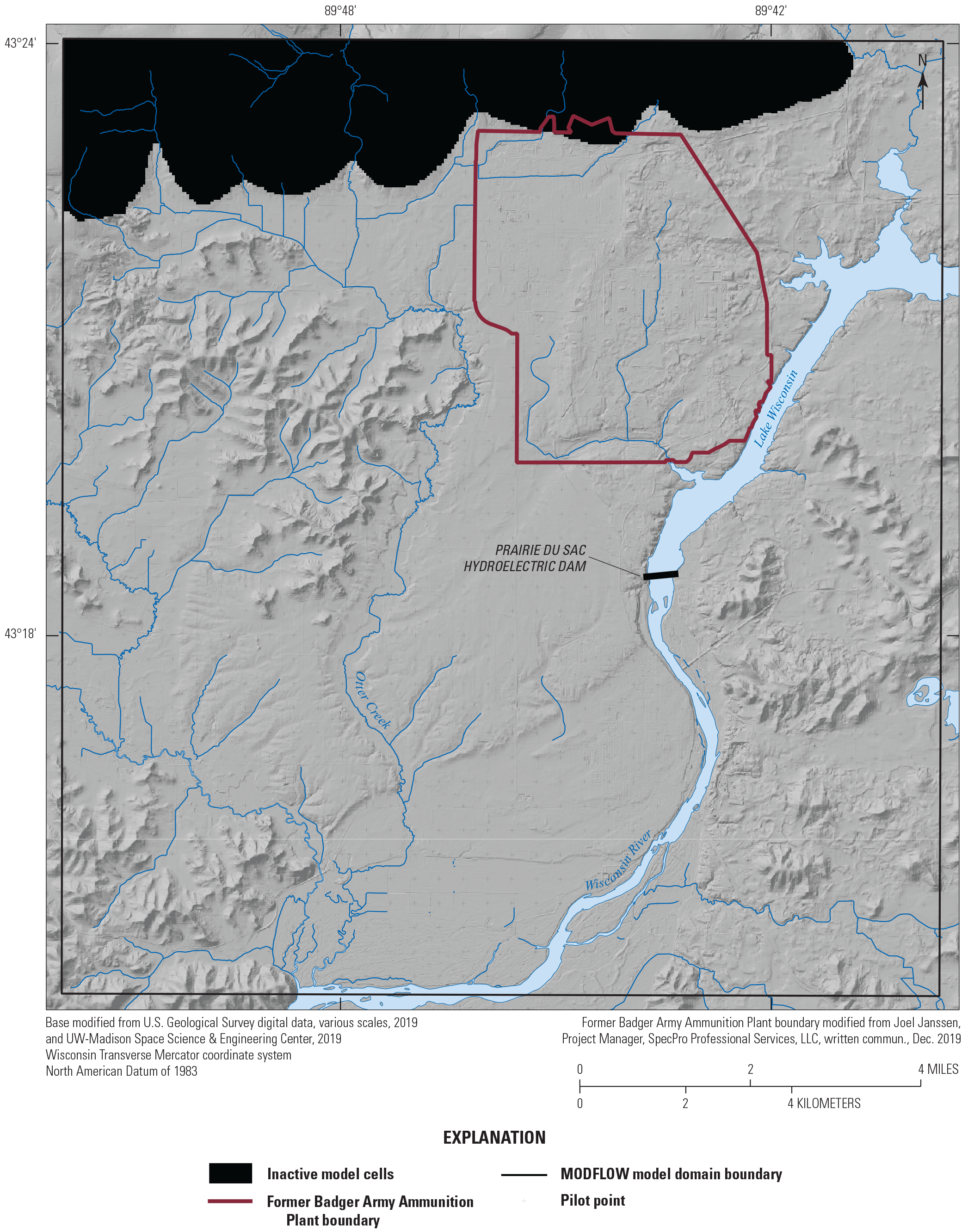
The U.S. Geological Survey (USGS), in cooperation with the U.S. Army Environmental Command (USAEC), built and calibrated a transient groundwater flow model using the Newton Raphson formulation (MODFLOW–NWT) of the U.S. Geological Survey’s modular three-dimensional finite-difference code (Niswonger and others, 2011). The groundwater flow model simulates the groundwater flow system at the former Badger Army Ammunition Plant (BAAP; fig. 1) from 1984 to 2020 to help support remedial efforts at the site. The groundwater flow model was informed by and calibrated to collected field data and focused on the areas where active remediation is being considered for dinitrotoluene (DNT) contamination. Additionally, the model was used to assess the variability of the groundwater system over time and the components of the groundwater budget.
Badger Army Ammunition Plant History
The former BAAP is a 7,275-acre site in Sauk County, Wisconsin (fig. 1). The BAAP was constructed in 1942 and produced smokeless gunpower and solid rocket propellent as munitions components. Peak production periods were during World War II, the Korean War, and the Vietnam War; during these times, the plant employed as many as 7,500 workers. Between peak production periods, the site was maintained with a standby status until a 1997 decision to close the plant permanently (SpecPro Professional Services, LLC, 2019).
During plant operations, waste disposal included burning and burial that, together with wastewater conveyance through open ditches and leaky sewer pipes, have affected the soil and groundwater quality at the former BAAP. Site investigations and restoration began in 1977, and most buildings were removed between 2002 and 2012. Groundwater contamination investigations began in 1980; various remediation actions have occurred since then, and monitoring is ongoing (SpecPro Professional Services, LLC, 2019). Groundwater contamination was discovered in the following plumes (fig. 1):
-
the propellant burning ground (PBG) plume;
-
the deterrent burning ground (DBG) plume;
-
the central plume; and
-
the nitrocellulose (NC) plume.
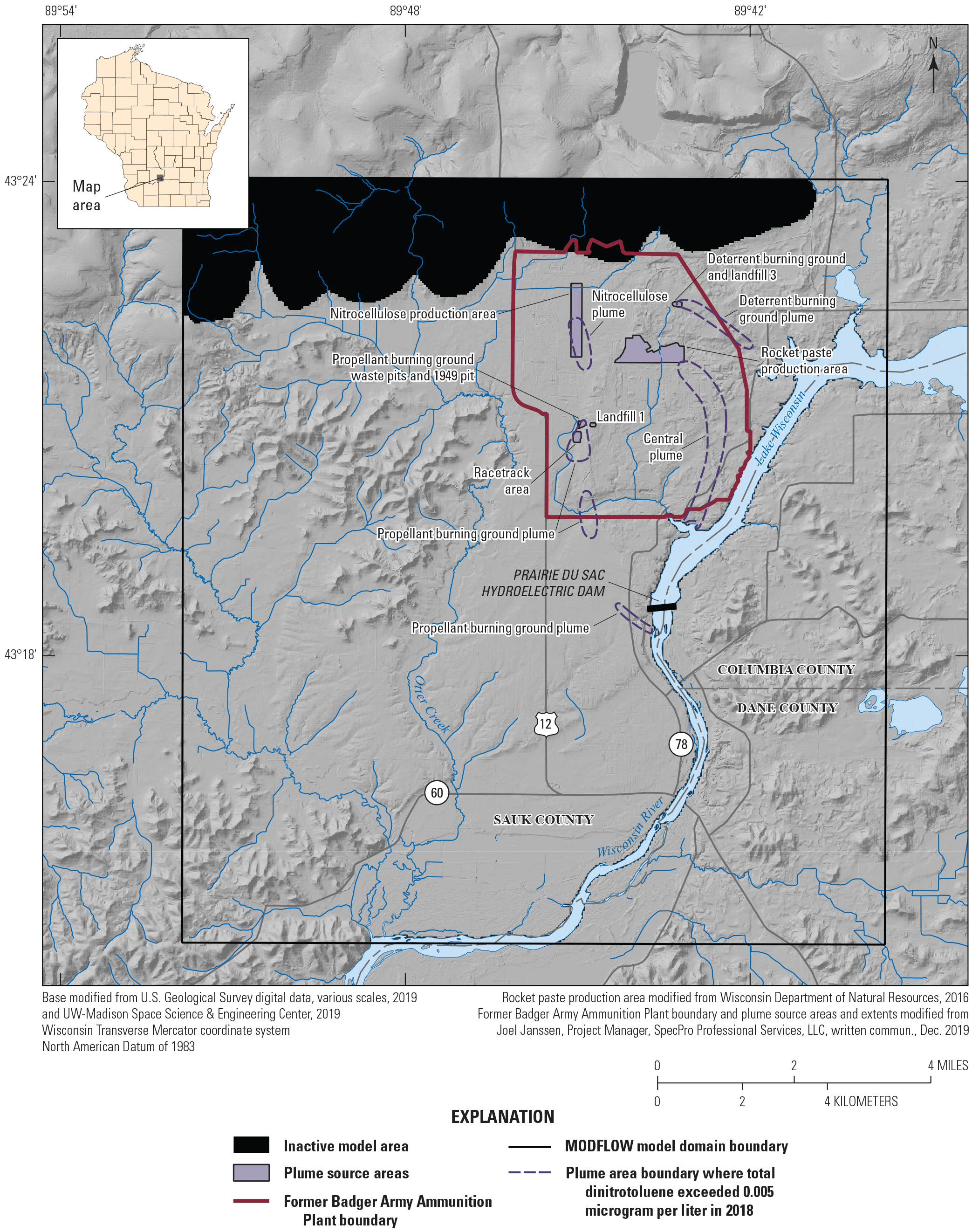
Location of the study site with the former Badger Army Ammunition Plant boundary, major hydrologic features, dinitrotoluene plumes and source areas, and the model domain.
The PBG plume (fig. 1) was first detected in 1982 and has migrated off site from the southwestern corner of the former BAAP site. The contamination source for this plume includes a landfill, several waste pits, and open burning areas (fig. 1; landfill 1, propellant burning ground waste pits, 1949 pit, and the racetrack area). Past remedial activities at the source areas include capping of the waste pits with an impermeable membrane, excavating and disposing contaminated soil, operating a soil vapor extraction system, and operating a bioremediation treatment system. Despite the remedial activities at the source areas, some soil contamination likely remains beneath the caps. In addition to source area remediation, an interim remedial measure (IRM) pump and treat system began operation in 1990 and was expanded with the modified interim remedial measure (MIRM) system in 1996; and additional extraction wells were added in 2005. Together, these systems included varying combinations of source control wells and extraction and boundary control wells. By 2015, the contaminant mass being removed by the pump and treat system had diminished and the system was shut down (SpecPro Professional Services, LLC, 2019).
The DBG plume (fig. 1) has migrated off site from the northeastern corner of the former BAAP site. DBG contamination source areas are a landfill and burn pits where surplus propellant and other site waste were burned during plant operation (fig. 1; deterrent burning ground and landfill 3). Past remedial activities at the DBG source areas include capping of the waste pits with an impermeable membrane, excavating and disposing of some contaminated soil, and operating a bioremediation system. Soil contamination likely remains at the DBG source area beneath the caps and is thought to be more than 20 feet (ft) above the water table (SpecPro Professional Services, LLC, 2019).
The central plume (fig. 1) was discovered in 2004. A defined source area for the central plume is unknown, but the plume is thought to have originated from the north-central part of the former BAAP near the rocket paste production area (fig. 1), which had open ditches that could have leached production wash water through the unsaturated zone to the water table. Past remedial activities include general soil excavation activities near production buildings and along ditches and drainages from the rocket paste and nitrocellulose production areas. Since remediation, it is assumed but not confirmed that the central plume source was eliminated (SpecPro Professional Services, LLC, 2019).
An additional small plume was discovered in 2007 in the northwest corner of the former BAAP. This NC plume (fig. 1) is thought to have originated broadly across the 800-acre smokeless powder and nitrocellulose production areas. Soil testing in this NC production area found DNT contamination likely associated with leaky sewer pipes carrying contaminated wash water and with slab foundation cracks that may have allowed floor wash water to migrate down into the unsaturated zone and then to the water table. Remedial activities have included the removal of the sewer pipes, building slabs, and associated soils in areas with confirmed DNT (SpecPro Professional Services, LLC, 2019).
Contaminants associated with each plume are discussed extensively in SpecPro Professional Services, LLC (2019), a report prepared for the USAEC. The plume contaminants of concern generally include some combination of the six isomers of DNT, total DNT, and various volatile organic carbon compounds. As part of SpecPro Professional Services, LLC (2019), a groundwater human health risk assessment was completed for each contaminant of concern for onsite and offsite groundwater. Based on this risk assessment, the study identified the following human health risk contaminants of concern for each plume:
-
PBG plume: carbon tetrachloride, ethyl ether, trichloroethene, and 2,6-DNT
-
DBG plume: total DNT
-
Central plume: 2,6-DNT
-
NC plume: none
SpecPro Professional Services, LLC (2019) identified potential remedial alternatives for each plume. Based on the remedial alternatives considered, the volatile organic carbon compounds are expected to continue to reduce to acceptable levels through monitored natural attenuation. Active remedial options are being considered by the USAEC for 2,6-DNT in the PBG and central plumes and for total DNT in the DBG plume.
Previous Investigations
Previous groundwater modeling investigations in this area include a GFLOW analytic element groundwater flow model of Sauk County (Gotkowitz and others, 2005), a MODFLOW–NWT model of Columbia County (Gotkowitz and others, 2021), and a MODFLOW model and MT3DMS transport model of the former BAAP site (Zeiler, 2002). The former BAAP site (fig. 1) is at the edges of the Sauk County GFLOW model and the Columbia County MODFLOW–NWT model. Although these county-scale models provide important information about the regional groundwater system, they lack the detail and temporal variability to simulate groundwater flow at the former BAAP at the scale necessary for transport modeling. The Zeiler (2002) MODFLOW and MT3DMS models focused on the transport of carbon tetrachloride during the plant production period through 1998 but did not simulate more-recent groundwater flow conditions or have the large dataset of groundwater elevations collected in the site monitoring wells in the 2000s.
Previous investigations have characterized parts of the groundwater flow system and contamination at the former BAAP. The past remedial activities to reduce the extent and concentration of the groundwater contamination plumes were supported by various studies for the design and implementation of these actions. Notable site studies are summarized in detail in SpecPro Professional Services, LLC (2019). Well construction and groundwater elevation data from site wells are summarized in a Microsoft Access database discussed in appendix 1 (Joel Janssen, Project Manager, SpecPro Professional Services, LLC, written commun., December 19, 2019 [These data are not publicly available. Contact SpecPro Professional Services, LLC, for further information.]). Other previous work, as related to developing the site conceptual model and model layering is discussed in the “Site Description and Hydrologic Setting” section.
Study Overview and Objectives
The USAEC started this study with the USGS to better understand the groundwater flow system at the former BAAP. Specifically, the goals of this study were to (1) create a tool to communicate information about groundwater at the site to local stakeholders, (2) inform the advective component of a future groundwater transport model, and (3) ultimately support future remedial design and implementation at the site. The overall study has two parts. First, create and calibrate a transient groundwater flow model, as summarized in this report. Second, use the flow model to simulate contaminant transport at the site under the USAEC-chosen remedial strategy for each of the plumes. The groundwater flow model was informed by and calibrated to collected field data, including aquifer tests, streamflow measurements, continuous groundwater elevation data, and groundwater gradients with the Wisconsin River. The model simulates the groundwater flow system from 1984 to 2020, a period that begins about when groundwater contamination was discovered on the site and calibration data collection started. The model focuses on the PBG, DBG, and central plumes where active remediation is being considered for DNT contamination. The model was used to assess the variability of the groundwater system over time and the basic components of the groundwater budget.
Purpose and Scope
This report presents the results of an investigation of the groundwater flow system near the former BAAP, including the collection and interpretation of field data and development of a finite difference groundwater flow model. The report includes (1) a description of the hydrologic setting and geology for the groundwater flow model domain (study area); (2) a summary of the field data collection methods; (3) presentation and discussion of field data results; (4) a description of the groundwater modeling approach, including model construction and parameter estimation; (5) a summary of the model results; and (6) a discussion of model limitations and assumptions made during this study. The main body of the text is intended to summarize the study and highlight the key findings. Additional details are provided in the appendixes. All USGS data and models for this study are available in a USGS database. The slug test data (Corson-Dosch and Haserodt, 2023), the Soil-Water-Balance model (Nielsen, 2023), and the MODFLOW–NWT model (Reeves and Corson-Dosch, 2023) are in data releases. Streamflow data and well water level data collected for this study are in the USGS National Water Information System (NWIS; USGS, 2021).
Hydrogeologic Setting and Conceptual Model of the Flow System
The groundwater system at the former BAAP interacts with surface water features including streams, the Wisconsin River, and wetlands across the site. Water enters the groundwater system as rainfall or melted snow, which either routes through surface water features, evaporates, is used by plants, or infiltrates through the land surface to the water table. The water table dips gradually across the former BAAP from the Baraboo Hills towards the Wisconsin River. The depth to the water table exceeds 100 ft in the middle of the former BAAP site, and the unsaturated zone thins to zero towards the Wisconsin River.
Groundwater at the former BAAP site flows through a coarse-grained surficial aquifer developed in a pre-glacial valley of the Wisconsin River and the underlying sedimentary bedrock aquifer. Because of the crystalline Precambrian Baraboo Quartzite, the Baraboo Hills to the north of the site likely form a barrier to groundwater flow and are not part of the aquifer system. Sandstone, dolomite, and shale bedrock units flank the Baraboo Hills and underlie the Wisconsin River valley and the surficial aquifer at the site. These sedimentary bedrock units are part of the regional Cambrian-Ordovician aquifer system. The surficial sediments in the valley range in thickness from thin along the bedrock hills to greater than 300 ft in the middle of the valley, with a saturated thickness of 100 to 225 ft over most of the former BAAP site. The sedimentary bedrock aquifer at the site ranges in thickness from 400 ft under the pre-glacial valley to about 800 ft and overlies Precambrian crystalline basement rocks. Additional detail about the hydrostratigraphy and geology at the site is described in the next two sections.
Water flows from the Baraboo Hills and other topographic highs surrounding the Wisconsin River valley down through the surficial aquifer and towards the Wisconsin River, the primary discharge zone for groundwater in the region. The Wisconsin River flows from northeast to southwest. Upstream from the Prairie du Sac hydroelectric dam (fig. 1) on the Wisconsin River, the river functions more as a lake (locally called “Lake Wisconsin”) near the former BAAP site. The river water level above the dam is artificially raised by nearly 40 ft relative to the downstream river water level. The dam affects the surrounding water table and the vertical hydraulic gradient between the shallow aquifer and river.
Runoff from the Baraboo Hills concentrates into streams that flow across the surficial aquifer, often losing water to the aquifer except where fine-grained sediments are at the surface (generally west of U.S. Route 12; fig. 1) and can impede infiltration. The former BAAP site does not have perennial streams. Otter Creek is the closest perennial stream and flows west of the site (fig. 1) from the Baraboo Hills across the valley and flanks the sedimentary bedrock hills west of the site before discharging to the Wisconsin River. Other surficial hydrologic features include wetlands to the east of the site and in the Wisconsin River bottomlands at the southernmost edge of the study area.
Recharge to the groundwater system is primarily from precipitation that infiltrates from the land surface. Because the surficial sediments across the former BAAP site are generally coarse grained, runoff is likely minimal after precipitation events and snowmelt; and most precipitation would either recharge the groundwater or be lost to evapotranspiration. Additional recharge to the system occurs from runoff from the Baraboo Hills, as described previously, and from any losing sections of streams or rivers.
The Cambrian-Ordovician aquifer units below the surficial aquifer are quite productive at depth and are used for municipal supply and irrigation. The most productive layer in these units is the Mount Simon Sandstone of the Elk Mound Group (hereafter referred to as the Mount Simon Sandstone), which lies below the shaly dolomite unit (Eau Claire Formation of the Elk Mound Group) that forms a leaky hydraulic barrier to vertical flow between the deep bedrock units and the surficial aquifer and shallow bedrock units.
Bedrock and Surficial Geology
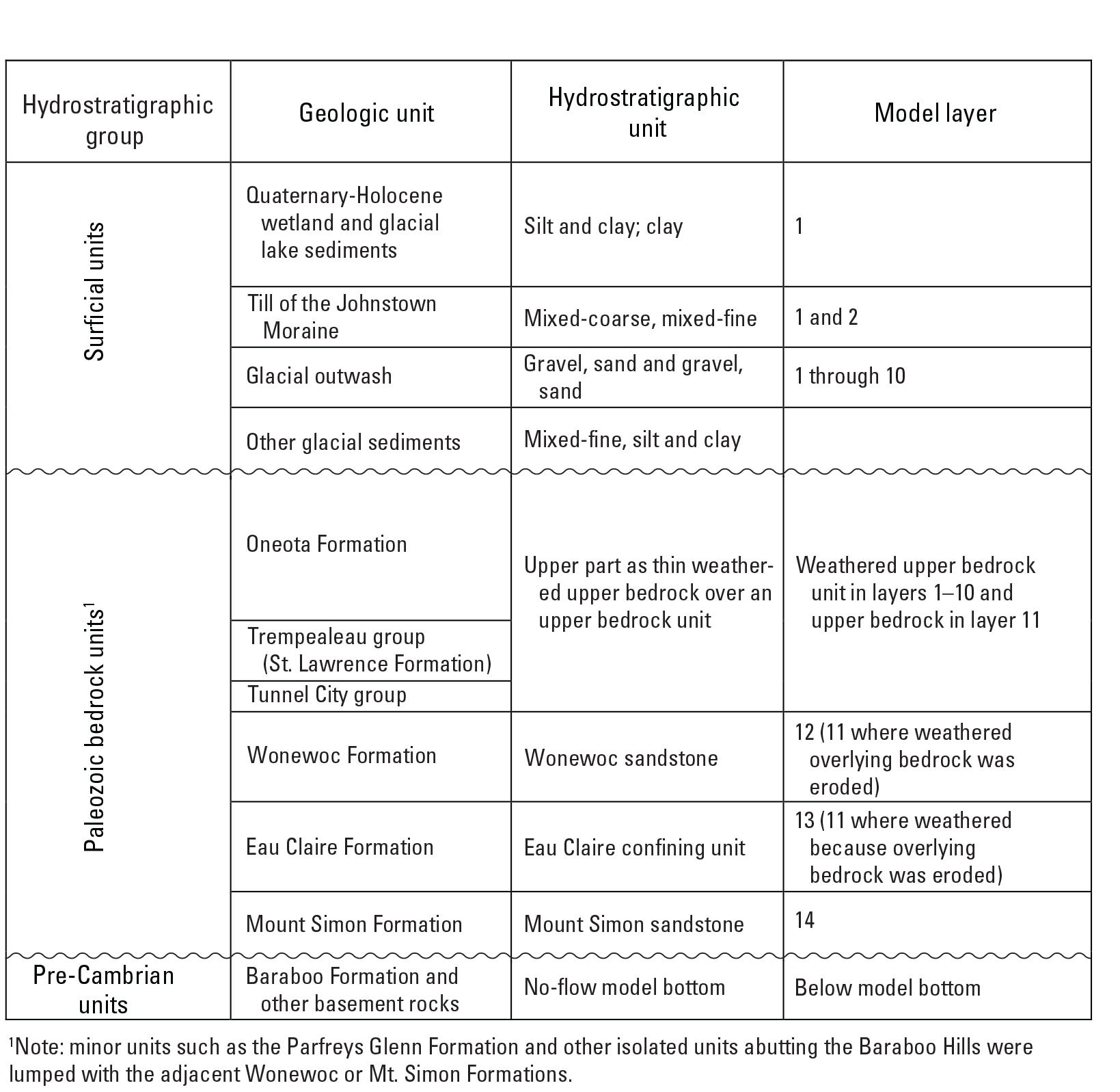
Previous reports on the bedrock and surficial geology of the region informed the geologic model of the former BAAP site and surrounding area (Dalziel and Dott, 1970; Clayton and Attig, 1990; Clayton and Attig, 1997; Brown and others, 2013a,b; Ostrom, 1965; Parsen and others, 2016; Carson and others, 2019; Lundqvist and others, 1993; Krohelski and others, 2000; Gotkowitz and others, 2005). Additional geologic data came from USAEC monitoring well logs (Joel Janssen, Project Manager, SpecPro Professional Services, LLC, written commun., February 1, 2021), Wisconsin Department of Natural Resources county well reports for Dane, Columbia, and Sauk Counties (Wisconsin Department of Natural Resources, 2021), and well logs from Wisconsin Geological and Natural History Survey (WGNHS) online datasets in the area (available through https://wgnhs.wisc.edu/catalog/publication), including the Columbia County groundwater flow model (Gotkowitz and others, 2021), which has the former BAAP site in its northwest corner. The general geology of the site is described in this section of the report, and the conceptualized hydrostratigraphic units for the groundwater flow model are described in the next section. A simplified map of the surficial geology near the site is shown on figure 2. The units in figure 2 are primarily derived from three surficial, glacial, and bedrock geologic maps that cover the study area (Attig and Clayton, 2003; Hooyer and others, 2015; Clayton and Attig, 1997) because no single map covered the surficial units in the study area.
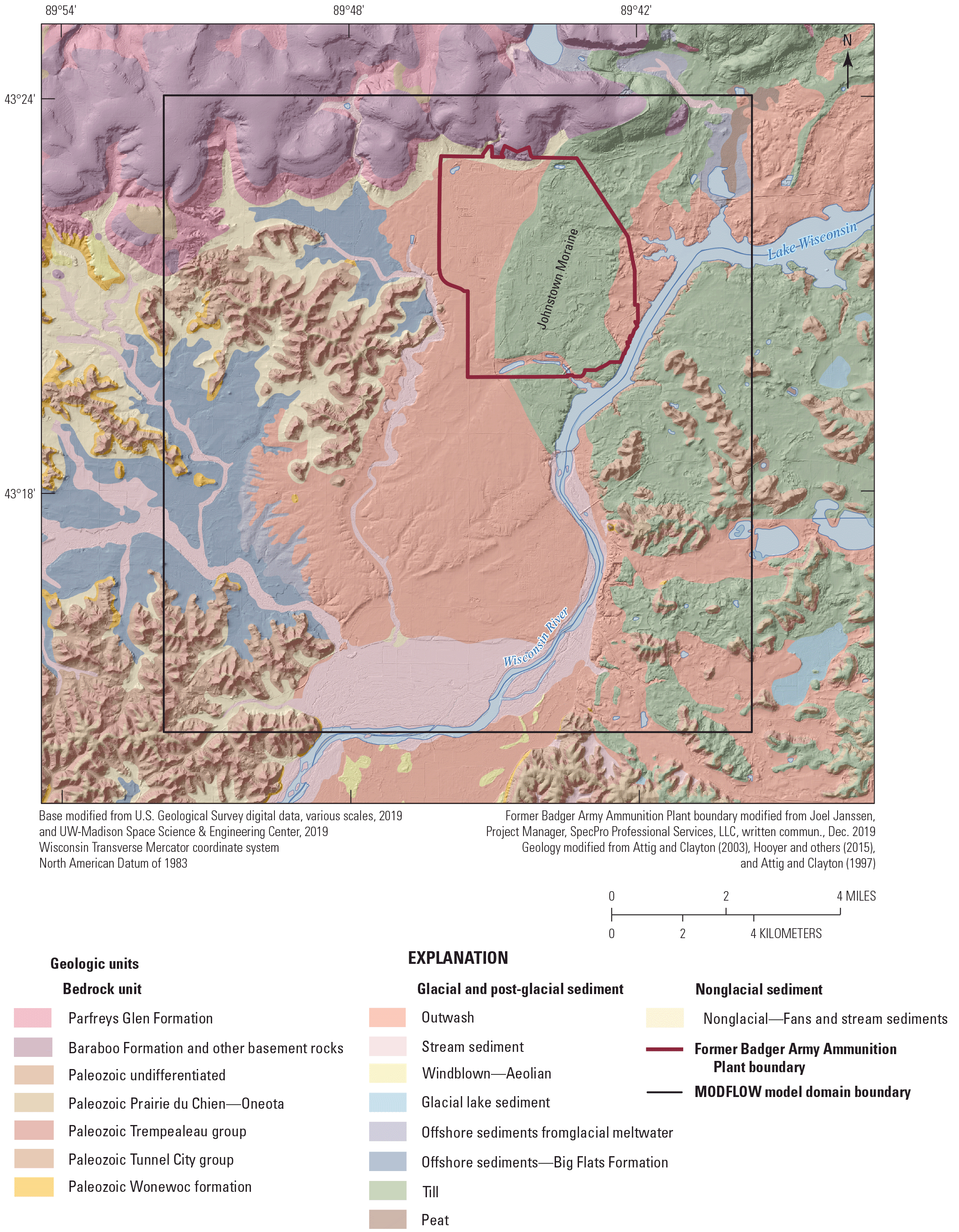
Surficial geologic units for the former Badger Army Ammunition Plant study area.
The former BAAP site sits at the edge of the Driftless Area of Wisconsin (Carson and others, 2019), an area with no evidence of glaciers since the deposition of the Cambrian and Ordovician sediments. The bedrock surface under the former BAAP site and the Wisconsin River valley in this area was cut by an earlier river system that was thought to flow away from the Mississippi River (not shown) rather than towards it as the Wisconsin River does today (Carson and others, 2019). The Johnstown Moraine (Lundqvist and others, 1993; Clayton and Attig, 1990), the farthest western edge of the last glaciation, is in the middle of the former BAAP site (fig. 2). Pro-glacial sediments derived from glacial runoff fill the pre-glacial valley to the west of the terminal moraine (Clayton and Attig, 1990). These sediments and the overlying moraine sediments (Lundqvist and others, 1993; Clayton and Attig, 1990) consist of very coarse- to fine-grained grained outwash sediments, and a sandy till cap that composes the Johnstown Moraine. To the east and north, some of the surficial glacial sediments were deposited in meltwater lakes to the west of the moraine and are more clay-rich (Clayton and Attig, 1990) as shown on the geologic map (Clayton and Attig, 1990, plate 1) and in well logs.
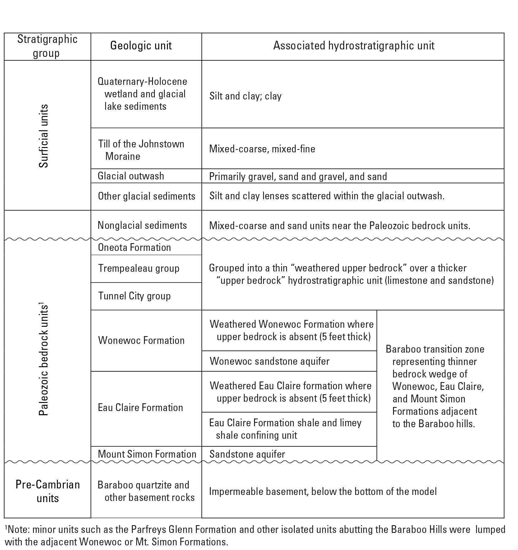
The bedrock geology of the region is composed of the Precambrian Baraboo Quartzite in the Baraboo Hills (figs. 2, 3; Dalziel and Dott, 1970; Clayton and Attig, 1990), an erosional remnant of the Canadian Shield rocks that underlie all of Wisconsin. These older rocks are flanked by Cambrian- and Ordovician-aged sedimentary rocks deposited in a shallow sea above the Precambrian surface (Dalziel and Dott, 1970; Clayton and Attig, 1990). These younger strata, as described in Dalziel and Dott (1970) and Clayton and Attig (1990) unless otherwise noted are, from oldest to youngest; the Parfreys Glen Formation (Clayton and Attig, 1990), a quartzite conglomerate and sandstone that laps against the Baraboo Quartzite; the Mount Simon Formation (fig. 3), a sandstone that does not crop out in the area (based on drill cuttings, the unit underlies the shallower bedrock units and is known to be greater than 200 ft thick); the Eau Claire Formation of the Elk Mound Group (hereafter referred to as the Eau Claire Formation), a heterogeneous unit composed of siltstone, shale, dolostone, and fine sandstone that also does not crop out in the study area but is interpreted from drilling; the Wonewoc Formation of the Elk Mound Group (hereafter referred to as the Wonewoc Formation) (figs. 2, 3; Ostrom, 1965), the oldest of the sedimentary units that crops out at land surface in the study area, that is a well sorted sandstone exposed under the bottom of the pre-glacial river valley; the Tunnel City Group, a dolomitic fine sandstone with thin dolomite layers about 100 to 150 ft thick; and the rocks of the Trempealeau Group, which most commonly are exposed on the hills on the east and west side of the Wisconsin River valley. The Trempealeau Group includes dolomite and siltstone of the St. Lawrence Formation and the Jordan Formation sandstone above. The topmost stratigraphic unit of the study area is the Oneota Formation, a dolomite that forms the caprock of many of the hills. Bedrock units that crop out in the study area are shown on the surficial geology map (fig. 2). The glacial and bedrock sequence is shown in a stratigraphic chart in figure 3.
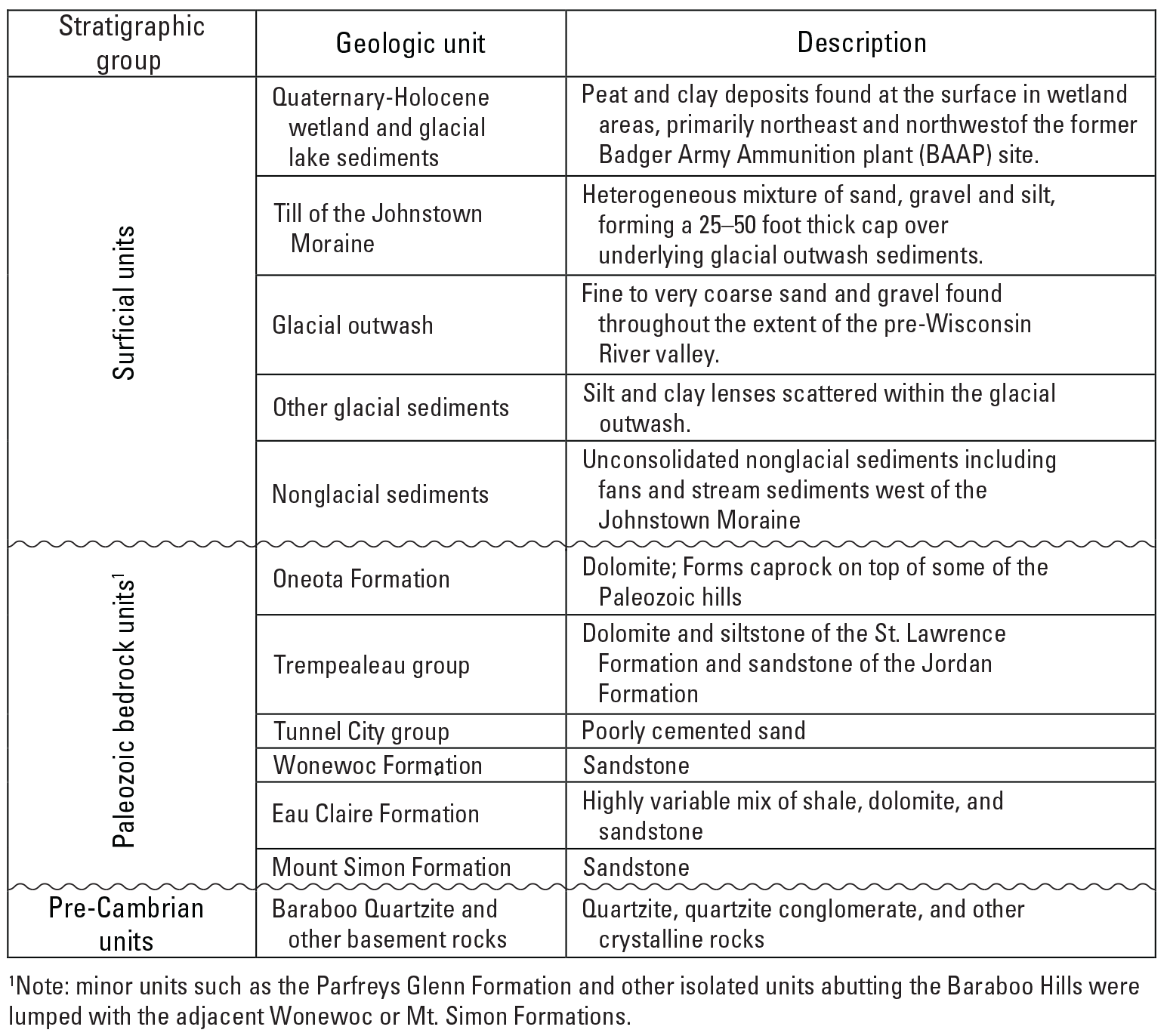
Geologic units in the former Badger Army Ammunition Plant study area.
Many of the bedrock units also have a weathered saprolite layer where they have been exposed to the surface and chemical erosion, especially to the west of the terminal moraine. The saprolite zones are not listed specifically in figure 3 but were added to the group of hydrostratigraphic units represented in the model.
Hydrostratigraphic Units
For the former BAAP groundwater model, the unconsolidated and geologic units at the site and the surrounding area were divided up into hydrostratigraphic units based on the lithology, depositional history, and water-bearing characteristics of the units. The bedrock units were generally assigned to hydrostratigraphic units based on the specific formations, but the surficial units were broken down into texture-based hydrofacies representing different sediment sizes.
Texture-based hydrofacies were used to classify the surficial hydrostratigraphic units for two reasons: (1) because well logs, the primary source of information used in the classification, describe the sediments using textural descriptions, and (2) this type of classification provided convenient categories to facilitate the model calibration of hydraulic conductivity for the upper unconsolidated model layers. Seven texture-based hydrofacies were used in the surficial hydrostratigraphic unit classification: gravel, sand and gravel, sand, mixed-coarse, mixed-fine, silt and clay, and clay. The mixed-coarse and mixed-fine facies were used when an interval in the log contained a mix of coarse-grained and fine-grained sediments but either the coarse fraction or fine fraction was dominant. The other facies were used when the log interval description was relatively uniform. Additional detail about the hydrofacies model development is presented in appendix 3.
The hydrofacies across the model domain are dominated by coarse-grained sediments, such as gravel, mixed sand and gravel, and sand, which is a good representation of the outwash sand and gravel deposits that dominate the study area (fig. 2). Because the water table across much of the former BAAP site is 25–50 ft below the bottom of the surficial sandy till of the Johnstown Moraine, the uppermost hydraulically active hydrofacies are the coarser-grained outwash deposits that are found under the surficial till. Fine-grained silt and clay deposits are most common to the north of Lake Wisconsin as well as northwest and east of the former BAAP site. A series of three-dimensional views of the hydrofacies model (fig. 4) illustrates the distribution of the units across the study area. The method used to classify the surficial geology for the groundwater flow model is described in appendix 3.
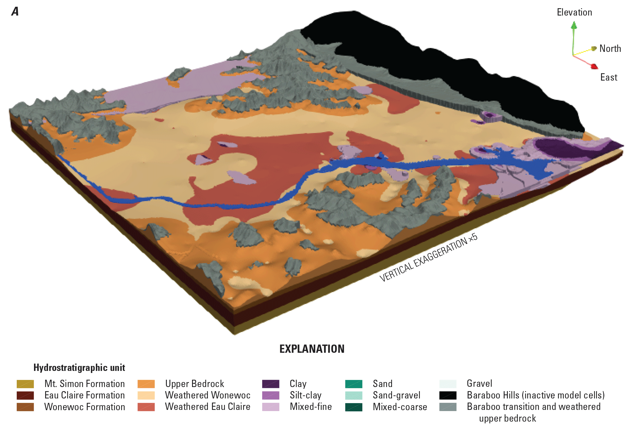
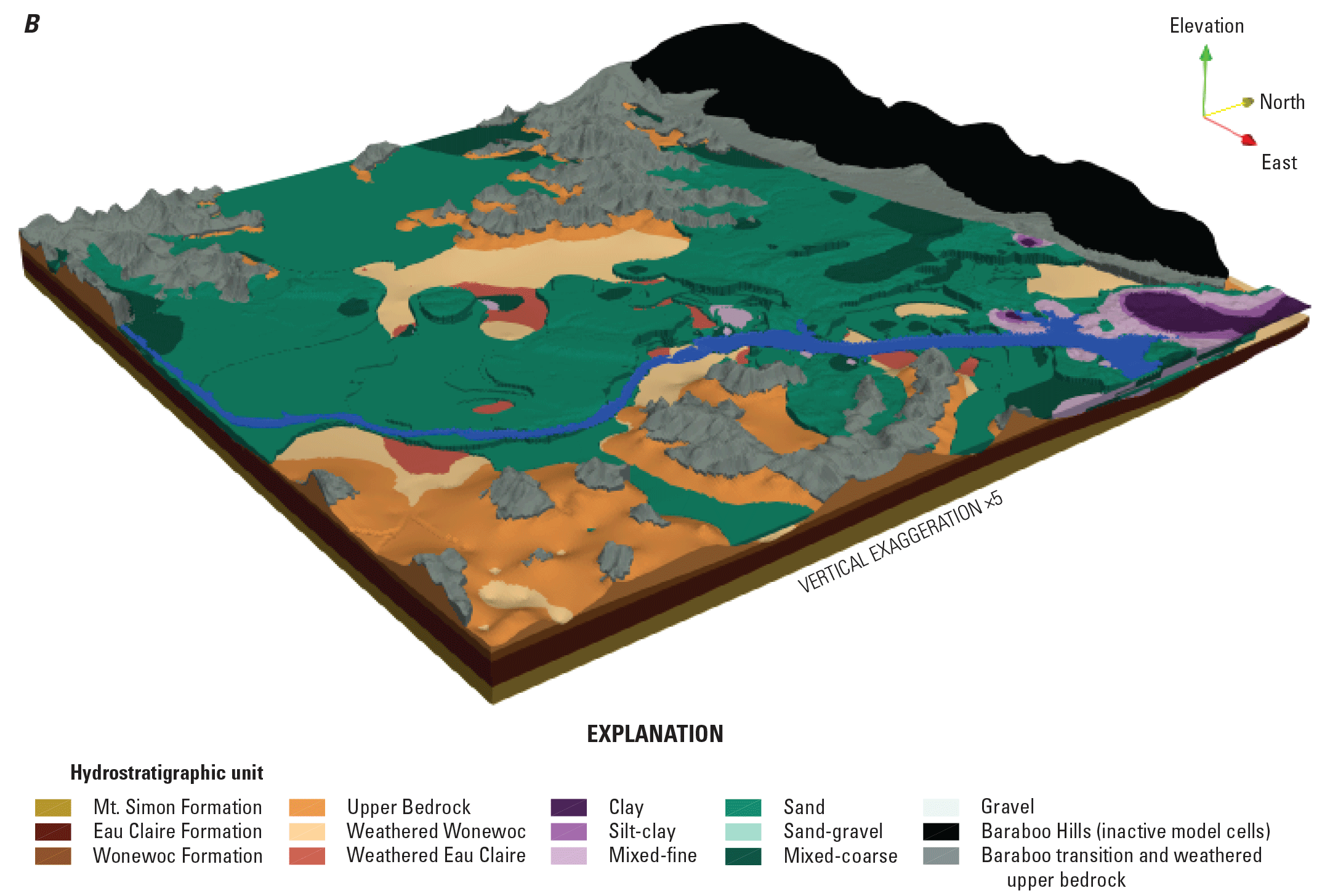
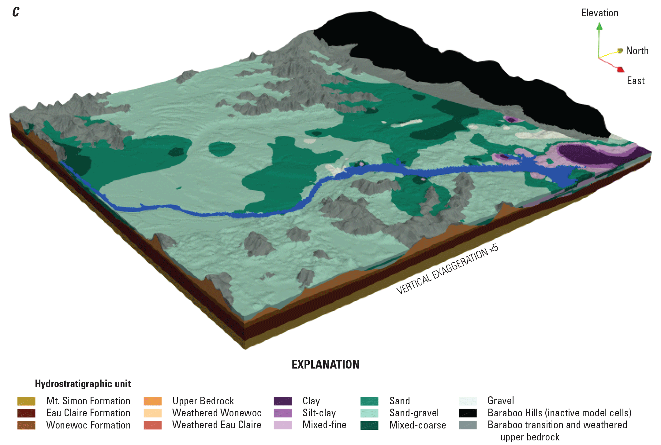
Surficial hydrofacies model for the former Badger Army Ammunition Plant study area moving from deeper to shallower sediments. Areas where sediments are absent show the upper bedrock unit. From deep to shallow are, A, fine grained sediments; B, fine grained and medium grained sediments; and, C, coarse grained sediments.
The hydrostratigraphic units (fig. 5) in the bedrock were simpler to assign because they correspond to the geologic formations. Because of their position in the landscape (forming the hills on either side of the Wisconsin River valley) and the depth to groundwater within them, the Tunnel City Group, Trempealeau Group, and Oneota Formation are lumped together as one unit for the purposes of the groundwater flow model. These form the uppermost bedrock hydrostratigraphic unit called the “upper bedrock” unit. Below the Tunnel City Group, the Wonewoc Formation is the next hydrostratigraphic unit and is present under much of the surficial sediments in the bedrock valley, although it is a relatively thin unit; and the bedrock surface is scoured below the bottom of the Wonewoc in the deepest parts of the bedrock valley below the Wisconsin River. Below the Wonewoc, the Eau Claire Formation is a thick unit above the lowest unit, the sandstone Mount Simon Formation. The Eau Claire Formation contains layers of shale, siltstone, and dolomite that form an effective confining layer between the upper sandstone of the Wonewoc and the lower Mount Simon Formation.
Hydrostratigraphic units used in the study area for the groundwater flow model layering.
Field Data Collection Methods, Analysis, and Results
This section summarizes the field data that were collected for this study between November 2020 and December 2021, and briefly describes methods and key results. Field data are available in the National Water Information System (NWIS; USGS, 2021) and the companion data release (Corson-Dosch and Haserodt, 2023) and include the following:
-
hydraulic heads in the riverbed relative to the corresponding water elevation in the Wisconsin River,
-
continuous groundwater elevations from nested well pairs in the DBG and PBG plume source areas,
-
slug tests in well across the site to estimate horizontal hydraulic conductivity, and
-
quarterly, synoptic streamflow measurements along Otter Creek.
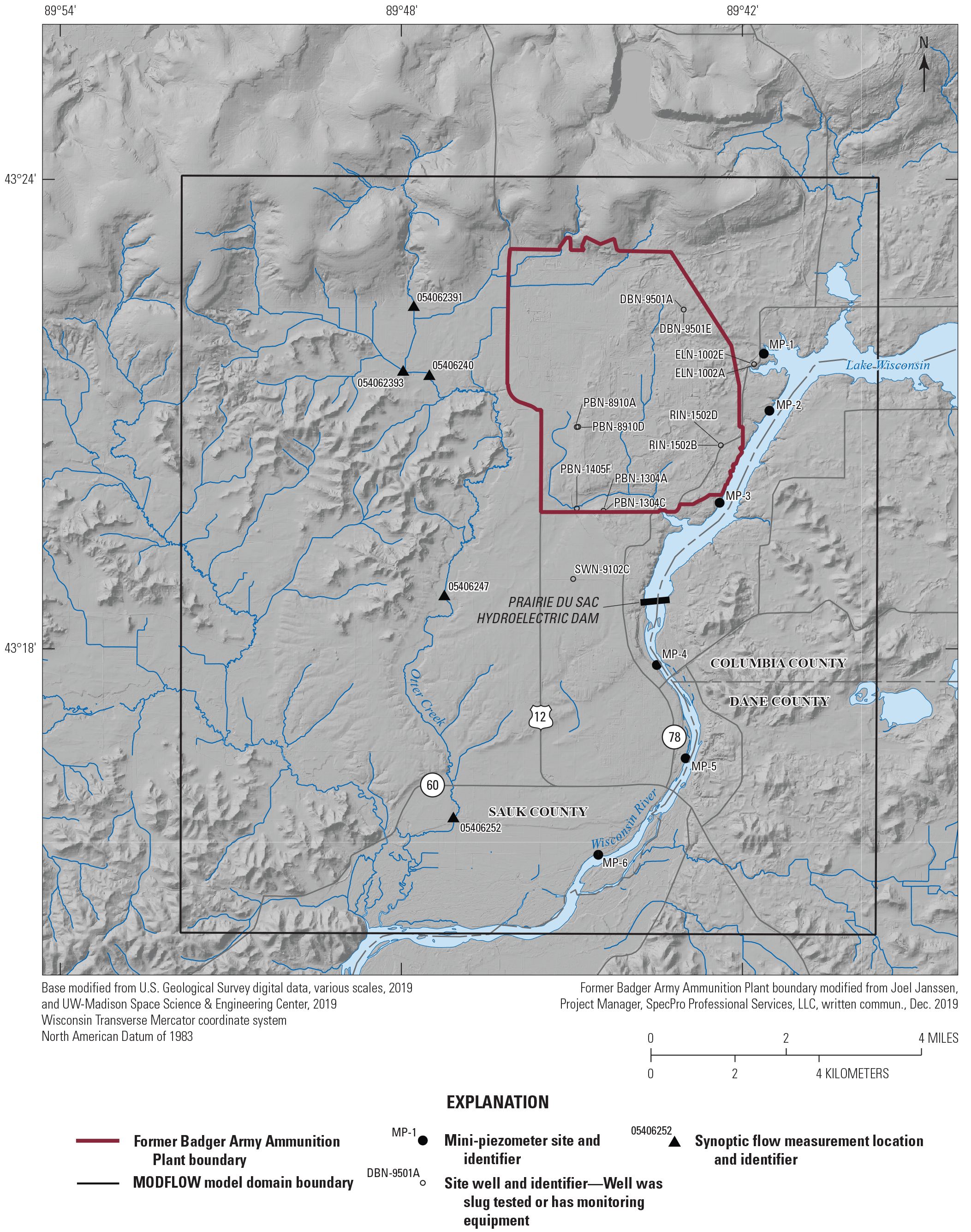
Field data collection locations for the mini-piezometers, synoptic flow measurements, and site wells used for either slug testing or continuous water level measurements.
Mini-Piezometers
Six mini-piezometers were installed along the Wisconsin River (fig. 6) to assess the vertical hydraulic gradient between the shallow groundwater system and the Wisconsin River within the study area. The mini-piezometer locations were selected to assess spatial variability in the vertical hydraulic gradients upstream and downstream from the Prairie du Sac hydroelectric dam.
Field Methods and Data Analysis
Mini-piezometers were constructed from 0.5-inch high-density polyethylene tubing and a short screen made of tubing with drilled holes wrapped in porous cloth to allow water to enter but prevent sediment from clogging the screen. The mini-piezometers were installed into the sandy riverbed along the banks at depths of 2.5–6.8 ft below the riverbed and allowed to equilibrate for at least 24 hours. An overview of the mini-piezometer construction details is provided in table 1, and additional information is available in NWIS (USGS, 2021).
The depth to groundwater was measured from an established measuring point on the mini-piezometers using a steel water level tape following methods by Cunningham and Schalk (2011). A simultaneous depth to the river surface was also collected from the measuring point. A top of casing elevation and location was established for each mini-piezometer using a survey-grade Global Positioning System.
A vertical hydraulic head difference between the river and the shallow groundwater system was calculated as the groundwater elevation in the mini-piezometer minus the river elevation at the mini-piezometer location; positive values indicate groundwater is discharging to the Wisconsin River, and negative values indicate river water is flowing downward into the aquifer.
Table 1.
Mini-piezometer well construction details, groundwater and river elevations, and calculated vertical hydraulic head differences.[Data are summarized from the National Water Information System (NWIS) database (U.S. Geological Survey, 2021). Positive hydraulic head differences indicate groundwater is discharging to the Wisconsin River, and negative values indicate river water is flowing downward into the aquifer. ID, identifier; NAVD 88, North American Vertical Datum of 1988]
| Site ID (fig. 6) | NWIS mini-piezometer site number | NWIS river elevation site number | Total well depth, in feet | Well screen length, in feet | Groundwater elevation on November 6, 2020, in feet above NAVD 88 | River elevation on November 6, 2020, in feet above NAVD 88 | Hydraulic head difference between the river and shallow groundwater, in feet |
|---|---|---|---|---|---|---|---|
| MP–1 | 432146089413701 | 432146089413702 | 2.83 | 0.7 | 774.27 | 774.25 | 0.02 |
| MP–2 | 432102089413101 | 432102089413102 | 2.46 | 1 | 774.34 | 774.24 | 0.10 |
| MP–3 | 431952089422401 | 431952089422402 | 6.81 | 1 | 771.58 | 774.22 | −2.64 |
| MP–4 | 431748089433001 | 431748089433002 | 2.46 | 1.1 | 731.33 | 731.09 | 0.24 |
| MP–5 | 431636089430001 | 431636089430002 | 3.31 | 0.85 | 730.61 | 730.57 | 0.04 |
| MP–6 | 431522089443201 | 431522089443202 | 2.8 | 0.7 | 728.48 | 728.34 | 0.14 |
Results and Discussion
The mini-piezometers (fig. 6) showed groundwater discharging (table 1) to the Wisconsin River at all locations, except MP–3, which is 1.8 miles upstream from the dam. This is consistent with the conceptual model that the river is a strong regional groundwater sink, except for just upstream from the dam where the river stage is artificially elevated above the water table and the river becomes a water source to the groundwater system. This zone of gradient reversal likely extends at least 1.8 miles upstream from the dam to MP–3 and switches back by MP–2 (3.3 miles upstream from the dam). This is consistent with the dam backwater effect lessening with distance upstream. The largest positive hydraulic head difference was just below the dam where a rapid hydraulic head drop across the dam likely drives concentrated groundwater discharge.
Continuous Groundwater Elevations
Field Methods
Groundwater levels were measured hourly in 2 well nests consisting of a paired shallow and deep well near the PBG (PBN–8910A, NWIS site 432050089445301; and PBN–8910D, NWIS site 432050089445501) and DBG (DBN–9501A, NWIS site 432221089430201; and DBN–9501E, NWIS site 432220089430201) sources areas (fig. 6). Groundwater levels were measured using pressure transducers following standard USGS procedures (Cunningham and Schalk, 2011).
Otter Creek Synoptic Streamflow Measurements
Field Methods
Starting in the summer of 2020, quarterly synoptic streamflow surveys were done at five sites (fig. 6) along Otter Creek. Data presented in this report were collected through the fall of 2022. The streamflow survey targeted baseflow conditions where the streamflow is predominantly derived from groundwater. The streamflow measurements were collected using standard USGS methods in Turnipseed and Sauer (2010). The purpose of the synoptic streamflow measurements was to identify areas of the creek that were gaining or losing water to/from the groundwater system. This information informed the model calibration.
Results
Data from the synoptic streamflow survey are available in NWIS (USGS, 2021) using the site numbers (figs. 6, 7). Some sites had fewer measurements because of unfavorable measuring conditions. The highest streamflow values were from the spring 2021 and 2022 baseflow measurements. Streamflow generally increased in the headwaters of Otter Creek until the stream section between sites 05406240 and 05406247, where streamflow was relatively flat or slightly losing. Flows then decreased between sites 05406247 and 05406252, which indicates that Otter Creek is losing water to the groundwater system somewhere along this stretch. Overall, Otter Creek seems to gain water in the upper part of the watershed and then lose flow in at least parts of the middle to lower watershed.
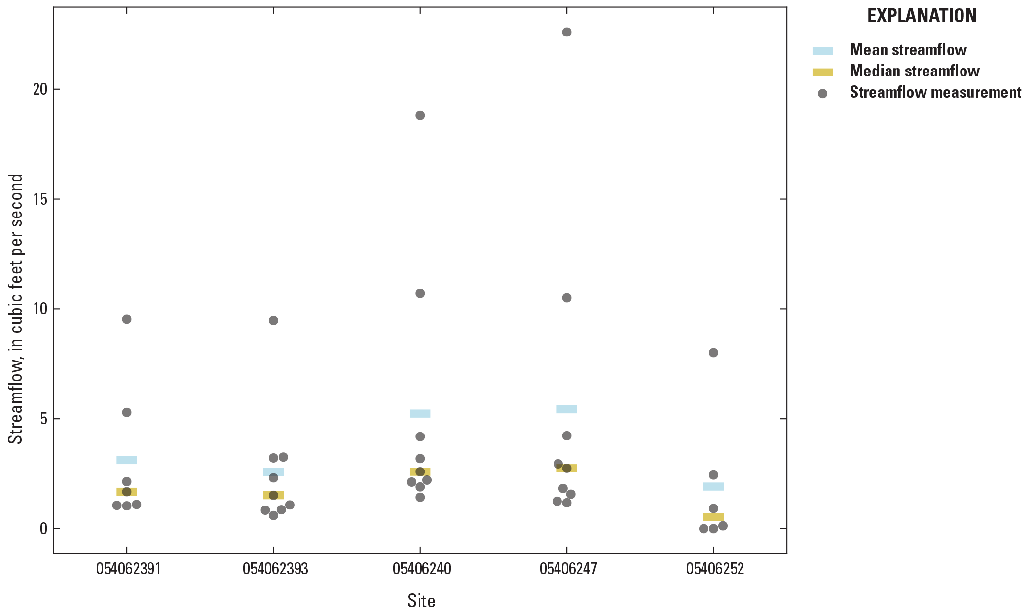
Streamflow results from the synoptic streamflow survey.
Slug Tests
Field Methods
Rising-head and falling-head slug tests were performed at 12 wells on November 18–19, 2020 (fig. 6) to estimate horizontal hydraulic conductivity (Kh) in the unconsolidated and bedrock aquifers. Generally, one rising-head test and one falling-head test were completed at each well, except for well RIN–1502D, where only one rising-head test result was used. These tests supplemented existing Kh estimates from earlier tests (ABB Environmental Services, Inc., 1993) with the objectives of (1) improving the spatial coverage of Kh estimates across the former BAAP, with particular emphasis on adding Kh estimates in areas downgradient from contamination that have sparse data; and (2) estimating Kh in shallow-deep well pairs to evaluate vertical Kh heterogeneity in unconsolidated aquifer materials.
For each rising- or falling-head slug test a solid polyvinyl chloride slug was rapidly added (falling-head test) or removed (rising-head test) from the well. Water-level measurements were recorded with a submersible pressure transducer. Manual depth-to-water measurements were also collected simultaneously using an electronic water level meter to verify transducer readings. Because of the short duration of all tests (generally less than 10 minutes and all tests less than 65 minutes), changes in barometric pressure during the tests were assumed to be negligible.
Slug Test Analysis
Slug test water level data were analyzed with the AQTESOLV program (version 4.5; Duffield, 2007) using the solution method judged to be most appropriate based on well construction (all wells were partially penetrating) and the water level response to the slug (oscillatory or nonoscillatory). The solution methods used included the Kansas Geological Survey method for unconfined or confined settings (Hyder and others, 1994), and the Springer-Gelhar method (Springer and Gelhar, 1991) for unconfined. The Kansas Geological Survey method was used to analyze nonoscillatory data, and the Springer-Gelhar method was used to analyze oscillatory data. Nonoscillatory responses are common during slug tests in wells screened in aquifers with relatively low or medium hydraulic conductivity, whereas oscillatory responses may be observed during slug tests in wells screened in aquifers with high hydraulic conductivity (Duffield, 2007). Well construction information from well construction logs (Joel Janssen, Project Manager, SpecPro Professional Services, LLC, written commun., December 19, 2019) was used by AQTESOLV for both methods of analysis. Example AQTESOLV results from well PBN–1304C are shown in figure 8. The plot shows normalized head (observed water-level displacement divided by the initial displacement) with respect to elapsed time since the start of the slug test and the Kansas Geological Survey model fit to those data.
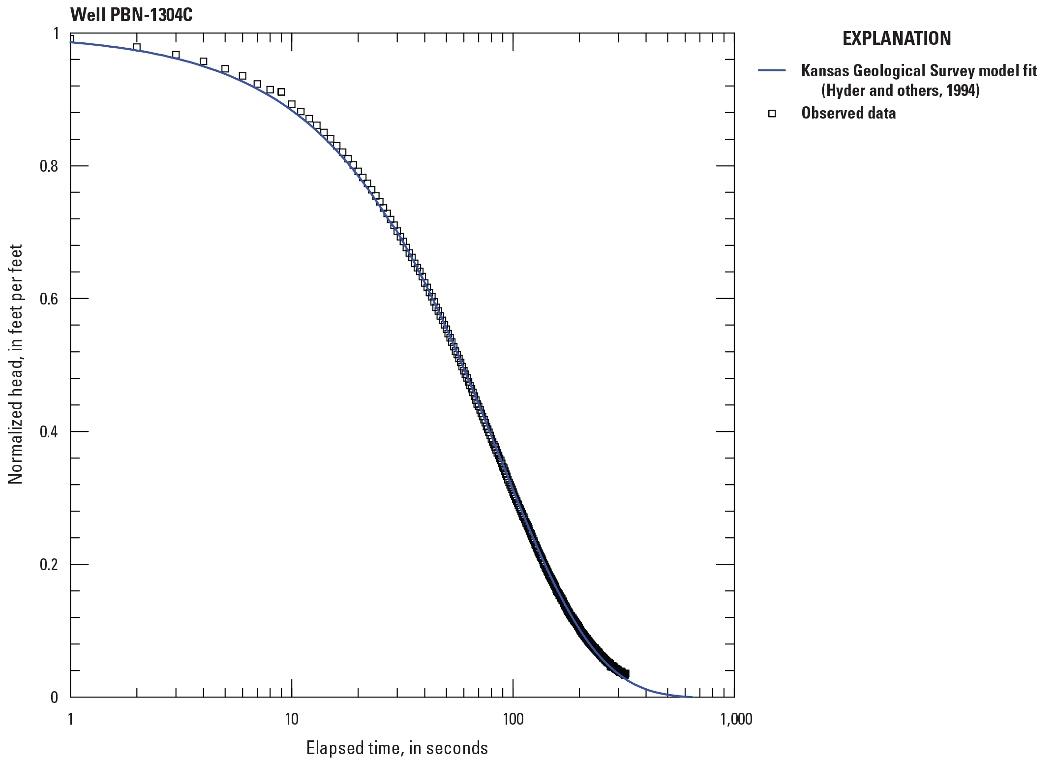
Example graphical slug test analysis output from AQTESOLV for well PBN–1304C.
Slug Test Results
The results of the AQTESOLV slug test analyses are summarized in table 2. Estimated values of Kh are in good agreement with the expected ranges for the lithologies reported (Joel Janssen, Project Manager, SpecPro Professional Services, LLC, written commun., December 19, 2019) at the well screen (Bouwer, 1978). Accordingly, slug test results indicate higher Kh values from wells screened in coarse, unconsolidated sediments and lower Kh values in bedrock and fine-grained sediments. The range of Kh estimates from this study also compares favorably to earlier estimates from slug test data at the former BAAP (ABB Environmental Services, Inc., 1993). Generally, differences in estimates from rising- and falling-head tests were small relative to estimated Kh. However, at certain wells, estimates produced using rising- and falling-head test data were notably different (the largest difference was at well PBN–8910A, where the estimated Kh was 3,561 feet per day (ft/d) for the falling-head test and 318 ft/d for the rising-head test). These differences can likely be attributed to inconsistencies in field methods. Although all Kh estimates produced from rising- and falling-head tests reported in this study seem reasonable based on the lithology reported at the well screen, additional, repeated tests would likely reduce the uncertainty of these estimates. For this reason, it is expected that the average Kh values reported in table 2 provide the most representative estimate of Kh at the former BAAP. Furthermore, it is recommended that the absolute difference in Kh, reported in table 2, be used as a measure of Kh estimate uncertainty. The data release (Corson-Dosch and Haserodt, 2023) contains slug test water-level data, AQTESOLV files, and results for all tests performed as a part of this study.
Table 2.
Summary of horizontal hydraulic conductivity values from slug tests, estimation methods used, and subsurface lithology at the well screen as reported on boring logs.[Data are summarized from Corson-Dosch and Haserodt (2023). Dates are given in month/day/year. Kh, horizontal hydraulic conductivity; KGS, Kansas Geological Survey (method by Hyder and others, 1994); --, no data; Springer-Gelhar, method from Springer and Gelhar (1991)]
Groundwater Flow Model Construction
A numerical model of groundwater flow (Badger model) was developed to simulate the groundwater flow system in the model domain (fig. 1) using MODFLOW–NWT (Niswonger and others, 2011). The Badger model focuses on the transient fluxes through the glacial and bedrock hydrostratigrahic units from October 1, 1984, through September 30, 2020. A particle-tracking model was used to compare the simulated paths of contaminant movement (via advection) in the groundwater with observed plume footprints. Particle tracking was done with MODPATH Version 7 (Pollock, 2016). All model input and output files are provided in the accompanying model data (Reeves and Corson-Dosch, 2023).
Discretization
The Badger model has a regular grid with a uniform horizontal cell size of 150 ft by 150 ft. The model area is subdivided into 392 rows and 362 columns with 14 numerical layers. Model cells covering the Baraboo Hills were set to inactive because of limited groundwater flow potential through the Precambrian bedrock. Of the total 1,986,656 model cells, 214,788 are inactive. MODFLOW convertible layers are used so that the model calculates the altitude of the water table while accounting for unconfined conditions.
Model layers 1–10 represent the unconsolidated materials above the bedrock, and layers 11–14 represent the bedrock units. Table 3 provides a summary of the geologic units represented by each model layer. Figure 9 has a map of bedrock surface and cross sections of the model layers across the model domain. Layer elevations were assigned using the following logic:
-
The model top elevation was assigned using the land-surface elevation from light detection and ranging data (USGS, 2019; University of Wisconsin–Madison, 2019a,b36).
-
The bottom elevation of layer 1 was set at 10 ft below the estimated water table depth from the Columbia County model (Gotkowitz and others, 2021) to minimize the occurrence of dry model cells while allowing for multiple numerical layers to simulate potential vertical movement of groundwater near the contaminant plumes. Layer 1 thickness ranged from 1.1 to 193.7 ft; mean thickness was 48.9 ft. Layers 1 and 2 were thinner to allow for more precision in representing the shallow flow field.
-
The unconsolidated layers 2–10 were assigned thicknesses from the top down until the total unconsolidated thickness was reached. Each layer has a maximum thickness (layer 2: 10 ft, layer 3–6: 25 ft, layers 7–10: 50 ft). If there was less unconsolidated material to assign than the maximum thickness allowed, the actual remaining thickness was assigned. Layers were assigned a pinched-out thickness of 0.1 ft in areas where the unconsolidated was absent or with total unconsolidated thickness was already represented in overlying layers. Layer 10 was entirely pinched out.
-
The top of layer 11 represents the top of the bedrock surface (fig. 9), which is described in appendix 3. For areas near the plumes where the upper bedrock hydrostratigraphic units have been eroded (see cross sections in fig. 9), layer 11 is a 5-ft thick layer of whatever the uppermost bedrock unit is (either weathered Eau Claire Formation when the Wonewoc Formation is eroded or weathered Wonewoc bedrock when present). This thin weathered zone was separated to represent saprolitic zones near the top surface of the bedrock where weathering can increase permeability. This thin “receptor” layer was also added in preparation for future transport modeling. Having a thin layer representing the top of the bedrock allows for future estimation of contaminant concentrations in parts of the plume that may have reached the top of the bedrock. Alternatively, a thick upper bedrock layer could result in undersimulation of contaminant concentration in the upper bedrock by distributing that mass across a larger volume. This receptor layer also approximately corresponds to the screened interval of many wells open to the top of the bedrock. In areas distant from the plumes, where the upper bedrock hydrostratigraphic unit is generally present, layer 11 represents the full thickness of that combined bedrock unit, which includes the Trempealeau Group, the Tunnel City Group, and the Oneota Formation. The hydrostratigraphic units represented by layer 11 are shown in figure 10.
-
Layers 12–14 represent lower bedrock units including the unweathered Wonewoc, unweathered Eau Claire, and Mount Simon Formations, as described in figure 10. The process to determine these bedrock surfaces is described in appendix 3.
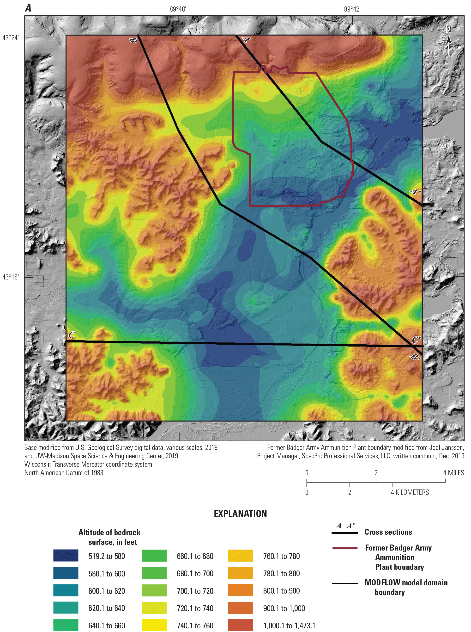
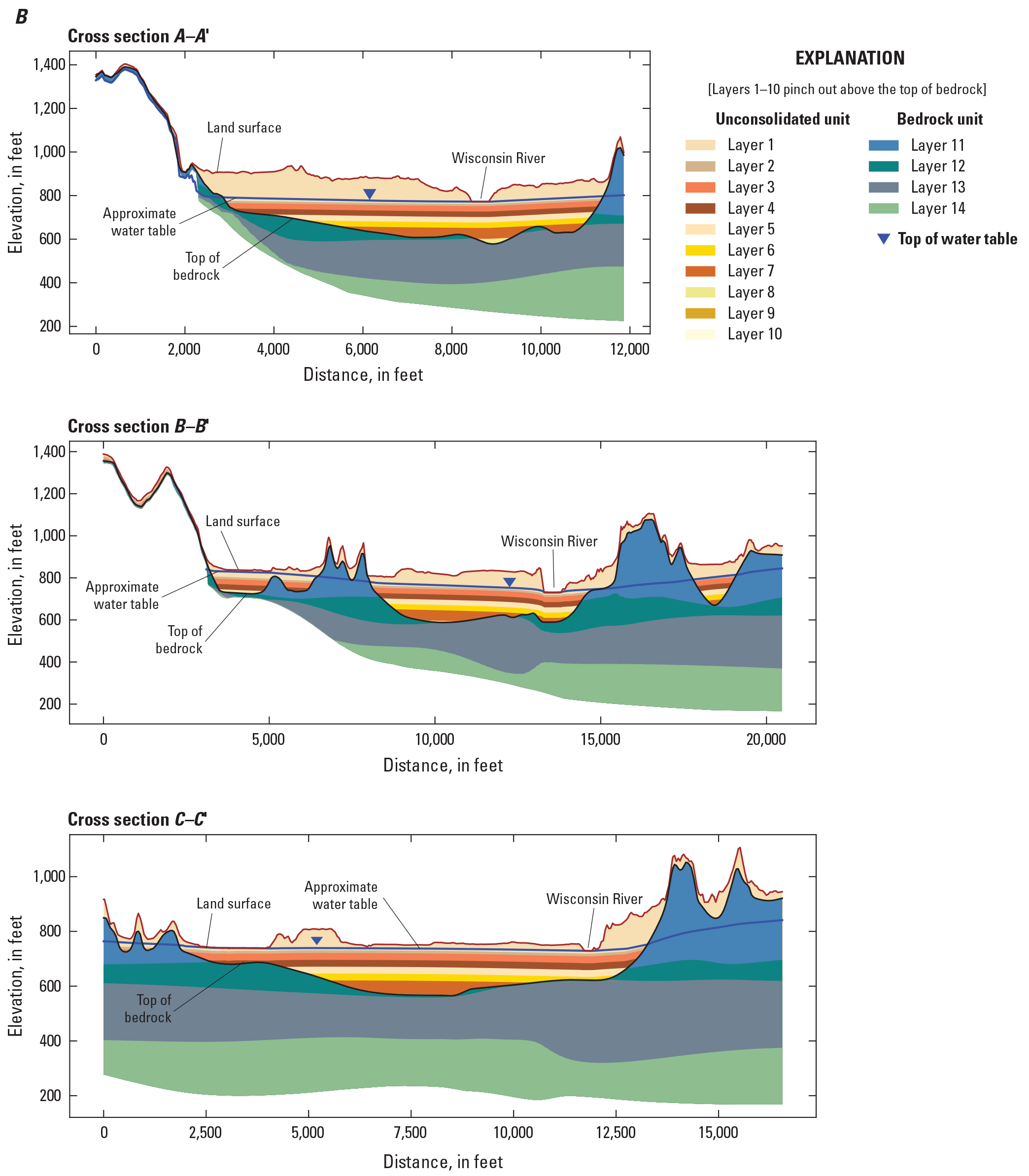
A, altitude of bedrock surface for the study area; and, B, model layers for cross sections A–A′, B–B′, and C–C′. Cross sections include the approximate water table from an early version of the groundwater flow model.
Hydrostratigraphic units and model layers for the groundwater flow model. Note the Baraboo transition zones occurs as layers 1–14 in the thin wedge of unconsolidated and bedrock material along the southern base of the Baraboo Hills.
Stress Periods
The transient Badger model spans the period from October 1, 1984, through September 30, 2020; this period was selected based on the availability of site well data. In a MODFLOW simulation, a stress period is a part of the model during which boundary conditions such as recharge, pumping, or stream and river stages are held steady. The model has a total of 50 stress periods, starting with a steady-state period representing average conditions from 1980 to 1984, followed by 49 transient stress periods (fig. 11). Each of the 49 transient stress periods are subdivided into 5 time steps with a short step at the beginning of the stress period followed by progressively larger time steps for the rest of the period. This subdivision is done to improve the numerical accuracy of the model. Most stress periods represent a single water year (for example: October 1, 1984, through September 30, 1985). However, some of the stress periods are broken down more finely. For example, water year 2005 is broken into two periods to properly represent the response of the system to pumping associated with remedial activities (MIRM system) at the site in the second half of that water year. Additionally, water years 2017 through 2020 are broken into quarters to better capture water table dynamics, including a recent rise in the water table, and because there are enough data in recent years to support calibration to seasonal variations. Better understanding of these recent dynamics may help support remedial system design and interpretation of recent spikes in concentrations at some monitoring locations.
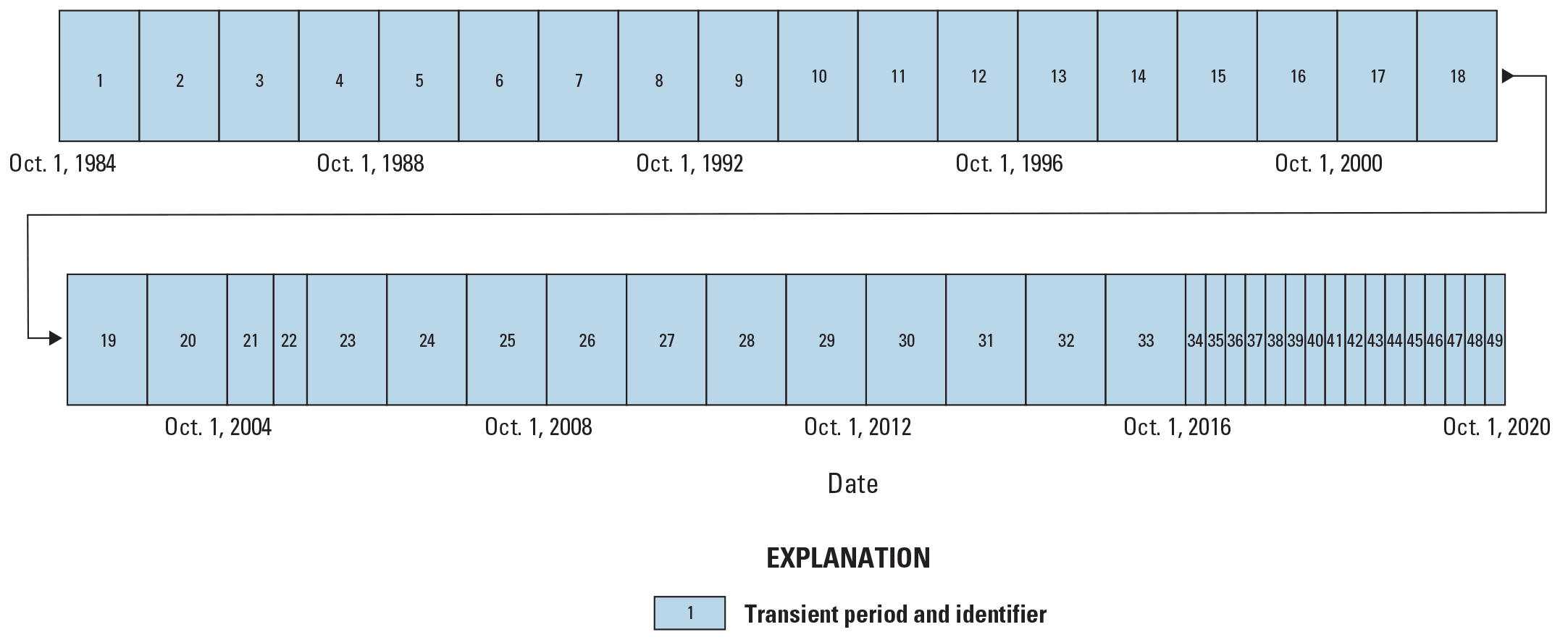
Periods and length of time covered by each of the 49 transient model stress periods.
Boundary Conditions
As noted above, the Badger model simulates groundwater flow in unconsolidated sediments and sedimentary bedrock. Hydraulic boundary conditions were applied to represent flows into and out of the model. The bottom boundary of the model is a no-flow boundary representing the contact between Paleozoic sedimentary bedrock and Precambrian crystalline bedrock units. The top boundary is a specified flux representing recharge to the groundwater system. The lateral boundary conditions are a combination of specified heads and specified fluxes extracted from a regional model for Columbia County (Gotkowitz and others, 2021) that are forced using the MODFLOW Well (WEL) package. These lateral boundaries are set far away from the former BAAP site and the identified plumes to minimize their effect on computed flow directions and rates.
Potential recharge to the groundwater system was applied to the surface of the model active area using estimates from the USGS Soil-Water-Balance (SWB) model (Westenbroek and others, 2018) for the area surrounding the former BAAP (Nielsen, 2023). The SWB model uses climate data and readily available spatial datasets of landscape and soil properties to calculate a Thornthwaite-Mather soil water balance on a daily time step and produce an estimate of net infiltration (also referred to as potential groundwater recharge) of water beneath the rooting zone. Potential groundwater recharge grids were estimated by the SWB model on a daily time step and aggregated to total potential recharge for every time step in the model simulation. The SWB model was also used to estimate the runoff from upland watersheds on the Baraboo Hills that seep into the subsurface through losing stream segments. This runoff was applied as recharge from stream segments near the base of the Baraboo Hills using the WEL package. The average annual simulated potential recharge for the model area from 2000 to 2020 is shown in figure 12 to illustrate the general pattern of recharge cross the site. Additional details on the SWB model development and results for the area near the former BAAP are in appendix 2 of this report, and model files are available in a model archive (Nielsen, 2023).
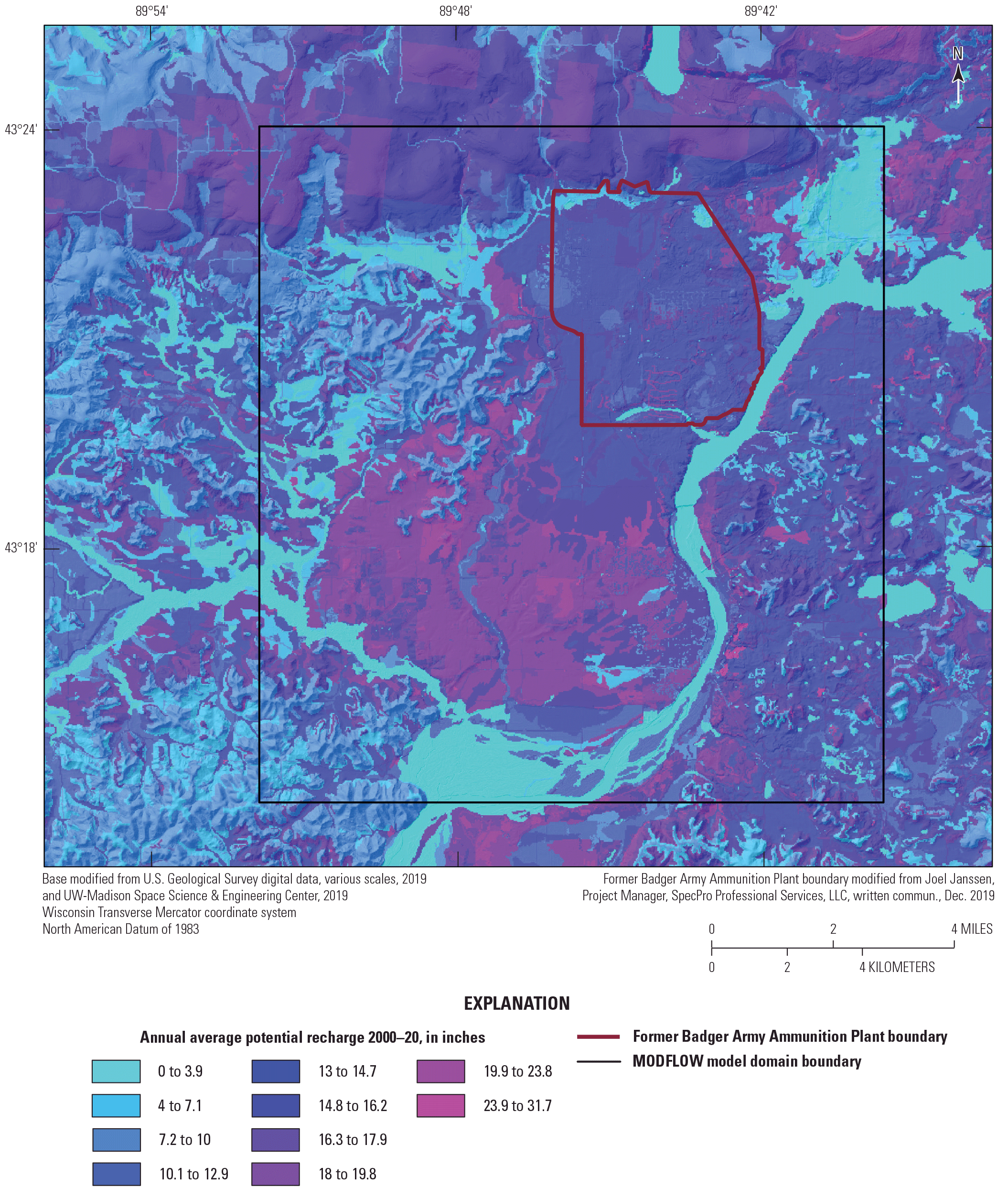
Average annual potential recharge simulated by the Soil-Water-Balance model for the study area, 2000–20.
The internal boundary conditions imposed on the Badger model (fig. 13) were represented using the following packages:
-
Groundwater withdrawals from permitted water use and site remediation pumping were simulated using 30 MODFLOW Multinode Wells (MNW2) package that allows removal of water from multiple MODFLOW layers from a single well.
-
Streams including Otter Creek were simulated as a head-dependent flux boundary condition using the MODFLOW Streamflow-Routing (SFR2) package.
-
Wetlands, small lakes, and ponds were simulated using the MODFLOW Drain (DRN) package.
-
The Wisconsin River was simulated using the MODFLOW River (RIV) package with five conductance zones.
Permitted groundwater withdrawals for municipal and irrigation wells in the model area were minimal and distant from the plumes so they were inherited as the steady-state pumping rates from the Columbia County groundwater flow model (Gotkowitz and others, 2021). Transient pumping from the interim remedial measure/MIRM pump-and-treat wells (Joel Janssen, Project Manager, SpecPro Professional Services, LLC, written commun., February 2, 2021) on the former BAAP site was also included. Minor withdrawals from private residential wells are not included because most of the water pumped from these wells is returned to the system through onsite septic, and the rates are typically small enough to not greatly affect groundwater flow directions.
The SFR2 package allows the model to estimate the stream stage and flux between the aquifer and the stream for Otter Creek and other smaller streams. In this model, streamflow represents base-flow conditions reflecting exchanges with the groundwater system and does not include stormflow components. The interaction between the stream and the aquifer is determined by (1) the stage in the stream relative to the groundwater elevation (hydraulic head) in the aquifer and (2) a conductance term based on the streambed dimensions and the vertical hydraulic conductivity (Kv) of the streambed sediment. Losses from the stream to the aquifer are controlled by the streamflow in that reach. The package was set up using the SFRmaker tool (Leaf, 2018) with hydrography information for this area from the National Hydrography Dataset Plus (McKay and others, 2012) and the land surface elevations from the light detection and ranging digital elevation model (USGS, 2019; University of Wisconsin–Madison, 2019a,b).
The RIV package is a head-dependent flux boundary condition based on the hydraulic head in the aquifer relative to a specified river elevation and a conductance term. River elevations were assigned using average water surface elevations above and below the hydroelectric dam with an assumed linear gradient in river surface downstream from the dam (water elevations in dataset provided by Amanda Blank, Site Manager, Hydroelectric & Gas Generation, Alliant Energy, written commun., December 29, 2020 [These data are not publicly available. Contact Alliant Energy for further information.]). The linear gradient was calculated using the average water elevation below the dam (starting at model row 288) and the light detection and ranging elevation at the outlet of Otter Creek, as used in the SFR2 package. The conductance of the riverbed depends on the model cell area, the thickness of the riverbed, and the Kv of the riverbed material. To account for sedimentation above the dam, which is thought to reduce the Kv, the conductance of the riverbed was divided into five zones: three representing the area upstream from the dam and two for the area downstream from the dam (fig. 13). Representing the Wisconsin River with the RIV package is less sophisticated than the SFR2 package but is reasonable because the river stage does not change much during the simulation. Trial simulations demonstrated that using the RIV package with fixed stage values can accurately represent the river as a discharge zone for regional flow as well as localized flow affects from the dam.
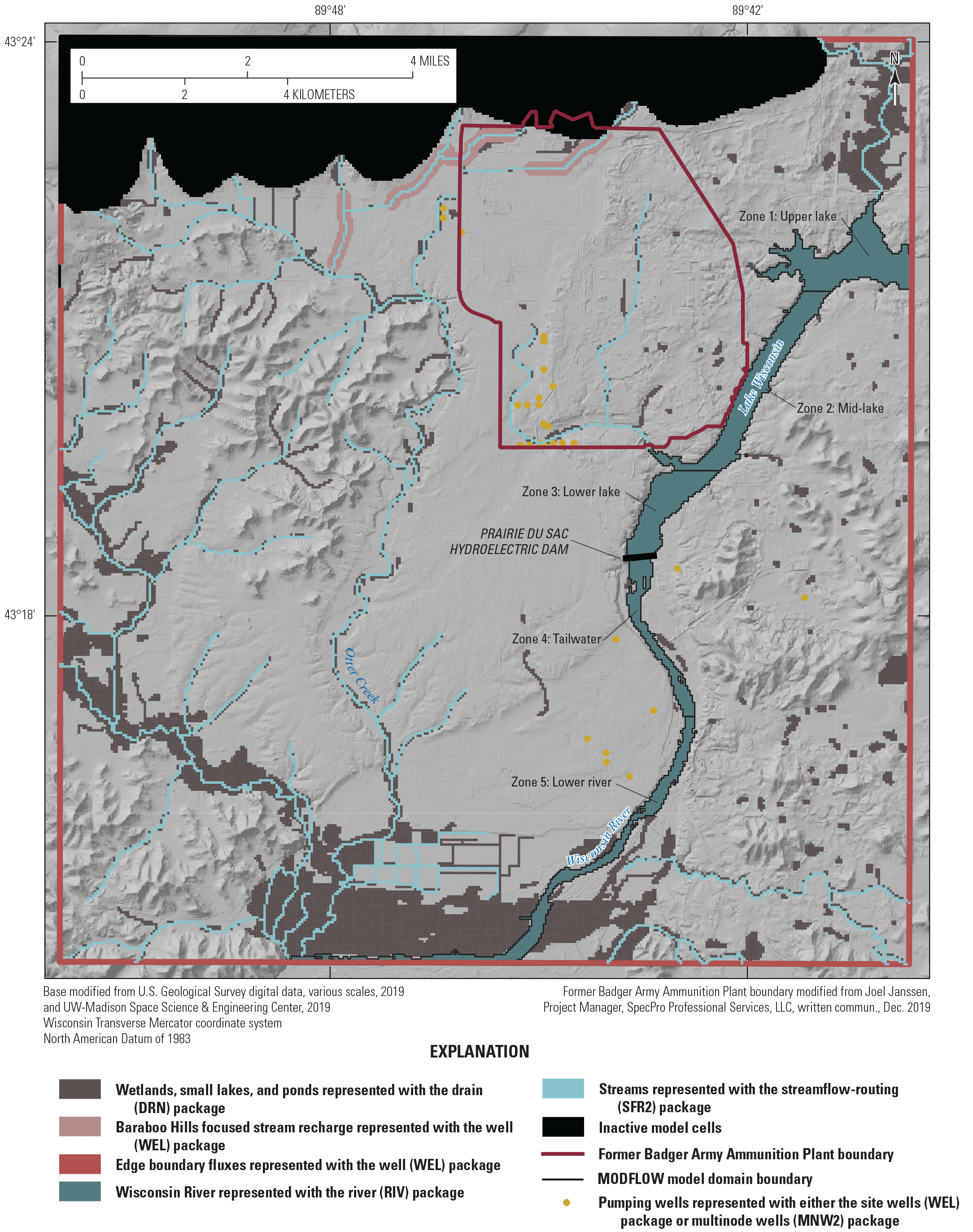
Internal boundary conditions for the model.
Aquifer Properties
Aquifer properties, including hydraulic conductivity (Kh and Kv), specific storage (Ss), and specific yield (Sy), were defined by the hydrostratigraphic zones from the unconsolidated hydrofacies for the upper 10 model layers and the mapped bedrock units for the lower 4 layers (see app. 3). Zone categories for the unconsolidated included gravel, sand and gravel, sand, mixed coarse, mixed fine, silt and clay, and clay. Zone categories for the bedrock layers included the upper bedrock unit, the Eau Claire Formation (including separate weathered zone), the Wonewoc Formation (including separate weathered zone), the Mount Simon Formation, and a zone representing the weathered upper bedrock and the Baraboo transition zone for the thin wedge of unconsolidated and bedrock material along the southern base of the Baraboo Hills. The Eau Claire and Wonewoc weathered units represent saprolitic zones near the top surface of the bedrock where weathering can give rise to enhanced hydraulic conductivity. Figure 14 shows the hydrostratigraphic units for the bedrock and unconsolidated material in the 14 model layers.
A starting value for the hydraulic conductivity, and lower and upper bounds on the value were assigned for each zone in the bedrock and unconsolidated materials. During model calibration (described in the next section), the assigned value and bounds were updated to give the model simulation results that better match observed behavior of the system.
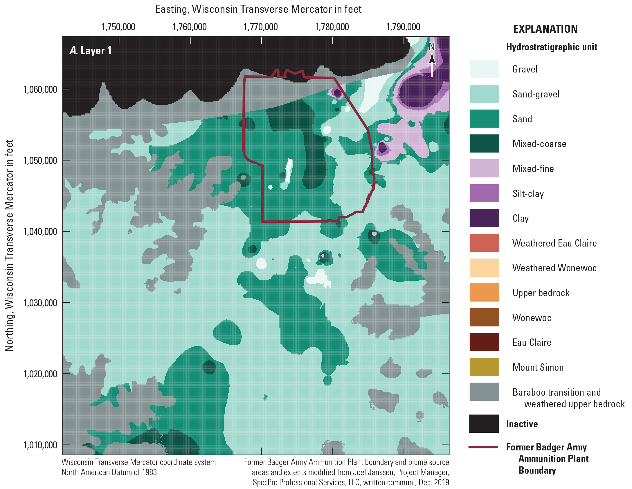
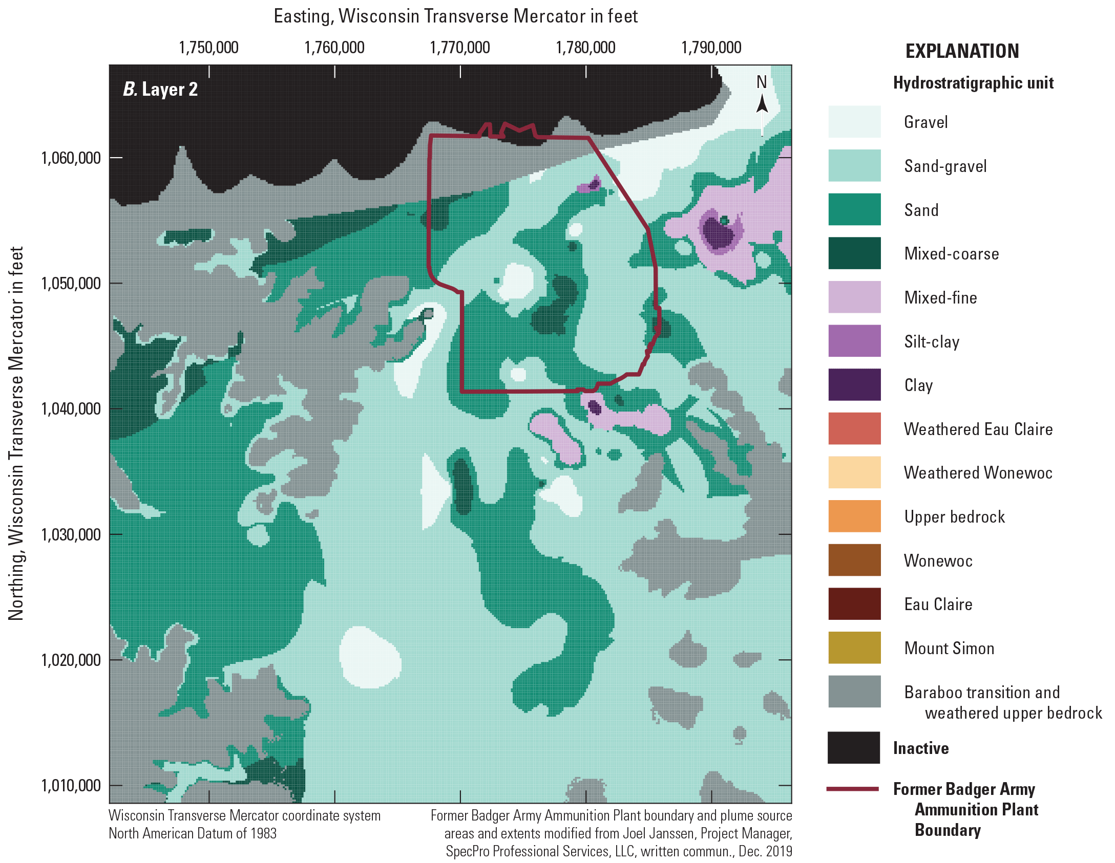
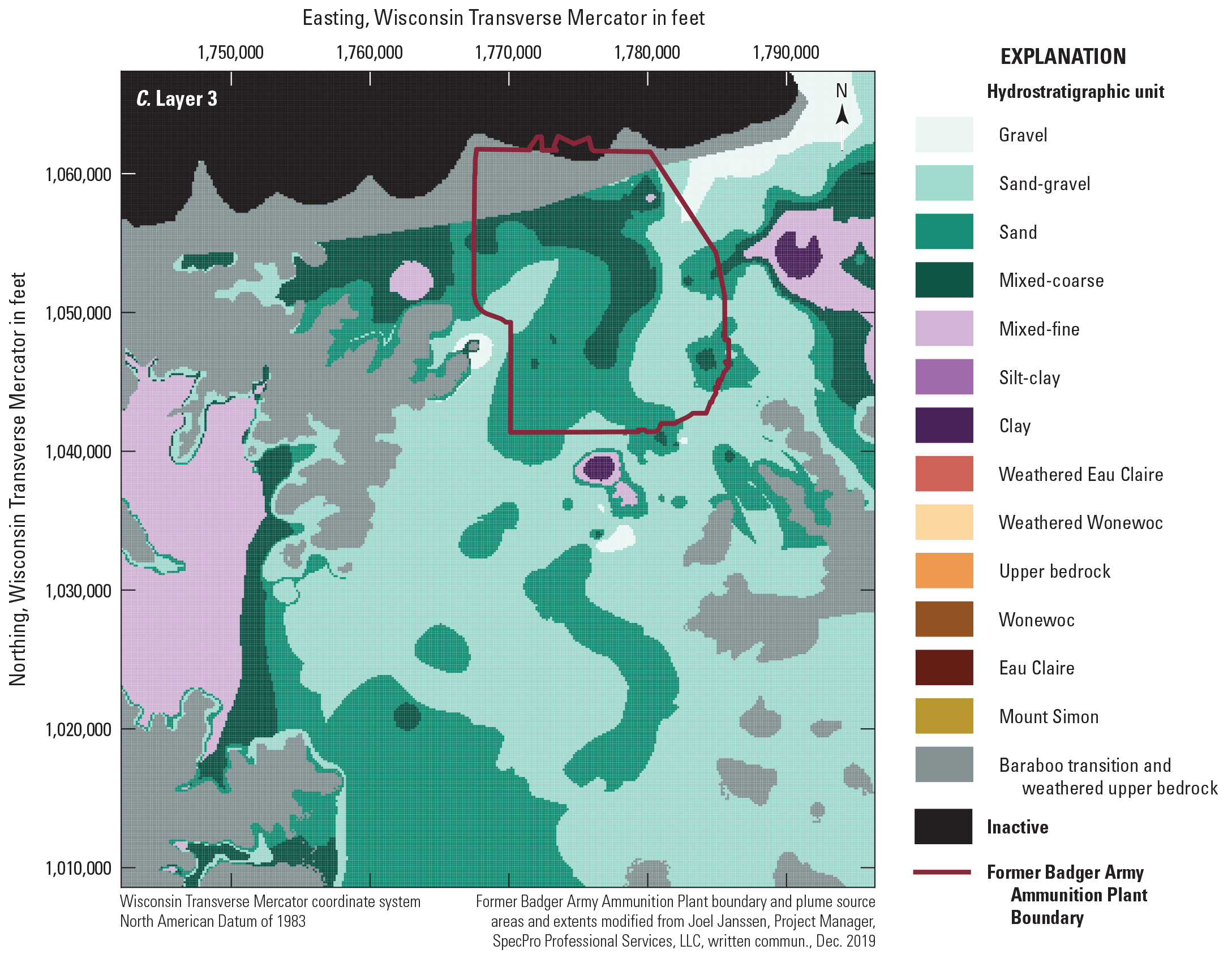
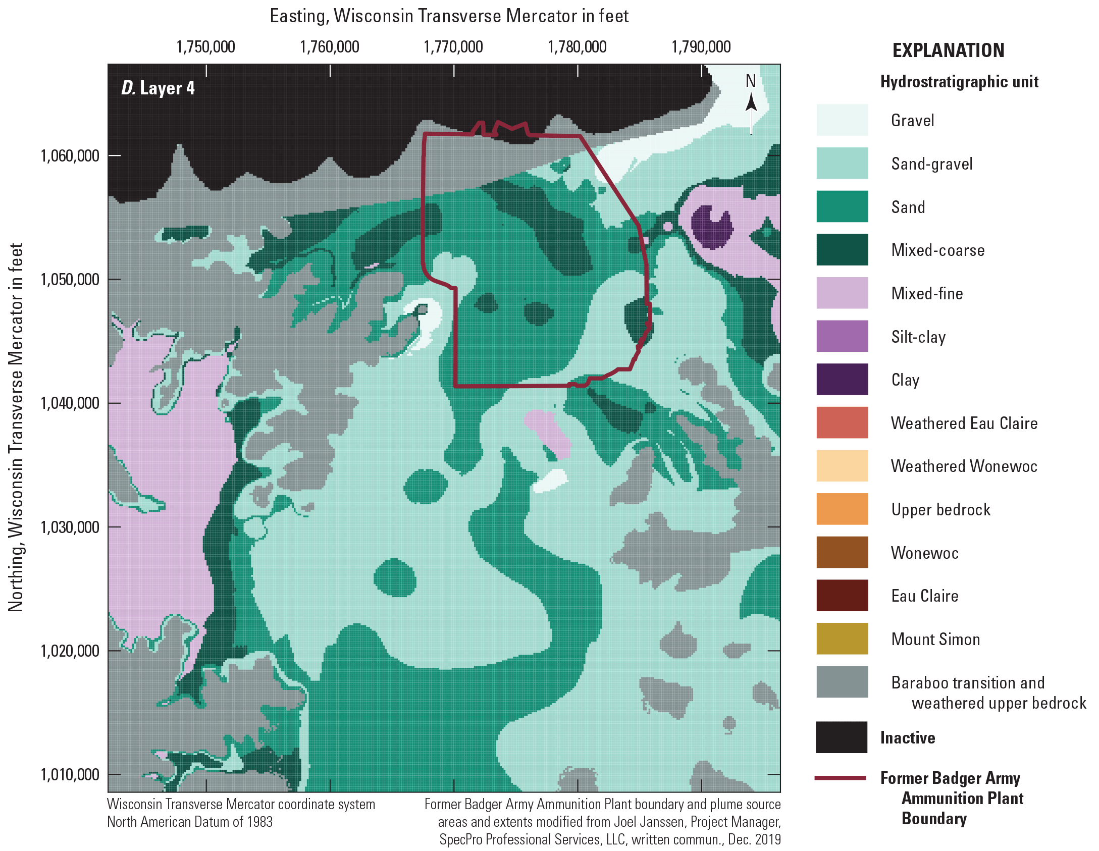
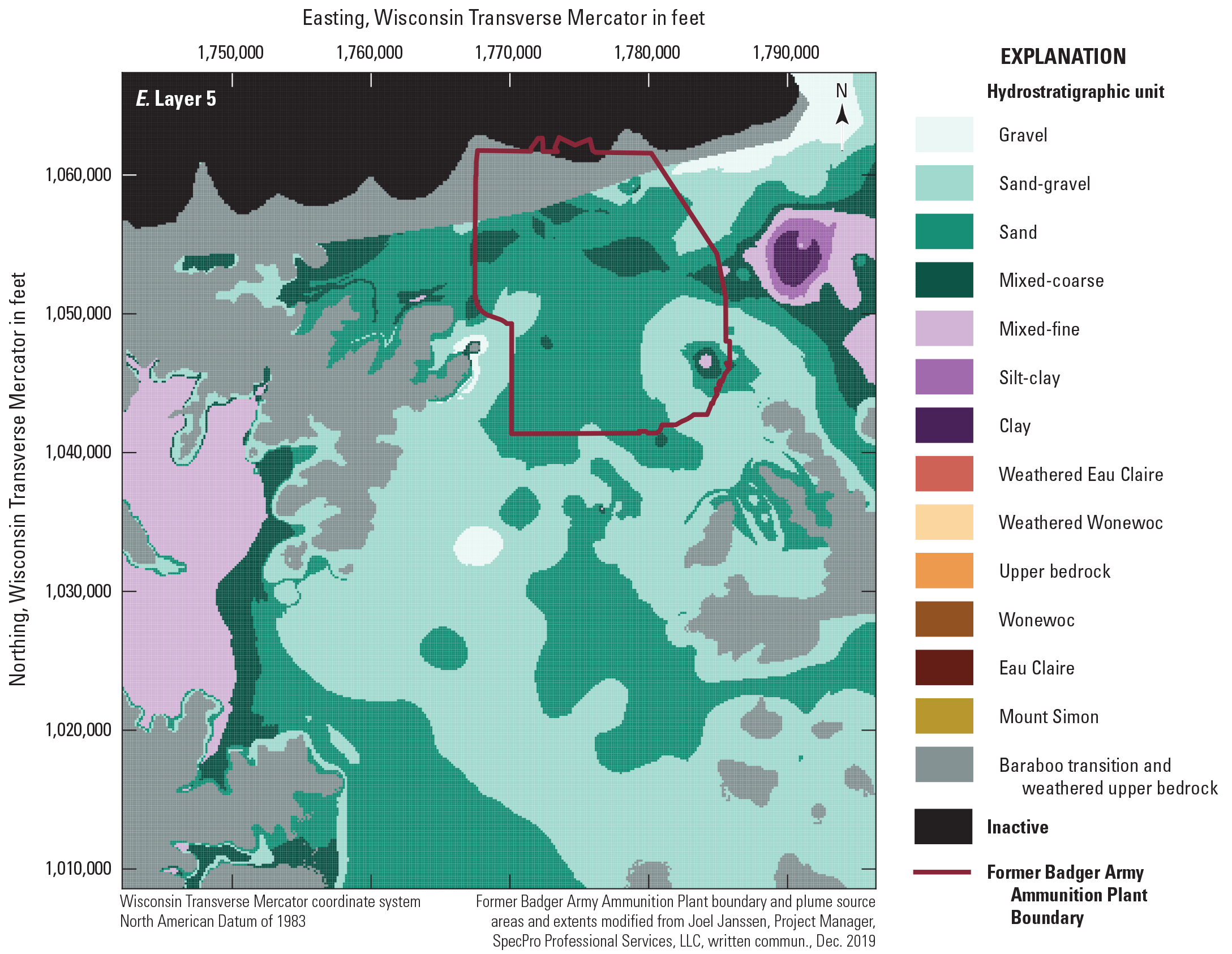
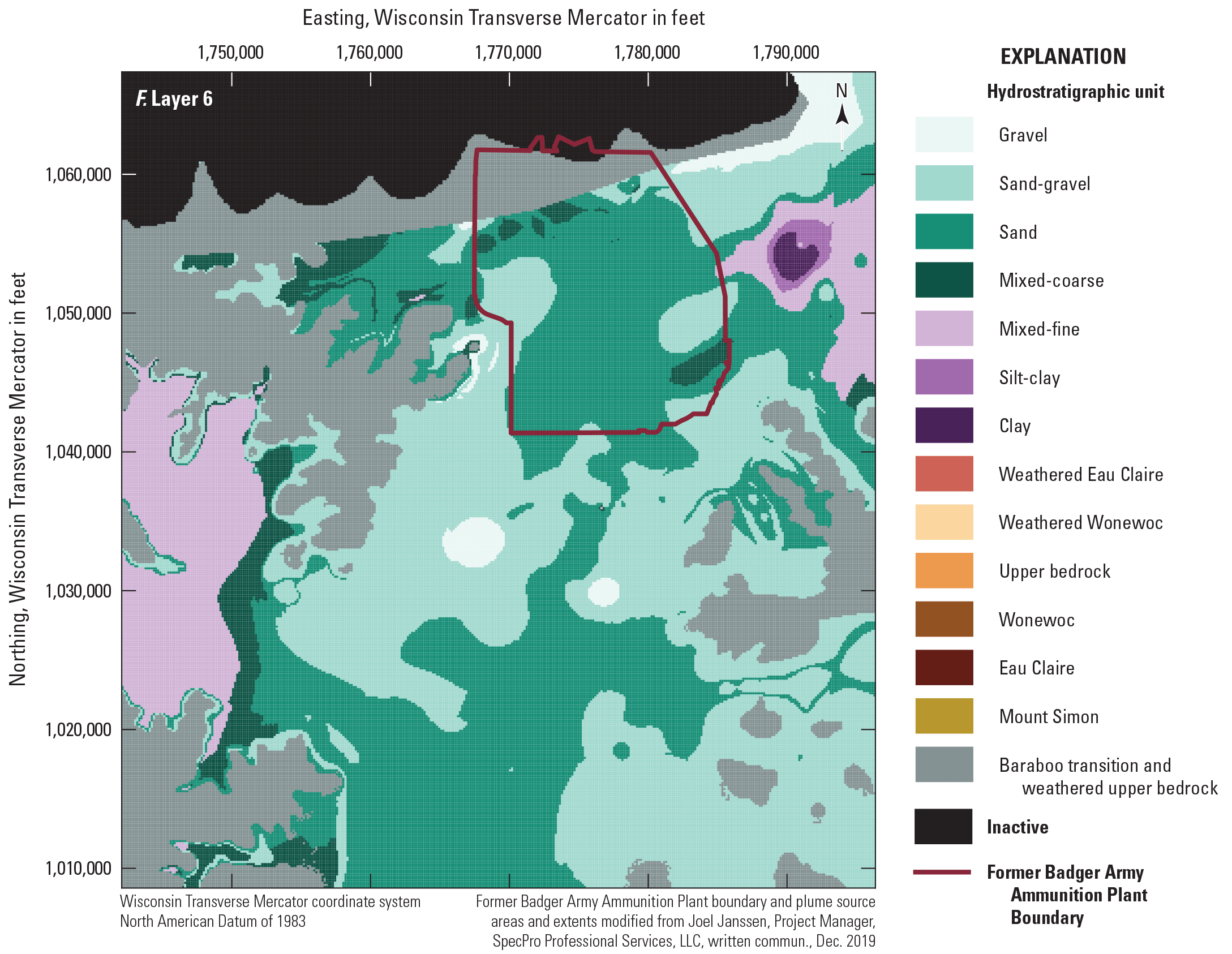
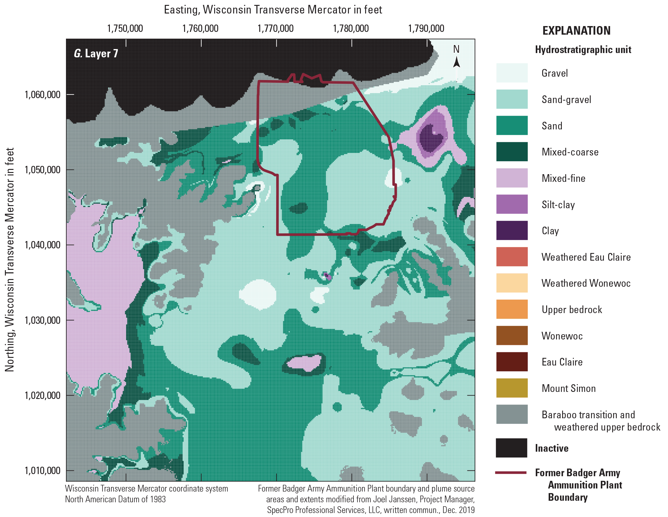

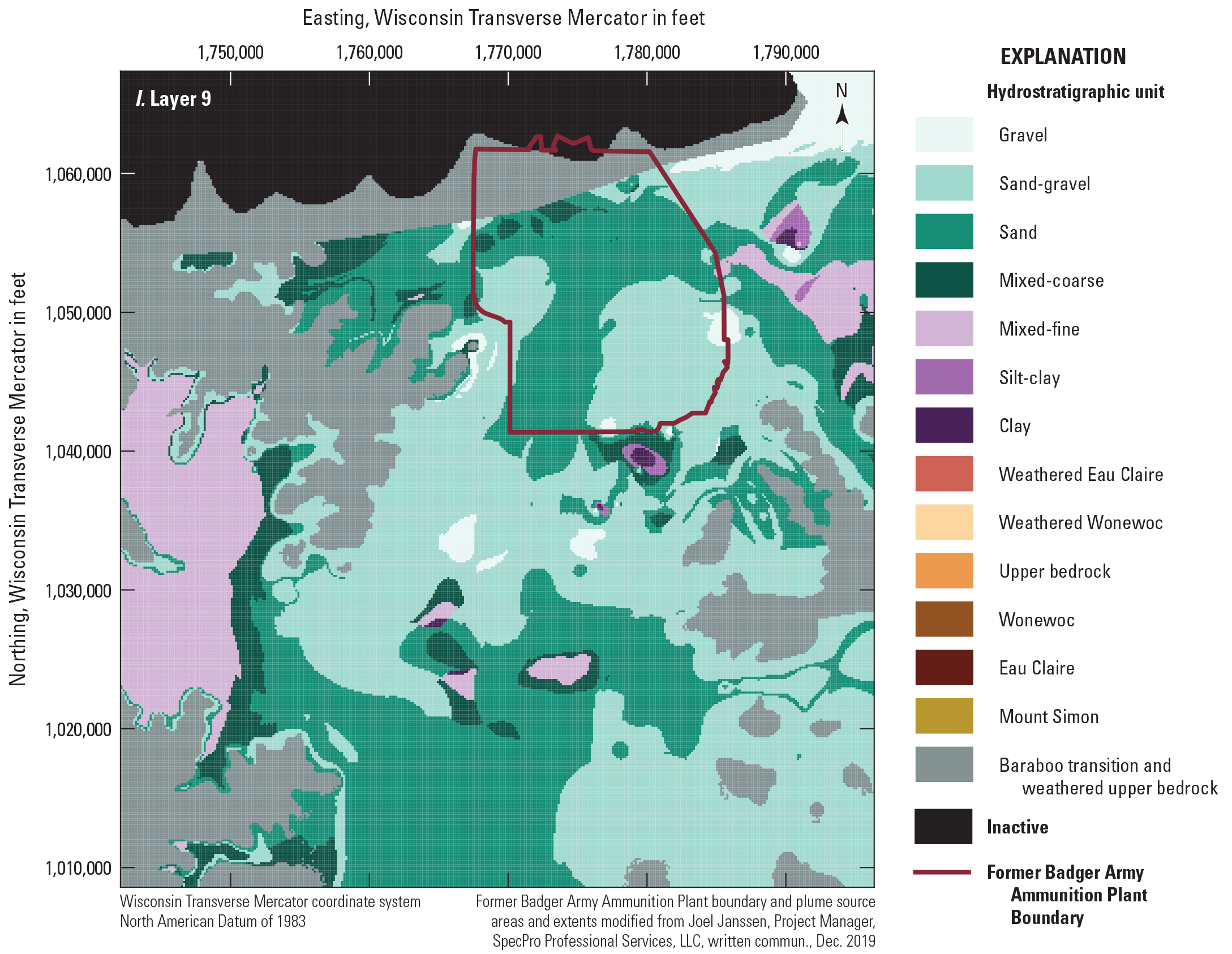

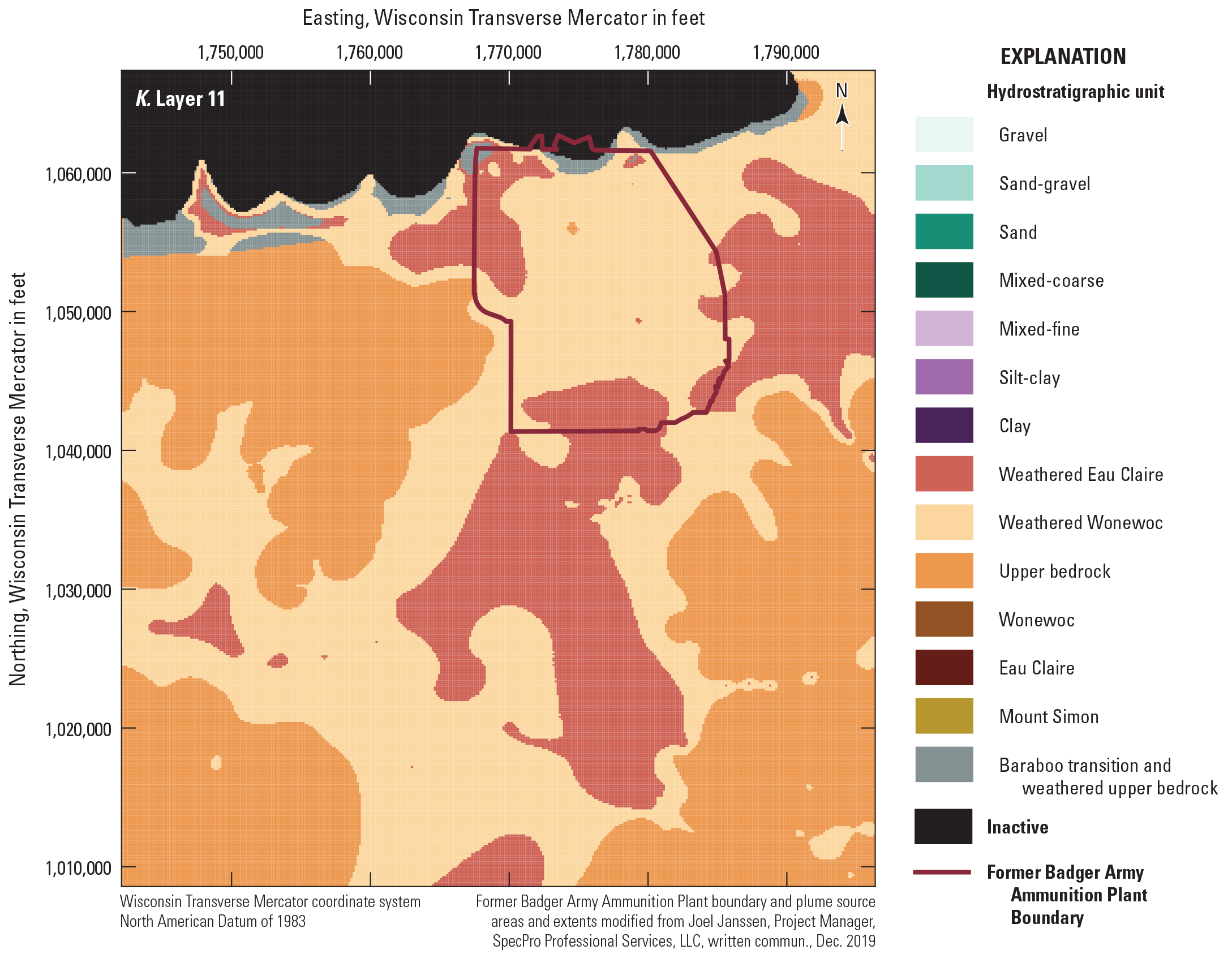
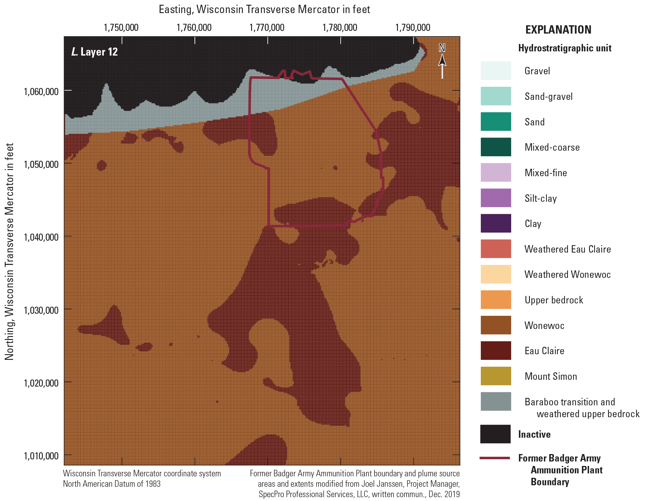
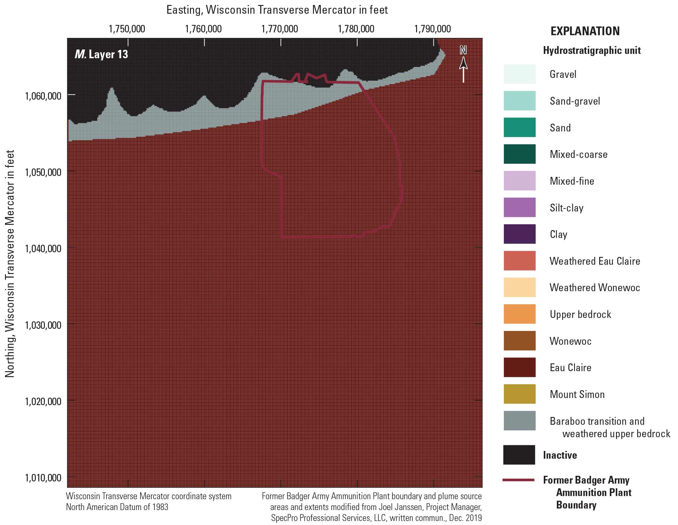
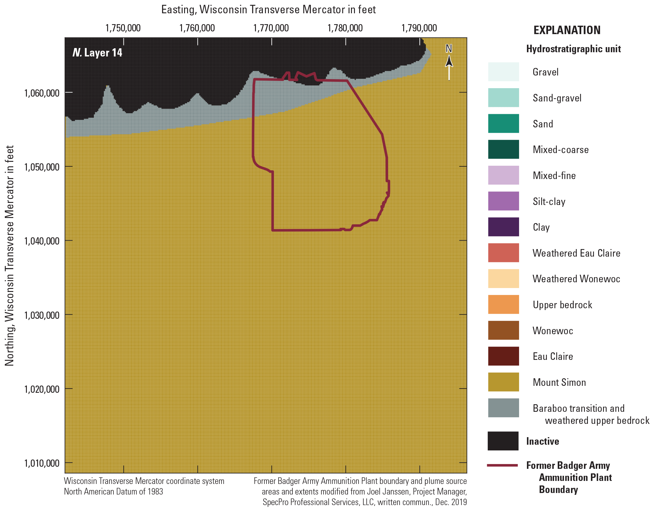
Hydrostratigraphic units for each of the 14 model layers.
Groundwater Flow Model Calibration
The Badger model required many inputs to define the model domain, aquifer characteristics, and boundary conditions necessary to simulate groundwater flow and advective transport of particles through the groundwater system using a MODPATH model. Some of these inputs are uncertain, and values for these are adjusted so that model simulation results better match observed values from the site. The uncertain values are referred to as model parameters in the following section; and this process is known as calibration, parameter estimation, inverse modeling, or history matching. This report uses the term calibration. Model calibration aims to reduce predictive uncertainty by adjusting model parameters until the modeled values acceptably match the observed values, without either overfitting to noise in the data or using geologically unreasonable values for model inputs (honoring prior information about the system). Historical observations used for the calibration included groundwater levels, streamflow, groundwater hydraulic gradients, and plume particle paths. The calibration was performed using the iterative ensemble smoother (iES) algorithm implemented in PEST++ (version 5.0.6, White, 2018; White and others, 2020). The computer program implementing this algorithm is called PESTPP–iES in this report.
The iES algorithm combines uncertainty estimation with parameter estimation to provide sets of input parameter values that are consistent with assumed uncertainty ranges for the parameters and assigned uncertainty in observations. An individual set of parameter values is called a realization, and all the realizations for the same iteration is called an ensemble. iES differs from other formal parameter estimation methods because it operates with ensembles rather than trying to determine a single “best fit” set of parameter values. An initial ensemble (prior) was generated by assigning hand-calibrated and literature values for the parameters of the Badger model and their ranges. PESTPP–iES generated 300 realizations assuming Gaussian distributions centered on each starting parameter value and spanning 4 standard deviations (assumed to represent the 95-percent confidence interval) set with the upper and lower parameter bounds. The MODFLOW–NWT and MODPATH models were then run with each parameter realization to provide a range of model outputs. PESTPP–iES then used empirical correlations between parameter and observation ensembles to produce an updated (posterior) ensemble of parameter realizations that should reduce parameter uncertainty and the discrepancy between model outputs and observations. This process was repeated for several iterations or until a desired fit between model outputs and observed values was produced. Experience with the algorithm indicates that the parameter ensembles after two or three iterations usually produce good fits to observations without overfitting (Hunt and others, 2021). The PESTPP–iES posterior parameter ensembles reflect the inherent uncertainty in the parameters and model and are conditioned on the available data. After iteration, this ensemble can then be used for predictive analysis—in this case, realizations from the calibrated flow model are being used in a future groundwater-transport model for the site.
Model Target Groups
Using groundwater level observations and streamflow measurements, 14 target sets were created to calibrate the Badger model. The sets and observation group names used in the PESTPP–iES calibration are detailed in appendix 4. A high number of target sets was designed to explore the many aspects of the model parameters (for example, aquifer properties, recharge, and conductance) using the site historical data, mostly water levels, measured at various locations, depths, and times. Of particular interest were target sets that helped constrain the flow field near the plumes such as the MODPATH particles in set 10. The different target sets were weighted based on the uncertainty in the observations and to balance group representation relative to the total starting calibration phi. In PESTPP–iES nomenclature, phi is the sum of the squared weighted residuals between the observed and modeled values for all the target groups and is what the calibration process seeks to minimize. Figure 15 shows the relative contribution of each of the target groups (described in detail in app. 4, table 4.1; search using the set numbers) as a percentage of the initial model phi. Full details of the observation weighting scheme used for calibration can be found in the flow model archive (Reeves and Corson-Dosch, 2023)
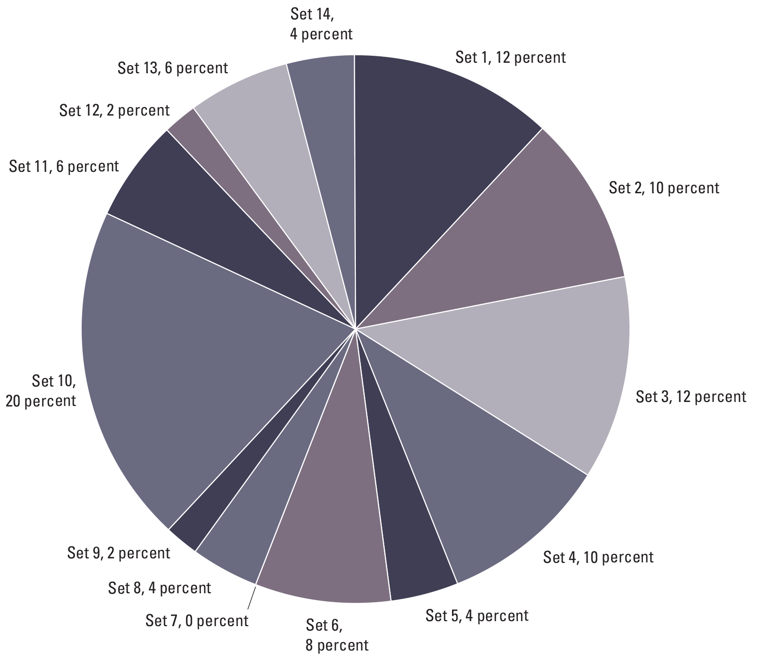
Percent contribution of each target group to the initial model phi.
Model Parameters
Model parameters include model inputs constrained to a range of values based on prior knowledge but are recognized as having some degree of uncertainty because of sparse measurement, measurement error, and structural errors inherent to the model (such as parameter simplification artifacts). Operationally, using multipliers as the adjustable parameters for the model has been efficient. The PESTPP–iES program is used to adjust the multipliers. In a preprocessing step, initial property values are multiplied by the multipliers to update model property values. The initial values were hand-adjusted before the PESTPP–iES calibration starting with values either inherited from the Columbia County model or from the literature. Most of the model parameters for the Badger model are pilot-point multipliers for hydraulic conductivity for the 14 hydrostratigraphic units (table 3). A pilot point is a specified location within a zone or unit where a value is adjusted; pilot points provide an estimate for the parameterized property that can change within the zone or unit. Other parameters include multipliers for recharge by zone, storage properties, and drain conductance. The only parameters that are not multipliers on initial values, but rather relate to values themselves, are parameters for the vertical anisotropy factor for hydraulic conductivity by zone, river conductance for five sections along the Wisconsin River, and porosity by model layer (table 3). The porosity parameters were not used in the flow model calibration.
Table 3.
Summary table of calibration parameter groups.[Data are summarized from Reeves and Corson-Dosch (2023)]
To simulate groundwater flow, hydraulic conductivity must be assigned for every finite-difference cell in the model. The hydrostratigraphic units (fig. 14) for the unconsolidated material and bedrock at the site discussed previously and detailed in appendix 3 were used to guide the initial estimates for Kh and Kv for the model. Some units only cover part of the model area and, thus, have few observations to inform how their properties vary spatially. For these units, a single hydraulic conductivity multiplier was used. Other units, like the sand, cover a large part of the model area and are expected to have variation in hydraulic conductivity within the unit. For these units, pilot points were used. Pilot-point parameters are multiplier values applied to initial hydraulic conductivity value at the locations shown in figure 16. The starting pilot-point multiplier values were 1, which maintains the original hydraulic conductivity field. The PEST groundwater utility FAC2REAL was used to interpolate from updated hydraulic conductivity estimates at the pilot points to a horizonal two-dimensional array of values for each finite-difference cell using kriging (Watermark Numerical Computing, 2020). PARM3D (Watermark Numerical Computing, 2020) was used to interpolate between model layers, and, in this case, assigned the same value for cells in the same hydraulic conductivity zone for all model layers at a given x-y location. For the Badger model, a grid of 1,254 evenly spaced pilot points was established (fig. 16), and the distance between the pilot points was 1,500 ft.
Distribution of pilot points across the Badger model domain.
The Kv was estimated by applying an anisotropy ratio (Kv:Kh) for the 14 hydrostratigraphic units. The anisotropy was uniform within each of the 14 units, so this parameter group had 14 parameters. The initial anisotropy assigned to most layers was 10 except for the Eau Claire unit, which was set to 100; and the weathered Wonewoc and Eau Claire units, which were set to 1.
The estimated recharge from the SWB model was considered uncertain and allowed to change by recharge zone. Appendix 2 describes the 16 recharge zones and the process used to determine an initial estimate for each zone. The updated recharge values are discussed in the Calibration Results section in this report.
Aquifer storage properties of specific storage and specific yield are needed for the transient model. However, data to constrain these properties are scarce, and the annual time spans for model stress periods also make it difficult to refine these properties in the calibration process. Therefore, only 6 aquifer storage parameters were used, and they are all multipliers against the initial values from Columbia County model: a single Ss and Sy for the unconsolidated units (z5–z11; table 3), a single Ss and Sy for the bedrock units (z1–z4; table 3), and a single Ss and Sy for the transitional and weathered bedrock units (z12–z14; table 3).
Wetlands and small ponds in the model area were simulated using the MODFLOW DRN package. A single multiplier for the drain conductance for each feature was assigned as a parameter. The Wisconsin River strongly affects the groundwater flow patterns in the model area. It was simulated in the model using the MODFLOW RIV package that requires river stage and riverbed conductance as inputs. The riverbed conductance was considered uncertain, and five zones (fig. 13) along the river were assigned different conductance parameters. The area immediately upstream from the Prairie du Sac hydroelectric dam was assumed to have the lowest riverbed conductance because the strong hydraulic gradient from the river towards the aquifer and lower water velocities could lead to more deposition of fines along the riverbed and, therefore, a lower hydraulic conductivity. Two other sections were imposed upstream from the dam: one section in the likely transition area where the hydraulic gradients switch from gaining to losing, and one section far upstream where the Wisconsin River is gaining and a higher initial value of riverbed conductance is assumed. One section was placed in the immediate tailwater of the dam where more turbulent flow likely flushed fine streambed material and the other was placed downstream from the tailwater section to represent normal streambed conditions. The parameters for these sections are direct riverbed conductance values passed to the groundwater flow model rather than multipliers.
Calibration Results
The model was considered calibrated when the modeled and observed hydraulic heads for the various target datasets were reasonably fit and particle tracks were consistent with observed plume boundaries. The iES algorithm seeks to minimize the squared weighted residuals between model outputs and observed values for an ensemble of objective function values that changes from iteration to iteration (fig. 17). In figure 17, the red curve represents a “base” ensemble member (defined in the next paragraph) that is taken as representative when a single realization is desired. The results of the third iES iteration was selected as optimal based on a subjective judgement that the objective function had lowered to an acceptable level of fit while not overfitting; that is, the ensemble retained some variability and captured important uncertainty in the system.
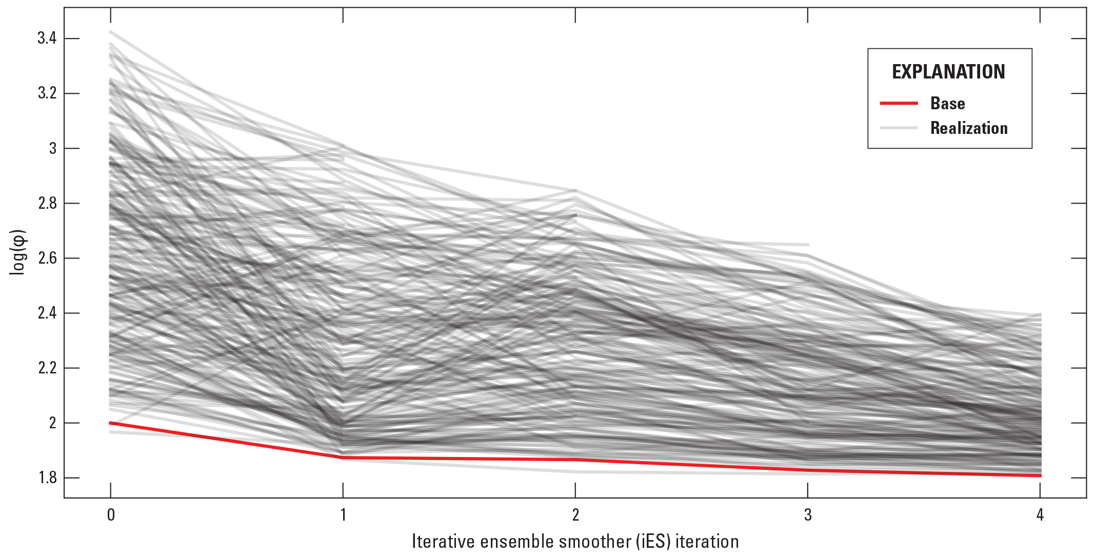
Summary of ensemble and base objective function progress by iterative ensemble smoother iteration.
For calibration results in this report, the range of results are presented for the full ensemble suite of successful runs, where applicable, and for the final “base” realization, where a singular model result is necessary. PESTPP–iES can experience failed model runs because of the randomized way parameter sets are generated; and when a run from the ensemble fails to converge, PESTPP–iES drops that run from the ensemble. In the model results shown, nearly 100 runs failed after 3 iterations, and the iteration 3 ensemble of results has 202 realizations. The final values of the “base” realization represent the central tendency of the parameter distribution at each calibration iteration (White and others, 2020). The base realization differs from the other realizations that are obtained by making a stochastic sample using the bounds of the initial parameter values. Instead, the base realization initially consists of the specific starting values provided to PESTPP–iES, which are considered “most likely” by the users. These “base” values are then adjusted during each iteration of the iES algorithm, but the central tendency typically remains, and this single realization typically is less variable than the other realizations (White and others, 2020). This section presents the representative base realization model (“base model”) properties, including hydraulic conductivities and boundary conditions that are representative of the optimal iES ensemble. This section also includes discussion of model results that were simulated using base realization parameters, including the simulated groundwater mass balance, water table, and streamflow. For the analysis of plume particle tracks, however, the entire ensemble of successful runs from iteration 3 was used to ensure that the range of outcomes, consistent with prior knowledge of the parameters and information from the observation data, were explored.
Aquifer Properties
Kh and Kv arrays for each of the 14 model layers are shown in figures 18 and 19 and presented in tables 4 and 5 for the base model, respectively. Figure 20 summarizes the Kh values for the full iteration 3 ensemble. Model Kh values generally agreed with the literature ranges from the Columbia County (Gotkowitz and others, 2021) and Sauk County (Gotkowitz and others, 2005) hydrogeology publications as well as the study slug tests. The base model unconsolidated Kh ranged from 2.6 to 547 ft/d and increased with increasing particles size of the sediment (that is, clay was lowest, and sands and gravels were highest). Bedrock had lower Kh than the unconsolidated materials, except for the clay and silt. The full range of Kh values for the aquifer property zones are summarized in table 4.
The mean vertical anisotropy (mean Kh ÷ mean Kv) for each of the aquifer property zones is presented with the Kv values in table 5. In general, Kh is expected to exceed Kv in sediments and sedimentary rocks where depositional bedding should allow for preferential flow in the horizontal direction (assuming bedding planes are still oriented close to their original deposition position). Typically, in groundwater flow models glacial sediments and sedimentary bedrock are assumed to have an anisotropy of around 10; for the base model, the anisotropy was generally between 6 and 14. Exceptions were the Eau Claire and weathered Wonewoc zones (anisotropy of 1) and the unweathered Eau Claire zones (anisotropy of 100). These values are consistent with the starting values used for these parameters. Weathering could introduce more vertical connectivity through fractures, thereby making the Kv and Kh more similar. In the unweathered Eau Claire Formation, the higher anisotropy could be attributed to the preferential horizontal flow from finer grained layers; Duffield (2019) notes anisotropy ratios can approach 100 when clay layers are present.
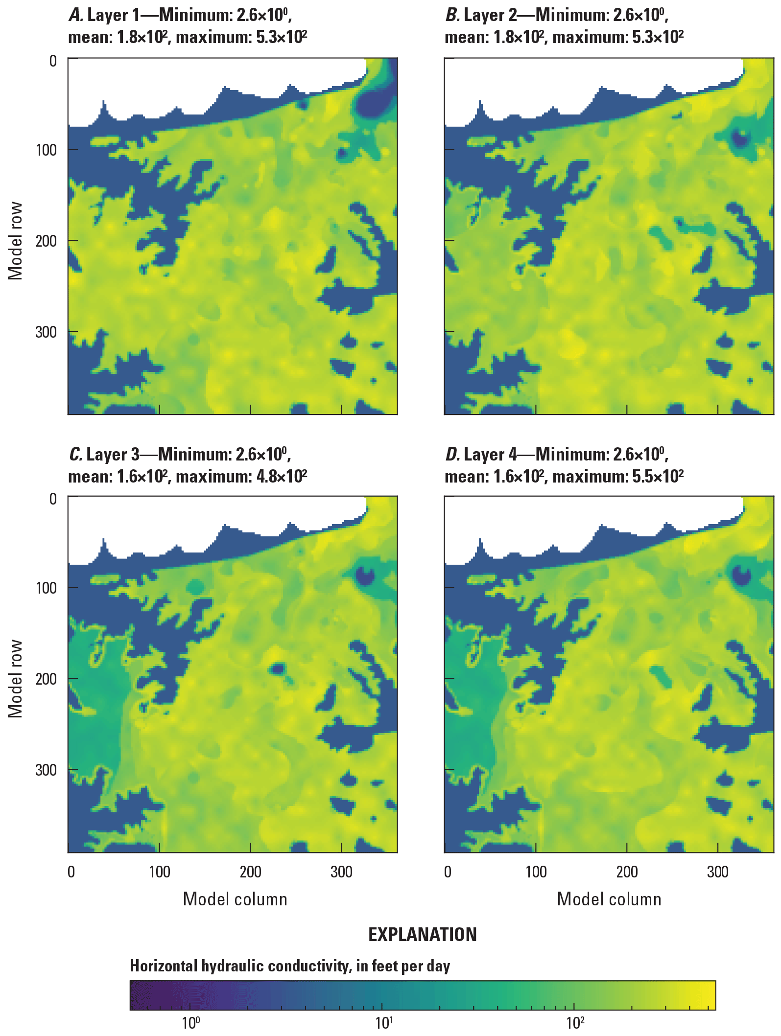
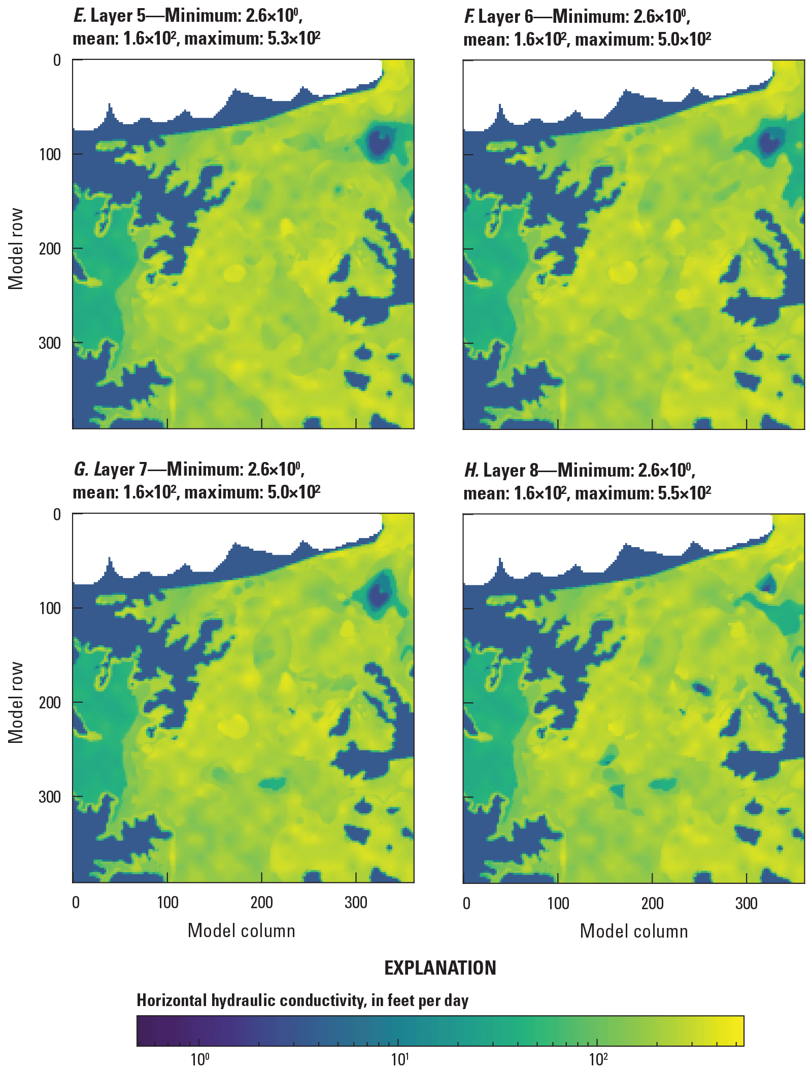
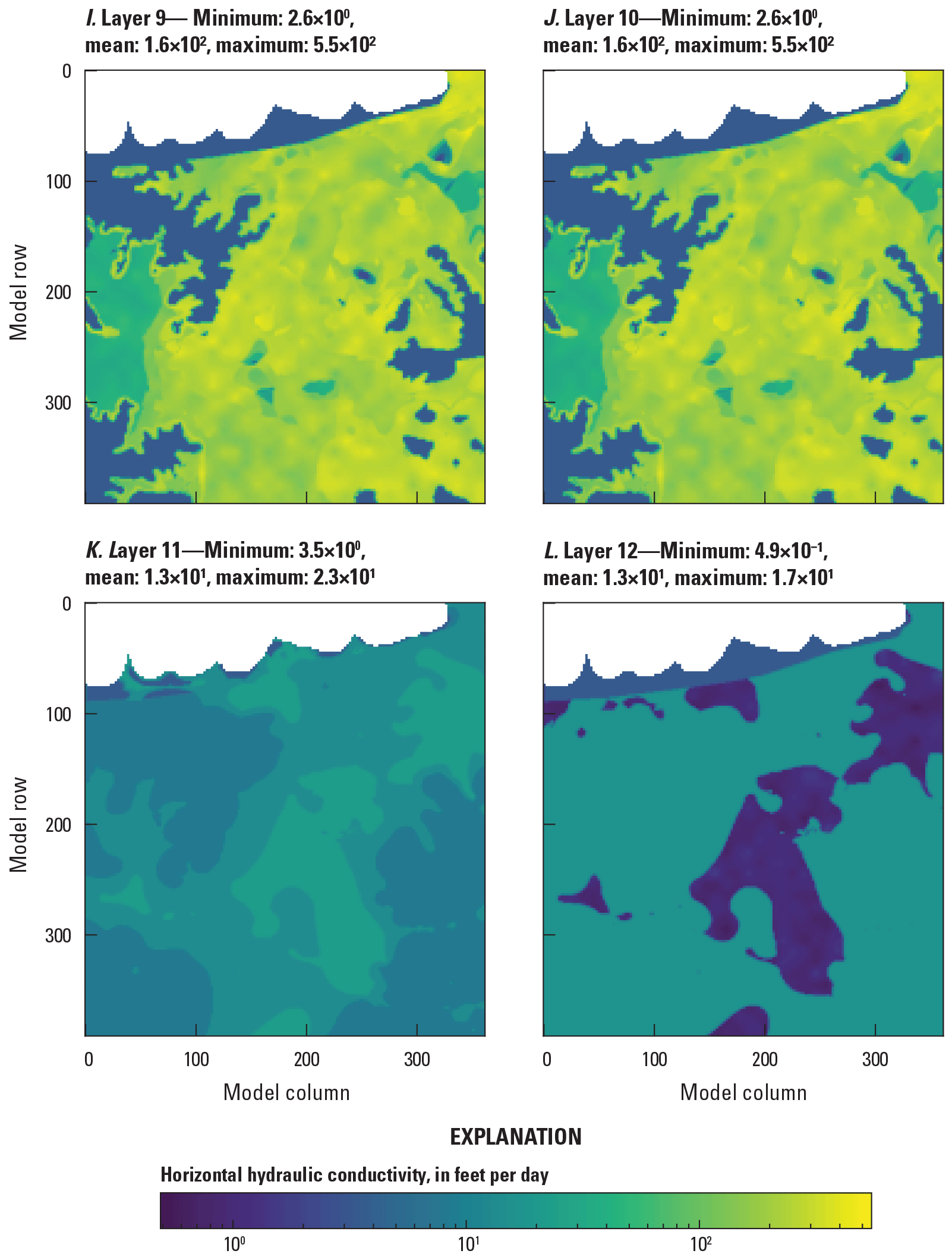
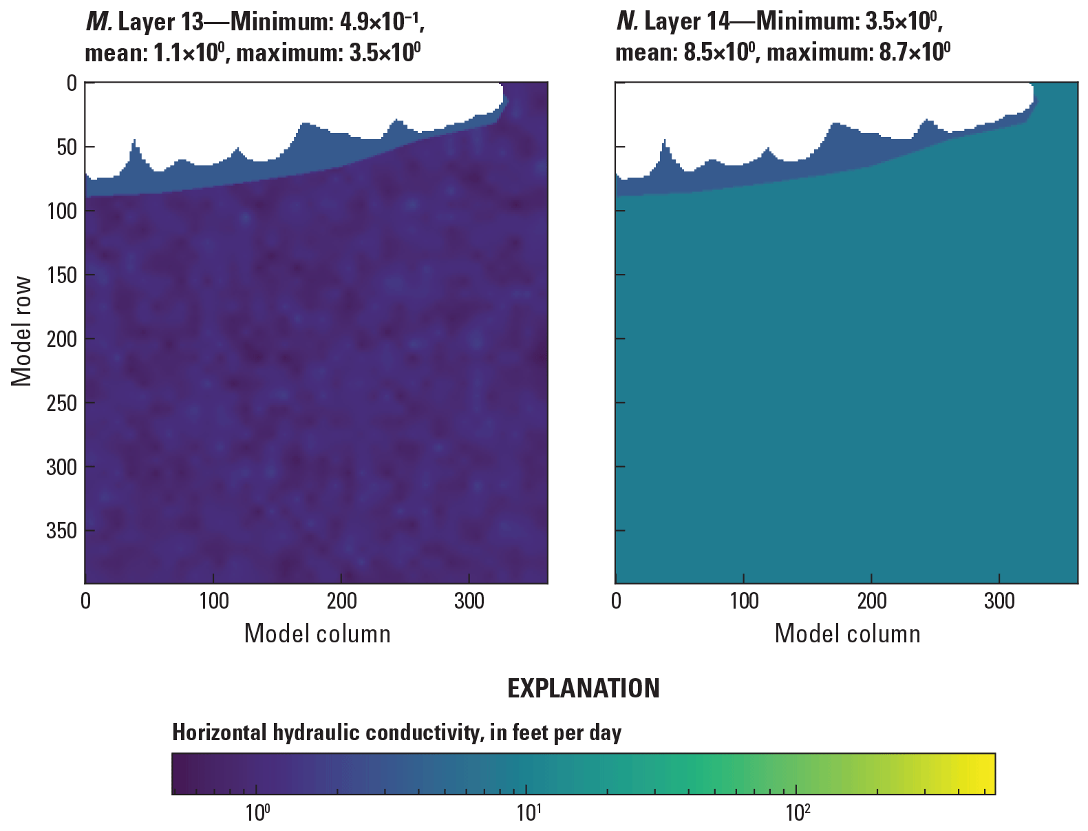
Horizontal hydraulic conductivity in each of the 14 model layers for the base groundwater flow model.
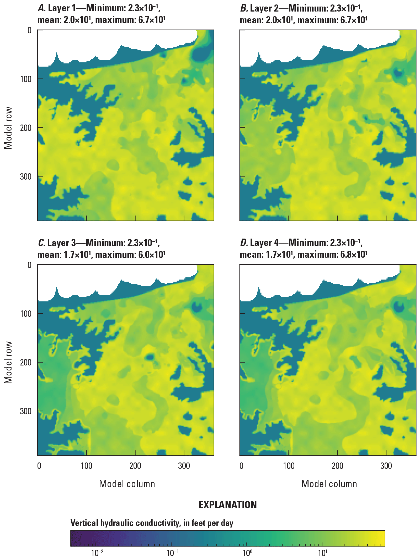
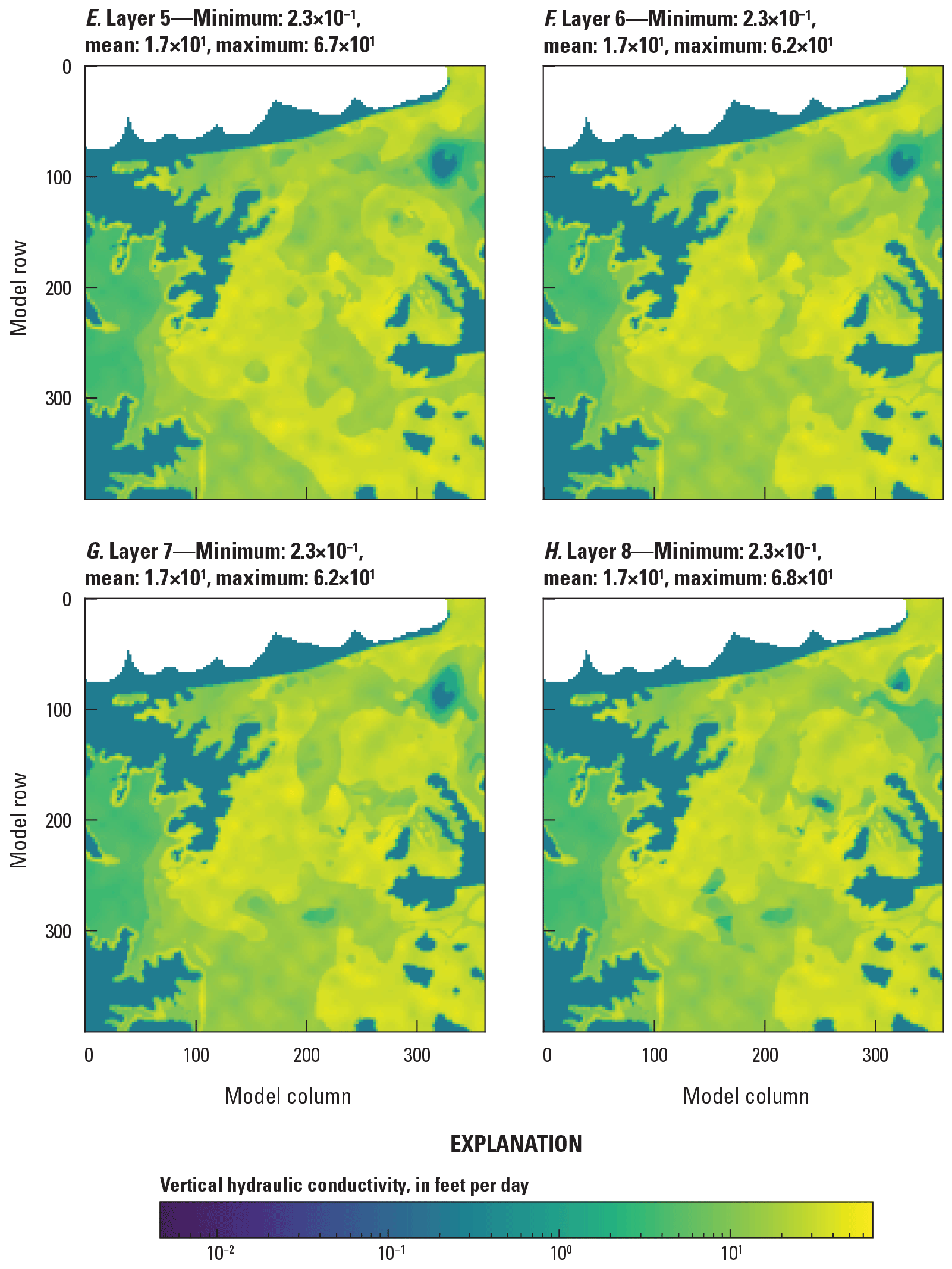
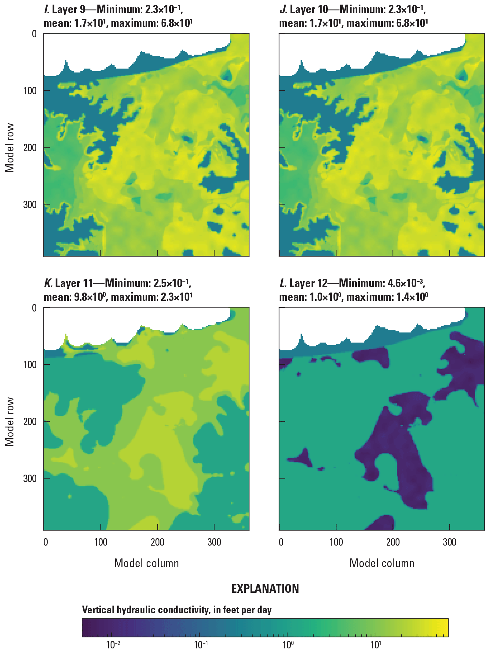
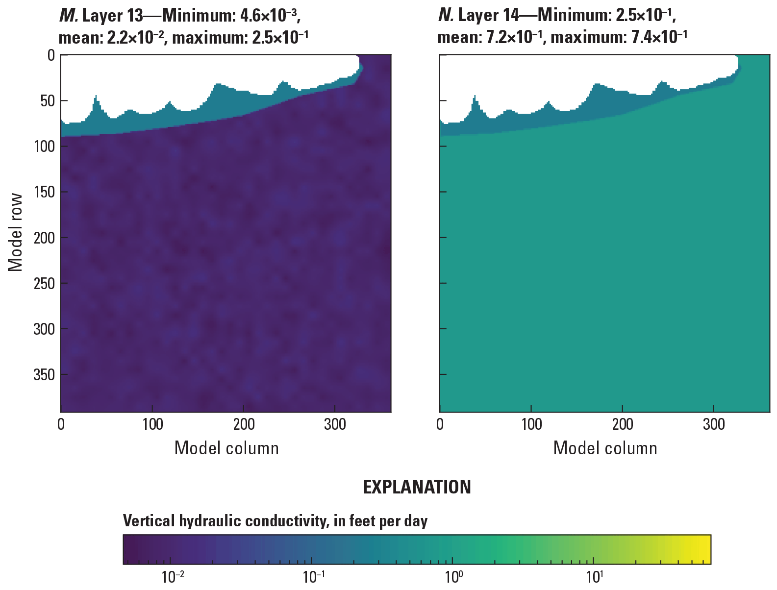
Vertical hydraulic conductivity in each of the 14 model layers for the base groundwater flow model.
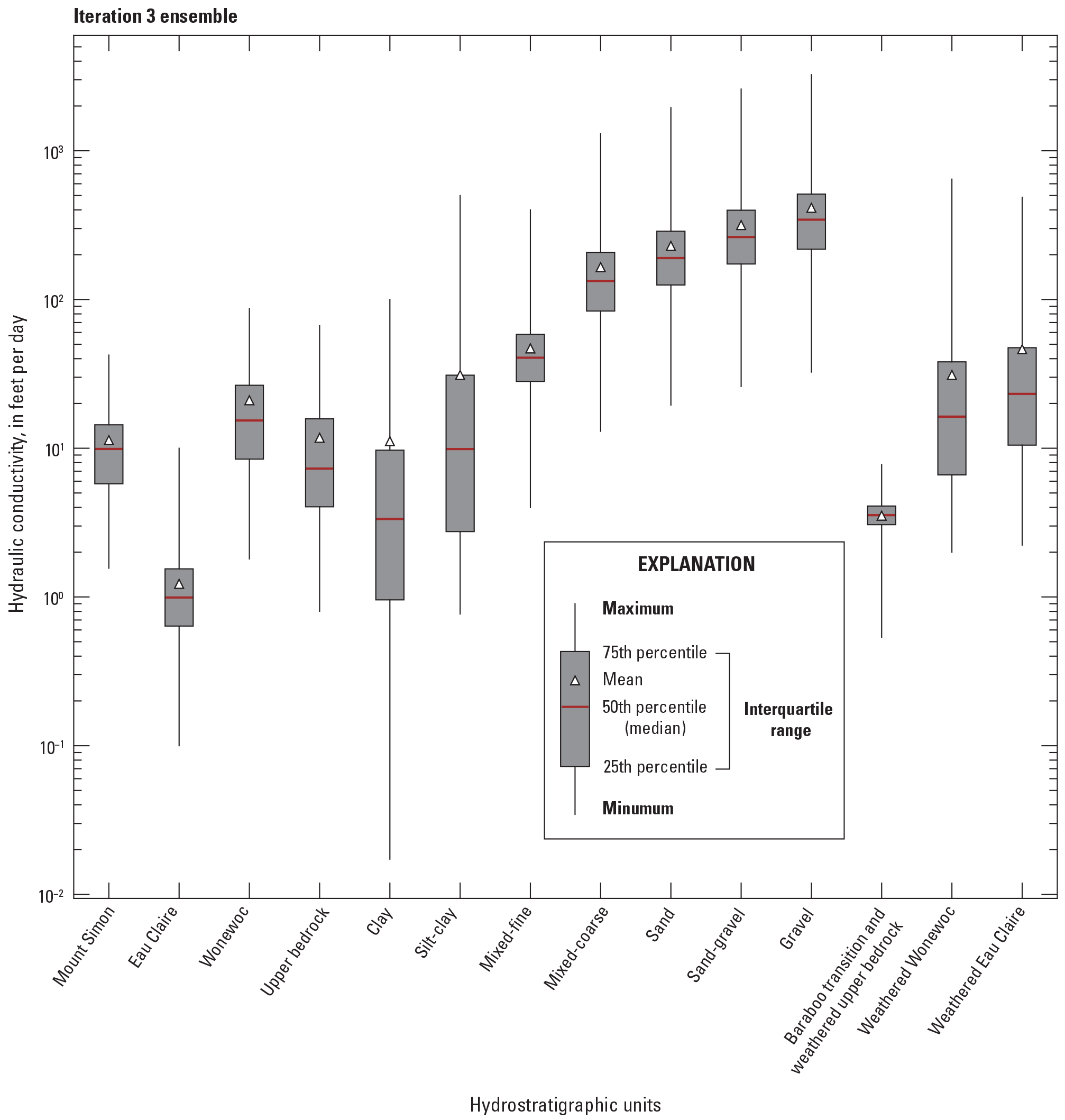
Horizontal hydraulic conductivity in each of the hydrostratigraphic units for the iteration 3 ensemble.
Table 4.
Summary table of calibrated horizontal hydraulic conductivity values and literature ranges for the hydrostratigraphic units in the base model.[Except where other sources are cited, data are summarized from Reeves and Corson-Dosch (2023). ft/d, foot per day]
| Hydrostratigraphic unit (app. 3) | Horizontal hydraulic conductivity, in feet per day | |||||
|---|---|---|---|---|---|---|
| Mean | Median | Maximum | Minimum | Literature ranges and sources | Study slug tests | |
| Clay | 2.6 | 2.6 | 2.6 | 2.6 | Sauk County unlithified aquifer 55–976 ft/d (specific capacity tests; Gotkowitz and others, 2005); Columbia County unlithified aquifer 1–910 ft/d (specific capacity tests; Gotkowitz and others, 2021) | Unconsolidated: 4.7–2,227 ft/d |
| Silt-clay | 10.3 | 10.3 | 10.3 | 10.3 | ||
| Mixed-fine | 41.0 | 40.5 | 102.3 | 20.3 | ||
| Mixed-coarse | 132.7 | 132.0 | 216.9 | 68.5 | ||
| Sand | 193.2 | 191.6 | 452.8 | 82.3 | ||
| Sand-gravel | 264.9 | 262.0 | 547.2 | 120.4 | ||
| Gravel | 338.9 | 341.6 | 525.9 | 233.5 | ||
| Baraboo transition and weathered upper bedrock | 3.5 | 3.5 | 3.5 | 3.5 | No literature for the deposits along the Baraboo Hills but should be similar to other unconsolidated material. Weathered upper bedrock should be within the upper bedrock range. | Not applicable. |
| Upper bedrock | 8.0 | 8.0 | 8.0 | 8.0 | Upper bedrock (above the Wonewoc) in Columbia County 0.2–200 ft/d with geometric mean of 2.4 ft/day (specific capacity tests; Gotkowitz and others, 2021) | Bedrock: 0.17–5.5 ft/d |
| Weathered Wonewoc | 14.1 | 14.1 | 14.1 | 14.1 | Modeling zone, should be within range listed for the Wonewoc. | |
| Wonewoc | 16.8 | 16.8 | 16.8 | 16.8 | Wonewoc Formation in Columbia County 0.2–1,072 ft/d with geometric mean of 5.7 ft/d (specific capacity tests; Gotkowitz and others, 2021) | |
| Weathered Eau Claire | 22.8 | 22.8 | 22.8 | 22.8 | Modeling zone, should be within range listed for the Eau Claire. | |
| Eau Claire | 1.0 | 1.0 | 2.3 | 0.5 | Eau Claire Formation in Columbia County 0.3–749 ft/d with geometric mean of 6.7 ft/d (specific capacity tests; Gotkowitz and others, 2021); Eau Claire 6´10−4 (vertical) in Dane County model (Krohelski and others (2000) | |
| Mount Simon | 8.7 | 8.7 | 8.7 | 8.7 | Mount Simon Formation in Columbia County 0.3–558 ft/d with geometric mean of 4.8 ft/d (specific capacity tests; Gotkowitz and others, 2021) | |
Table 5.
Summary table of calibrated vertical hydraulic conductivity and mean anisotropy for the hydrostratigraphic units in the base model.[Data are summarized from Reeves and Corson-Dosch (2023)]
| Hydrostratigraphic unit (app. 3) | Vertical hydraulic conductivity, in feet per day | Vertical anisotropy of mean horizontal hydraulic conductivity/mean vertical hydraulic conductivity, unitless | |||
|---|---|---|---|---|---|
| Mean | Median | Maximum | Minimum | ||
| Clay | 0.2 | 0.2 | 0.2 | 0.2 | 11 |
| Silt-clay | 1.3 | 1.3 | 1.3 | 1.3 | 8 |
| Mixed-fine | 4.2 | 4.2 | 10.6 | 2.1 | 10 |
| Mixed-coarse | 10.3 | 10.2 | 16.8 | 5.3 | 13 |
| Sand | 15.9 | 15.8 | 37.3 | 6.8 | 12 |
| Sand-gravel | 33.0 | 32.7 | 68.2 | 15.0 | 8 |
| Gravel | 27.3 | 27.5 | 42.3 | 18.8 | 12 |
| Baraboo transition and weathered upper bedrock | 0.2 | 0.2 | 0.2 | 0.2 | 14 |
| Upper bedrock | 1.2 | 1.2 | 1.2 | 1.2 | 6 |
| Weathered Wonewoc | 11.7 | 11.7 | 11.7 | 11.7 | 1 |
| Wonewoc | 1.4 | 1.4 | 1.4 | 1.4 | 12 |
| Weathered Eau Claire | 23.1 | 23.1 | 23.1 | 23.1 | 1 |
| Eau Claire | 0.010 | 0.009 | 0.022 | 0.005 | 105 |
| Mount Simon | 0.7 | 0.7 | 0.7 | 0.7 | 12 |
The Sy and Ss for the unconsolidated and bedrock units are shown in figures 21 and 22 and summarized in tables 6 and 7, respectively. Fewer calibration data were available to constrain Sy and Ss; all bedrock layers had the same value; and all unconsolidated layers shared the same distribution. The model Sy for unconsolidated material was on the upper end of literature values for these sediment types in table 6; the bedrock was on the lower end of literature bedrock values in table 6. For Ss, the simulated unconsolidated and bedrock values were on the lower end or slightly below the literature ranges for comparable materials in table 7.
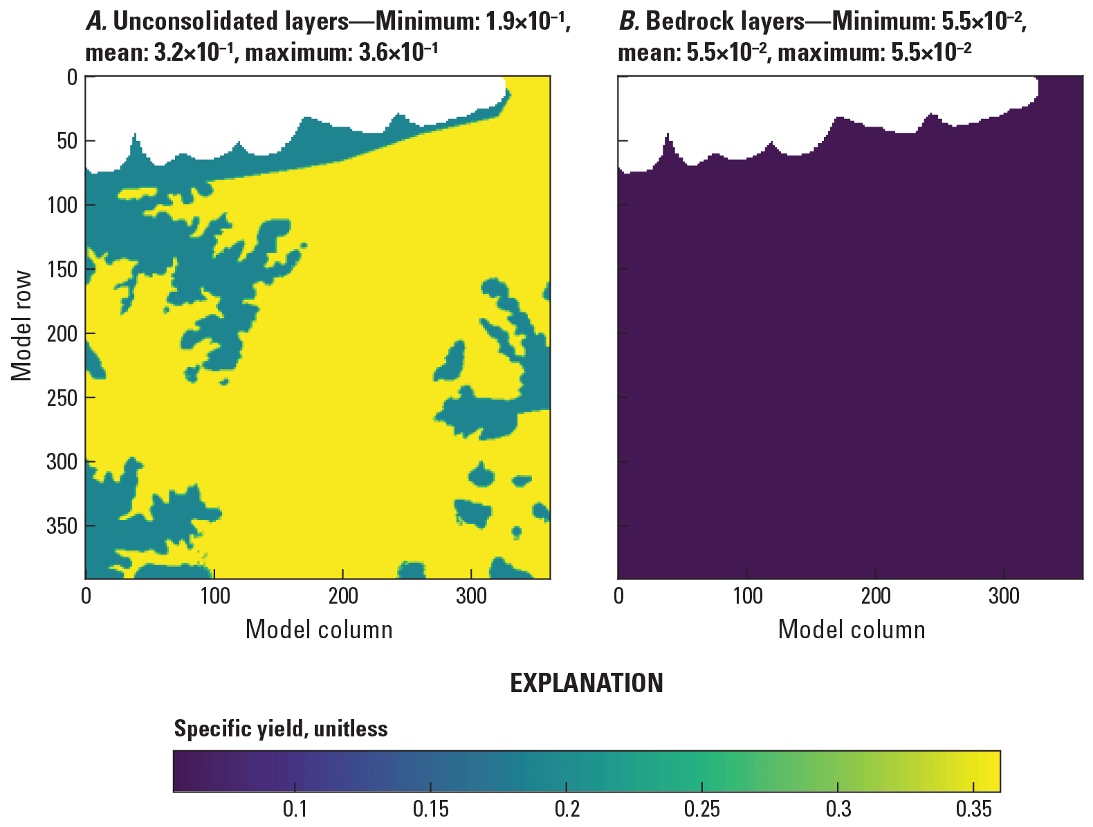
Specific yield for the unconsolidated and bedrock layers.

Specific storage for the unconsolidated and bedrock layers.
Table 6.
Summary table of calibrated specific yield values and literature ranges for the hydrostratigraphic units in the base model.[Except where other sources are cited, data are summarized from Reeves and Corson-Dosch (2023)]
| Hydrostratigraphic unit (app. 3) | Specific yield, unitless | |||||
|---|---|---|---|---|---|---|
| Mean | Median | Maximum | Minimum | Literature ranges from (Duffield, 2019) | Dane County model values (Parsen and others, 2016) | |
| Clay, silt-clay, mixed-fine, mixed-coarse, sand, sand-gravel, and gravel | 10.36 | 10.36 | 10.36 | 10.36 | 0.02–0.06 for clay; 0.20 for silt; 0.06–0.16 for till; 0.22–0.33 for sand; 0.19–0.28 for gravel | 0.015–0.3 for unconsolidated (calibrated model); 0.01–0.4 (calibration bounds). |
| Baraboo transition and weathered upper bedrock | 0.17 | 0.19 | 0.19 | 0.06 | See unconsolidated and bedrock values. | See unconsolidated and bedrock values. |
| Upper bedrock, Weathered Wonewoc, Wonewoc, Weathered Eau Claire, Eau Claire, and Mount Simon | 10.06 | 10.06 | 10.06 | 10.06 | 0.06–0.27 for sandstone; 0.12 for siltstone; 0.14–0.18 for limestone | None. |
Table 7.
Summary table of calibrated specific storage values and literature ranges for the hydrostratigraphic units in the base model.[Except where other sources are cited, data are summarized from Reeves and Corson-Dosch (2023)]
| Hydrostratigraphic unit (app. 3) | Specific storage, in 1 per foot | |||||
|---|---|---|---|---|---|---|
| Mean | Median | Maximum | Minimum | Literature ranges from (Duffield, 2019) | Dane County model values (Parsen and others, 2016) | |
| Clay, silt-clay, mixed-fine, mixed-coarse, sand, sand-gravel, and gravel | 18.3×10⁻⁶ | 18.3×10⁻⁶ | 18.3×10⁻⁶ | 18.3×10⁻⁶ | 1.5×10⁻⁵ to 6.3×10⁻³ | 7.1×10⁻⁵ to 5×10⁻³ for unconsolidated (calibrated model); 1×10⁻⁵ to 1×10⁻³ (calibration bounds) |
| Baraboo transition and weathered upper bedrock | 3.8×10⁻⁶ | 4.4×10⁻⁶ | 4.4×10⁻⁶ | 4.1×10⁻⁷ | See unconsolidated and bedrock values. | See unconsolidated and bedrock values. |
| Upper bedrock, Weathered Wonewoc, Wonewoc, Weathered Eau Claire, Eau Claire, and Mount Simon | 14.1×10⁻⁶ | 14.1×10⁻⁶ | 14.1×10⁻⁶ | 14.1×10⁻⁶ | 1×10⁻⁶ to 2.1×10⁻⁵ for fissured rock and <1×10⁻⁶ for sound rock (Duffield, 2019) | Not applicable for upper bedrock; 2.1×10⁻⁴ Wonewoc fracture layer (calibrated model) and 1×10⁻⁷ to 1×10⁻⁴ (calibration bounds) for Weathered Wonewoc; 2.6×10⁻⁵ (calibrated model); 1×10⁻⁷ to 1×10⁻³ for Wonewoc; 8.3×10⁻⁶ (calibrated model) and 1×10⁻⁷ to 1×10⁻³ (calibration bounds) for Weathered Eau Claire and Eau Claire; and 2.4×10⁻⁵ (calibrated model) and 1×10⁻⁷ to 1×10⁻³ for Mount Simon. |
Recharge
The PESTPP–iES calibration adjusted the initial potential recharge grids from the SWB model by no more than 15 percent. The calibrated multipliers on the potential recharge in the recharge calibration zones (see app. 2) ranged from 0.97 to 1.03, and the calibrated multipliers on the recharge from upland runoff watersheds ranged from 0.89 to 1.15. Table 8 shows the final calibrated average annual recharge and the minimum and maximum annual recharge for any of the years from 1980 through 2020 for the recharge calibration zones, and the same for the Baraboo Hills upland runoff values. The coarse-grained outwash had the highest average recharge, at almost 15 inches per year (in/yr), and the fine-grained sediments had the lowest amount, about 6 in/yr. The runoff from the upland watersheds averaged about 3.5–4 in/yr (over the watershed area). Over the full model simulation period (1980 through 2020), the average recharge across all zones was about 11.3 in/yr, average minimum recharge was about 5.3 in/yr, and average maximum recharge was about 19 in/yr.
Table 8.
Calibrated values for recharge in the base model, including average annual, minimum, and maximum for the years 1980 to 2020.[Data are summarized from Nielsen (2023)]
| Zone description | Calibration zone (app. 2) | Annual calibrated recharge for MODFLOW model, 1980 through 2020, in inches | Calibrated multiplier on potential recharge input | ||
|---|---|---|---|---|---|
| Average | Minimum | Maximum | |||
| Recharge zones (fig. 2.8) | |||||
| Baraboo Formation | rch_1 | 13.91 | 6.94 | 21.61 | 0.9705 |
| Big Flats Formation, finer grained | rch_2 | 10 | 4.98 | 17.01 | 0.9920 |
| Fine grained other | rch_3 | 6.01 | 2.84 | 9.87 | 1.0080 |
| Floodwater wash | rch_4 | 14.36 | 7.23 | 24.12 | 1.0082 |
| Hillslope fans | rch_5 | 11.15 | 5.4 | 18.58 | 1.0120 |
| Holocene stream sediments | rch_6 | 7.78 | 2.92 | 13.78 | 0.9984 |
| Mixed meltwater deposits | rch_7 | 12.3 | 5.68 | 20.65 | 0.9830 |
| Outwash | rch_8 | 14.97 | 7.37 | 25.22 | 1.0114 |
| Paleozoic sedimentary rocks | rch_9 | 9.56 | 5.04 | 15.17 | 0.9984 |
| Thin till over bedrock | rch_10 | 12.39 | 5.24 | 20.81 | 0.9907 |
| Till over outwash | rch_11 | 12.44 | 5.01 | 22.09 | 1.0290 |
| Runoff zones (fig. 2.6) | |||||
| Otter Creek watershed | runoff_10 | 3.49 | 0.97 | 11.87 | 0.8903 |
| Small watershed west | runoff_11 | 3.65 | 1.15 | 11.85 | 0.8907 |
| Small watershed middle | runoff_12 | 3.49 | 1.03 | 12.21 | 0.9010 |
| Small watershed east | runoff_13 | 4.15 | 1.19 | 15.21 | 1.1495 |
Drain and River Conductance
The calibrated conductance values for the river ranged from 634 to 17,428 square feet per day (ft2/d) above the dam with the lowest values in the zone closest to the dam and increasing upstream from the dam. Downstream from the dam, the conductance was 42,401 ft2/d in the tailwater zone and 30,785 ft2/d in the lower reach. Assuming a riverbed sediment thickness of 1 ft and using the model cell size of 150 by 150 ft, these river conductance values correspond to a hydraulic conductivity of the stream sediment between 0.03 and 1.9 feet per day (ft/d). Numerical experimentation showed that the pattern of river conductance was important for the MODPATH particle paths. For the drain cells, the calibrated multiplier was 1.048 giving a conductance of 39,300 ft2/d that, using the same assumptions as the river conductance, is an equivalent hydraulic conductivity of the wetland sediment of 1.75 ft/d.
Targets
Appendix 4 provides a full discussion of all the calibration target sets and presents the calibration results for each observation set. In general, calibration residuals for the synoptic hydraulic head observation sets had low misfit (mean absolute error) and minimal bias (mean error); thus, observed and simulated values fell near the 1:1 line on the plots in appendix 4. The model was best able to reproduce the synoptic hydraulic heads (set 1), the hydraulic head difference with the Wisconsin River (set 2), the mini-piezometers (set 3), and synoptic hydraulic heads in the plume areas (set 13). The model achieved the general trend but missed the magnitude slightly with the MIRM (set 6) and water table rise (set 5). The model had poorer performance with the lateral gradients in set 7 (although these are zero-weighted, so they do not affect the parameter adjustment) but slightly better performance with the wider-spaced gradients in set 14. The model did not match the Otter Creek flows well. Because Otter Creek is not in the immediate area of interest, this misfit was deemed acceptable for the purposes of simulating groundwater flows near the plumes.
A map (fig. 23) of the hydraulic head residuals for the set 1 (synoptic hydraulic heads) observation data were plotted across the model domain to assess if spatial bias exists in the base model groundwater elevations. High and low hydraulic head residuals for the set 1 synoptic calibration targets were generally distributed across the domain but showed some spatial bias with overestimated heads in the northwestern part of the former BAAP site. Residuals were smallest near the DBG plume and at the southern end of the PBG plume.
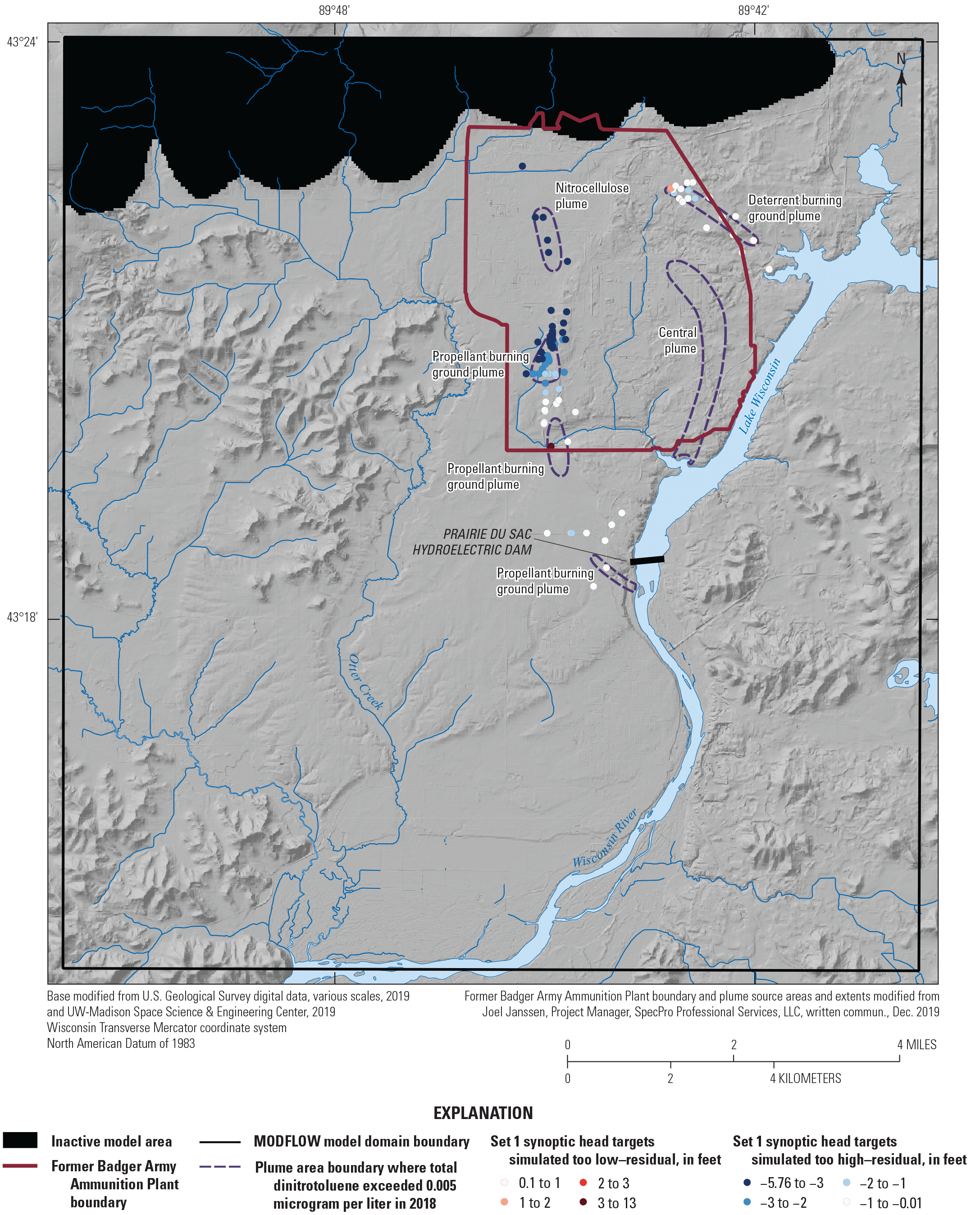
Spatial distribution of hydraulic head target residuals from set 1 synoptic, water year 2020.
Timeseries hydrographs for the observation set 3 and 4 wells that had extended records are shown in appendix 4, along with a map of well locations. In general, the simulated hydrographs showed patterns similar to the observed records but did not always match the magnitude of change. The timing of the trend was often slightly earlier in the simulated results, potentially because of a model structural error of not modeling the unsaturated zone and, therefore, the potential lag from when recharge infiltrates out of the root zone to when it hits the water table.
The three primary plumes at the site also provide information about the groundwater flow field. Plumes are estimates of contaminant distributions at the site based on observed values collected at monitoring wells. The plume shapes used in the calibration trials are simple polygons based on the plumes provided by Joel Janssen, Project Manager, SpecPro Professional Services, LLC (written commun., December 19, 2019). The particle-tracking model MODPATH (Pollock, 2016) was used to release simulated particles at areas designated as source zones at the site and forward track the movement of those particles with the flowing groundwater. The observations specified for the PESTPP–iES were the summed distances of every particle from the plume corresponding to the particle starting location over the whole simulation time (see app. 4). If a particle was within the plume shape, zero was assigned. The target observation specified for PESTPP–iES was zero for each plume; therefore, these observations are penalties on simulations that spread particles well outside the estimated plume shapes. In preliminary testing, particles for the DBG and PBG plumes were usually discharged to the river near the end of the simplified plume shapes. For the central plume, however, particles often stayed in the groundwater system and travelled towards the dam far past the simplified plume shape. Because the particles are only showing the potential flow paths and these targets are being used to help calibrate the groundwater-flow, particles from the central plume that travel beyond the end of the interpolated plume are not considered. For all the plumes, the particles are being used to indicate the flow field and are not meant to imply that contamination above site enforcement concentrations extends that far. The pre-calibration values for parameters and estimated ranges, an ensemble of 300 parameter sets, produced particle tracks that spread across the site and did not follow the plume shapes well (fig. 24A). After calibration iteration 3, the particle tracks from the remaining 202 realizations are more constrained to the plume shapes (fig. 24B). For particles tracking flow in the PBG plume area, many of the realizations in the ensemble of 202 runs had a few particles reaching the bedrock. Conversely, very few realizations had any particles reaching the bedrock in the central or DBG plume areas. The particles reaching bedrock results are consistent with observations from the site that only low concentrations, below action limits, have been reported in some bedrock observation wells. The potential for contaminants to reach the bedrock has important implications for remediation because contamination in the bedrock may move slowly and be more difficult to remove. These refined groundwater flow fields should be useful in estimating the advective component of the transport of contaminant. Note, that the particle tracking does not suggest contaminant concentration because particles do not have a starting concentration and other transport processes like contaminant dispersion, sorption to aquifer material, chemical reactions, or degradation are not included.
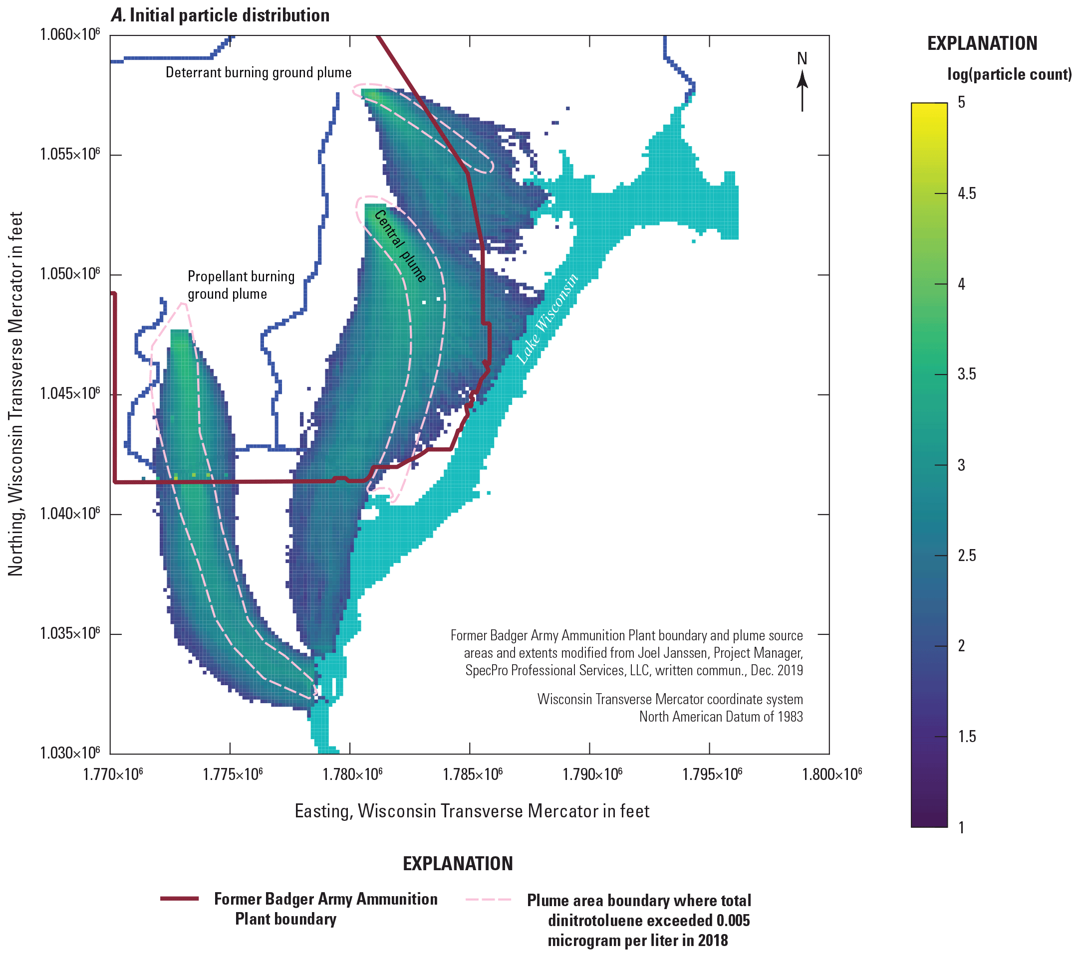
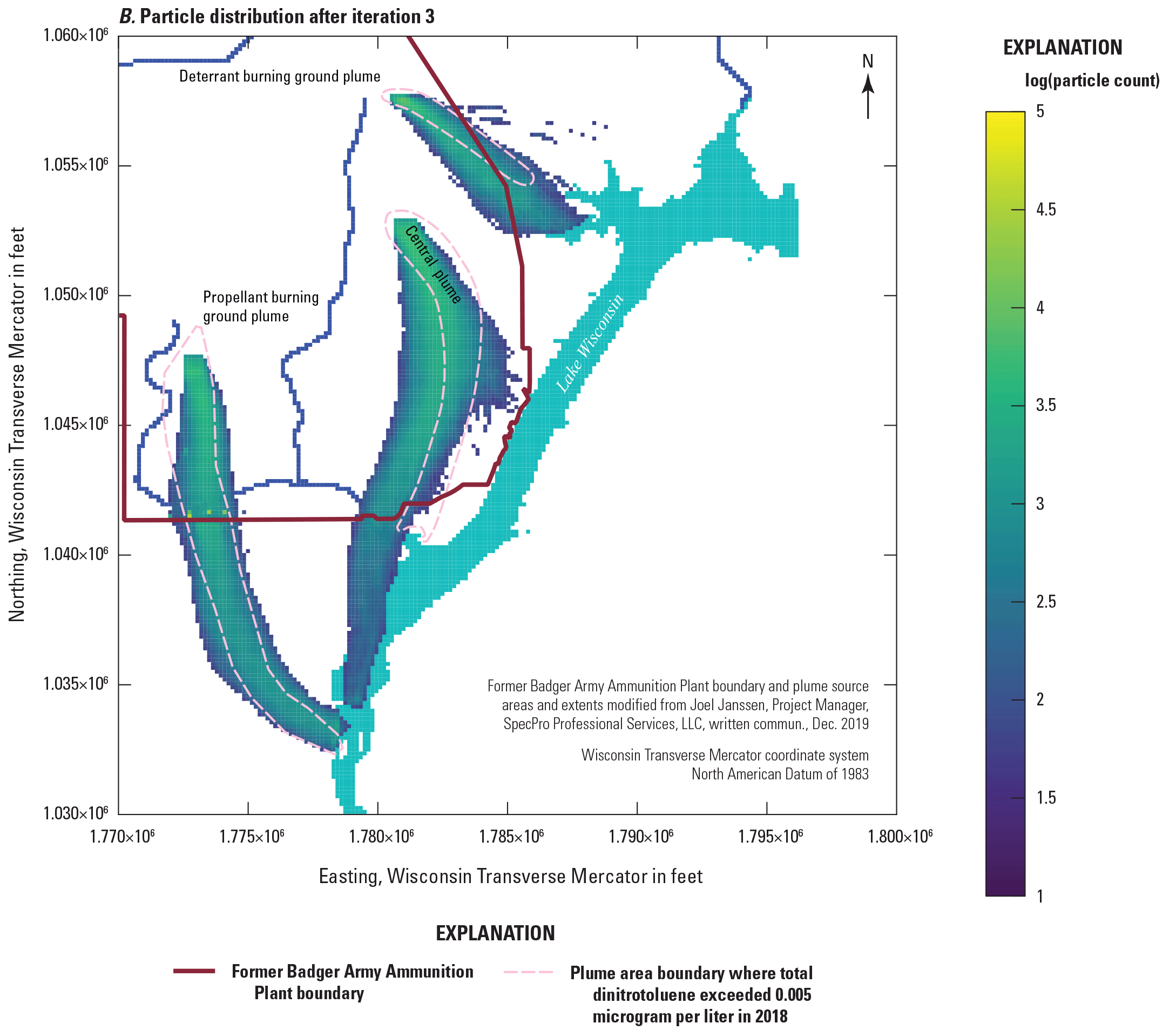
Starting and final particle path ensembles from MODPATH tracking of particles released in the plume source areas.
Groundwater Flow Model Results and Discussion
Groundwater inflows to and outflows from the model area (groundwater budget) are shown in figure 25. Sources of groundwater inflow included recharge (RECHARGE_IN), regional groundwater coming through the model boundary (WELLS_IN), losing streams (STREAM_LEAKAGE_IN), and where the Wisconsin River loses water to the aquifer (RIVER_LEAKAGE_IN). Major outflows from the groundwater system were groundwater seepage to wetlands via drains (DRAINS_OUT), discharge to streams (STREAM_LEAKAGE_OUT), and the Wisconsin River (RIVER_LEAKAGE_OUT); groundwater pumping (MNW2_OUT); and water leaving through the model boundaries (WELLS_OUT). The rest of the water balance is through water entering or leaving the aquifer storage through changes in the groundwater level or hydraulic head. Storage terms are labeled consistently with MODFLOW terms where STORAGE_OUT is water entering storage and STORAGE_IN is water leaving storage. The simple statement of mass balance is that the change in storage in the model area must be equal to the difference between groundwater entering and leaving the model area.
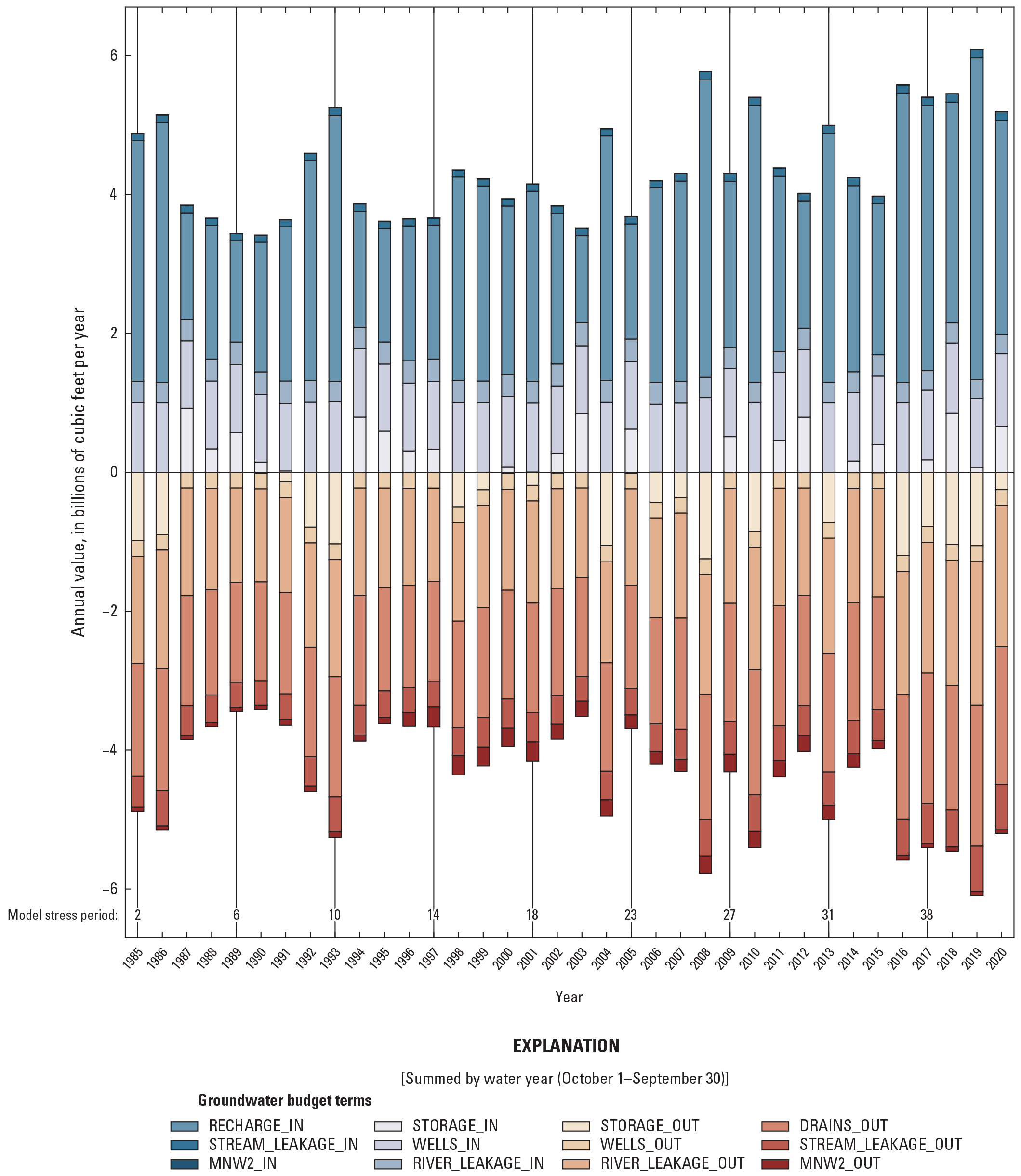
Annual groundwater budget summed by water year for each year in the model simulation period.
The modeled water table at the end of the simulation (September 2020) across the former BAAP is shown in figure 26. Groundwater flows from areas with high hydraulic heads to lower hydraulic heads perpendicular to the equal-elevation contour lines. Groundwater flow in the former BAAP is generally from the Baraboo Hills southeast to the Wisconsin River. The groundwater flow reflects a system in which water moves from topographic highs and other recharge areas to the Wisconsin River, streams, and low-lying wetland areas. Note the effect of the Prairie du Sac dam on the water table contours discussed below.
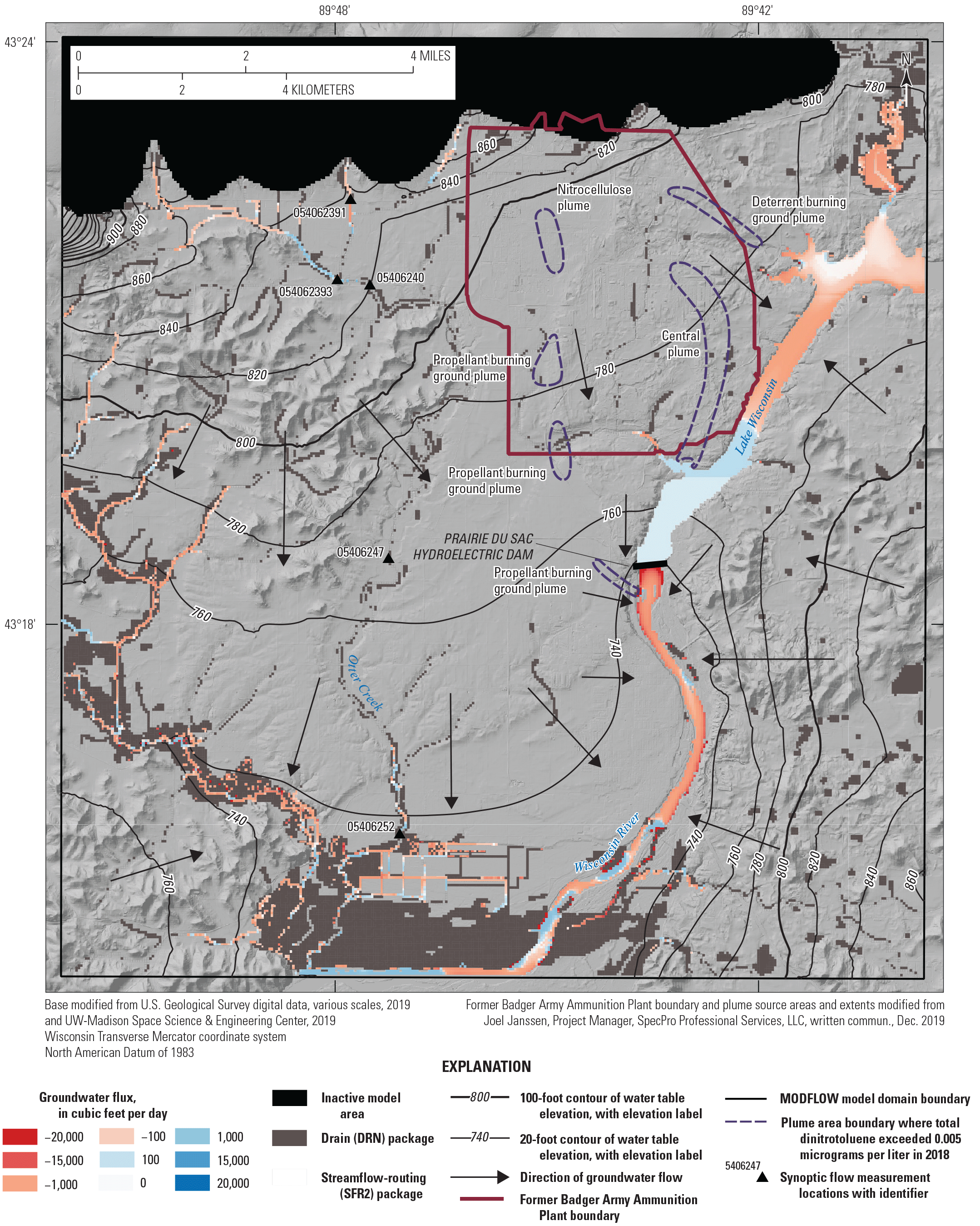
Simulated water table elevation from the base model and the groundwater fluxes to the Wisconsin River, streams, and drain cells. Both the contours and the fluxes represent conditions at the end of the final stress period (end of September 2020).
Streams, represented by SFR2 cells, and the Wisconsin River, represented by RIV cells, (fig. 13), can either be gaining water from the groundwater system or losing water to the groundwater system. As is expected in a humid temperate climate without appreciable pumping, the Wisconsin River is largely a regional groundwater sink, except for the area upstream from the Prairie du Sac hydroelectric dam where impounded water causes flow of river water into the aquifer. Just downstream from the dam, groundwater fluxes into the river are larger than other sections because of a steepened hydraulic gradient around the dam as the river elevation drops rapidly across the dam. Otter Creek is modeled as gaining in the headwaters, and then quickly becomes a losing stream and is largely dry by USGS site 05406240, until the stream section just upstream from site 05406252. The streamflow data (fig. 7) also show overall gaining conditions until site 05406240, then almost net neutral conditions to 5406247, and then net losing conditions down to site 05406252 (sites in fig. 6). The model overestimates dry conditions between sites 05406240 and 05406247. With streamflow generally less than 5 cubic feet per second, the larger dry section of stream is a relatively minimal amount of water. Because Otter Creek is not a focal point of this modeling effort, the modeled streamflows were considered acceptable. This streamflow misfit may slightly affect the location of the groundwater divide between water flowing either west to Otter Creek or east the Wisconsin River, but this error likely does not affect the movement of the plumes farther east.
Horizontal groundwater velocity is an estimate of how fast groundwater is moving laterally in the subsurface and contributes to the advective component of the contaminant transport. Horizontal groundwater velocity can be estimated by multiplying the horizontal hydraulic conductivity by the horizontal hydraulic gradient and dividing by the effective porosity. Alternatively, MODPATH particle track results can provide a more detailed estimate of the velocities. For each plume, particle velocities were calculated by dividing the distance every particle traveled by the corresponding travel time. The velocity results for the three plumes are plotted for each realization in figure 27. The mean horizontal velocity across all realizations is 1.69 ft/d for the PBG, 0.53 ft/d for the DBG, and 0.81 ft/d for the central plumes. Using well data from 2017 and 2018 and an effective porosity of 0.26, SpecPro Professional Services, LLC (2019) estimated groundwater velocities of 0.84 ft/d for the PBG, 0.30 ft/d for the DBG, and 0.39 ft/d for the central plumes. Zeiler (2002) estimated a groundwater velocity between 0.48 and 1.47 ft/d for the PBG plume. From this comparison with other sites estimates, the mean MODPATH particle velocities are similar but higher than those reported in other studies. The MODPATH simulations all used an effective porosity of 0.26. The range of the particle velocities simulated by the model has important implications on contaminant transport. To better constrain the flow model, a travel-time observation would be necessary.
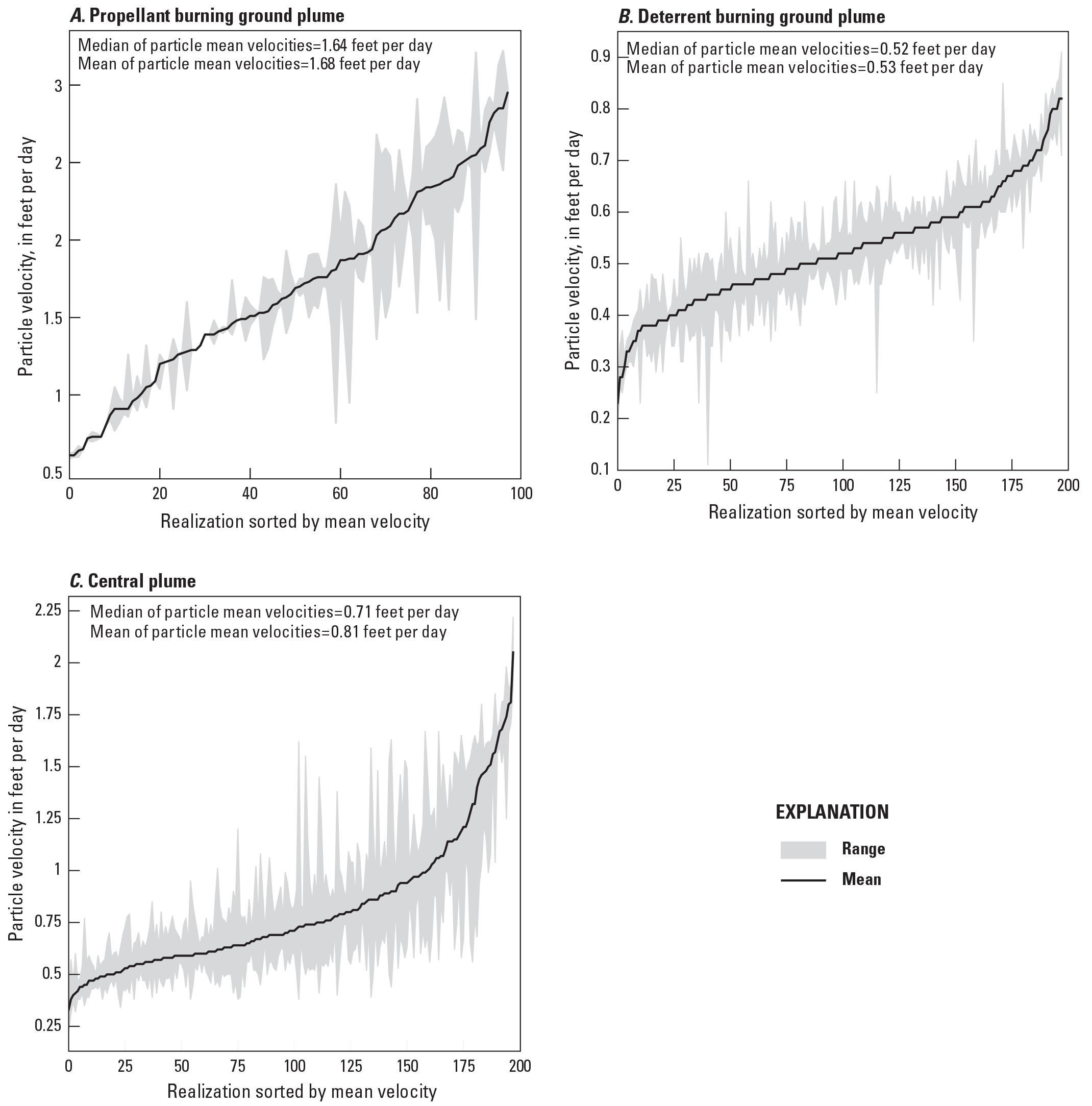
Horizontal groundwater velocities for each model realization, ordered by increasing mean velocity.
Assumptions and Limitations
The construction and subsequent utility of any model depends on the purpose of the model. The Badger model described here focused on simulations of groundwater flow across the former BAAP, particularly near the PBG, DBG, and central plumes. This purpose limits the model utility to site-scale evaluations, understanding general groundwater flow patterns, and exploring groundwater/surface-water interaction patterns across the former BAAP site during the transient period simulated. Focusing on other areas, such as a detailed examination of Otter Creek, would require updates to the model and potentially re-calibration. To convert a complex natural system into a numerical model, assumptions were made using available data and application of hydrologic principles based on modeling experience where data on the system were unavailable. Some key assumptions are described in this section.
The Badger model, like all models, is a simplified representation of a natural system of unknowable complexity. Although an effort was made to include all available information in the model, information on the groundwater system properties (for example, heterogeneity in the hydraulic conductivity field) or the system state (transient water levels and flows) is minimal across much of the model domain. Therefore, the model is not only simplified but also conditioned on an incomplete set of data. These two factors contribute to “structural error” in the model (Doherty and Welter, 2010), which can cause inaccuracies in areas where the model predictions are particularly sensitive to the uncertain input parameters. An effort was made to limit the effects of structural error to localized areas by distributing the parameterization of aquifer properties like hydraulic conductivity across the model grid using pilot points. One possible structural error is the presence of undetected heterogeneity (for example, preferential flow seams in the form of gravel lenses) that could lead to underestimates of plume transport even though overall rates of flow are properly simulated.
Scarce information on the unconsolidated material just above the bedrock and on the bedrock itself required simplifying assumptions about these units. These simplifying assumptions about the geology could interfere with the model’s ability to properly simulate downward flow from the lower part of the glacial aquifer to the bedrock. Local information about the bedrock properties is also scarce, although the existing information suggests that the Eau Claire does act as a confining unit between the Wonewoc and Mount Simon. These limitations could have important implications for transport and predicted remedial outcomes for contaminants in the bedrock versus the glacial aquifer.
Surface infiltration of precipitation was the dominant source of water to the groundwater system in the model area. A key assumption was that the pattern of net infiltration calculated by SWB was representative of actual groundwater recharge after calibration multipliers were applied to account for overall bias in the SWB results. One limitation of the recharge calibration was a lack of flux data, such as streamflow on the site, which make it difficult to isolate a unique recharge solution given the correlation among model parameter sets. SWB is an excellent tool for estimating transient recharge to the water table, but it is predicated on many assumptions that may lead to bias in the magnitude and timing of estimates. For example, the SWB model produces estimates of infiltration past the rooting zone, and no adjustment is made for the time it takes for water to percolate through the unsaturated zone to the water table; this lack of adjustment possibly is responsible for the lags noted in the water level timeseries datasets from site wells with longer historical records. For most of the simulation, the model stress periods were 1 year in duration, extending across the water year from the beginning of October to the end of September. The integrated SWB estimate over each year, although properly calculated from a water budget standpoint, may not fully represent recent recharge conditions at the end of the time step, which have greater effect on the head calibration targets (which usually corresponded to September measurements). For these reasons, using the model to assess water table behavior at a seasonal or monthly scale will be potentially complicated by this lag.
In addition to infiltration of precipitation, recharge derived from runoff from the Baraboo Hills could be important in controlling water levels near the base of the Baraboo Hills and base flow in Otter Creek. Available data were used to constrain the amount of runoff, but the estimate of this flux is highly uncertain.
It was assumed that the calibrated, steady-state Columbia County model simulates flow realistically enough in the former BAAP site to extract reasonable perimeter boundary conditions. Furthermore, it was assumed that perimeter boundary conditions were set sufficiently distant that steady state boundaries would not appreciably affect the groundwater flow field in the plume areas of interest.
The available hydraulic head and streamflow data were not uniform in spatial coverage, quantity, and quality. Hydraulic head observations were concentrated within the former BAAP and often limited to small areas near the plumes. Much of the model domain had little hydraulic head data coverage. Of the available hydraulic head data, a lack of vertical gradient information, such as data from piezometers, limited the ability to represent flow between the unconsolidated aquifer and bedrock aquifer, and the shallow and deep bedrock aquifers. Furthermore, streamflow data in Otter Creek only included recent data collected as part of this study.
The use of particle tracking to show the movement of groundwater at the site near the plumes was done to produce simulations that captured the observed advective transport of contaminants at the site. The hypothetical particles are not affected by dispersion, sorption of particles to aquifer material, reactions, or decay; and, therefore, are not meant to simulate contaminant transport or suggest where contaminant concentrations may exceed action limits. The particles also were released in 1984, which would most likely be well after contamination was released at the site. Part of the modeling study was done to constrain the flow field to produce reasonable advective particle movement based on the contaminant data collected at the site.
Because the model purpose drives decisions regarding appropriateness of assumptions used, simulation of future or different site conditions would require augmentation, refinement, and recalibration of the current model with the new model purpose in mind. The purpose of this calibration was to support future transport model efforts at the former BAAP site.
Summary
The former Badger Army Ammunition Plant (BAAP) produced smokeless gunpower and solid rocket propellent as munitions components with peak production periods during World War II, the Korean War, and the Vietnam War. Groundwater contamination investigations that began at the site in 1980 have found groundwater contamination plumes associated with the former munitions production. Various remediation actions have occurred since then, and monitoring is ongoing. An improved understanding of the groundwater flow system that is moving the contamination is needed to advance plans for future remediation efforts at the site and support discussion of groundwater issues associated with the former BAAP.
The groundwater flow system at the former BAAP was investigated using field data and a transient groundwater flow model built using the Newton Raphson formulation (MODFLOW–NWT) of the U.S. Geological Survey’s modular three-dimensional finite-difference. The model represented a transient period from 1984 to 2020. The model focused on the propellant burning ground, deterrent burning ground, and central plume areas where active remediation is being considered for dinitrotoluene contamination. Field data included synoptic measurements of Otter Creek streamflow, continuous measurement of groundwater levels in nested wells near the propellant and deterrent burning ground plume sources areas, synoptic mini-piezometer estimates of hydraulic gradient with the Wisconsin River, and slug testing in monitoring wells across the site. Field data were used to inform the structure and properties of the groundwater flow model and evaluate simulated groundwater levels and baseflow in Otter Creek. Particle tracking was performed using a MODPATH model with the MODFLOW–NWT solution to estimate groundwater flow through the contamination source area relative to mapped plume boundaries. The model key findings are as follows:
-
The overall groundwater flow direction across the former BAAP is generally from the Baraboo Hill and other topographic highs towards the Wisconsin River.
-
The Prairie du Sac hydroelectric dam locally affects the groundwater exchange with the Wisconsin River and has an important effect on the plume paths, particularly for the central plume.
-
Over the model simulation period (1980 through 2020), the average recharge across all recharge zones was about 11.3 inches per year; average minimum recharge was about 5.3 inches per year; and average maximum recharge was about 19 inches per year.
-
Based on the particle tracks for particles released near the source areas, the flow field in the plumes is well-simulated and should allow for a reasonable advective component in future transport modeling.
-
Using an ensemble approach for the flow model calibration leads to parameter distributions that represent uncertainty at the site, which may allow future designs to focus on risk, identify potential conditions that would impede remediation, and propose observations to test those conditions.
References Cited
Attig, J.W., and Clayton, L., 2003, Geology of Sauk County: Wisconsin Geological and Natural History Survey Information Circular 67–DI, digital data, accessed December 19, 2019, at https://wgnhs.wisc.edu/catalog/publication/000317/resource/ic67di.
Brown, B.A., Peters, R.M., and Massie-Ferch, K.M., 2013a, Preliminary bedrock geology of Dane County, Wisconsin [plate 1]: Wisconsin Geological and Natural History Survey WOFR2013–01–plate01, scale 1:100,000, accessed September 16, 2021, at https://wgnhs.wisc.edu/catalog/publication/000913/resource/wofr201301plate01.
Brown, B.A., Peters, R.M., and Massie-Ferch, K.M., 2013b, Preliminary geologic cross sections of Dane County, Wisconsin [plate 2]: Wisconsin Geological and Natural History Survey WOFR2013–01–plate02, scale 1:100,000, accessed September 16, 2021, at https://wgnhs.wisc.edu/catalog/publication/000913/resource/wofr201301plate02.
Carson, E.C., Rawling, J.E., III, Daniels, J.M., and Attig, J.W., 2019, v. 543. The physical geography and geology of the driftless area—The career and contributions of James C. Knox, Geological Society of America Special Paper, 156 p. [Also available at https://doi.org/10.1130/SPE543.]
Clayton, L., and Attig, J.W., 1990, Geology of Sauk County, Wisconsin: Wisconsin Geological and Natural History Survey Information Circular 67, 68 p., accessed September 16, 2021, at https://wgnhs.wisc.edu/catalog/publication/000317/resource/ic67.
Clayton, L., and Attig, J.W., 1997, Pleistocene geology of Dane County, Wisconsin (version 2) [GIS data]: Wisconsin Geological and Natural History Survey Bulletin 95–DI, accessed April 21, 2021, at https://wgnhs.wisc.edu/catalog/publication/000119.
Corson-Dosch, N.T., and Haserodt, M.J., 2023, Slug test analysis results from unconsolidated and bedrock aquifers at Badger Army Ammunition Plant, Sauk County, Wisconsin, 2020: U.S. Geological Survey data release, https://doi.org/10.5066/P95TSI73.
Cunningham, W.L., and Schalk, C.W., comps., 2011, GWPD 17—Conducting an instantaneous change in head (slug) test with a mechanical slug and submersible pressure transducer, chap. 17 of Cunningham, W.L., and Schalk, C.W., comps., Groundwater technical procedures of the U.S. Geological Survey: U.S. Geological Survey Techniques and Methods, book 1, chap. A1, 151 p., accessed March 2021 at https://pubs.usgs.gov/tm/1a1/.
Dalziel, I.W.D., and Dott, R.H., Jr., 1970, Geology of the Baraboo District, Wisconsin—A description and field guide incorporating structural analysis of the Precambrian rocks and sedimentologic studies of the Paleozoic strata: Wisconsin Geological and Natural History Survey Information Circular 14, 164 p., accessed September 16, 2021, at https://wgnhs.wisc.edu/catalog/publication/000264/resource/ic14.
Doherty, J., and Welter, D., 2010, A short exploration of structural noise: Water Resources Research, v. 46, no. 5, 14 p., accessed November 2021 at https://doi.org/10.1029/2009WR008377.
Duffield, G.M., 2007, AQTESOLV for Windows—Version 4.5 user’s guide: HydroSOLVE, Inc., 529 p. [Also available at https://hwbdocuments.env.nm.gov/Los%20Alamos%20National%20Labs/General/37764.pdf.]
Duffield, G.M., 2019, Representative values of hydraulic properties: HydroSOLVE, Inc., AQTESOLV web page, accessed March 25, 2022, at http://www.aqtesolv.com/aquifer-tests/aquifer_properties.htm.
Gotkowitz, M.B., Leaf, A.T., and Sellwood, S.M., 2021, Hydrogeology and simulation of groundwater flow in Columbia County, Wisconsin: Wisconsin Geological and Natural History Survey Bulletin B117, 51 p., accessed September 2022 at https://wgnhs.wisc.edu/catalog/publication/000985.
Gotkowitz, M.B., Zeiler, K.K., Dunning, C.P., Thomas, J.C., and Lin, Y., 2005, Hydrogeology and simulation of groundwater flow in Sauk County, Wisconsin: Wisconsin Geological and Natural History Survey Bulletin 102, 51 p., accessed September 2021 at https://wgnhs.wisc.edu/pubshare/B102.pdf.
Hooyer, T.S., Mode, W.N., Clayton, L., and Attig, J.W., 2015, Preliminary Quaternary geology of Columbia, Green Lake, and Marquette Counties, Wisconsin: Wisconsin Geological and Natural History Survey Open-File Report 2015–01–DI, digital data, accessed December 12, 2019, at https://wgnhs.wisc.edu/catalog/publication/000928/resource/wofr201501di.
Hunt, R.J., White, J.T., Duncan, L.L., Haugh, C.J., and Doherty, J., 2021, Evaluating lower computational burden approaches for calibration of large environmental models: Ground Water, v. 59, no. 6, p. 788–798. [Also available at https://doi.org/10.1111%2Fgwat.13106.]
Hyder, Z., Butler, J.J., Jr., McElwee, C.D., and Liu, W., 1994, Slug tests in partially penetrating wells: Water Resources Research, v. 30, no. 11, p. 2945–2957. [Also available at https://doi.org/10.1029/94WR01670.]
Krohelski, J.T., Bradbury, K.R., Hunt, R.J., and Swanson, S.K., 2000, Numerical simulation of groundwater flow in Dane County, Wisconsin: Wisconsin Geological and Natural History Survey Bulletin 98, 32 p., accessed September 1, 2021 at https://wgnhs.wisc.edu/pubshare/B098.pdf.
Leaf, A.T., 2018, SFRmaker: GitHub software web page, accessed November 27, 2018, at https://github.com/DOI-USGS/sfrmaker.
Lundqvist, J., Clayton, L., and Mickelson, D.M., 1993, Deposition of the late Wisconsin Johnstown moraine, south-central Wisconsin: Quaternary International, v. 18, p. 53–59, accessed April 21, 2021, at https://doi.org/10.1016/1040-6182(93)90053-I.
McKay, L., Bondelid, T., Dewald, T., Johnston, C., Moore, R., and Rea, A., 2012, NHDPlus version 2—User guide: U.S. Environmental Protection Agency, accessed February 4, 2019, at https://nhdplus.com/NHDPlus/NHDPlusV2_home.php.
Nielsen, M.G., 2023, Soil-Water-Balance (SWB) model archive used to simulate potential annual recharge for the former Badger Army Ammunition Plant study area, Prairie du Sac, Wisconsin, 1980 to 2020: U.S. Geological Survey data release, https://doi.org/10.5066/P9S2IDV0.
Niswonger, R.G., Panday, S., and Ibaraki, M., 2011, MODFLOW–NWT, a Newton formulation for MODFLOW–2005: U.S. Geological Survey Techniques and Methods, book 6, chap. A37, 44 p., accessed December 2020 at https://pubs.usgs.gov/tm/tm6a37/.
Ostrom, M.E., 1965, Cambro-Ordovician stratigraphy of southwest Wisconsin: University of Wisconsin Geological and Natural History Survey Information Circular 6, 57 p. [Also available at https://wgnhs.wisc.edu/catalog/publication/000256.]
Parsen, M.J., Bradbury, K.R., Hunt, R.J., and Feinstein, D.T., 2016, The 2016 groundwater flow model for Dane County, Wisconsin: Wisconsin Geological and Natural History Survey Bulletin 110, 56 p., accessed September 1, 2021 at https://wgnhs.wisc.edu/catalog/publication/000935/resource/b110.
Pollock, D.W., 2016, User guide for MODPATH version 7—A particle-tracking model for MODFLOW: U.S. Geological Survey Open-File Report 2016–1086, 35 p., accessed December, 2019 at https://doi.org/10.3133/ofr20161086.
Reeves, H.W., and Corson-Dosch, N.T., 2023, Groundwater model archive for the former Badger Army Ammunition Plant, Wisconsin: U.S. Geological Survey data release, https://doi.org/10.5066/P9LNRILT.
SpecPro Professional Services, LLC, 2019, Remedial investigation/feasibility study for site-wide groundwater at the former Badger Army Ammunition Plant, Baraboo, Wisconsin: SpecPro Professional Services, LLC, 717 p., accessed March 2020 at https://cswab.org/wp-content/uploads/2020/05/Badger-Army-Site-Wide-Groundwater-RIFS-Study-DRAFT-Nov-2019.pdf.
Springer, R.K., and Gelhar, L.W., 1991, Characterization of large-scale aquifer heterogeneity in glacial outwash by analysis of slug tests with oscillatory responses, Cape Cod, Massachusetts, in Mallard, G.E., and Aronson, D.A., eds., U.S. Geological Survey toxic substances hydrology program—Proceedings of the technical meeting, Monterey, California, March 11–15, 1991: U.S. Geological Survey Water-Resources Investigations Report 91–4034, p. 36–40. [Also available at https://doi.org/10.3133/wri914034.]
Turnipseed, D.P., and Sauer, V.B., 2010, Discharge measurements at gaging stations: U.S. Geological Survey Techniques and Methods, book 3, chap. A8, 87 p., accessed September 2022 at https://doi.org/10.3133/tm3A8.
U.S. Geological Survey [USGS], 2019, USGS NED 1/3 arc-second n44w090 1 x 1 degree IMG 2019: U.S. Geological Survey dataset, accessed October 28, 2019, at https://www.usgs.gov/programs/national-geospatial-program/national-map.
U.S. Geological Survey [USGS], 2021, USGS water data for the Nation: U.S. Geological Survey National Water Information System database, accessed September 2021 at https://doi.org/10.5066/F7P55KJN.
University of Wisconsin–Madison, 2019a, Columbia, in UW–Madison Space Science & Engineering Center file repository: University of Wisconsin-Madison, Space Science & Engineering Center dataset, accessed October 30, 2019, at https://bin.ssec.wisc.edu/pub/wisconsinview/lidar/. [Columbia County data directly accessible at https://bin.ssec.wisc.edu/pub/wisconsinview/lidar/Columbia/.]
University of Wisconsin–Madison, 2019b, Sauk, in UW–Madison Space Science & Engineering Center file repository: University of Wisconsin-Madison, Space Science & Engineering Center dataset, accessed October 30, 2019, at https://bin.ssec.wisc.edu/pub/wisconsinview/lidar/. [Sauk County data directly accessible at https://bin.ssec.wisc.edu/pub/wisconsinview/lidar/Sauk/.]
Watermark Numerical Computing, 2020, Groundwater data utilities, part B—Program descriptions: Watermark Numerical Computing, accessed April 28, 2021, at https://pesthomepage.org/groundwater-utilities.
Westenbroek, S.M., Engott, J.A., Kelson, V.A., and Hunt, R.J., 2018, SWB version 2.0—A soil-water-balance code for estimating net infiltration and other water-budget components: U.S. Geological Survey Techniques and Methods, book 6, chap. A59, 118 p., accessed January 1, 2019, at https://doi.org/10.3133/tm6A59.
White, J.T., 2018, A model-independent iterative ensemble smoother for efficient history- matching and uncertainty quantification in very high dimensions: Environmental Modelling & Software, v. 109, p. 191–201. [Also available at https://doi.org/10.1016/j.envsoft.2018.06.009.]
White, J.T., Hunt, R.J., Fienen, M.N., and Doherty, J.E., 2020, Approaches to highly parameterized inversion—PEST++ version 5, a software suite for parameter estimation, uncertainty analysis, management optimization and sensitivity analysis: U.S. Geological Survey Techniques and Methods, book 7, chap. C26, 52 p. [Also available at https://doi.org/10.3133/tm7C26.]
Wisconsin Department of Natural Resources, 2016, Former Badger Army Ammunition Plant (BAAP) [draft map B]: Wisconsin Department of Natural Resources, map WM–SPRA–MP–9493–B, accessed September 17, 2021, at https://dnr.wi.gov/files/PDF/pubs/lf/LF0091Map_B_2016.pdf.
Wisconsin Department of Natural Resources, 2021, The Groundwater Retrieval Network: Wisconsin Department of Natural Resources, Drinking Water and Groundwater Program website, accessed February 9, 2021, at https://dnr.wisconsin.gov/topic/Groundwater/GRN.html.
Appendix 1. Groundwater Elevation Data Processing
Reference Cited
U.S. Geological Survey, 2020, SK-10/06E/02-0003, in USGS water data for the Nation: U.S. Geological Survey National Water Information System database, accessed December 10, 2020, at https://doi.org/10.5066/F7P55KJN. [Site 432100089440001 groundwater data directly accessible at https://waterdata.usgs.gov/monitoring-location/432100089440001/#parameterCode=72019&startDT=1989-06-30&endDT=2020-06-30.]
Appendix 2. Soil-Water-Balance Model Setup Details
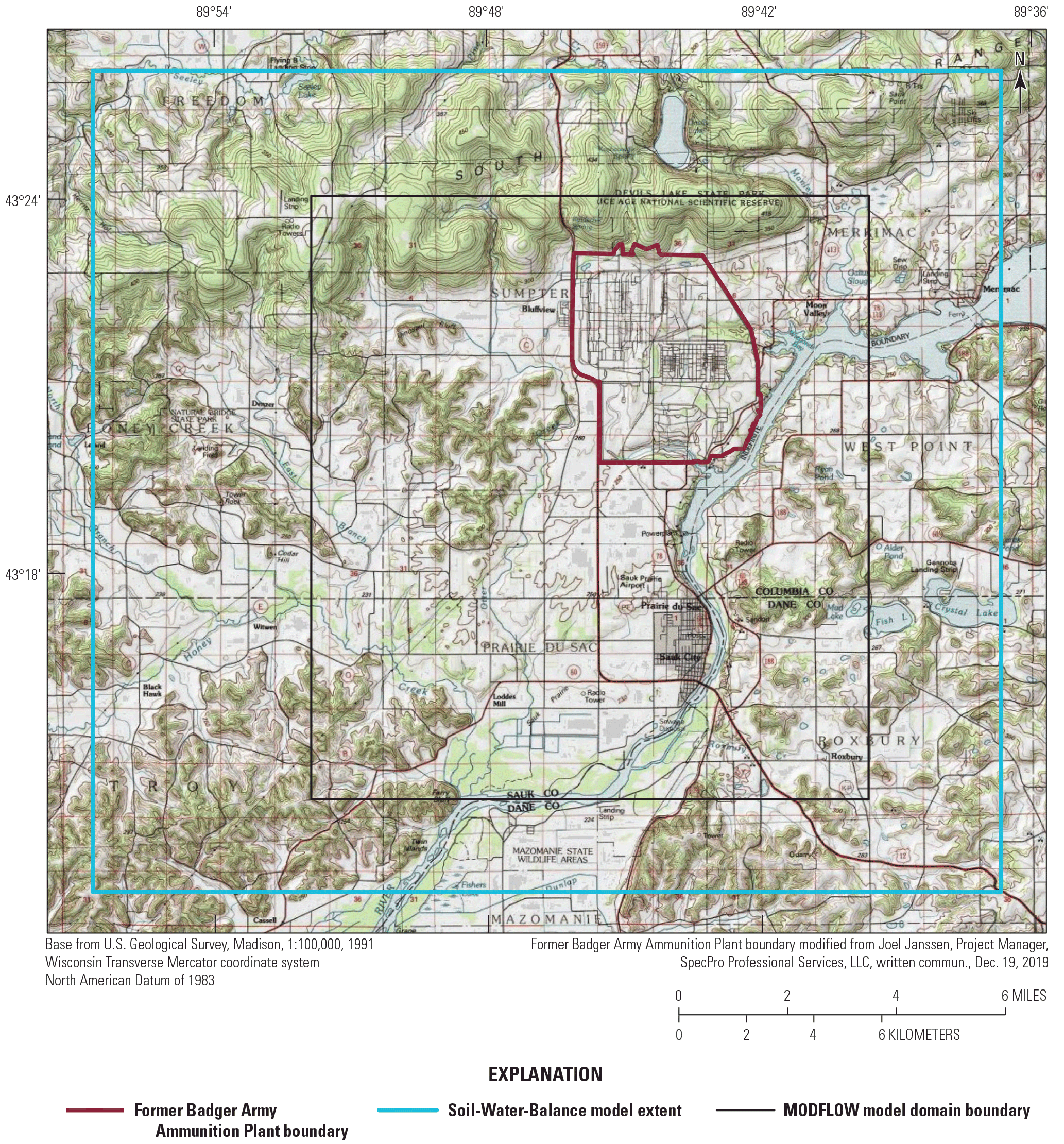
Soil-Water-Balance model extent for the former Badger Army Ammunition Plant study area.
Model Inputs
The U.S. Department of Agriculture (USDA) Natural Resources Conservation Service (NRCS) gridded national soil survey geographic database (gSSURGO) provided the base for the hydrologic soil groups (HSG) and the available water capacity (AWC) input data (Soil Survey Staff, 2018). The native dataset is rasterized at a 10-meter resolution that was then resampled to 30.48 meters for this study. The NRCS data for the top 150 centimeters were used for this study because many of the land uses have rooting zones that extend that deep and beyond. The hydrologic soil groups (U.S. Department of Agriculture, 2007) used in the study include the four basic HSGs (A, B, C, and D) and the dual HSGs (A/D, B/D, and C/D) modified to better represent the surficial geologic units in the study area (fig. 2.2). The AWC data for the top 150 cm (fig. 2.3) are expressed in units of inches per foot (in/ft) of soil thickness. The HSG and AWC data are gridded representations of mapped soil unit polygons, and the values assigned by lookup tables relate the soil unit properties to the soil unit polygon distribution.
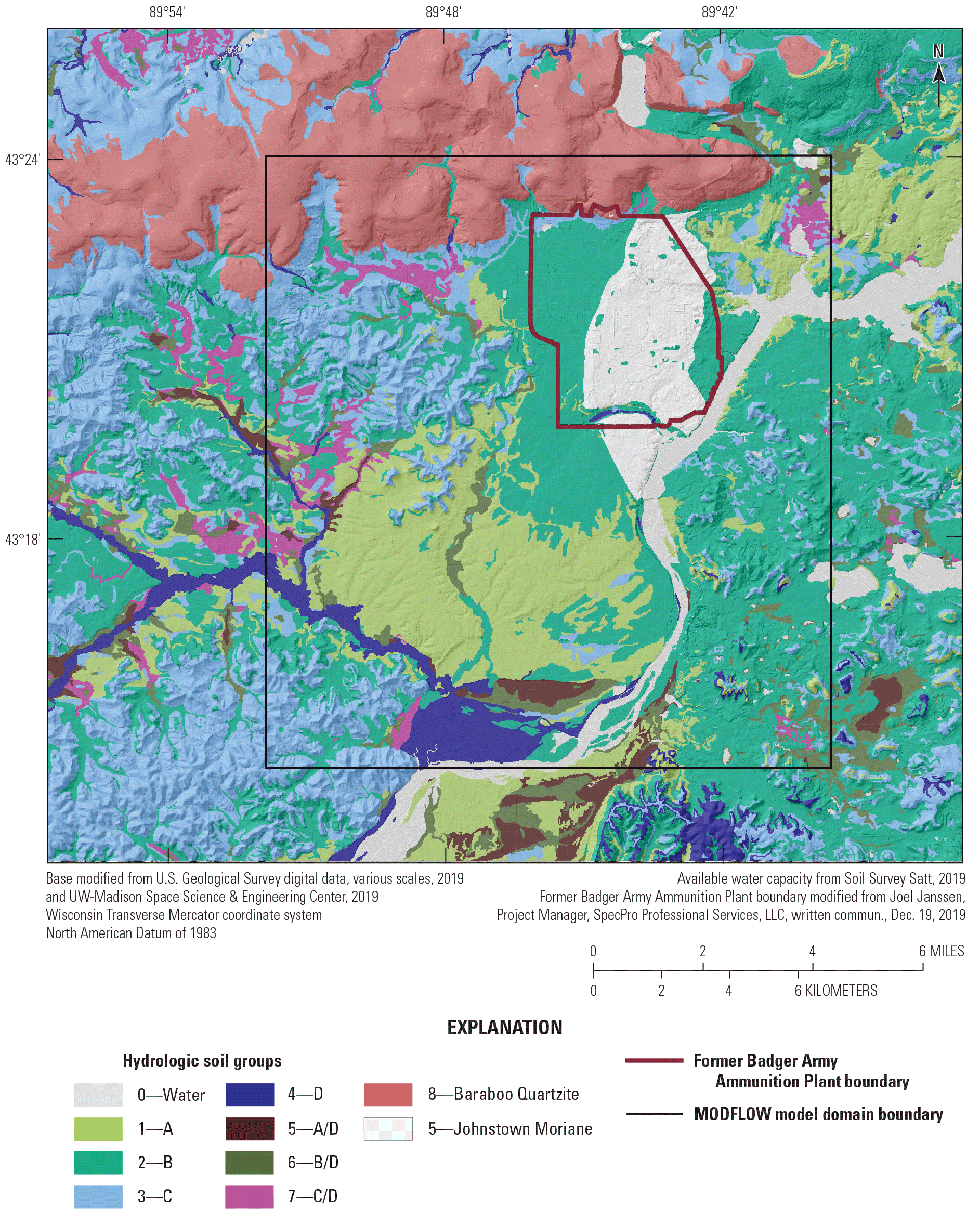
Mapped hydrologic soil groups for the former Badger Army Ammunition Plant Soil-Water-Balance model.
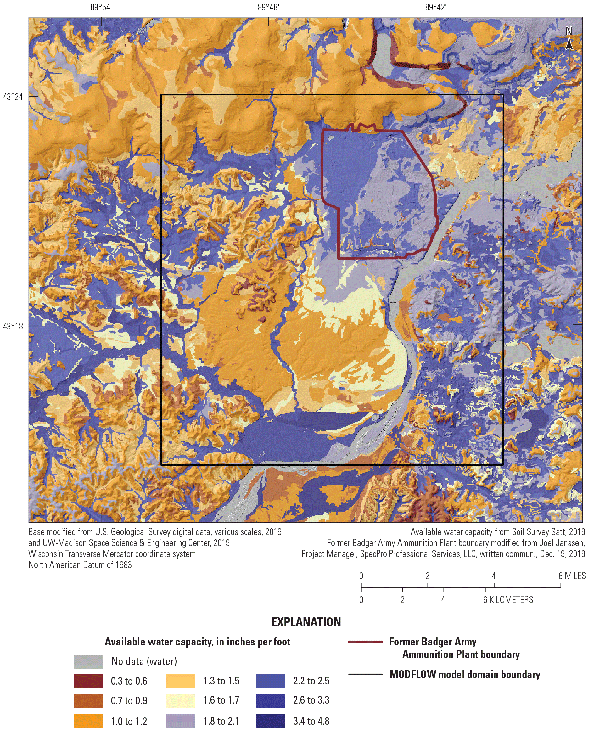
Mapped available water capacity grid for the former Badger Army Ammunition Plant Soil-Water-Balance model.
The SWB model input requirements include land use categories. The National Land Cover Dataset (Jin and others, 2019) was the primary source for land use data in the study area. During the time of the SWB simulation (1980–2020), the former BAAP was decommissioned: most of the structures were removed, and much of the land was converted to nonurbanized land uses. Therefore, the land use for SWB was input as annual grids, which were modified from the original source for the time after the removal of the buildings and restoration of the site began in the early 2000s. Although the National Land Cover Dataset includes versions for several years between 2008 and 2019, the data do not reflect the conditions on the ground in the former Badger Army Ammunition Plant area. No specific record of the removal and restoration was available for this study, so aerial photos available in Google Earth over the time of the removal and restoration were used to modify the available land use classification to conditions on the ground from 2005 through 2012, when the restoration was completed. The changes in land use for the study area are represented in the datasets for 2000 and 2020 (figs. 2.4, 2.5).
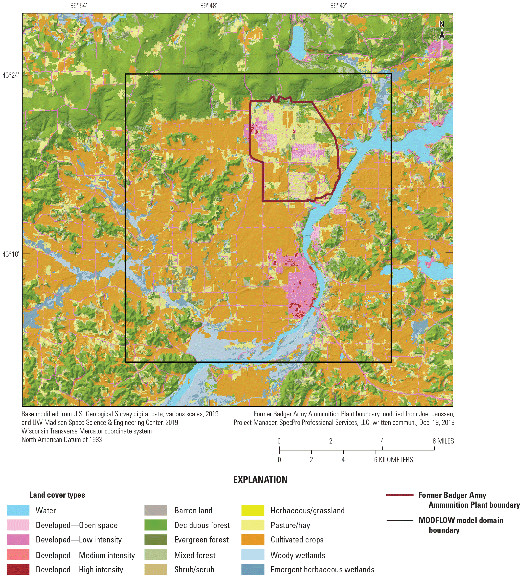
Land use for 2000 used in the Soil-Water-Balance model for the former Badger Army Ammunition Plant study area.
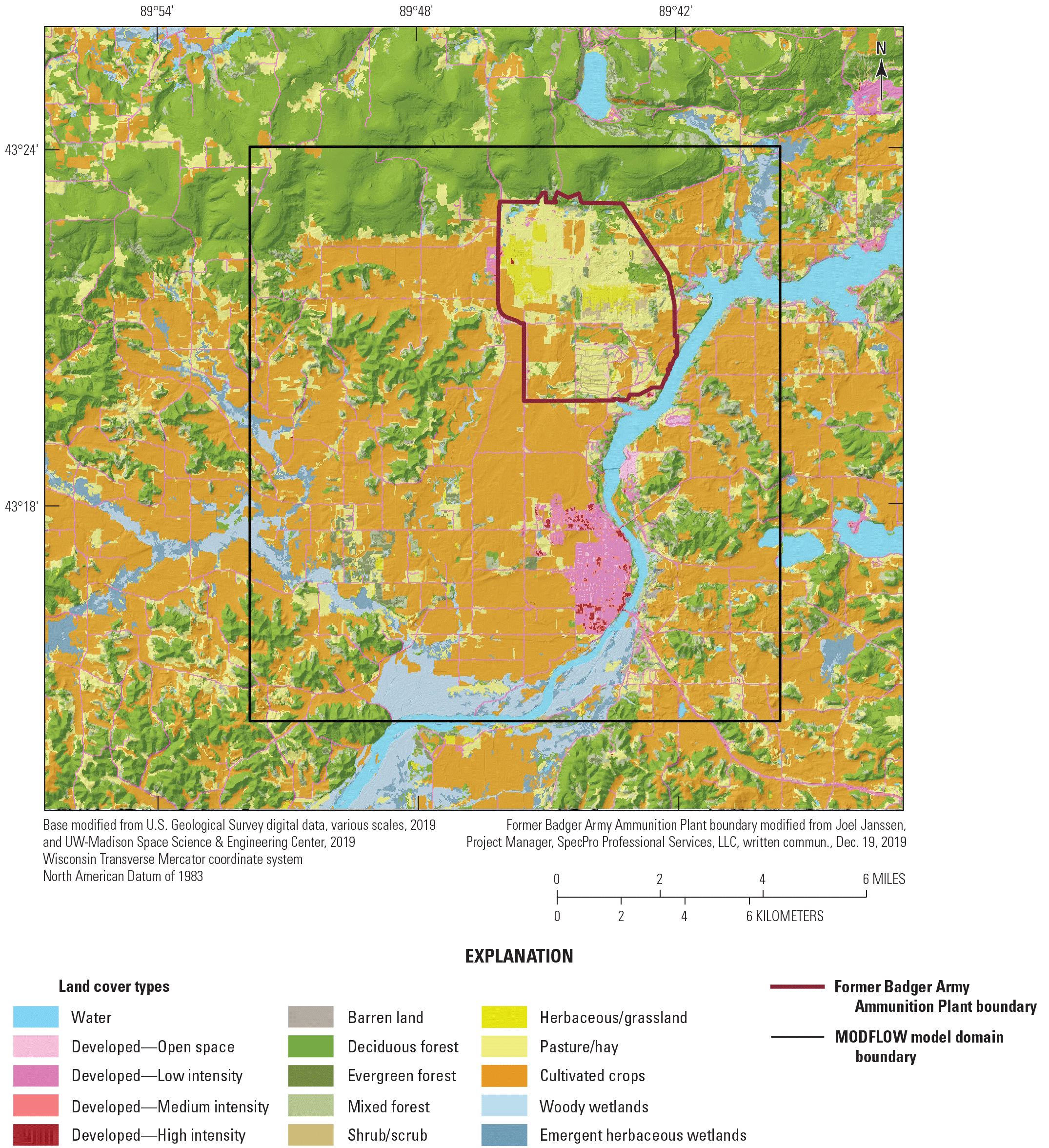
Land use for 2020 used in the Soil-Water-Balance model for the former Badger Army Ammunition Plant study area.
Daily climate data inputs are also needed for the SWB model. DayMet data (daily precipitation and minimum and maximum temperature) were used for the climate inputs (Thornton and others, 2016, 202052). To conserve computer storage, the grids were subset to an area about 2–3 miles beyond the Badger groundwater flow model area.
In addition to the spatial input datasets, the SWB model for the former BAAP study area used two lookup tables to calculate the water balance terms: a primary land-use lookup table, and a secondary irrigation lookup table, which was used to calculate the evapotranspiration part of the water balance using the FAO56 method (Allen and others, 1998; Westenbroek and others, 2018), which gives much greater control over the evapotranspiration simulation than the default Thornthwaite-Mather method (Thornthwaite and Mather, 1957) used by the SWB code. The primary land-use lookup table contains values for runoff curve numbers, maximum daily recharge, and rooting depths for each combination of land-use class and hydrologic soil group in the model (an example is shown in table 2.1; the full table is provided in the accompanying data release for the SWB model; Nielsen, 2023). With 15 land-use classes and 9 hydrologic soil groups, the SWB model potentially has 135 different values for each of these categories (although many combinations of land use and hydrologic soil group do not occur in the study area). Lookup values for interception (if used) vary with land use and growing season and are also included in the SWB land-use lookup table. The irrigation land-use table (an example in shown in table 2.2; the full table is provided in the accompanying data release for the SWB model; Nielsen, 2023) includes plant growth settings such as crop coefficients (Kcb values for onset of growth, plant maturity, and senescence), growing-season lengths, bare soil evaporation settings for every land-use class, and irrigation application settings for cultivated crops.
Table 2.1.
Example land-use lookup table used by the Soil-Water-Balance model.[These data are summarized from Nielsen (2023). A, B, B/D, and C/D are hydrologic soil groups used in the Soil-Water-Balance model]
The lookup table used in the Badger Army Ammunition Plant simulations has entries for all seven soil hydrologic groups and two extra surficial geologic units. This table only includes data for soil groups A, B, B/D, and C/D. See accompanying data release for the full table (Nielsen, 2023, LU_Lookup_Badger_v5.txt).
Table 2.2.
Example irrigation lookup table used by the Soil-Water-Balance model.[These data are summarized from Nielsen (2023). Dates are given in month/day. Kcb, transpiration crop coefficient; mid, middle; min, minimum; dev, standard deviation; A, B, B/D, and C/D are hydrologic soil groups used in the Soil-Water-Balance model]
The lookup table used in the Badger Army Ammunition Plant simulations has entries for all seven soil hydrologic groups and two surficial geologic units. This table only includes data for soil groups A, B, B/D, and C/D. See accompanying data release for the full table (Nielsen, 2023, IRR_Lookup_Badger_v4.txt).
Lookup table values for the SWB model were based on values from another USGS SWB model from central Wisconsin (Fienen and others, 2021) and calibrated to local soil conditions. A separate adjustment of the lookup tables for the former BAAP SWB model was done to ensure that the simulated runoff from the Baraboo Hills was within reasonable bounds. Otter Creek (fig. 1) is one of the watersheds with simulated runoff calculated by the SWB model and had eight discrete streamflow measurements made during the simulation period of this model. Data from these streamflow measurements were used to calculate daily runoff from the upstream watershed, and these were compared to the simulated values from the SWB model. The lookup table values were adjusted until a satisfactory visual match with the measured data was obtained.
Model Outputs
The SWB model produces daily gridded output for each of the water balance terms in network Common Data Form (.netCDF) format. The daily grids were processed using python scripts to produce the data needed for the groundwater flow model including Tag Image File Format (.tif) files of total potential recharge for each of the model time steps (see the “Stress Periods” section of this report) and upland runoff from each of four watersheds in the Baraboo Hills that spills onto the outwash plain (shown in fig. 2.6). An illustration of the variation in annual average potential recharge for the study area is shown in figure 2.7. Generally, potential recharge is highest in the coarse-grained soils on the outwash plains and much lower where the soils are clay rich. The year-to-year variability in annual recharge is quite large, illustrated by the years 2018 and 1990, where the potential recharge in 2018 is roughly double that in 1990.
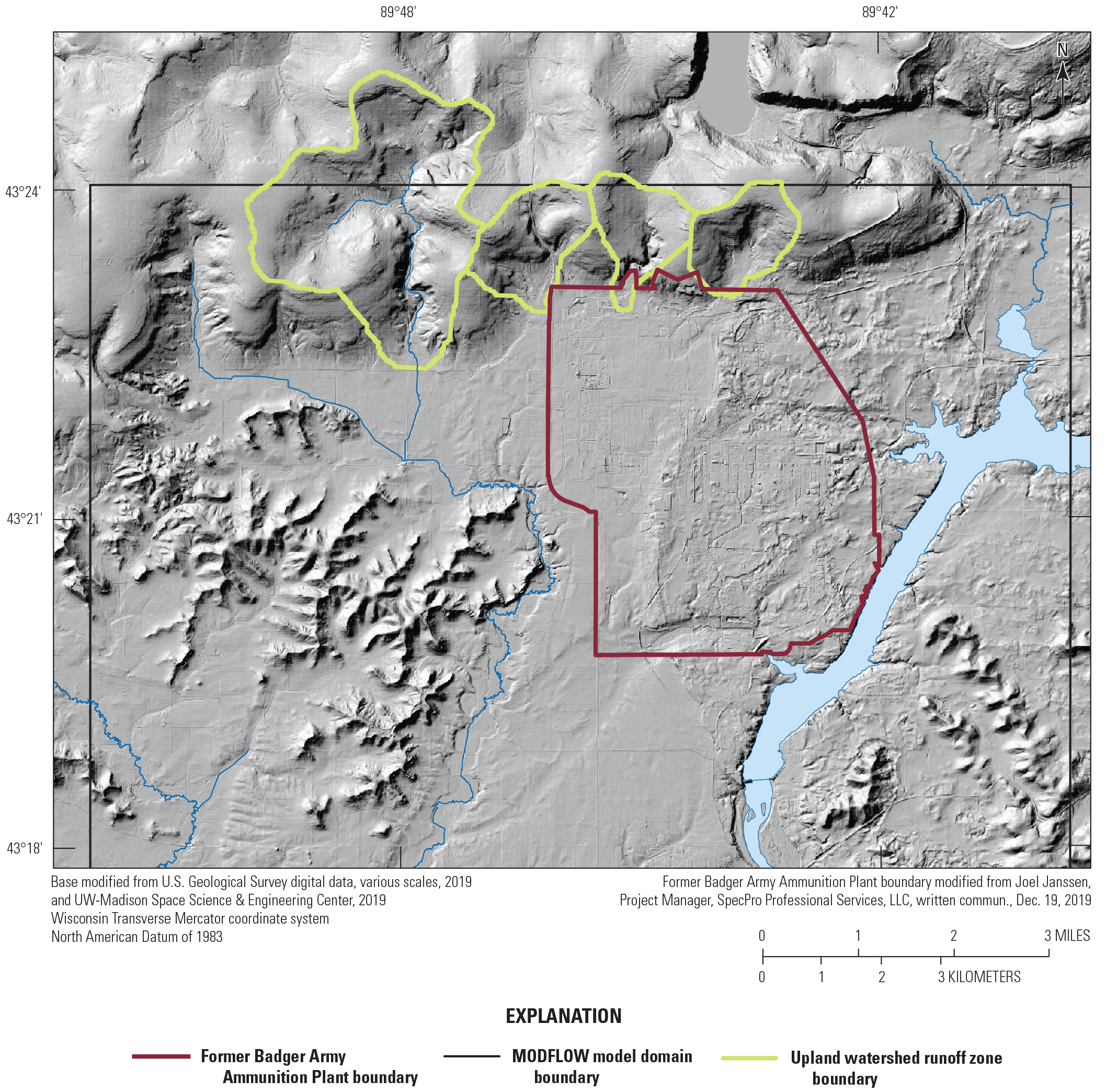
Upland watershed zones contributing runoff to the edge of the outwash and till plain of the former Badger Army Ammunition Plant study area.
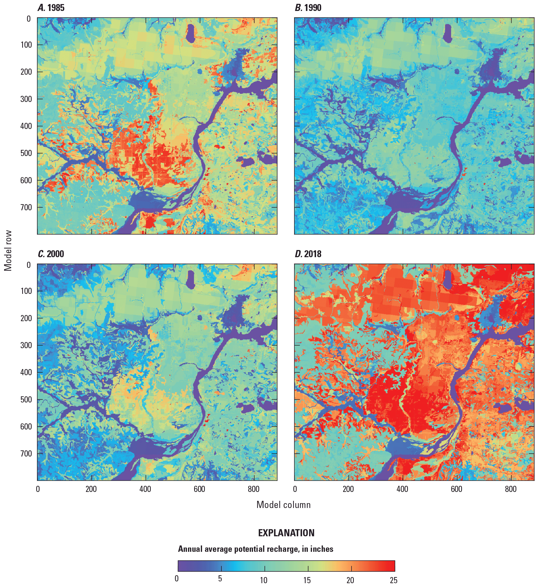
Annual average potential recharge for the Soil-Water-Balance model of the former Badger Army Ammunition Plant site.
The groundwater flow model calibration included slight adjustments of the SWB potential recharge, using 11 calibration zones. The zones used for calibration of the potential recharge were based primarily on the surficial geology related to the potential permeability of the surficial units and are listed in table 2.3 and depicted in figure 2.8.
Table 2.3.
Descriptions of the calibration recharge zones used in the groundwater flow model calibration.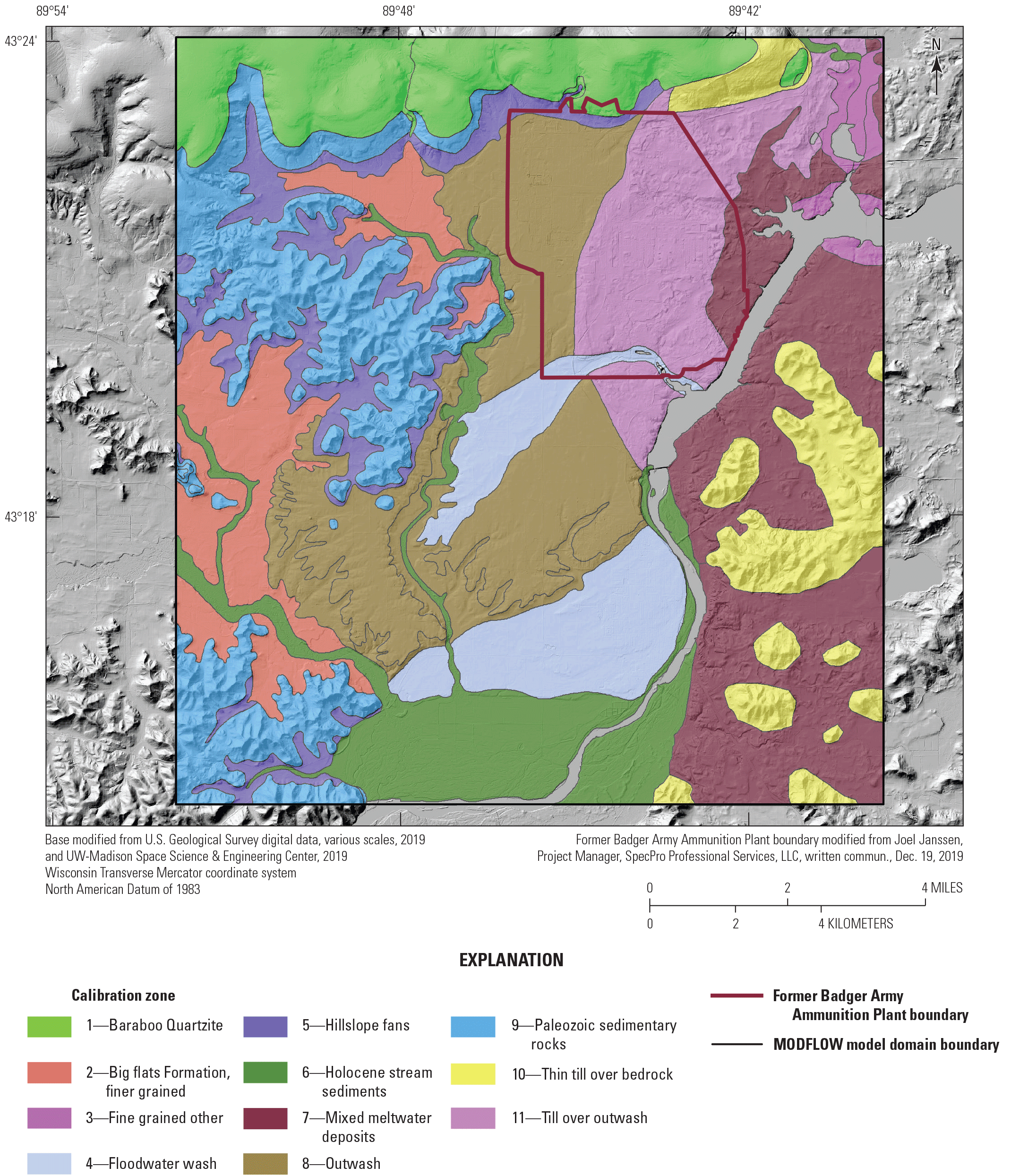
Calibration zones for the potential recharge inputs to the groundwater flow model.
References Cited
Allen, R.G., Pereira, L.S., Raes, D., and Smith, M., 1998, Crop evapotranspiration—Guidelines for computing crop water requirements: Rome, Food and Agriculture Organization of the United Nations, Irrigation and Drainage Paper 56: Food and Agriculture Organization of the United Nations Rome, 174 p. [Also available at https://www.fao.org/3/X0490E/x0490e00.htm#Contents.]
Fienen, M.N., Haserodt, M.J., Leaf, A.T., and Westenbroek, S.M., 2021, Central Sands lakes study technical report—Modeling documentation, app. C of Wisconsin Department of Natural Resources, Central Sands lakes study report—Findings & recommendations: Wisconsin Department of Natural Resources, 139 p., accessed February, 2023 at https://pubs.er.usgs.gov/publication/70220879.
Jin, S., Homer, C., Yang, L., Danielson, P., Dewitz, J., Li, C., Zhu, Z., Xian, G., and Howard, D., 2019, Overall methodology design for the United States National Land Cover Database 2016 Products: Remote Sensing (Basel), v. 11, no. 24, p. 2971. [Also available at https://doi.org/10.3390/rs11242971.]
Nielsen, M.G., 2023, Soil-Water-Balance (SWB) model archive used to simulate potential annual recharge for the former Badger Army Ammunition Plant study area, Prairie du Sac, Wisconsin, 1980 to 2020: U.S. Geological Survey data release, https://doi.org/10.5066/P9S2IDV0.
Soil Survey Staff, 2018, Gridded soil survey geographic (gSSURGO) database: Natural Resources Conservation Service web page, accessed September 5, 2019, at https://www.nrcs.usda.gov/resources/data-and-reports/description-of-gridded-soil-survey-geographic-gssurgo-database.
Thornthwaite, C.W., and Mather, J.R., 1957, Instructions and tables for computing potential evapotranspiration and the water balance: Publications in Climatology, v. 10, no. 3, p. 1–104, accessed February 2023 at https://www.wrc.udel.edu/wp-content/publications/ThornthwaiteandMather1957Instructions_Tables_ComputingPotentialEvapotranspiration_Water%20Balance.pdf.
Thornton, M.M., Shrestha, R., Wei, Y., Thornton, P.E., Kao, S., and Wilson, B.E., 2016. Daymet—Daily surface weather data on a 1-km grid for North America (ver. 3.0, July 2016): Oak Ridge National Laboratory Distributed Active Archive Center dataset, accessed November 10, 2020, at https://doi.org/10.3334/ORNLDAAC/1328.
Thornton, M.M., Shrestha, R., Wei, Y., Thornton, P.E., Kao, S., and Wilson, B.E., 2020, Daymet—Daily surface weather data on a 1-km grid for North America (ver. 4, December 2020): Oak Ridge National Laboratory Distributed Active Archive Center dataset, accessed June 3, 2021, at https://doi.org/10.3334/ORNLDAAC/1840.
U.S. Department of Agriculture, 2007, Hydrologic soil groups, chap. 7 of Hydrology, pt. 630 of National engineering handbook: U.S. Department of Agriculture, Natural Resources Conservation Service, 14 p. accessed June 1, 2021, at https://directives.sc.egov.usda.gov/OpenNonWebContent.aspx?content=22526.wba.
U.S. Geological Survey [USGS], 2019, USGS NED 1/3 arc-second n44w090 1 x 1 degree IMG 2019: U.S. Geological Survey dataset, accessed October 28, 2019, at https://www.usgs.gov/programs/national-geospatial-program/national-map.
University of Wisconsin–Madison, 2019a, Columbia, in UW–Madison Space Science & Engineering Center file repository: University of Wisconsin-Madison, Space Science & Engineering Center dataset, accessed October 30, 2019, at https://bin.ssec.wisc.edu/pub/wisconsinview/lidar/. [Columbia County data directly accessible at https://bin.ssec.wisc.edu/pub/wisconsinview/lidar/Columbia/.]
University of Wisconsin–Madison, 2019b, Sauk, in UW–Madison Space Science & Engineering Center file repository: University of Wisconsin-Madison, Space Science & Engineering Center dataset, accessed October 30, 2019, at https://bin.ssec.wisc.edu/pub/wisconsinview/lidar/. [Sauk County data directly accessible at https://bin.ssec.wisc.edu/pub/wisconsinview/lidar/Sauk/.]
Westenbroek, S.M., Engott, J.A., Kelson, V.A., and Hunt, R.J., 2018, SWB version 2.0—A soil-water-balance code for estimating net infiltration and other water-budget components: U.S. Geological Survey Techniques and Methods, book 6, chap. A59, 118 p., accessed January 1, 2019, at https://doi.org/10.3133/tm6A59.
Westenbroek, S.M., Kelson, V.A., Dripps, W.R., Hunt, R.J., and Bradbury, K.R., 2010, SWB—A modified Thornthwaite-Mather soil-water-balance code for estimating groundwater recharge: U.S. Geological Survey Techniques and Methods, book 6, chap. A31, 60 p. [Also available at https://doi.org/10.3133/tm6A31.]
Appendix 3. Development of Bedrock Surface and Hydrostratigraphic Zones
Depth to Bedrock
Determining the top of the bedrock surface was done using data points including well logs, previous groundwater models, and contours representing shallow bedrock where either Paleozoic sedimentary rocks or Precambrian rocks in the Baraboo Hills are at or near the land surface. Descriptions of the pre-glacial Wisconsin River Valley in Carson and others (2019) guided the interpolation of the surface from the available data points. The data sources included the bedrock surface for the Columbia County flow model (Gotkowitz and others, 2021), drilling records from SpecPro Professional Services, LLC (Joel Janssen, Project Manager, SpecPro Professional Services, LLC, written commun., February 1, 2021 [These data are not publicly available. Contact SpecPro Professional Services, LLC, for further information.]) for the U.S. Army Environmental Command wells on and near the site, geologic logs in the USGS Upper Midwest Water Science Center’s Madison office county well files for Sauk and Columbia Counties (files archived in Reeves and Corson-Dosch, 2023), previous groundwater studies in Sauk and Dane Counties (Gotkowitz and others, 2005; Gotkowitz and Zeiler, 2002, Clayton and Attig, 199763), and Wisconsin Department of Natural Resources county well reports for Dane, Columbia, and Sauk Counties (Wisconsin Department of Natural Resources, 2021).
A passive seismic survey led by Wisconsin Geological and Natural History Survey (WGNHS) staff (David Hart, WGNHS, written commun., December 15, 2020 [These data are not publicly available. Contact the WGNHS for further information.]) was used to fill in some areas in the middle of the former Badger Army Ammunition Plant (BAAP) site where no other bedrock data existed. Unlike traditional seismic methods that use an active sound source, passive seismic uses naturally occurring vibrations in the Earth to estimate the depths to subsurface contacts between materials, such as the bedrock surface. Although the method allows for rapid data collection, the results are generally less accurate, and errors in estimated depths can be 25 percent or greater (Chandler and Lively, 2016).
In the area between the Paleozoic bedrock outcrops on the east and west sides of the Wisconsin River, the surface was interpolated using ArcGIS’s TOPO to RASTER tools to create a hydrologically correct pre-glacial river valley cut into the surrounding bedrock. Carson and others (2019) present evidence that in pre-glacial times the river that flowed through this valley flowed towards the east, rather than towards the west as the Wisconsin River currently does. The set of bedrock surface data points (fig. 3.1) was augmented with control points to keep the TOPOGRID interpolation consistent with the shape of a river valley (with a defined thalweg and no internally draining depressions), and contours of the current bedrock surface outcrops. In total, there were 319 well records from the Sauk County groundwater work by Gotkowitz and Zeiler (2002), 164 Wisconsin Department of Natural Resources well records (Wisconsin Department of Natural Resources, 2021), 79 U.S. Army Environmental Command monitoring wells from SpecPro Professional Services, LLC (Joel Janssen, Project Manager, SpecPro Professional Services, LLC, written commun., February 1, 2021), 35 WGNHS passive seismic points (David Hart, WGNHS, written commun., December 15, 2020), 25 WiscLith logs (WGNHS, 2009; Reeves and Corson-Dosch, 2023), and 45 control points used. The locations of data points used for the interpolation is shown in figure 3.1.
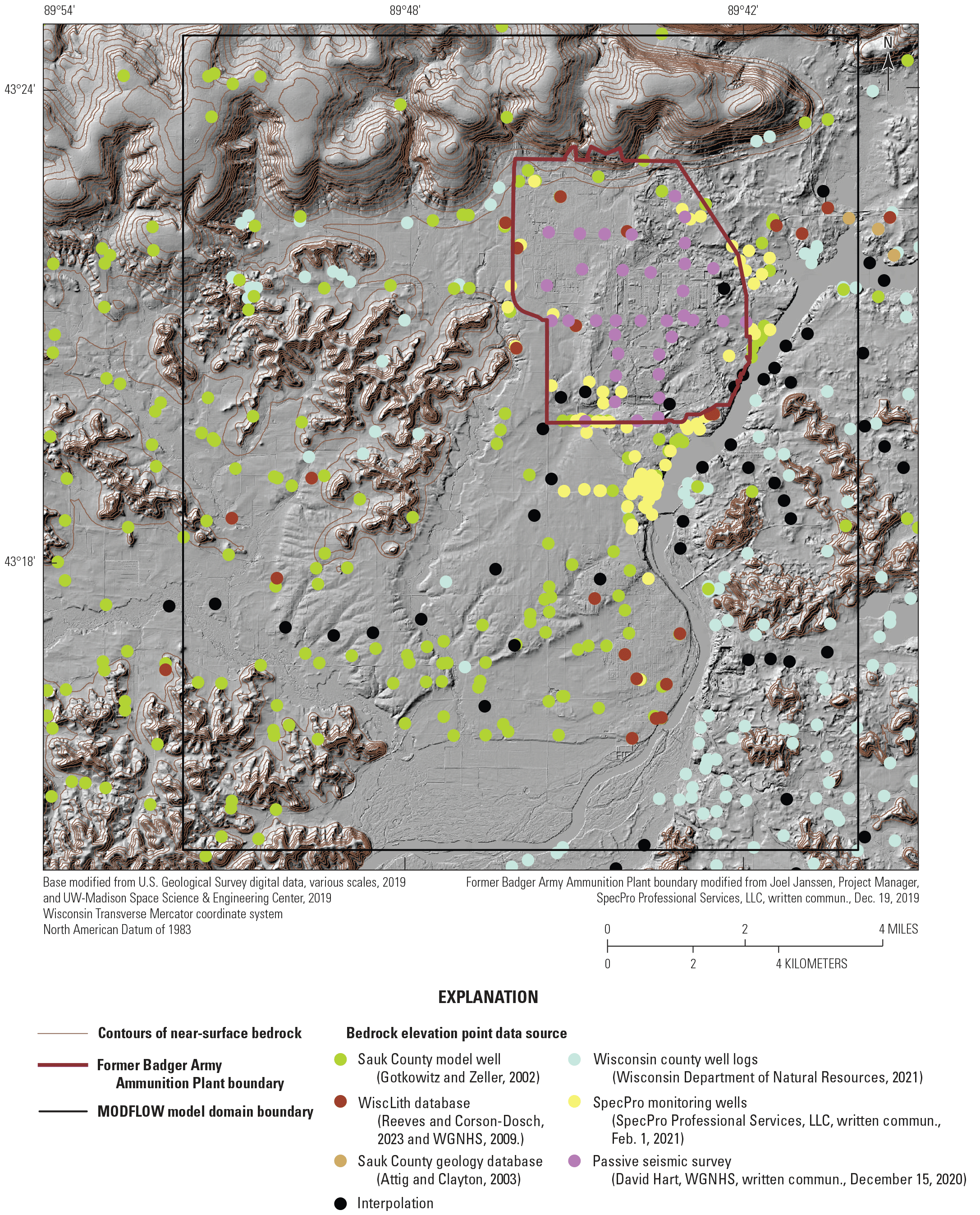
Data used in the interpolation of the depth to bedrock for the study area.
The depth to bedrock was calculated using a land surface grid and subtracting the newly defined bedrock surface combined with an assumed shallow soil zone above the Baraboo Hills and the Paleozoic bedrock hills on either side of the Wisconsin River. The shallow soil zone was assumed to be 25 feet for these areas. The land surface grid was developed using lidar-based digital elevation models from Sauk, Columbia, and Dane Counties (U.S. Geological Survey, 2019; University of Wisconsin–Madison, 2019a,b71), which were combined into one seamless digital elevation model for the study area.
The depth to bedrock map (fig. 3.2) shows the pre-glacial river valley that flows under the former BAAP site. The bedrock is deepest in the northeast part of the study area (more than 300 ft), and ranges from 150 to 275 ft under the middle of the BAAP site.
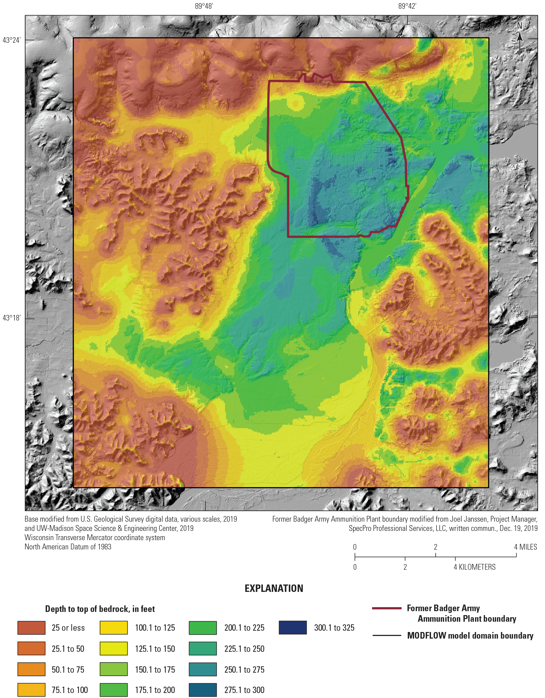
Depth to bedrock in the former Badger Army Ammunition Plant model study area.
Glacial Sediments Hydrostratigraphic Units
The hydrostratigraphic units used for the glacial sediments were derived by assigning textural characteristics to the sediments. Many well logs were available to use for categorizing the glacial units by textural characteristics, including logs from monitoring wells, private wells, and test holes on and near the site (SpecPro Professional Services, LLC, 2019) and Wisconsin Department of Natural Resources county well construction reports (Wisconsin Department of Natural Resources, 2021) and additional USGS wells logs (available in Reeves and Corson-Dosch,, 2023). Many of the wells with logs were next to each other but had varying total depths (many of the monitoring well locations had logs for four different depth wells). In such cases, the deepest, most-complete log was used. From 453 available well logs, 205 were eventually selected to create a three-dimensional hydrofacies (or textural classes) model for the glacial units.
Seven grain-size textural classes were used in the glacial unit classification: gravel, sand and gravel, sand, mixed-coarse, mixed-fine, silt and clay, and clay. The mixed-coarse and mixed-fine classes were used when an interval in the log contained a mix of coarse-grained and fine-grained sediments but either the coarse fraction or fine fraction was dominant. The other classes were used when the log interval description was relatively uniform.
The glacial sediments were assigned textural classes based on the descriptions in the well logs for each of the 10 model layers that the well intersected. For every well log location, the vertical model layering was converted into depth intervals below land surface. For each depth interval that the well intersects, the well log was assigned the appropriate textural class based on the textural description of sediments for the given depth interval. More well logs were available for the uppermost model layers than the deeper layers because fewer wells were drilled all the way to the bedrock surface. The top model layer, representing the shallowest glacial sediments, had 201 data points, and model layer 10, which represents sediments just above the top of the bedrock, had 111 data points.
To create the horizontal distribution of textural class zones for each model layer, the texture classes at each well point in each layer were converted to integer values, and an inverse weighted distance model was used to assign numeric values to the spaces between wells. The numeric values were converted back into a horizontal distribution of textural classes for each model layer. These were subsequently hand edited so that the distribution of sediment textures conformed better to the depositional history and mode of the glacial sediments in the study area.
The resulting zonation of textural classes is dominated by coarse-grained sediments, such as gravel, sand and gravel, and sand for most of the study area, which is a good representation of the outwash sand and gravel deposits that dominate the study area. The surficial sandy till of the Johnstown Moraine is above the uppermost model layer across much of the former BAAP site, and the underlying coarser-grained outwash deposits form most of the upper hydrofacies layer. The fine-grained silt and clay deposits are most common to the north of Lake Wisconsin east of the former BAAP site and to the northwest of the site. The glacial zones were combined with the shallow soil zones over the Paleozoic bedrock outcrops to complete the hydrostratigraphic zones for the top 10 model layers.
Bedrock Hydrostratigraphic Zones
The bedrock units in model layers 11–14 were divided into hydrostratigraphic zones based primarily on the stratigraphy of the formations in the study area. The uppermost and youngest sedimentary rocks (the Oneota Formation, St. Lawrence Formation, and Tunnel City Group) that were grouped into an “upper bedrock” hydrostratigraphic unit are all erosional remnants of the pre-glacial topography and do not form a substantial part of the groundwater flow system at the BAAP site. The Wonewoc Formation, Eau Claire Formation, and Mount Simon Formation compose the primary bedrock hydrostratigraphic units in the BAAP model. During the model calibration, two additional hydrostratigraphic zones of more highly weathered bedrock were put into the model layer 11 in the area next to the Baraboo Hills. The quartzite of the Baraboo Hills was not modeled and thus is not part of the hydrostratigraphy of the study area.
The surfaces for each bedrock formation were interpolated from point data from a range of sources. The Sauk County groundwater study by the WGNHS (Gotkowitz and others, 2005; Gotkowitz and Zeiler, 2002) contained 64 wells with elevations of the hydrogeologic units at depth in the study area, and 22 well logs from the Wisconsin WiscLith database (WGNHS, 2009) were available in the study area. Additionally, 129 well logs from the Wisconsin Department of Natural Resources county well reports for Dane, Columbia, and Sauk Counties (Wisconsin Department of Natural Resources, 2021) contained lithologic information used to delineate the sub-surface contacts between the units. The SpecPro Professional Services, LLC (2019) well log database contributed additional well logs. Descriptions of the Paleozoic bedrock units in Clayton and Attig (1990a, b)62 were used to interpret well drillers lithologic descriptions. Available data points for the contacts between the units were used to interpolate surfaces used to define the tops and bottoms of the Upper Bedrock unit, the Wonewoc Formation, the Eau Claire Formation, and the Mount Simon Formation.
The resulting distribution of hydrostratigraphic zones for the glacial and bedrock units in the Badger groundwater flow model (layers 1 through 14) are shown in the Aquifer Properties section of the main report text.
References Cited
Carson, E.C., Rawling, J.E., III, Daniels, J.M., and Attig, J.W., 2019, v. 543. The physical geography and geology of the driftless area—The career and contributions of James C. Knox, Geological Society of America Special Paper, 156 p. [Also available at https://doi.org/10.1130/SPE543.]
Chandler, V.W., and Lively, R.S., 2016, Utility of the horizontal-to-vertical spectral ratio passive seismic method for estimating thickness of Quaternary sediments in Minnesota and adjacent parts of Wisconsin: Interpretation (Tulsa), v. 4, no. 3, p. SH71–SH90. [Also available at https://doi.org/10.1190/INT-2015-0212.1.]
Clayton, L., and Attig, J.W., 1990a, Geology of Sauk County, Wisconsin: Wisconsin Geological and Natural History Survey Information Circular 67, 68 p., 2 plates, accessed September 16, 2021, at https://wgnhs.wisc.edu/catalog/publication/000317/resource/ic67.
Clayton, L., and Attig, J.W., 1990b, Geology of Sauk County, Wisconsin [GIS data; updated 2003]: Wisconsin Geological and Natural History Survey Information Circular 67–DI, accessed September 2021 at https://wgnhs.wisc.edu/catalog/publication/000317.
Clayton, L., and Attig, J.W., 1997, Pleistocene geology of Dane County, Wisconsin (ver. 2) [GIS data]: Wisconsin Geological and Natural History Survey Bulletin 95–DI, accessed September 2021 at https://wgnhs.wisc.edu/catalog/publication/000119.
Gotkowitz, M.B., Leaf, A.T., and Sellwood, S.M., 2021, Hydrogeology and simulation of groundwater flow in Columbia County, Wisconsin: Wisconsin Geological and Natural History Survey Bulletin 117, 51 p., accessed September 2022 at https://wgnhs.wisc.edu/catalog/publication/000985.
Gotkowitz, M.B., and Zeiler, K.K., 2002, Water-table elevation map of Sauk County, Wisconsin: Wisconsin Geological and Natural History Survey Miscellaneous Map 55, 1 sheet, scale 1:100,000, 1 p., accessed September 2021 at https://wgnhs.wisc.edu/catalog/publication/000457/resource/m145.
Gotkowitz, M.B., Zeiler, K.K., Dunning, C.P., Thomas, J.C., and Lin, Y., 2005, Hydrogeology and simulation of groundwater flow in Sauk County, Wisconsin: Wisconsin Geological and Natural History Survey Bulletin 102, 43 p., accessed September 2021 at https://wgnhs.wisc.edu/pubshare/B102.pdf.
Reeves, H.W., and Corson-Dosch, N.T., 2023, Groundwater model archive for the former Badger Army Ammunition Plant, Wisconsin: U.S. Geological Survey data release, https://doi.org/10.5066/P9LNRILT.
SpecPro Professional Services, LLC, 2019, Remedial investigation/feasibility study for site-wide groundwater at the former Badger Army Ammunition Plant, Baraboo, Wisconsin: publisher, 717 p., accessed March 2020 at https://cswab.org/wp-content/uploads/2020/05/Badger-Army-Site-Wide-Groundwater-RIFS-Study-DRAFT-Nov-2019.pdf.
U.S. Geological Survey [USGS], 2019, USGS NED 1/3 arc-second n44w090 1 x 1 degree IMG 2019: U.S. Geological Survey dataset, accessed October 28, 2019, at https://www.usgs.gov/programs/national-geospatial-program/national-map.
University of Wisconsin–Madison, 2019a, Columbia, in UW–Madison Space Science & Engineering Center file repository: University of Wisconsin-Madison, Space Science & Engineering Center dataset, accessed October 30, 2019, at https://bin.ssec.wisc.edu/pub/wisconsinview/lidar/. [Columbia County data directly accessible at https://bin.ssec.wisc.edu/pub/wisconsinview/lidar/Columbia/.]
University of Wisconsin–Madison, 2019b, Sauk, in UW–Madison Space Science & Engineering Center file repository: University of Wisconsin-Madison, Space Science & Engineering Center dataset, accessed October 30, 2019, at https://bin.ssec.wisc.edu/pub/wisconsinview/lidar/. [Sauk County data directly accessible at https://bin.ssec.wisc.edu/pub/wisconsinview/lidar/Sauk/.]
Wisconsin Department of Natural Resources, 2021, The Groundwater Retrieval Network: Wisconsin Department of Natural Resources, Drinking Water and Groundwater Program website, accessed February 9, 2021, at https://dnr.wisconsin.gov/topic/Groundwater/GRN.html.
Wisconsin Geologic and Natural History Survey, 2009, wiscLITH—A digital lithologic and stratigraphic database of Wisconsin geology (ver. 3): Wisconsin Geologic and Natural History Survey database, accessed February 10, 2020, at https://wgnhs.wisc.edu/catalog/publication/000889/resource/wofr200903.
Appendix 4. Target Sets and Calibration Results
Table 4.1.
Observation sets and PEST observation groups.| Set number | Observation set | Source | PEST observation groups | Number of observations | Figure number for calibration results plot |
|---|---|---|---|---|---|
| 1 | Synoptic hydraulic heads | Existing data from SpecPro1 and National Water Information System database (U.S. Geological Survey, 2021). | synoptic a | 643 | Figure 4.7 |
| synoptic d | 169 | ||||
| synoptic e | 49 | ||||
| synoptic f | 4 | ||||
| synoptic nwis | 11 | ||||
| 2 | Hydraulic head and river stage differences | Existing data from SpecPro1 and river stages from National Water Information System database (U.S. Geological Survey, 2021). | rivdiff | 253 | Figure 4.8 |
| 3 | Timeseries hydrographs | Existing data from SpecPro1 | timeseries | 390 | Figure 4.9 |
| 4 | Seasonal timeseries hydrographs | Existing data from SpecPro1 | seasonal | 119 | Figure 4.10 |
| 5 | Water level rise (2015–19 and 2016–20) | Existing data from SpecPro1 | rise1 | 36 | Figure 4.11 |
| rise2 | 35 | ||||
| 6 | Water level response to 2005 MIRM pumping | Existing data from SpecPro1 | mirm | 61 | Figure 4.12 |
| 7 | Lateral gradient (magnitude and direction) of well triplets | Existing data from SpecPro1 | latgrad | 338 | Figure 4.13 |
| latdirec | 338 | ||||
| 8 | Vertical gradients across well nests | Existing data from SpecPro1 | vertgrad1 | 1 | No figure. |
| vertgrad2 | 1 | ||||
| vertgrad3 | 1 | ||||
| 9 | Minipiezometer observations | National Water Information System database (U.S. Geological Survey, 2021) | minipiez | 6 | Figure 4.14 |
| 10 | MODPATH particles matching to simple plume polygons | Existing data from SpecPro1 | modpath | 3 | No figure. |
| 11 | Discharge for Otter Creek | National Water Information System database (U.S. Geological Survey, 2021) | ottercreek | 4 | Figure 4.16 |
| 12 | MODPATH particles emitted from source areas that enter upper bedrock | Existing data from SpecPro1 | greater_than_count | 3 | No figure. |
| rock_dist | 3 | ||||
| 13 | Synoptic hydraulic heads per plume areas | Existing data from SpecPro1 | pbg_heads | 2,051 | Figure 4.17 |
| dbg_heads | 1,061 | ||||
| cen_heads | 721 | ||||
| 14 | Lateral gradient (magnitude and direction) for selected stress periods | Existing data from SpecPro1 | expgrad | 63 | Figure 4.18 |
| expdirec | 63 | ||||
| NA | Total observations | NA | NA | 6,427 | NA |
Set 1—Synoptic Hydraulic Heads
Set 1 consists of hydraulic heads (groundwater elevations) from the U.S. Geological Survey National Water Information System database (U.S. Geological Survey, 2021) and U.S. Army Environmental Command monitoring wells across the site for 11 of the model stress periods representing water levels in September in 1989, 1993, 1996, 2002, 2006, 2008, 2010, 2013, 2016, 2018, and 2020. The set 1 hydraulic heads were used to check the ability of the model to match the spatial distribution of heads across the site. Wells in this set had at least 26 years of data with no gaps in data exceeding 2 years.
In total, 194 wells were used for these synoptic observations (fig. 4.1). Not every well has an observation for all 11 selected stress periods. The observations are divided into the lettered horizons used in previous reports on the site (as described in app. 1), and there are 148 A-wells, 34 D-wells, 10 E-wells, 1 F-well, and 1 NWIS well.
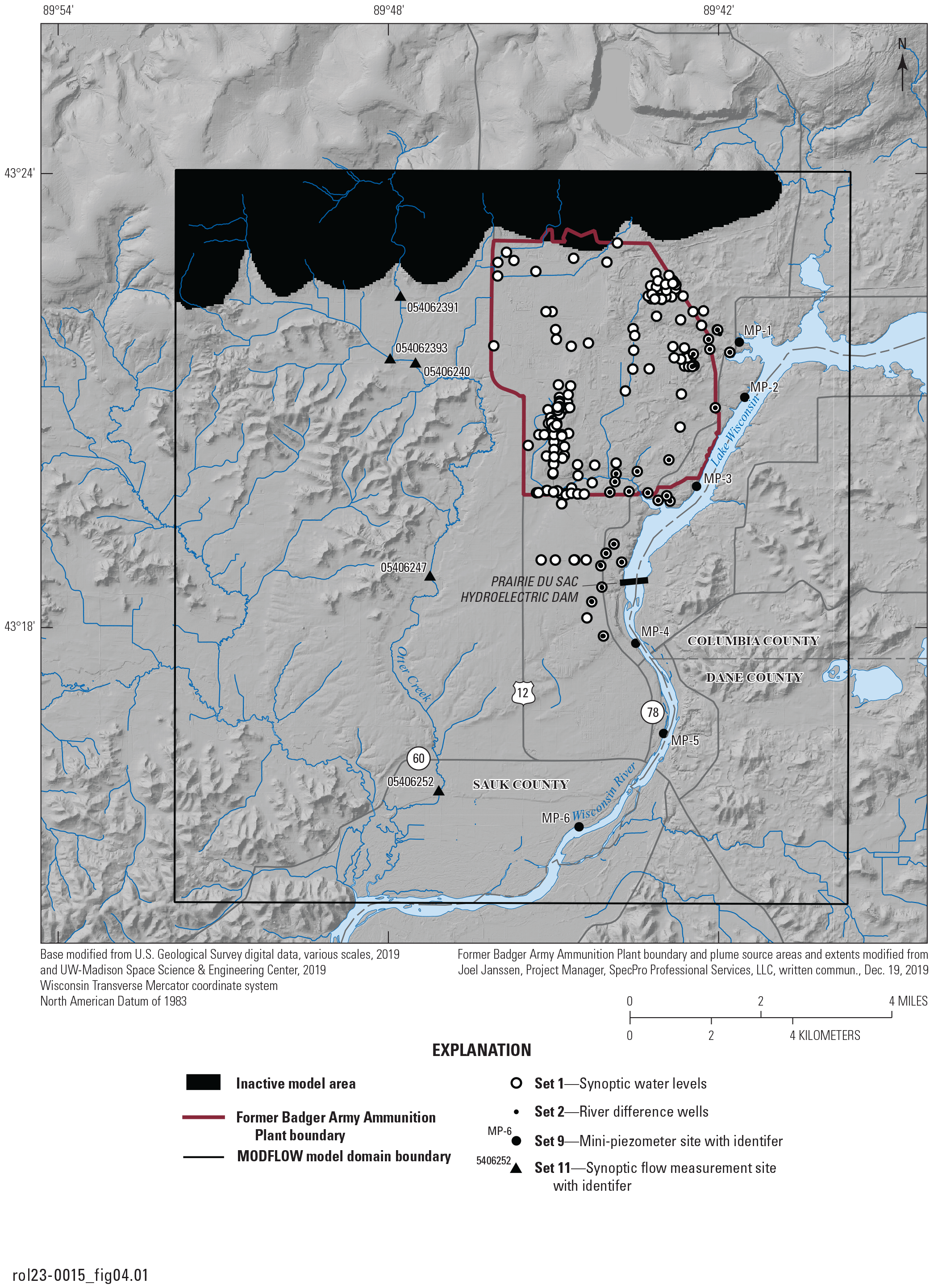
Well locations for the set 1 synoptic hydraulic head observations, set 2 hydraulic head and river stage observations, set 9 mini-piezometers, and set 11 Otter Creek discharge measurement locations.
Set 2—Hydraulic Head and River Stage Difference
The Prairie du Sac hydroelectric dam on the Wisconsin River affects the groundwater flow patterns in the model area. Far upstream from the dam, the hydraulic heads are higher than the river stage and groundwater flows from the aquifer to the river. Immediately upstream from the dam, the situation reverses, and the river stage tends to be higher than the hydraulic heads in the nearby aquifers. Downstream from the dam, there is a strong reversal with hydraulic heads greater than the river stage again. To focus on this general pattern, observation set 2 was developed to isolate the difference between the observed hydraulic heads in wells near the Wisconsin River and the long-term average river stage (calculated from water elevations in dataset provided by Amanda Blank, Site Manager, Hydroelectric & Gas Generation, Alliant Energy, written commun., December 29, 2020 [These data are not publicly available. Contact Alliant Energy for further information.]) above and below the dam (fig. 4.1).
Set 3—Full Simulation Period Timeseries Hydrographs for 13 Wells and Annual Water Level Changes
Observation set 3 was developed to check if the flow model can match observed groundwater levels changes over time at the site. For this set, the change in the observed water level from one stress period to the next was estimated from the observed water levels. The observations were interpolated to estimate the hydraulic head at the end of each stress period. Only sequential stress periods with observations close enough in time for reasonable interpolation were used as observations. Set 3 wells had more than 20 years of record during the model period and were selected to provide coverage across the model domain. Figure 4.2 shows the location of the set 3 wells. This observation set can be very useful because it does not focus on the observed values for hydraulic head, rather it looks at the changes in these values; moreover, the ability of the model to react appropriately to changes in the system can be evaluated (for more discussion on this type of observation, see Westenbroek and others, 2012). These transient hydrographs were used to help constrain the recharge and specific yield parameters.
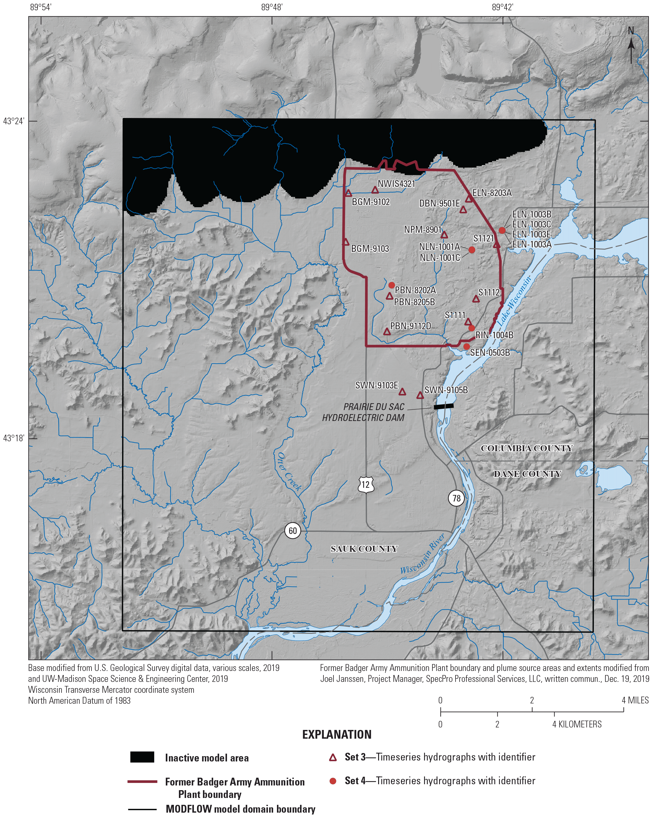
Well locations for the set 3 and set 4 timeseries wells.
Set 4—2017–20 Timeseries Hydrographs for Nine Wells and Quarterly Water Level Changes
To focus on recent groundwater level changes at the site and improve chances of calibrating recharge and storage, observation set 4 was developed. Set 4 focuses on the quarterly water level changes during the last several stress periods of the model. As the model stops at the end of the 2020 water year, this set encompasses 15 timesteps, each 3 months long starting in January 2017 and ending on September 30, 2020. This set includes the change in groundwater level between quarters and the average groundwater elevation for that quarter based on all available measurements. This last group of stress periods are shorter and are aimed at capturing more of the short-term response of the system. Like set 3, the change in water level is used as the observed value. Figure 4.2 shows the location of the set 4 wells.
Set 5—2015–19 and 2016–20 Water Level Rise for 13 Wells
Observation set 5 was made to capture the overall rise in hydraulic heads observed in recent years. Two observation groups were made for 13 wells, the change in water levels from 2015 to 2019, and the change in water levels from 2016 to 2020 (fig. 4.3). This set is similar in concept to sets 3 and 4, but only the overall rise is used as the observation, not the stress-period to stress-period change.
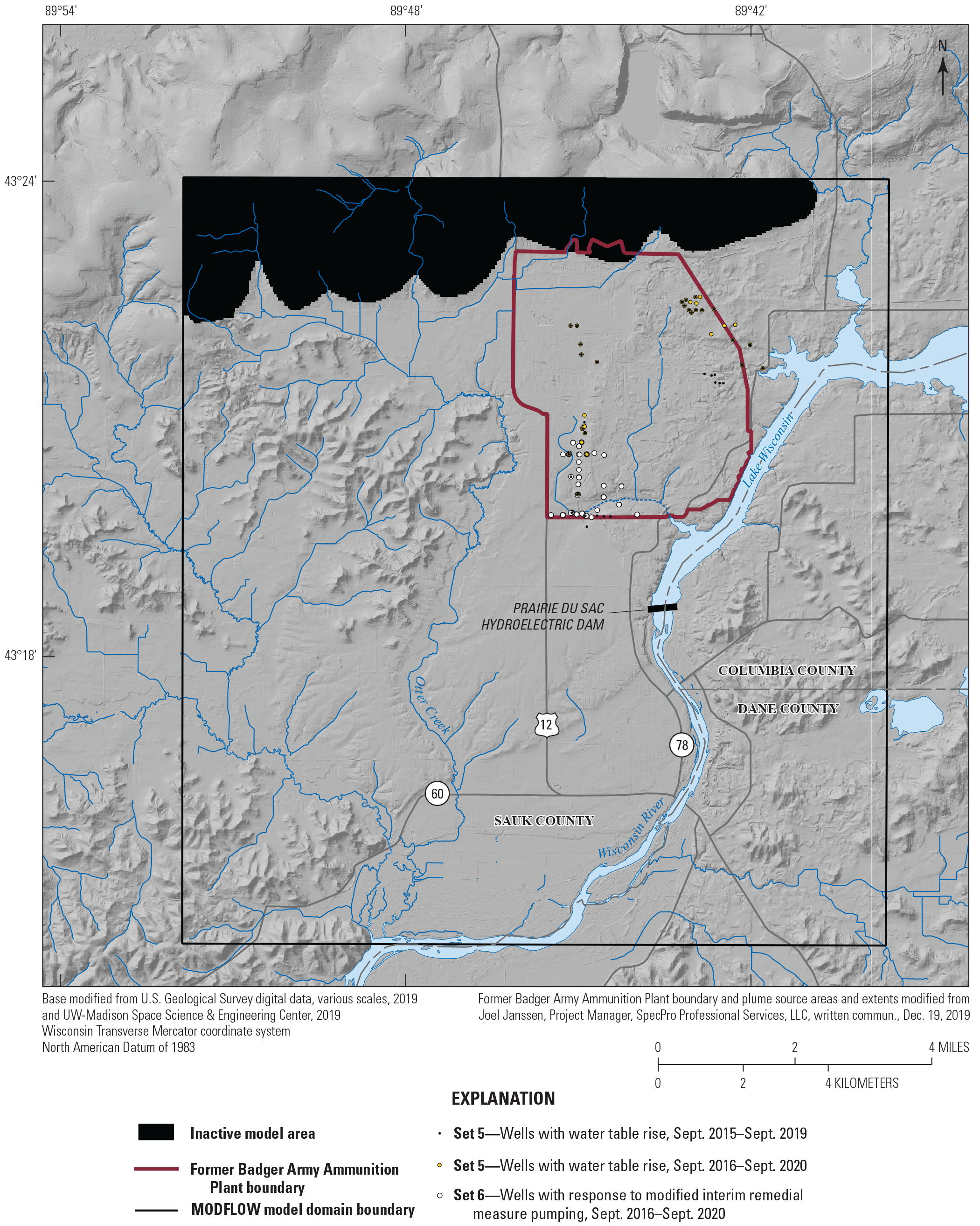
Well locations for the set 5 water level rise and set 6 modified interim remedial measure pumping responses.
Set 6—Change in Water Level in Response to Changes in Pumping During 2005 MIRM Pumping
In 2005, remediation operations changed at the site, and additional pumping wells were added to the modified interim remedial measure (MIRM). Not all the details of this change are available, but monthly reports around this time were used to estimate changes in pumping that were applied to the model from retirement of some and addition of other remedial wells toward the end of April 2005. Shorter stress periods from May through September 2005 were used to try to better capture these pumping changes. Observation set 6 was developed to better estimate transmissivity and storage properties near the pumping wells. This observation set uses wells that capture changes in observed hydraulic heads near the MIRM remedial system (fig. 4.3).
Set 7—Lateral Gradients from Triplets of Wells, Magnitude, and Direction
Target set 7 was made using 26 triplets of wells across the model domain and stress periods, yielding 338 lateral gradient calculations. The triplets were calculated for stress periods corresponding to years from 1988 to 2020. The stress periods used for each triplet of wells depended on the observations available and varied between triplets. This target set is unique in two ways: it consists of two targets, the gradient magnitude and direction, and the target is not associated with a single well location but with the centroid of the associated triplet of wells (fig. 4.4). After experimenting with this observation set, the observations were quite noisy and hard to interpret. A related observation set with well triplets spaced further apart, in an attempt to estimate more stable gradients, was developed as set 14. Observations of this type were discussed by Ruskauff and Rumbaugh (1996).
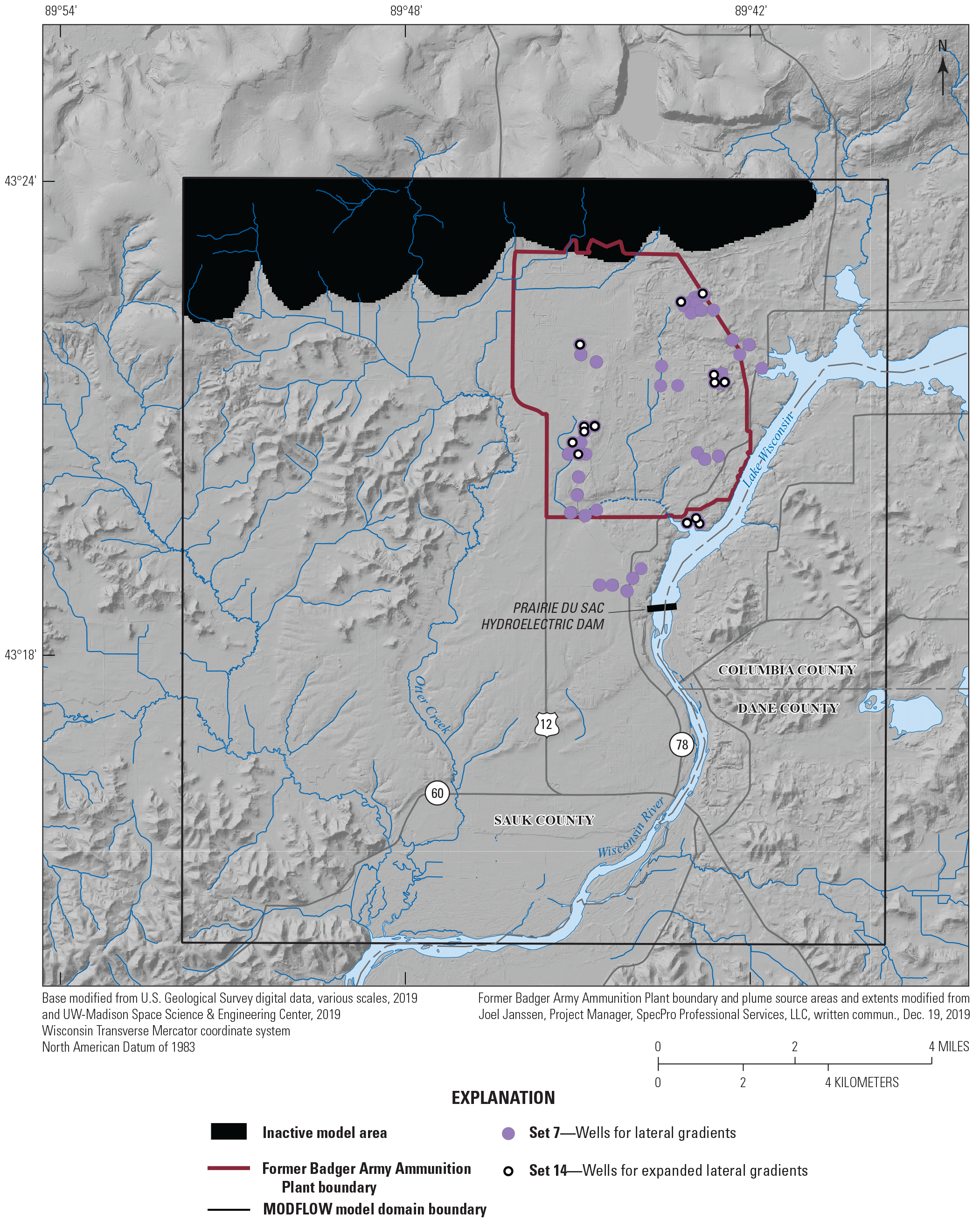
Well locations for the set 7 lateral gradient triplets and set 14 expanded lateral gradient triplets.
Set 8—Vertical Gradients Across Nested Well Pairs
Observation set 8 consists of three separate groups of vertical gradients calculated for the model domain. These three groups correspond to different depth comparisons using the site well letter system discussed in appendix 1. This target sets includes gradients between B to C wells (within glacial gradient, 99 observations at the end of water years 2007, 2015, and 2020), D to E wells (from deep glacial to shallow bedrock, 9 observations at the end of water years 2007, 2015, and 2020), and D to F wells (from deep glacial to deep bedrock, 2 observations at the end of water years 2015 and 2020). Each vertical gradient observation involves a shallow and a deep well, either from a nested pair or closely neighboring wells. The value of the vertical gradient is reported positive downward with the direction characterized in one of three ways: “UP” if the vertical gradient is from deep to shallow and equals or exceeds –0.001 foot per foot, “DOWN” if the vertical gradient is from shallow to deep and equals or exceeds +0.001 foot per foot, or “FLAT” if the absolute value of the vertical gradient, regardless of direction, is less than 0.001 foot per foot. The locations of the wells used for these vertical gradient targets are shown in figure 4.5.
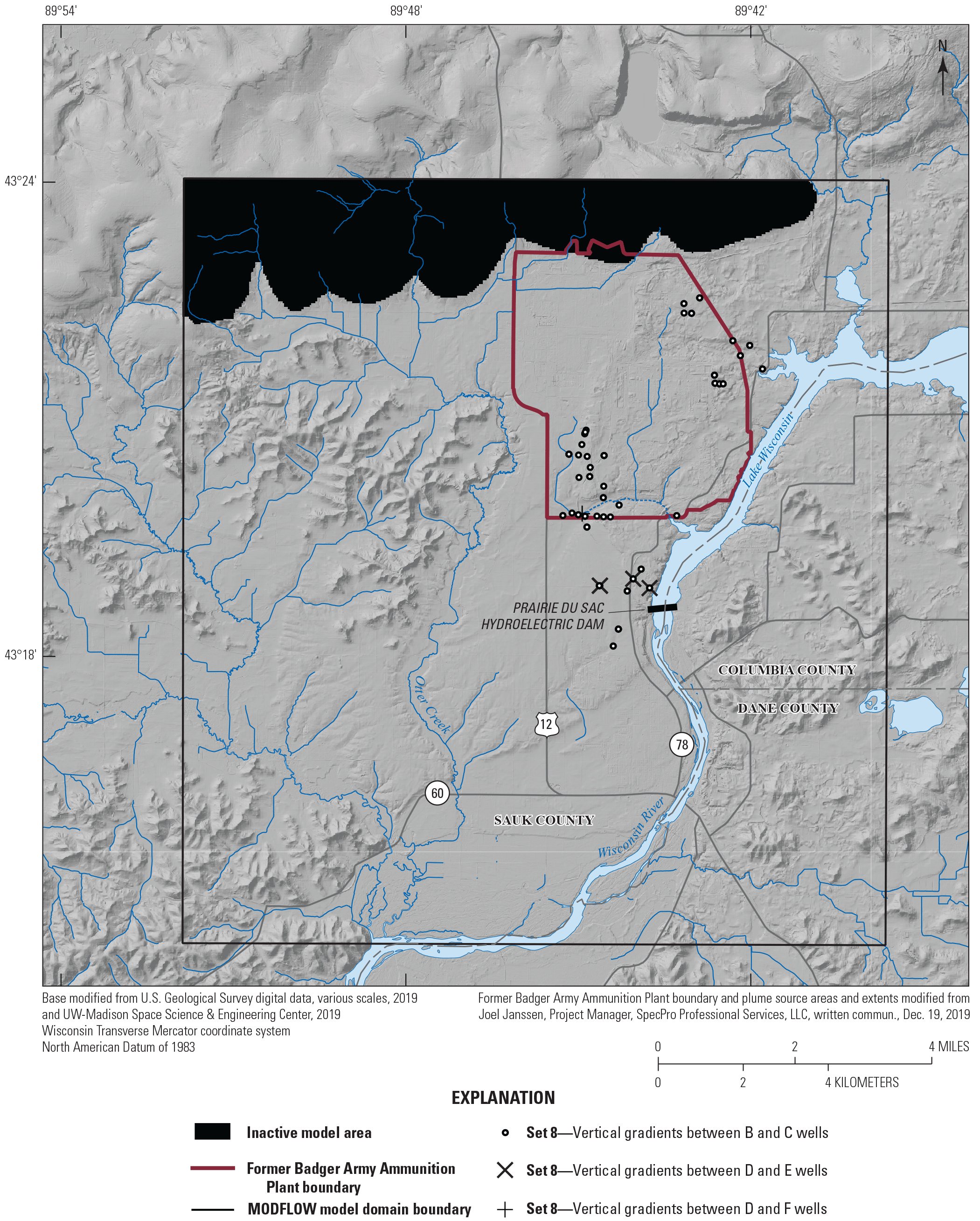
Well locations for the set 8 vertical gradients across nested pairs of wells.
Set 9—Mini-Piezometer Measured Vertical Gradients
Target set 9 consists of the six mini-piezometer readings taken along the Wisconsin River as described in the “Field Data Collection” section. A vertical gradient magnitude was calculated from these field data and indicates if the river is gaining or losing at the measurement point. The modeled head difference between the groundwater and river was then compared to the measured head difference at the mini-piezometer. The mini-piezometer locations are shown in figure 4.1.
Set 10—MODPATH Particles Falling into Simple Plume Polygons
Because most of the observations were derived from the set observation wells, many of the observation sets are expected to be correlated. To bring in another data type for calibration, MODPATH (Pollock, 2016) was used to simulate how particles move with the flowing groundwater for the simulation period from 1984 to 2020. Particle locations were compared to the generalized plume shapes modified from the plumes mapped by SpecPro Professional Services, LLC (2019). For the deterrent burning ground (DBG) and central plumes, 8 and 24 particles, respectively, were released in the source areas. For the propellant burning ground (PBG) plume, 25 particles were released in the source area and an additional 12 particles were released near the site boundary downgradient from the MIRM remediation wells. These downgradient particles were used to ensure the lower part of the plume was tested because the particles near the source area could be captured by the MIRM wells. At each stress period, the distance from every particle to the boundary of its corresponding simplified plume polygon was computed and summed to give three observations for the PBG, DBG, and central plumes. Any particles within the simplified plume polygon were assigned a distance of zero, and the target observed value for this observation set was zero for all particles within the plumes. For some realizations, particles from the central plume continue downgradient farther than the interpolated plume, and these particles were not used in the distance calculation. The excluded particles were identified by comparing the north-south location of the particle to the southern edge of the center plume polygon and excluding those that travel farther south than the polygon.
Set 11—Discharge for Otter Creek
Traditionally, groundwater flow models were calibrated to several sets of flow measurements from surface water features within the model domain; however, the Badger Army Ammunition Plant model has very few surface-water features within its domain other than the Wisconsin River and Otter Creek. The discharge measurement locations for synoptic streamflow data collected for this study are shown in figure 4.1. Differences are calculated as the change in streamflow observed between upper sites 54062393 and 5406247 and lower sites 5406247 and 5406252 (fig. 4.1). A total of four streamflow difference targets were used and included an upper and lower difference calculated from the July 13, 2020, and October 20, 2020, synoptic data.
Set 12—MODPATH Particles Emitted from Source Areas that Enter Upper Bedrock
Observations at the site generally show not detected or low concentrations of chemicals of concern in the upper bedrock monitoring wells, but if contaminants have entered the bedrock, remedial actions by pump-and-treat or bioremediation could be hampered by slow transport out of the bedrock. Therefore, to try to prevent the groundwater flow model from predetermining a best-case scenario with no concentration reaching the bedrock or a worst-case scenario with a great deal of flow moving through the bedrock, observations to count the number of particles reaching the bedrock for each plume and to record the closest distance from particles to the bedrock for each plume were implemented for set 12. The weight for the closest distance to the bedrock observation was set to zero, so this observation is a convenience allowing the user to quickly find that information. The count for particles to the bedrock observation was set to a target of greater than four particles. If greater than four particles reach the bedrock for any plume, the observation does not enter the PEST calculations. If less than four particles reach the bedrock for any plume, a slight penalty is added to the PEST calculation to try and have at least some particles reach the top of the bedrock.
Set 13—Synoptic Hydraulic Heads Focused on Plume Areas
This target set consists of a set of September water level measurements for each of the three plume areas (DBG, PBG, and central plumes). The measurements are from 1988 to 2020 for the DBG and PBG and 1988 to 2019 for the central plume. The wells used in this set are shown in figure 4.6. This observation set overlaps with the synoptic heads from across the site, set 1, but it is convenient to have a separate target group focused on the plume areas because these are the crucial areas for the model.
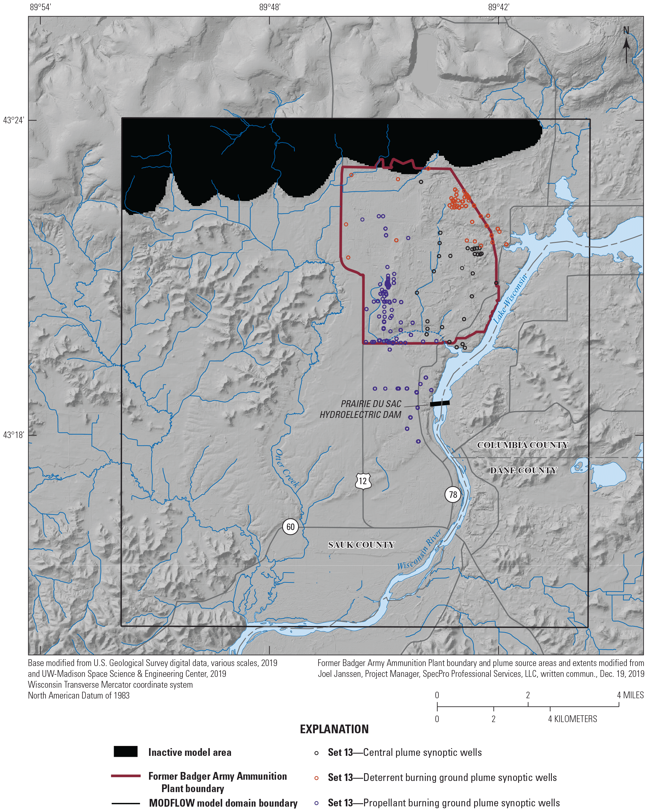
Well locations for the set 13 synoptic head observations by plume area.
Set 14—Lateral Gradient Triplets for a Subset of Wider Spaced Wells
This observation set is like set 7, except the triplet of wells used to calculate the lateral gradient magnitude and direction are farther apart than in set 7. Set 7 well triplets were typically on the order of 1,000-foot spacing, whereas set 14 was assigned to capture site-wide gradients because the closer spacing in set 7 proved to be a noisy dataset during the calibration. Set 14 consists of 63 observations calculated from 17 well triplets (fig. 4.4).
Model Calibration Results for the 14 Target Sets
The model was considered calibrated when the simulated and observed hydraulic heads, gradients, and fluxes closely matched for the various observation target sets, and the model parameters had reasonable values relative to literature ranges. This section provides a summary of the calibration fit for the 14 observation sets.
Sets representing synoptic data (sets 1, 2, 5, 6, 7, 9, 11, 13, and 14) had simulated and observed values plotted against each other with a 1:1 line (indicating a perfect fit); these sets are shown in figures 4.7, 4.8, 4.11, 4.12, 4.13, 4.14, 4.16, 4.17, and 4.18, respectively. A mean error and absolute mean error were included on each plot. The mean error indicates if there is bias high or low in the modeled values relative to the observed data. The mean absolute error provides information on the overall magnitude of these differences, a measure of fit. In general, points fell on or near the 1:1 line with scatter above and below the line for most of the observation sets. Mean errors were generally less than 1 foot, and mean absolute errors were generally less than 3 feet for observation sets representing hydraulic heads. Overall, synoptic datasets showed reasonable fits in the set 1 synoptic heads (fig. 4.7), set 2 (fig. 4.8) and 9 (fig. 4.14) vertical gradients to the Wisconsin River, and set 13 synoptic heads (fig. 4.17) in the plume areas. Poorer fits were observed with the set 5 water level rises (fig. 4.11), set 6 MIRM response (fig. 4.12), set 7 (fig. 4.13; zero-weighted) and 14 (fig. 4.18) gradient direction and magnitude, and set 11 Otter Creek streamflow difference targets (fig. 4.16). The overall calibration produced reasonable results in areas near the plumes, which are the focus of the model, and was able to generally capture past transient events like the MIRM pumping and water level rises. The model did not do a good job capturing the overall flow dynamics of Otter Creek. Otter Creek is not near the plumes, so it was not a focus of the model calibration.
Sets representing timeseries data (sets 3 and 4) were plotted with the simulated and observed timeseries on one plot, and the change in water level between observation points on a second plot. These timeseries hydrographs are shown in subplots in figures 4.9 and 4.10. The model generally simulated the overall pattern of the observed timeseries datasets with some wells (for example, NWIS–4321–8944, PBN–9112D, and SWN–9105B) better simulated than others (for example, BGM–9102 and BGM–9103). Although the model captured the overall patterns (rising or declining water levels), it often missed the timing slightly with the simulated values changing slightly ahead of the observed pattern. This is potentially due to the thick unsaturated zone that is not explicitly modeled in the groundwater model, meaning that recharge moves to the water table immediately after leaving the root zone. In reality, there could be a delay between recharge and a subsequent rise in the water table if that recharge must move through a thick unsaturated layer before reaching the water table.
The observation set 10 uses a metric to assess the paths of MODPATH particles originating in plume source area against the estimated plume footprint from the site water quality data. This metric cannot be displayed on a 1:1 plot and is best captured by observing the decline in phi (the sum of the square residuals) for the ensemble over the calibration (fig. 4.15). This decline represents pathlines that are better aligning with the plume footprint as the calibration progresses. Because understanding the groundwater flows near the plume is a key objective of this model, the improved pathline fits suggest that the calibrated ensemble is better able to meet this objective than the model before calibration.
For set 8, a summary approach is used for the final calibration target. For each well pair, the vertical gradient and DOWN, FLAT, UP designation is recorded in the set 8 output. Additionally, a summary score is used for any well where the simulated class differs from the observed class. A pair is given a score of 1, for example, if the observed vertical gradient is UP but the simulated is FLAT. If the difference is two classes, for example, the observed vertical gradient is UP but the simulated is DOWN, then the score for that well pair is set to 2. If the classes match, the score is set to −1. The score for all well pairs is then summed for each observation group within this set. The target value for the score was set to zero. Positive values for this set indicate that the individual well pairs should be checked for consistency with the directions of the observed vertical gradients. This observation set was not highly weighted in the calibration process but used as a secondary check on the progress of the model.
For set 12, for the base run, 2 particles reached the bedrock for the PBG plume and no particles reached the bedrock for the central or DBG plumes. Other realizations in the ensemble had as many as 20 particles that reached the bedrock for the PBG plume, and 6–10 particles reach the bedrock for the central and DBG plumes. The ensemble therefore provides different flow fields that on average meet calibration targets but have slightly different behavior and can be used in future transport modeling or design. The flow field meets the desired goal of not pre-supposing that the flow field will not carry contaminant to the bedrock nor does it place most of the contaminant in the bedrock which does not appear to be supported by field observations.
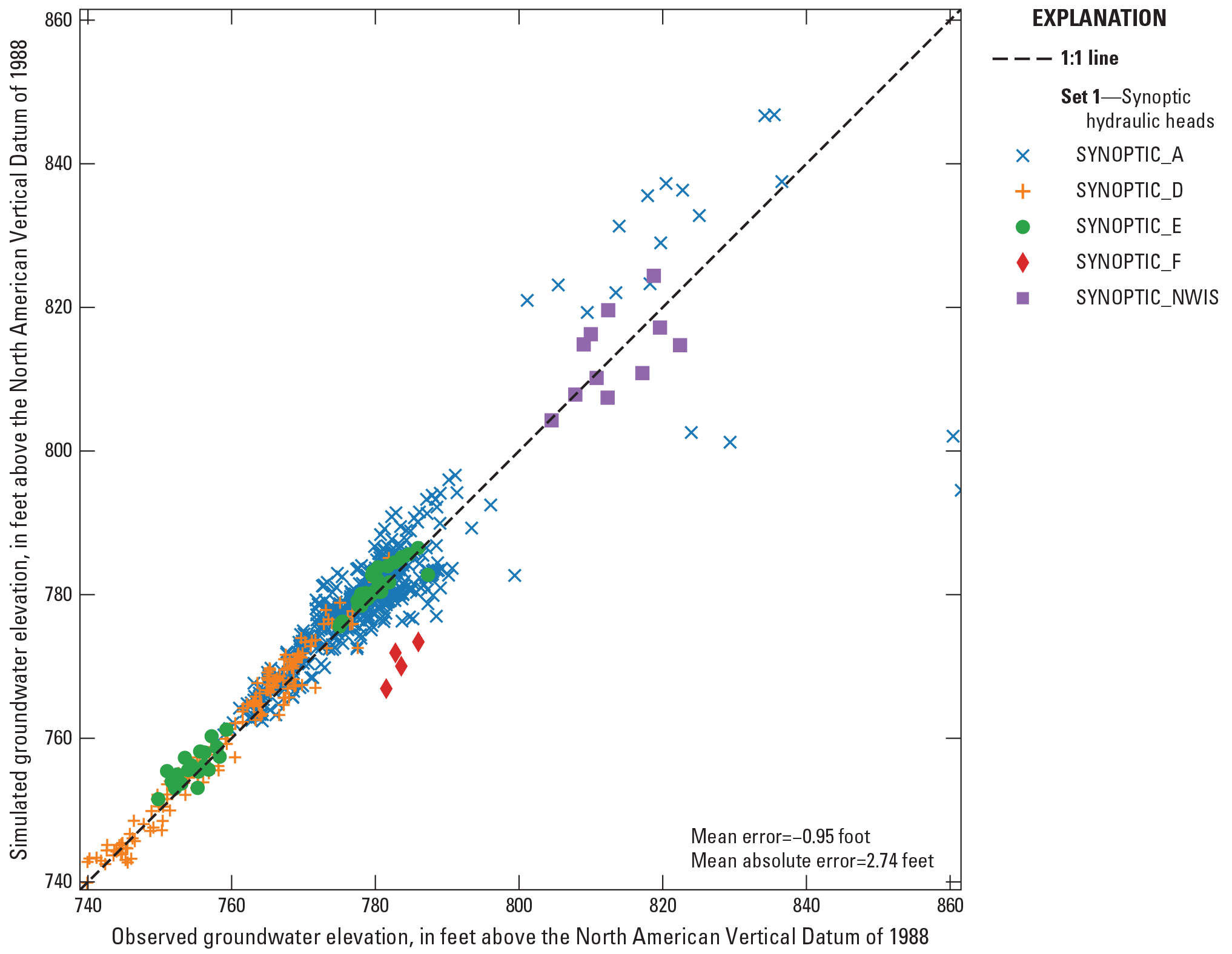
Observed and simulated hydraulic heads for the set 1 synoptic head (SYNOPTIC A, SYNOPTIC D, SYNOPTIC E, SYNOPTIC F, SYNOPTIC NWIS) observation group using the base model.
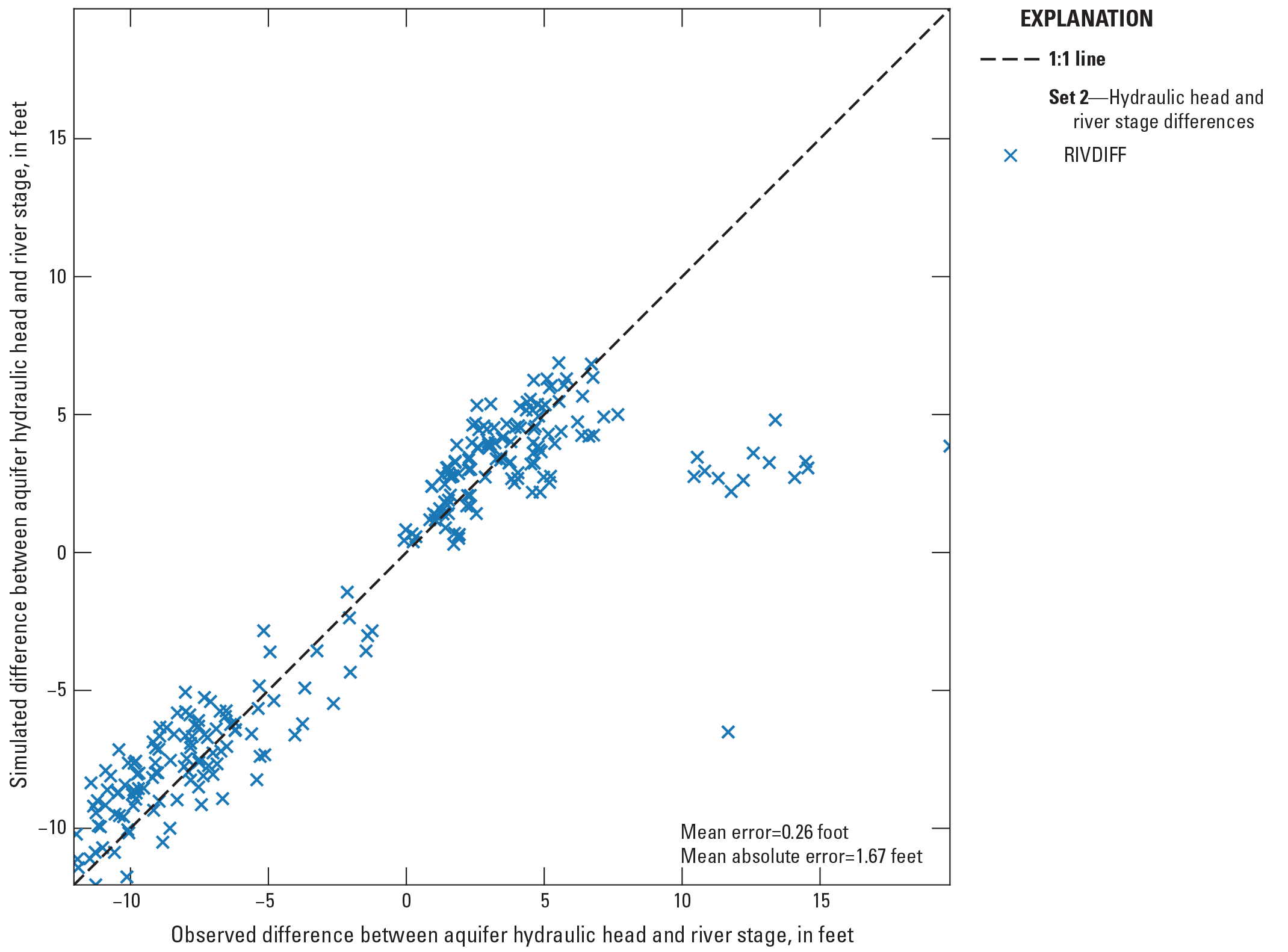
Observed and simulated hydraulic head difference for the set 2 river difference (RIVDIFF) observation group using the base model.
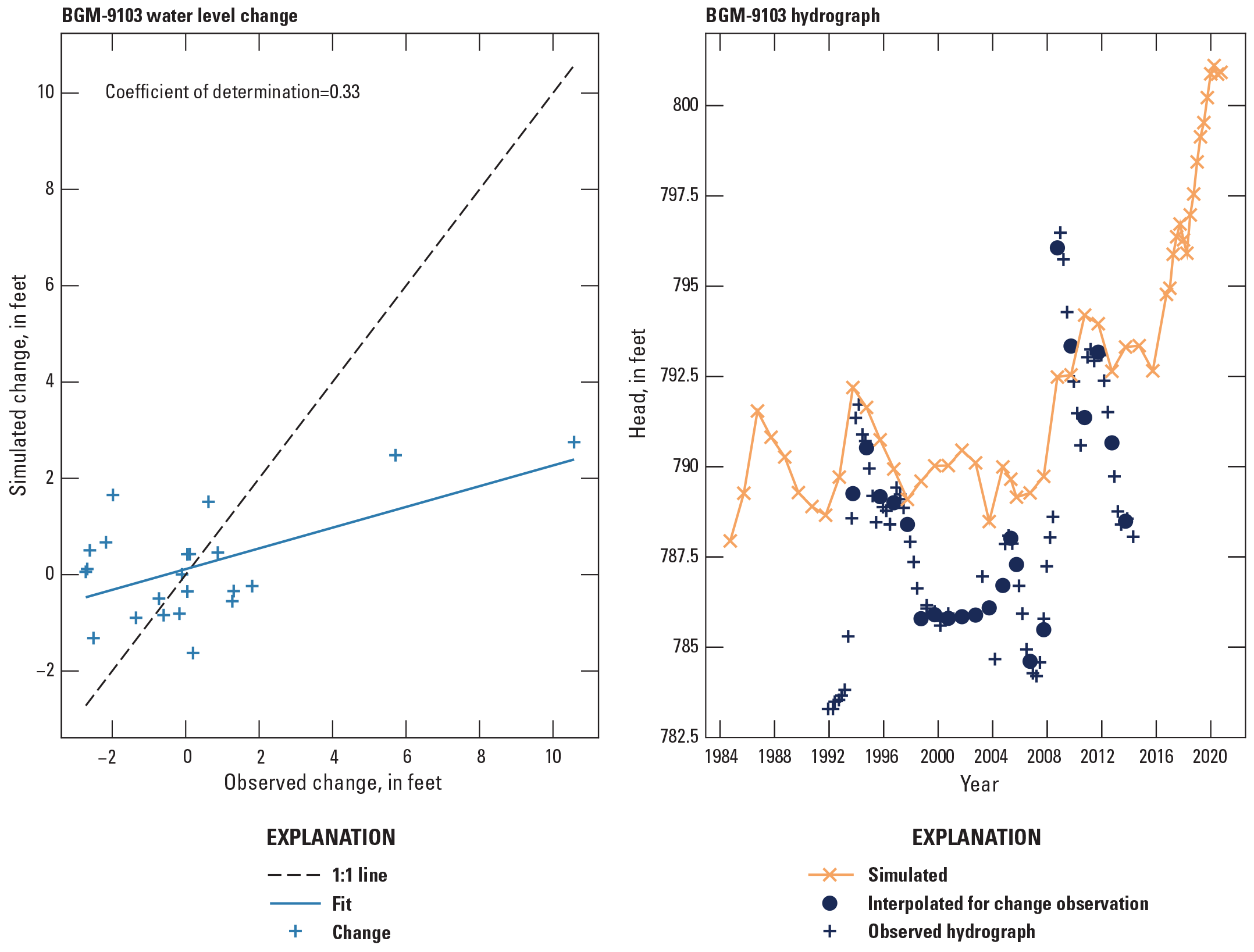
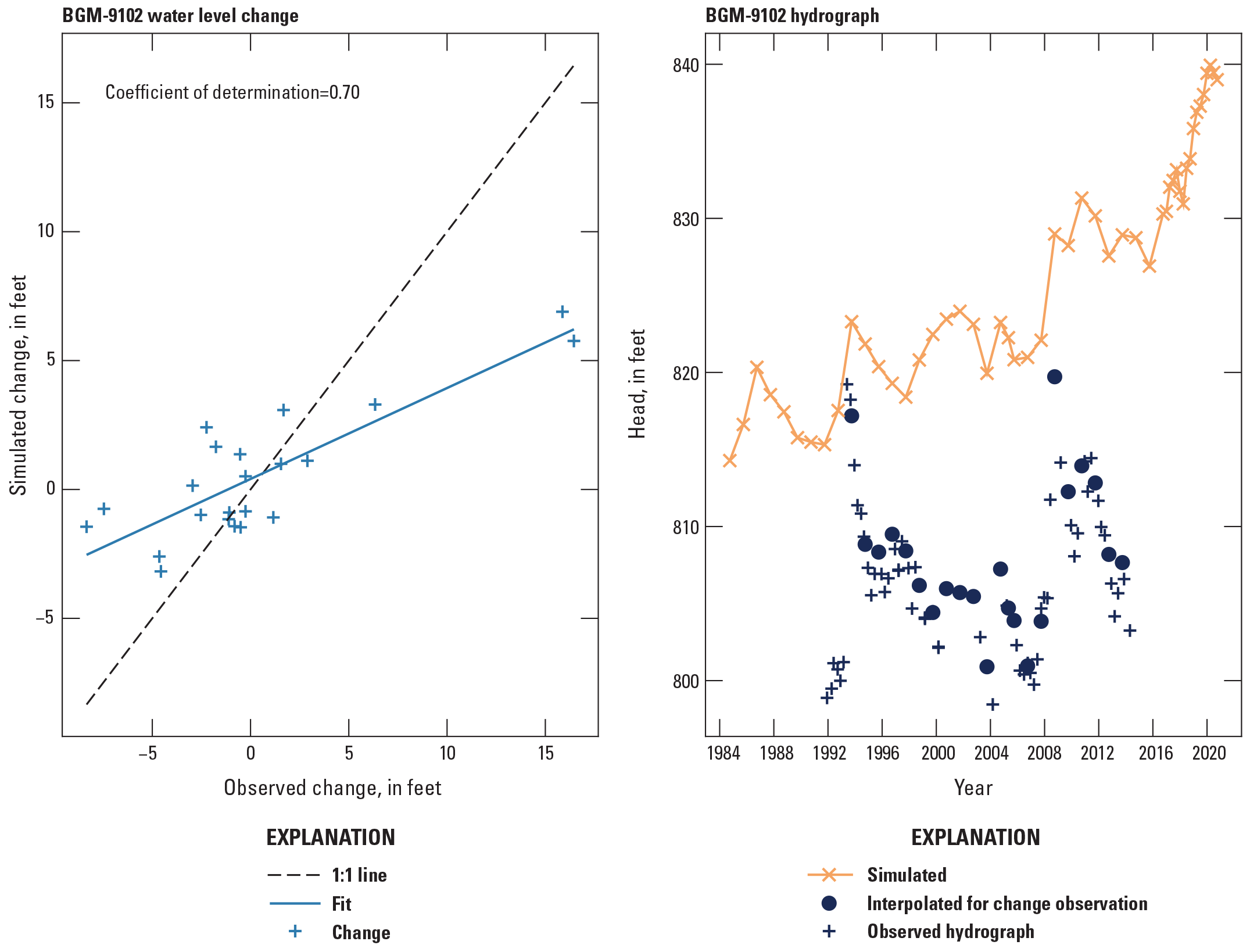
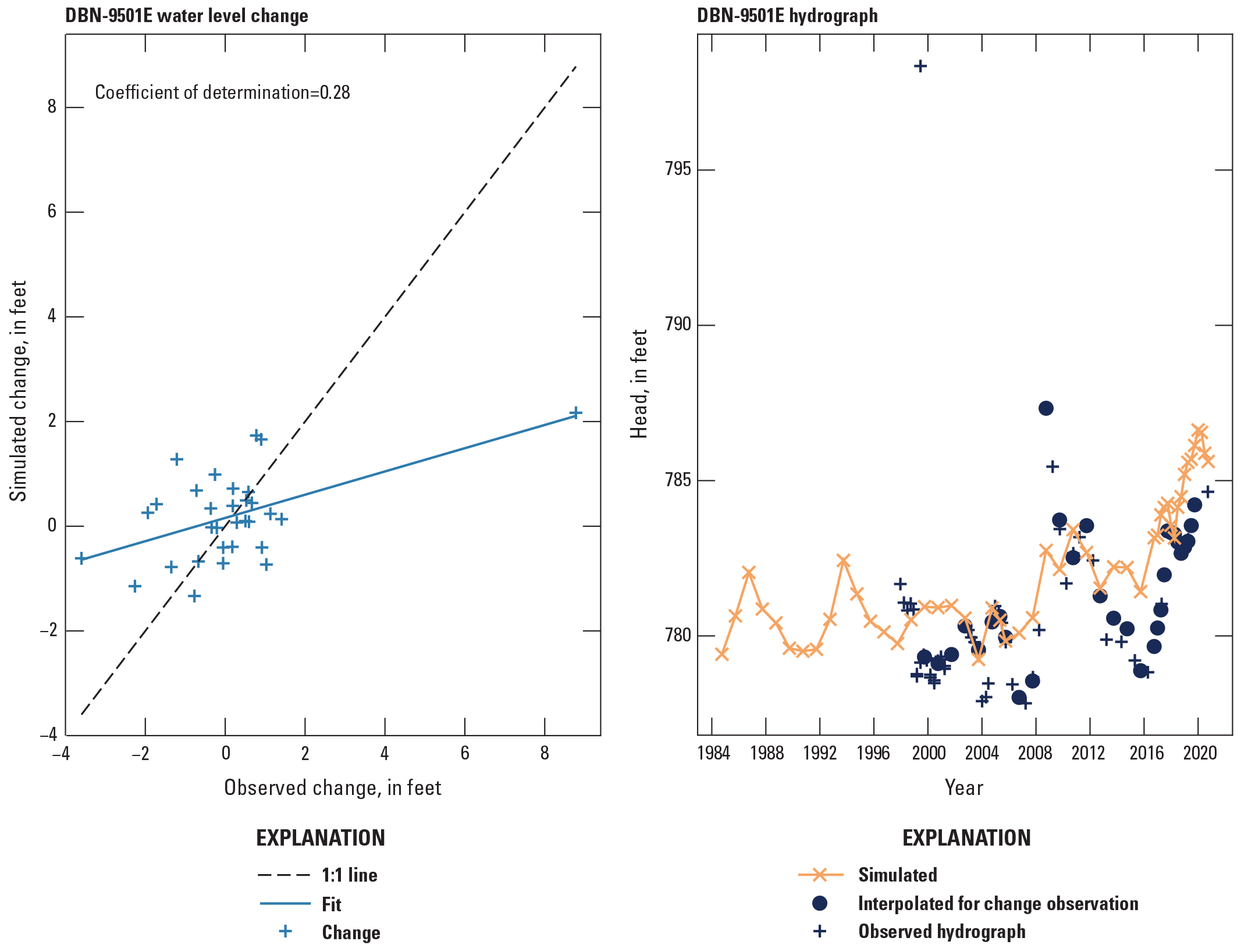
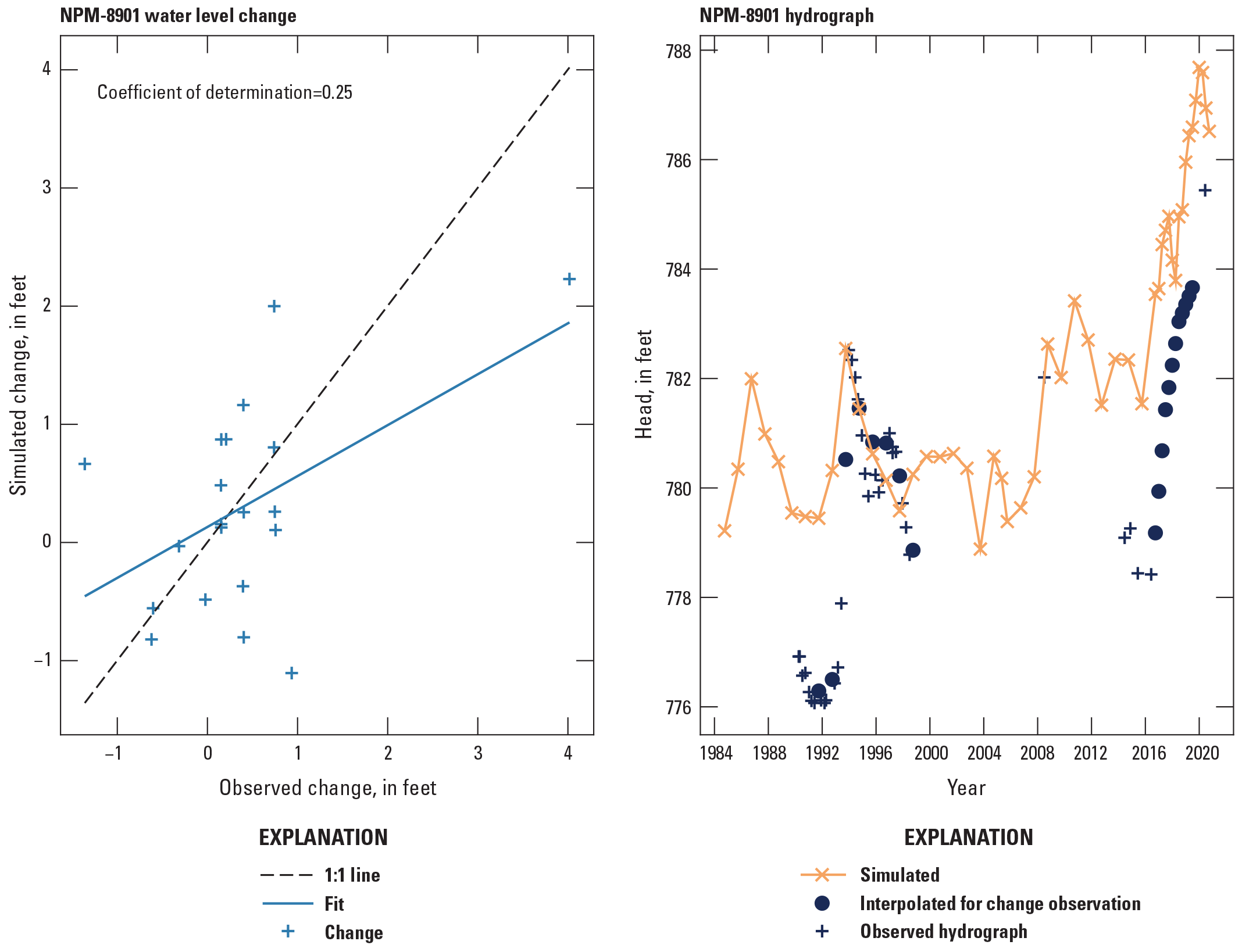
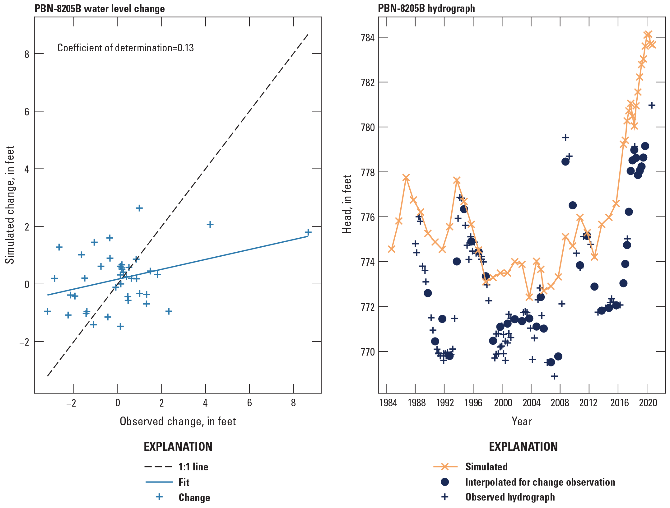
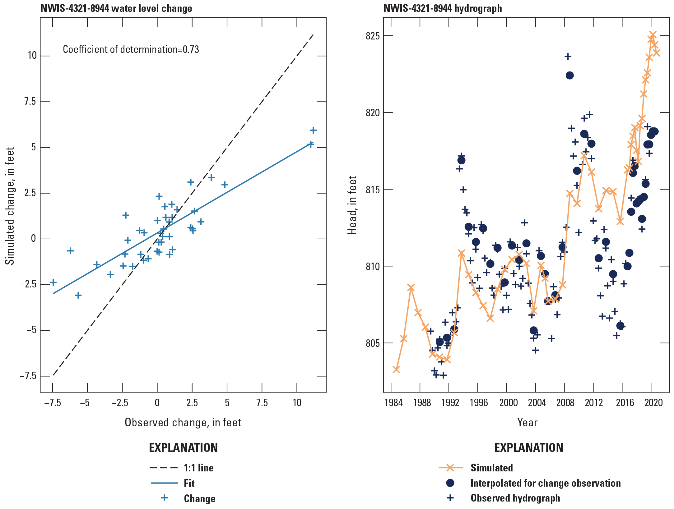
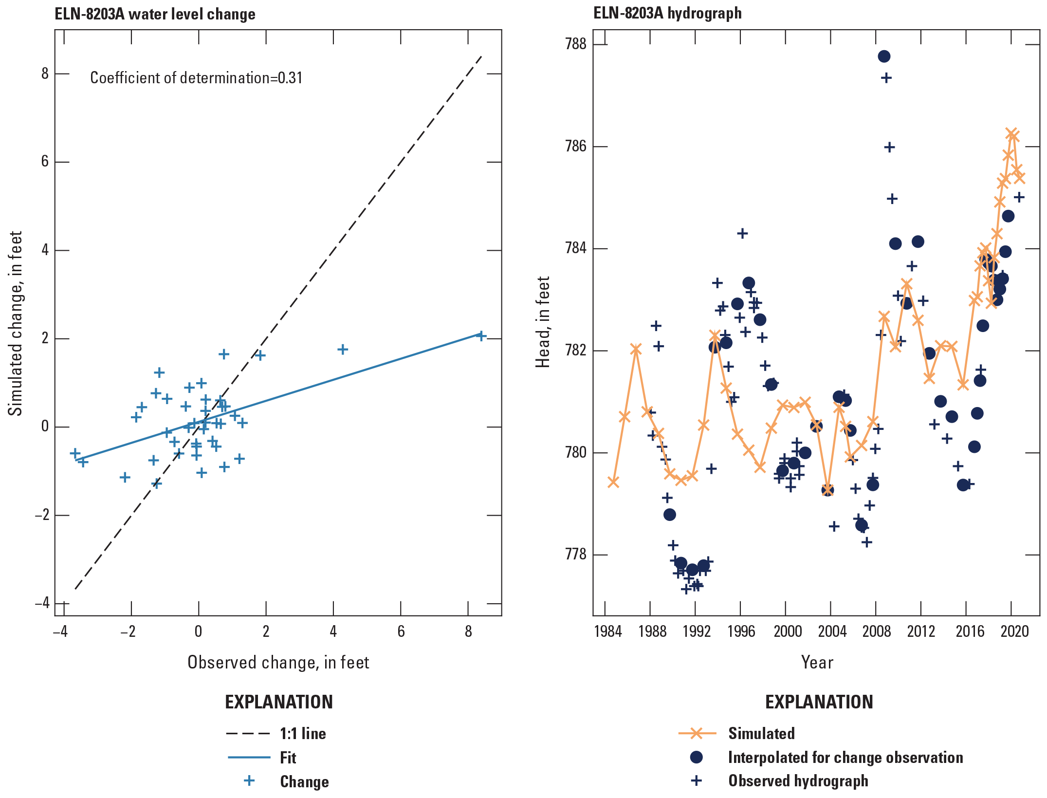
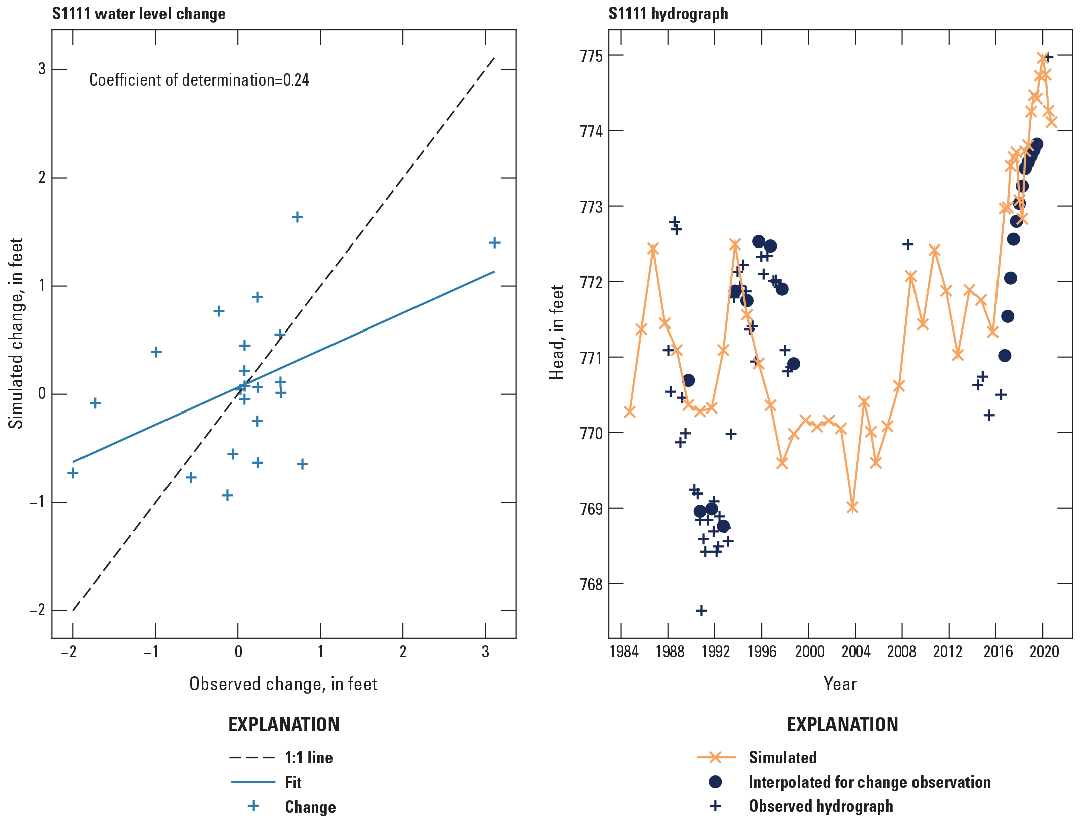
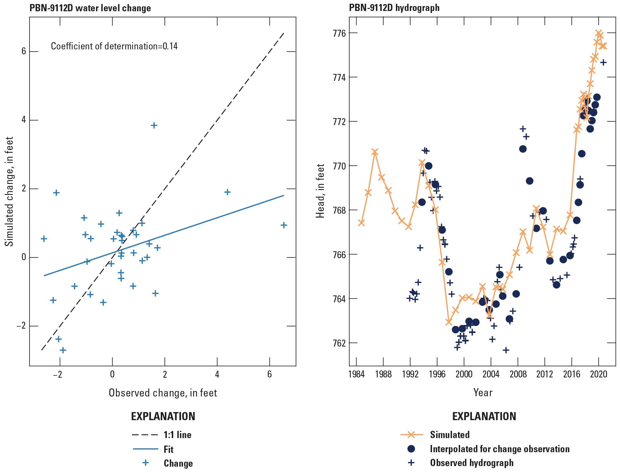
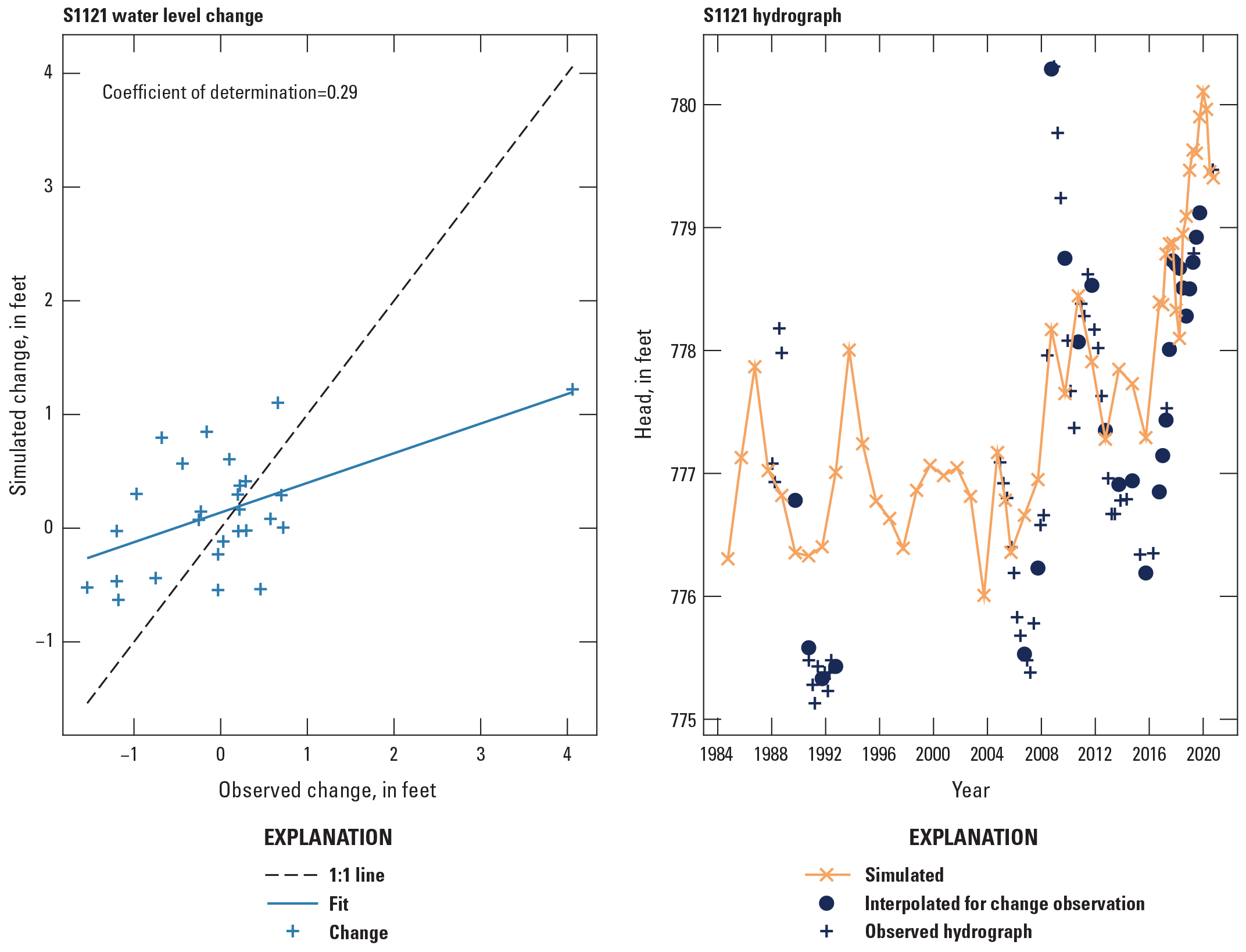

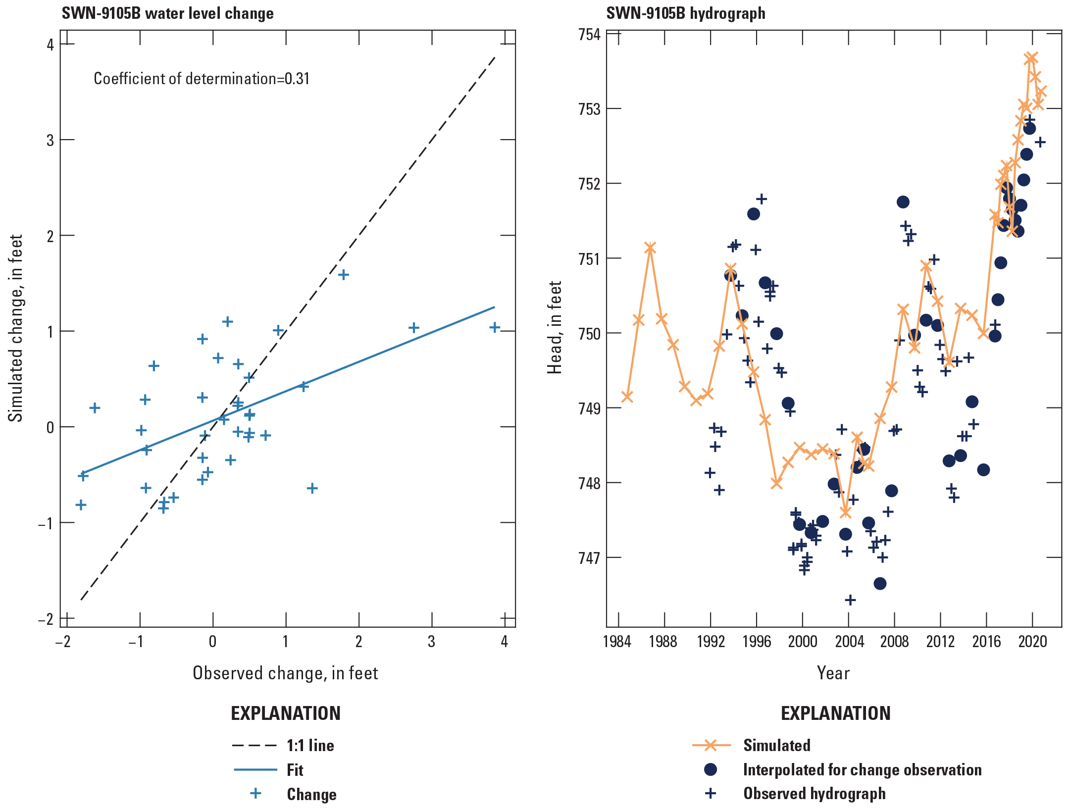
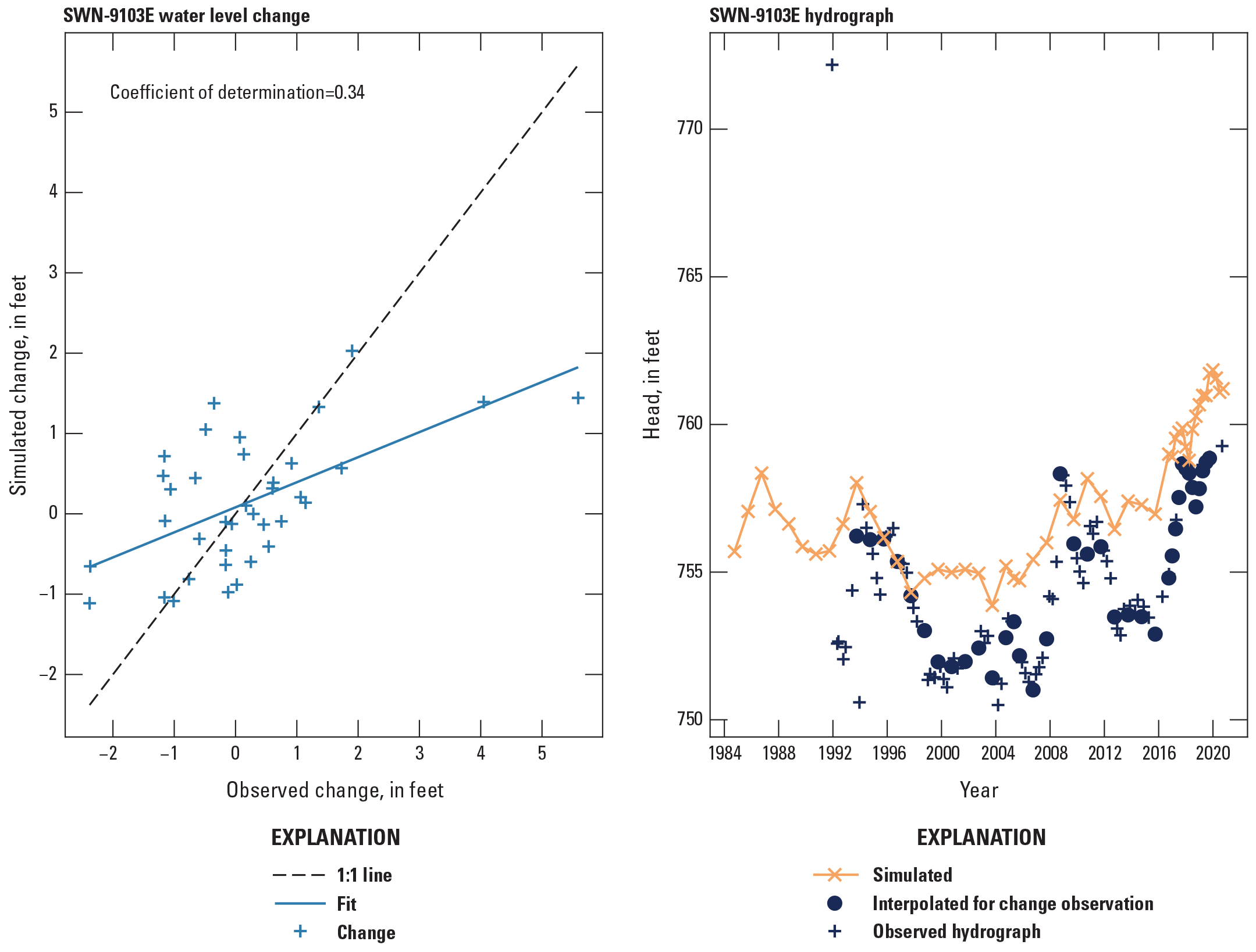
Observed and simulated change in water level and hydrograph for wells in the set 3 timeseries hydrographs.
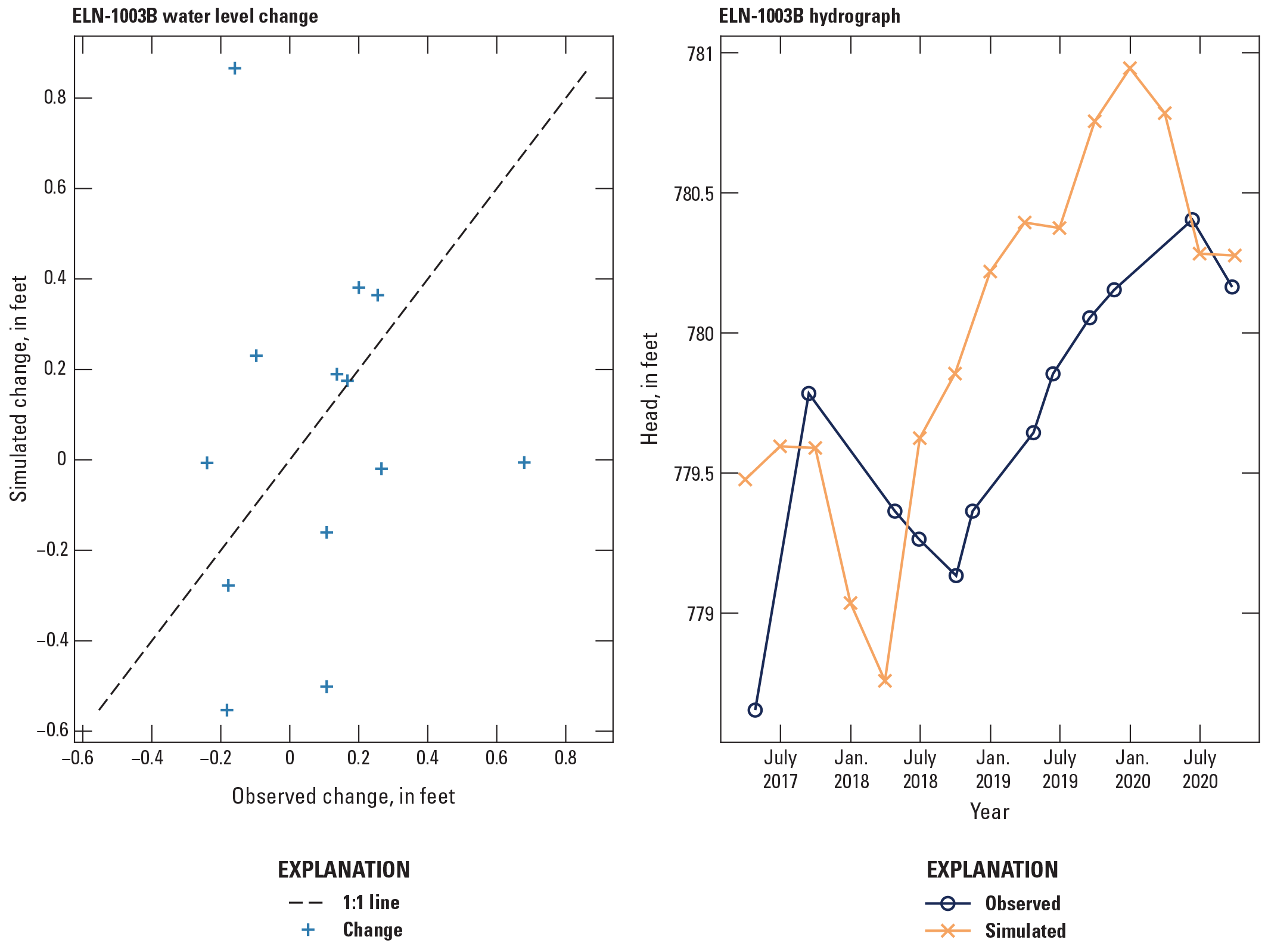
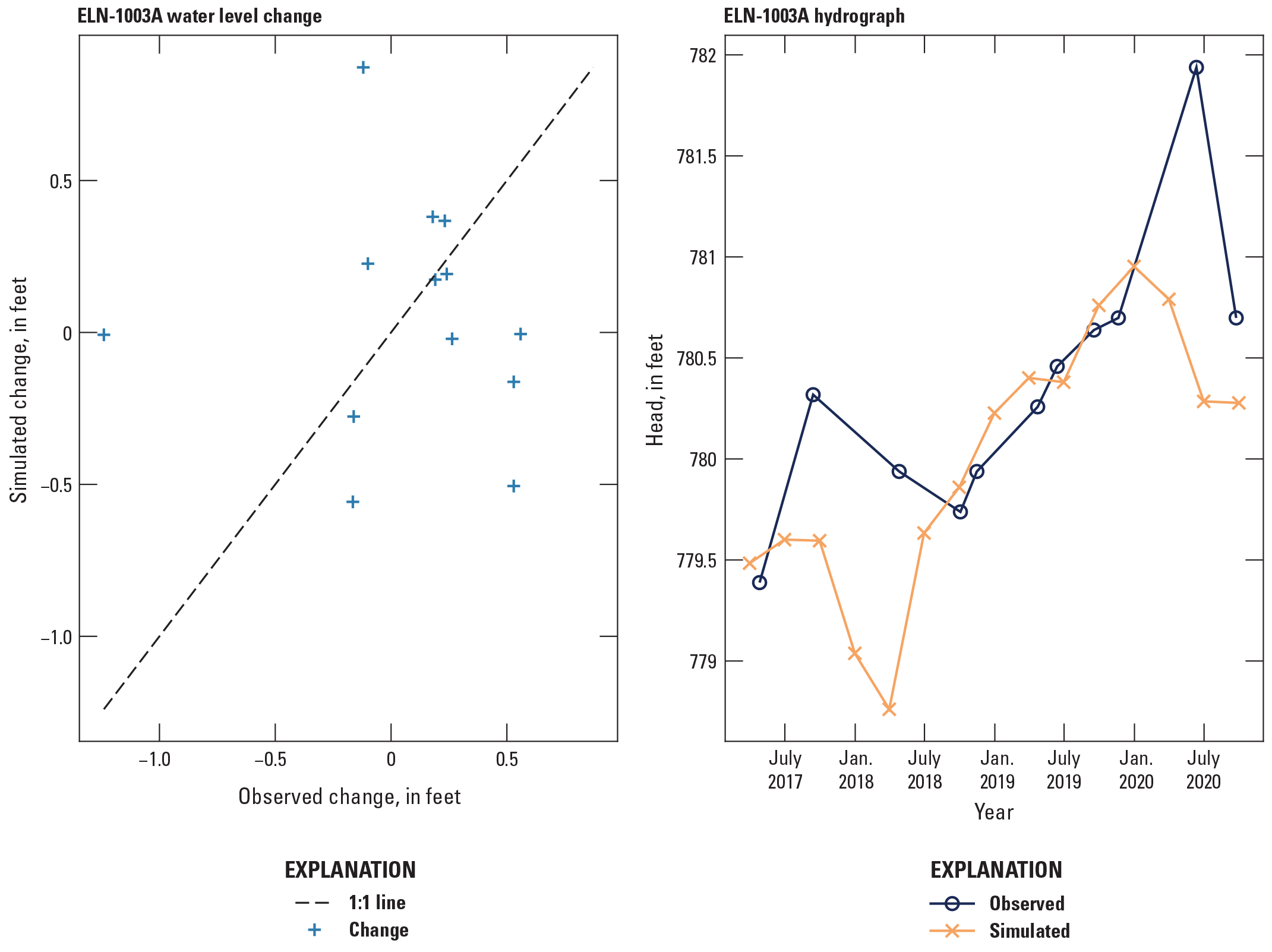
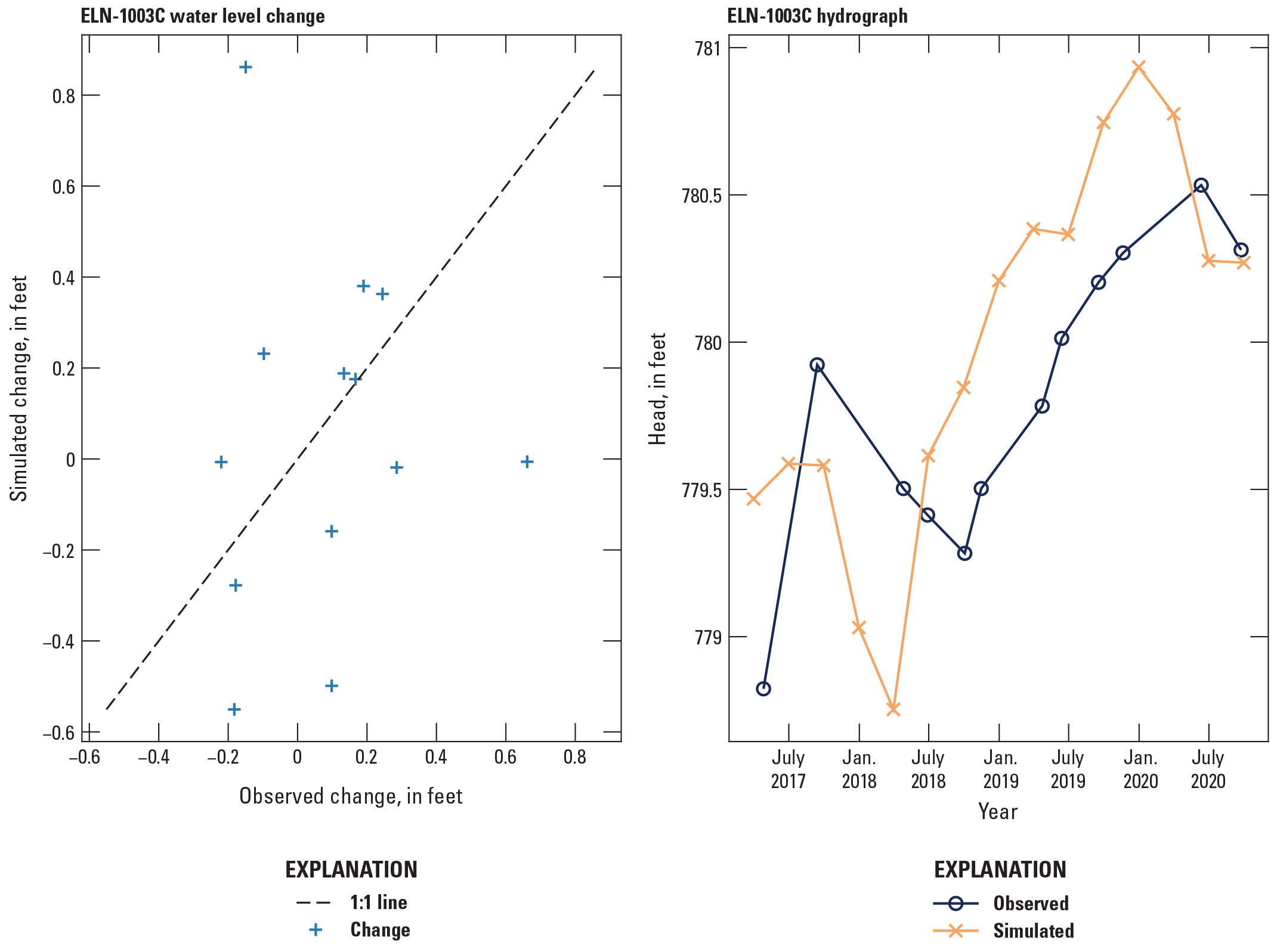
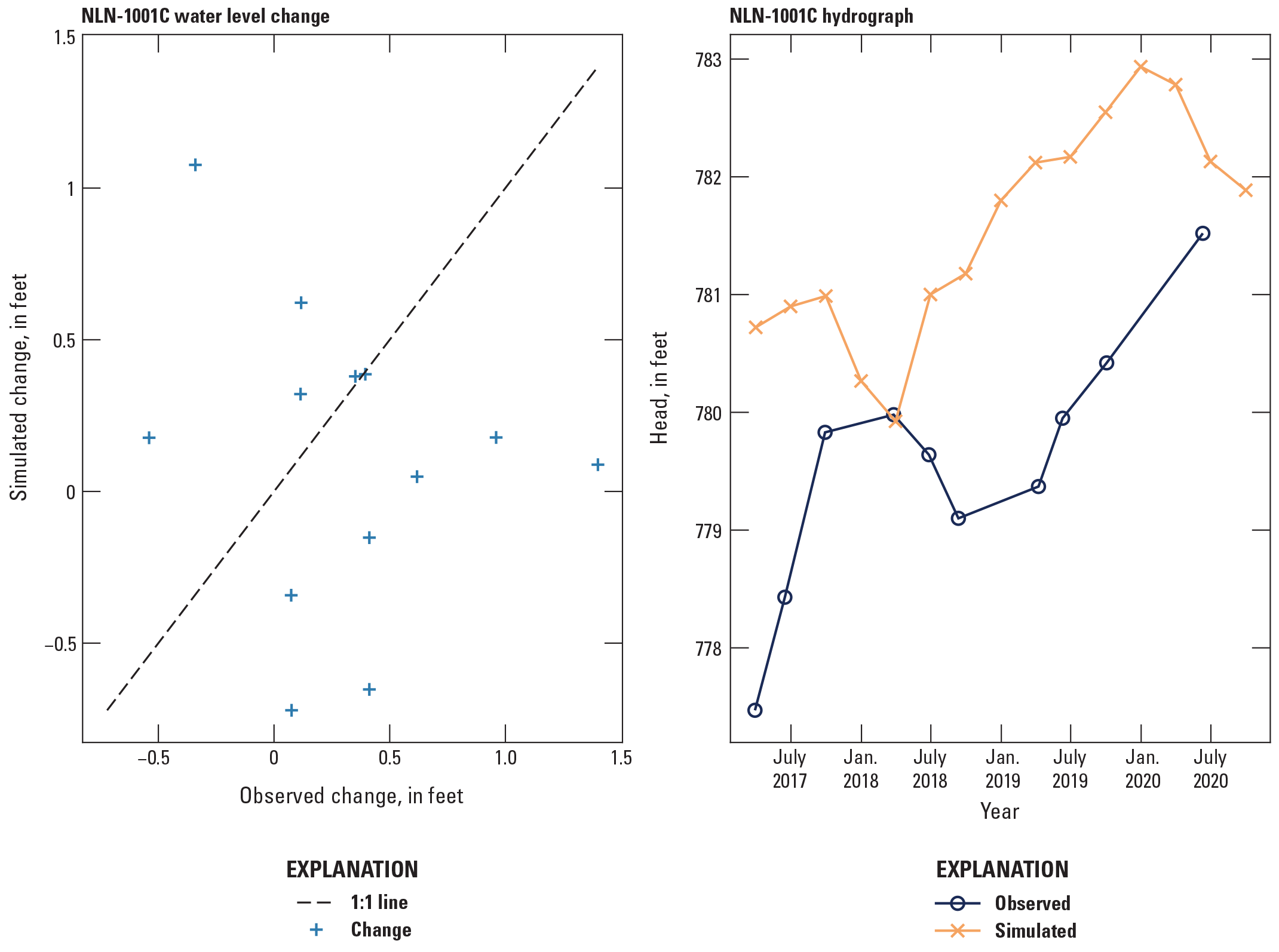
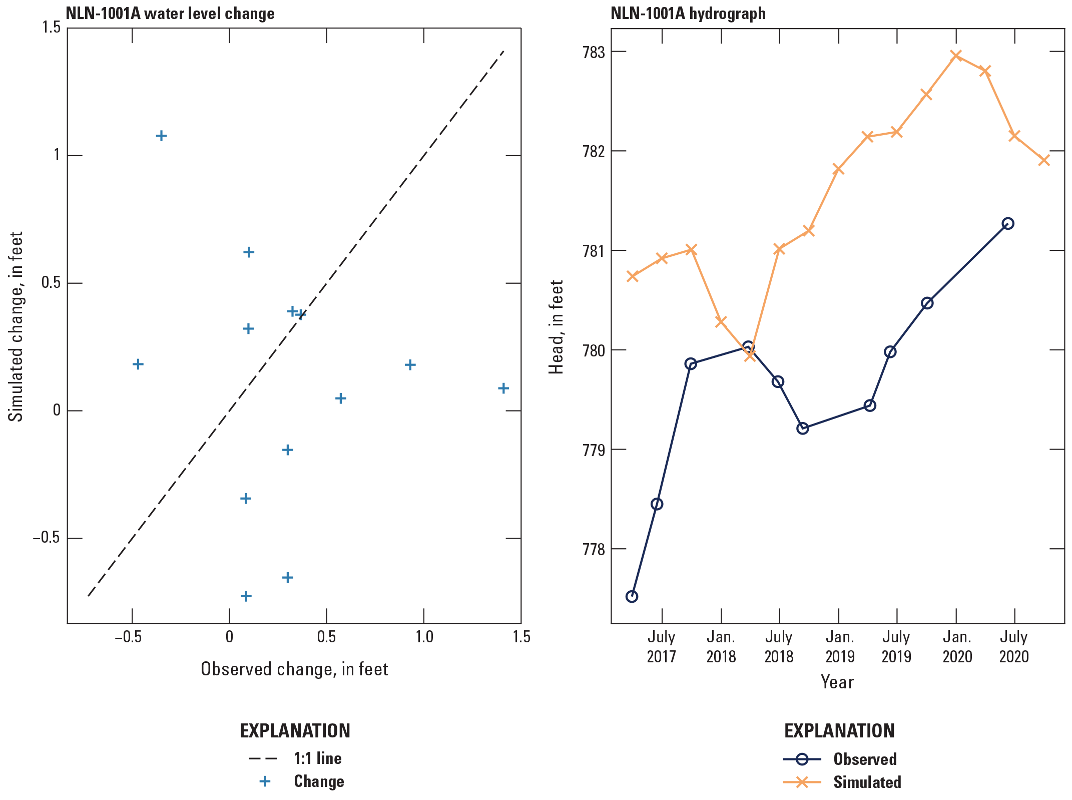
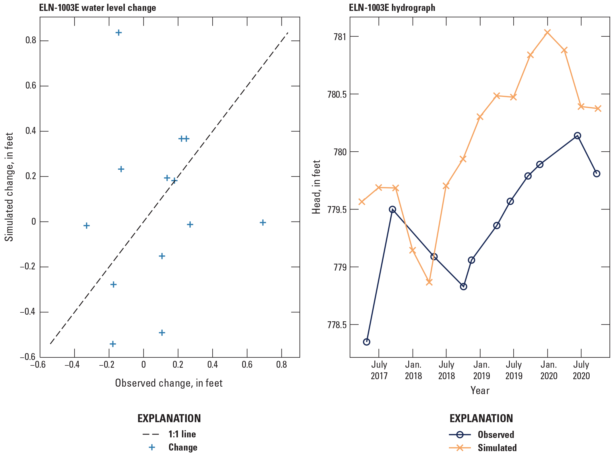
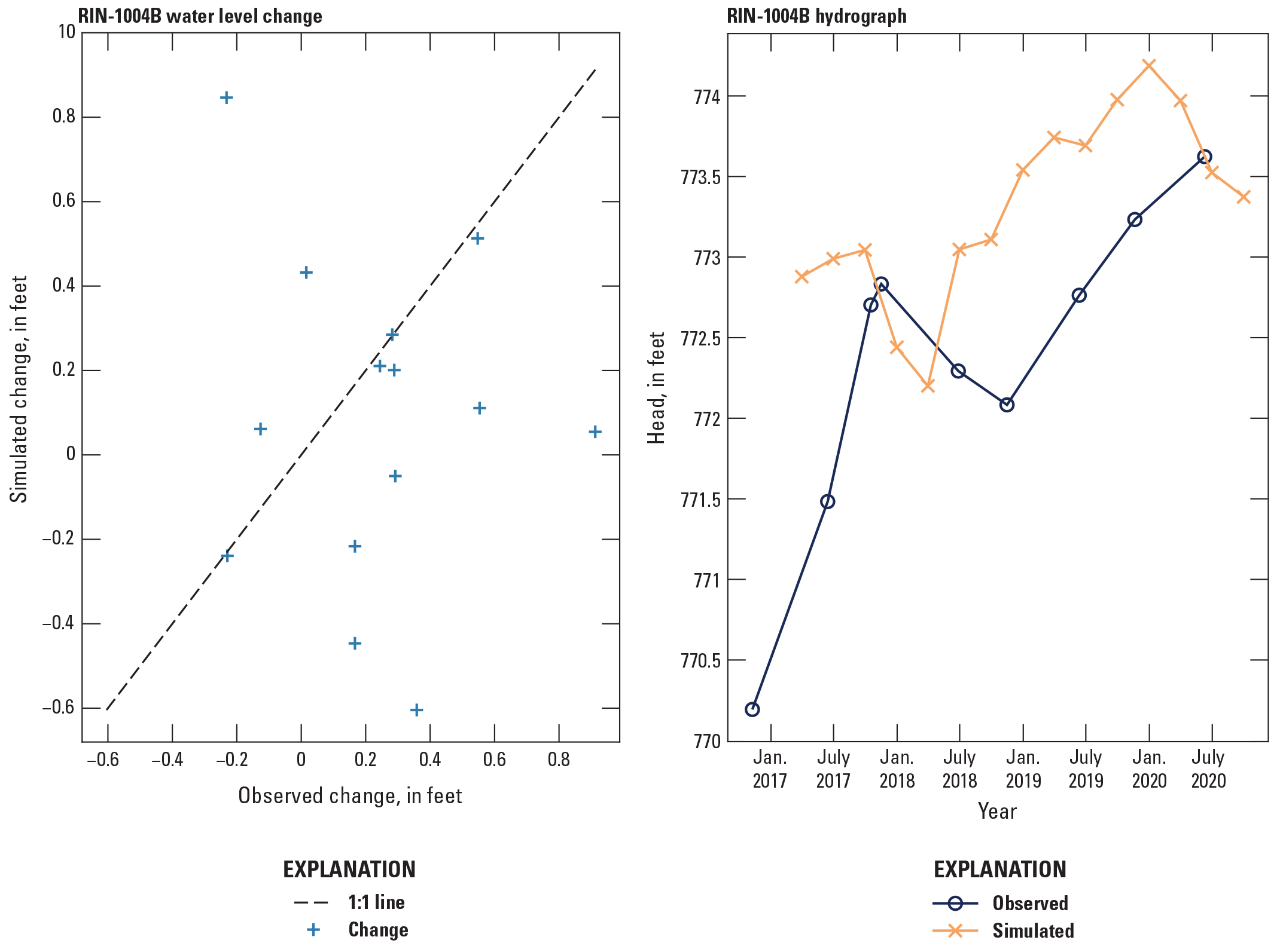
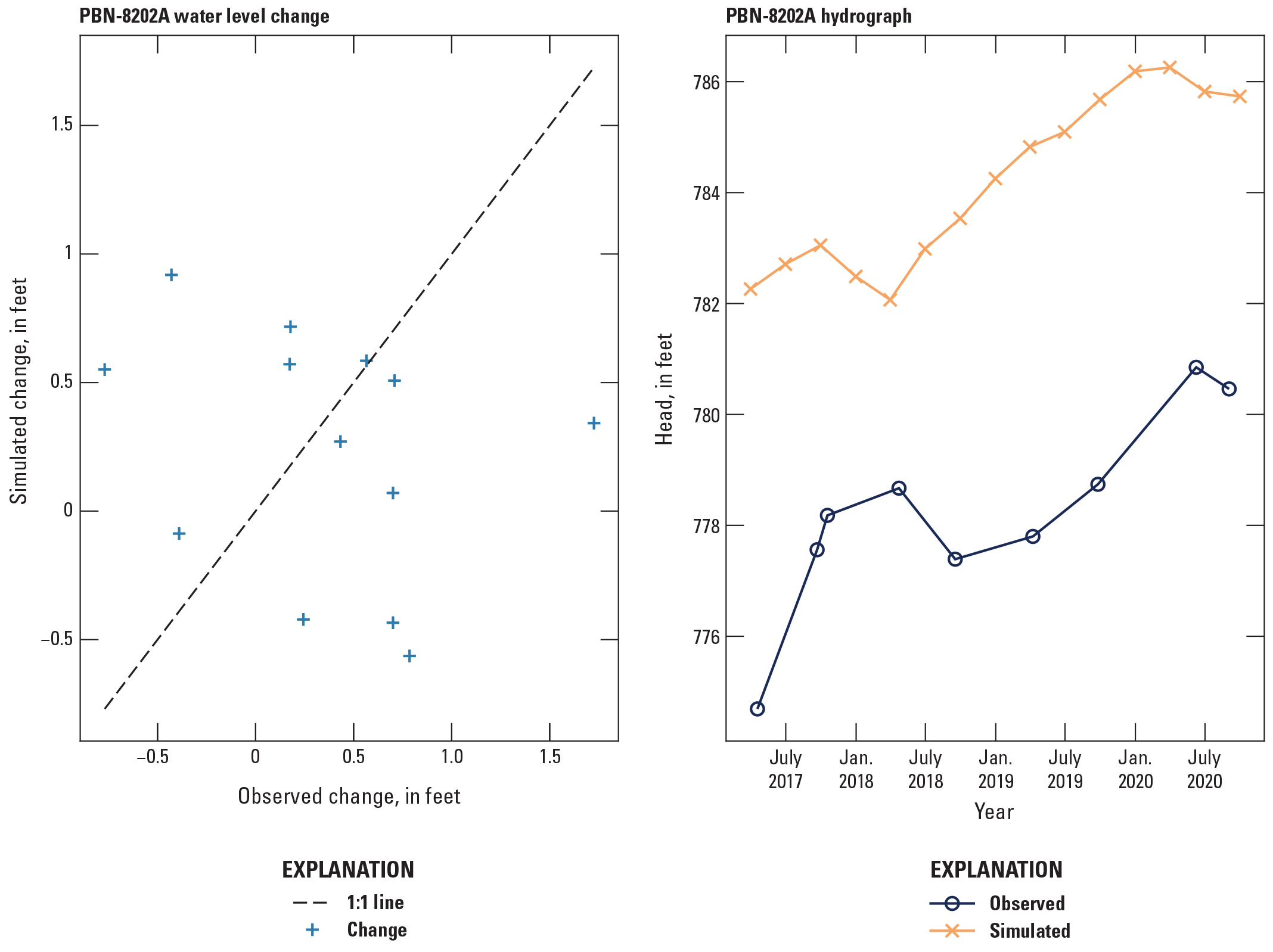
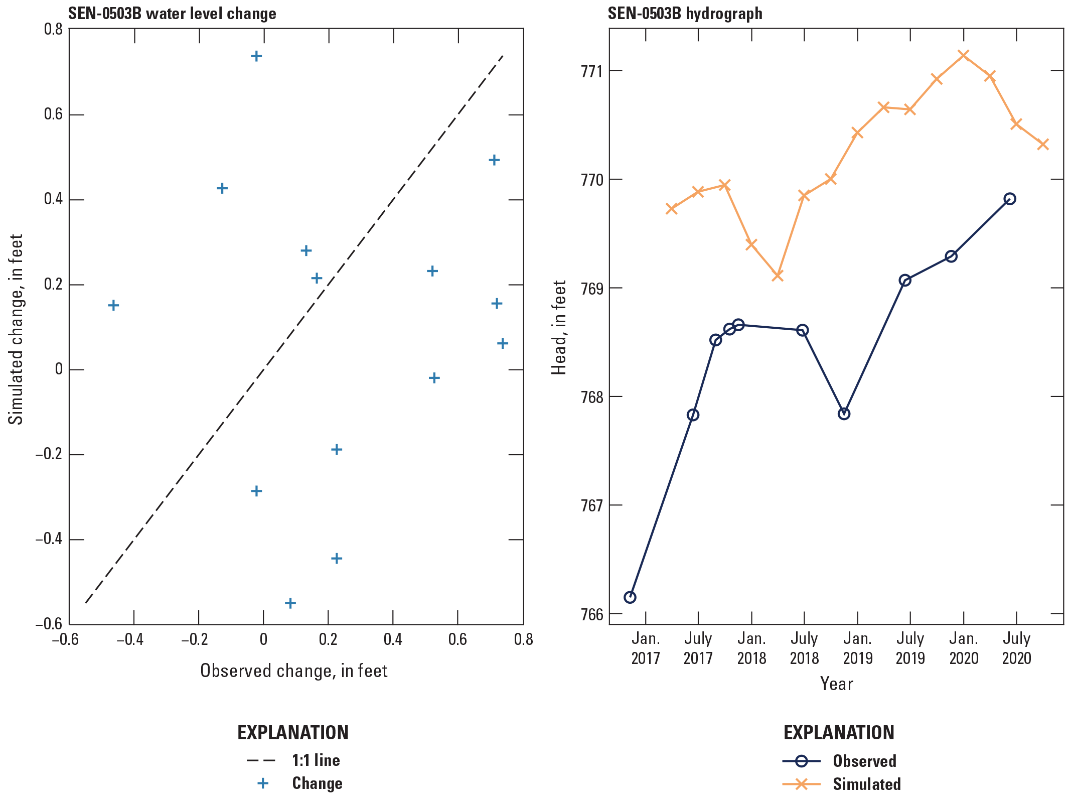
Observed and simulated change in water level and hydrograph for wells in the set 4 seasonal timeseries hydrographs.
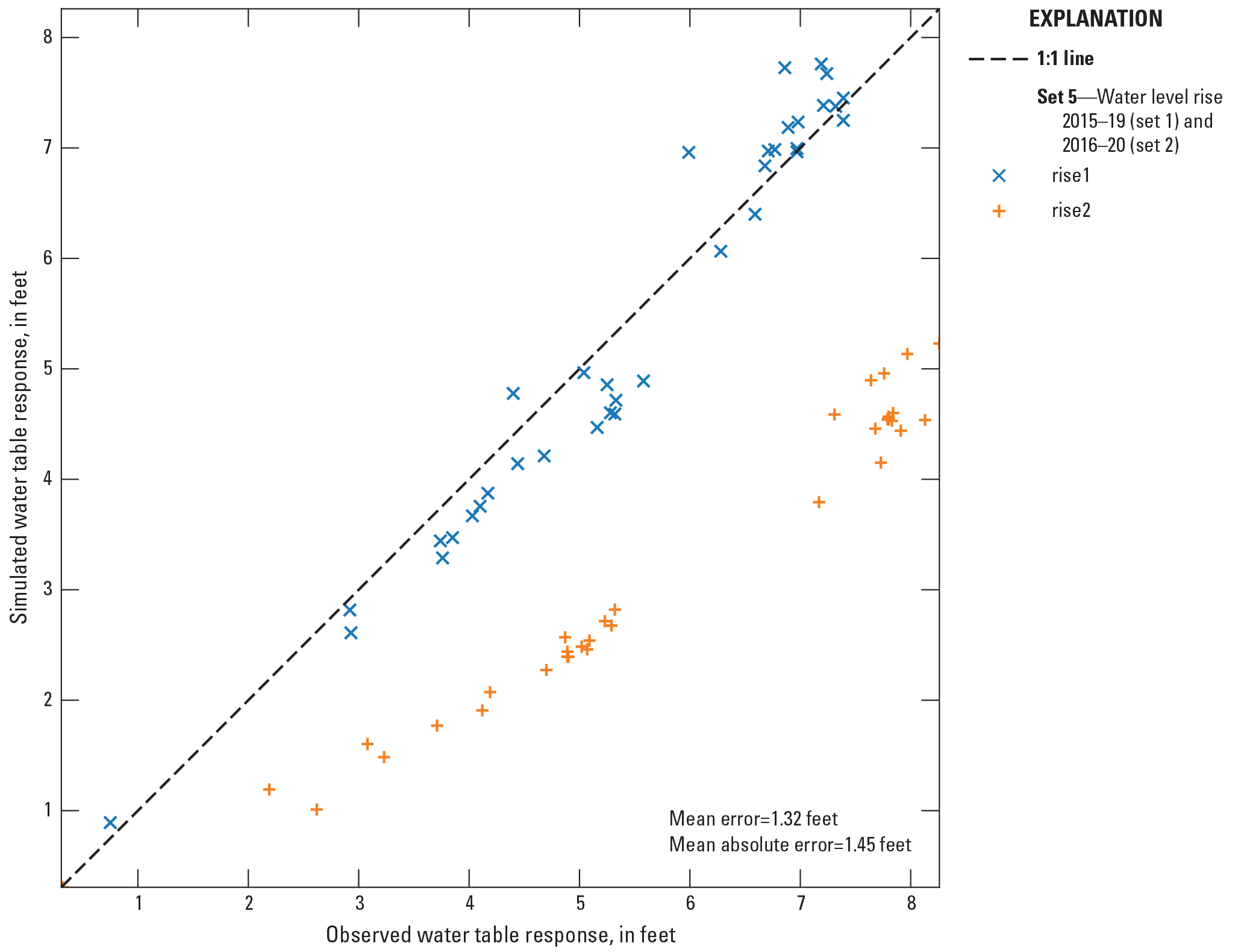
Observed and simulated water table response for the two periods (rise 1 and rise 2) in the set 5 water level rise observation group using the base model.
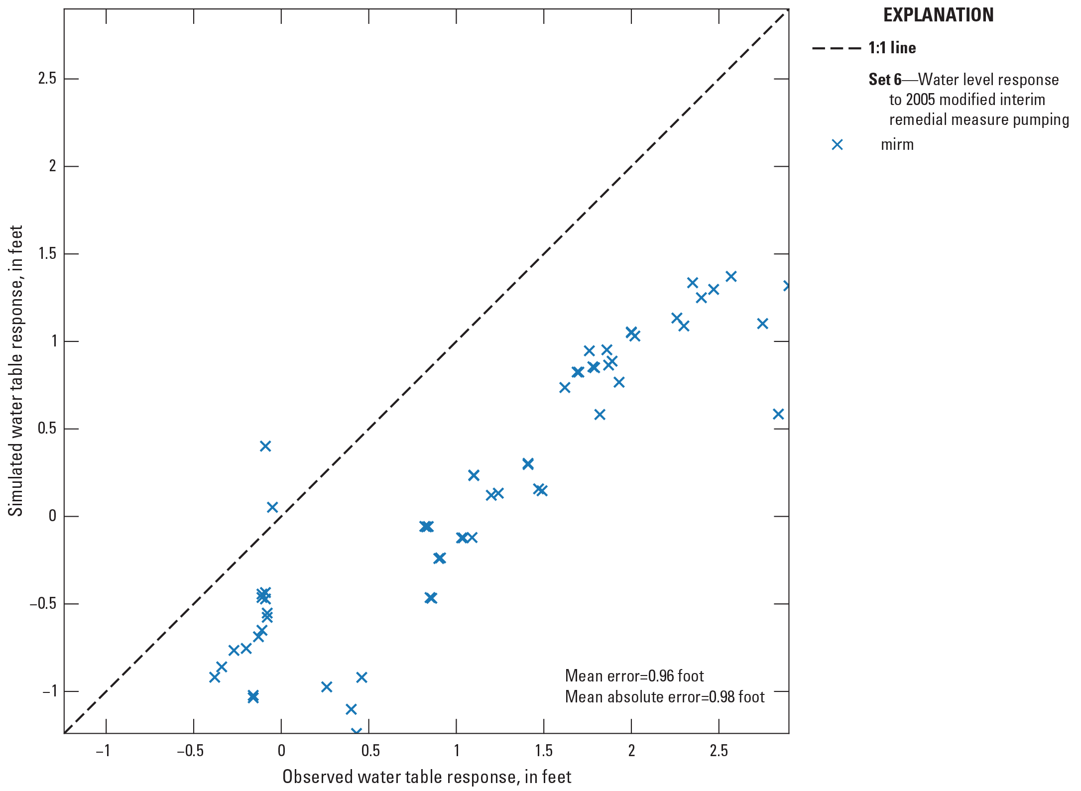
Observed and simulated water table response to the MIRM pumping in the set 6 (MIRM) observation group using the base model.
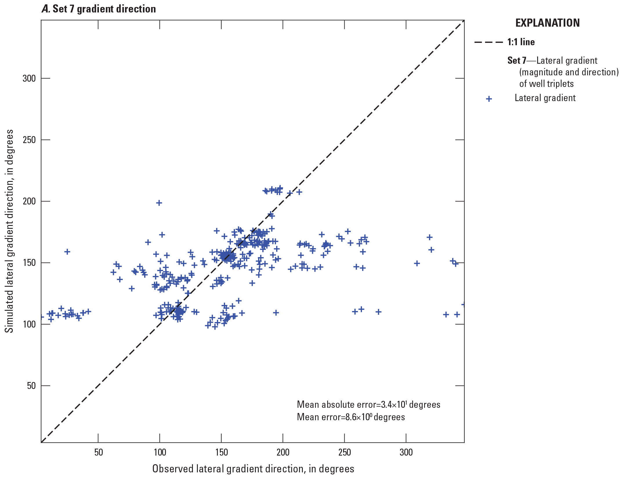
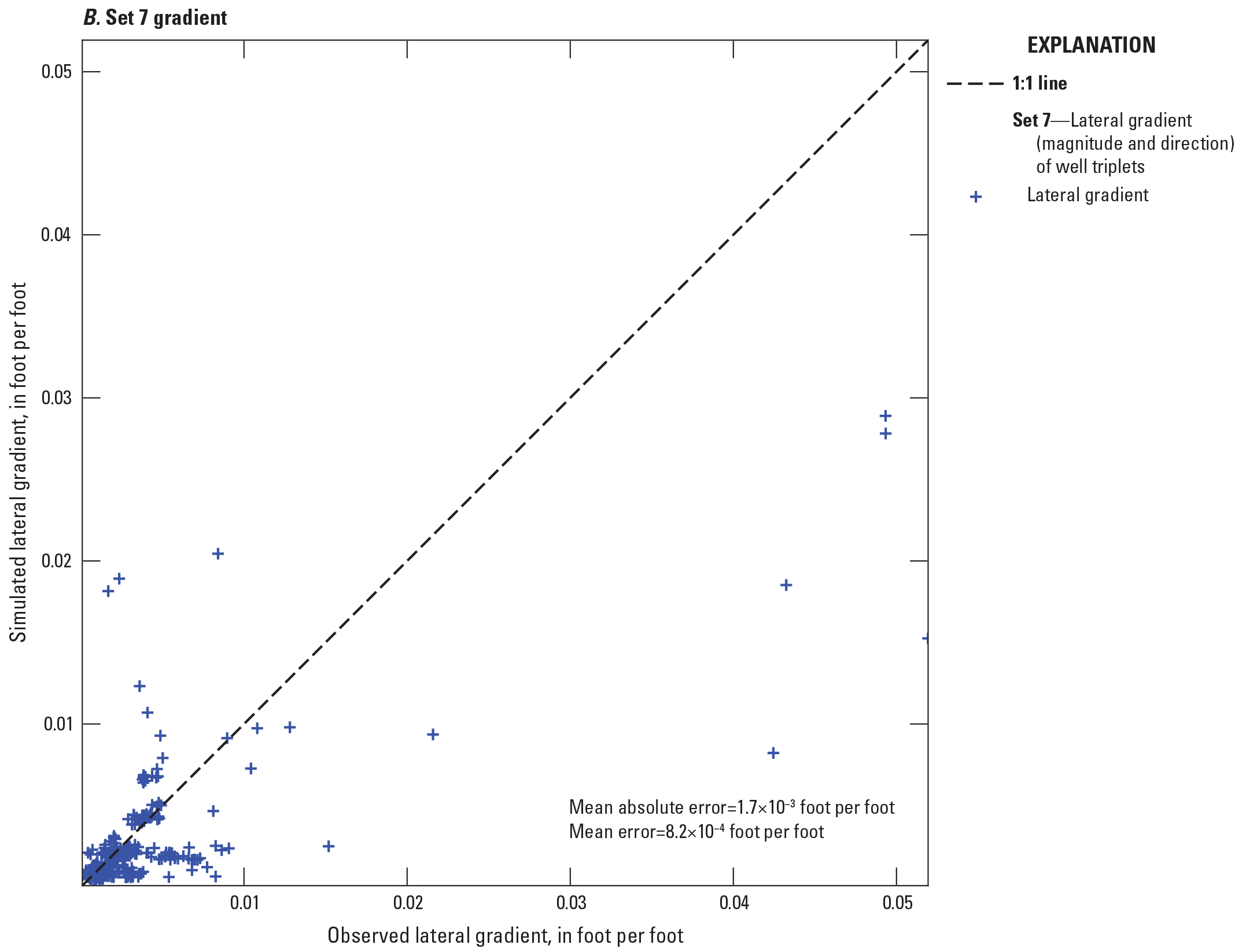
Observed and simulated lateral gradient direction and magnitude in the set 7 lateral gradient observation group using the base model.
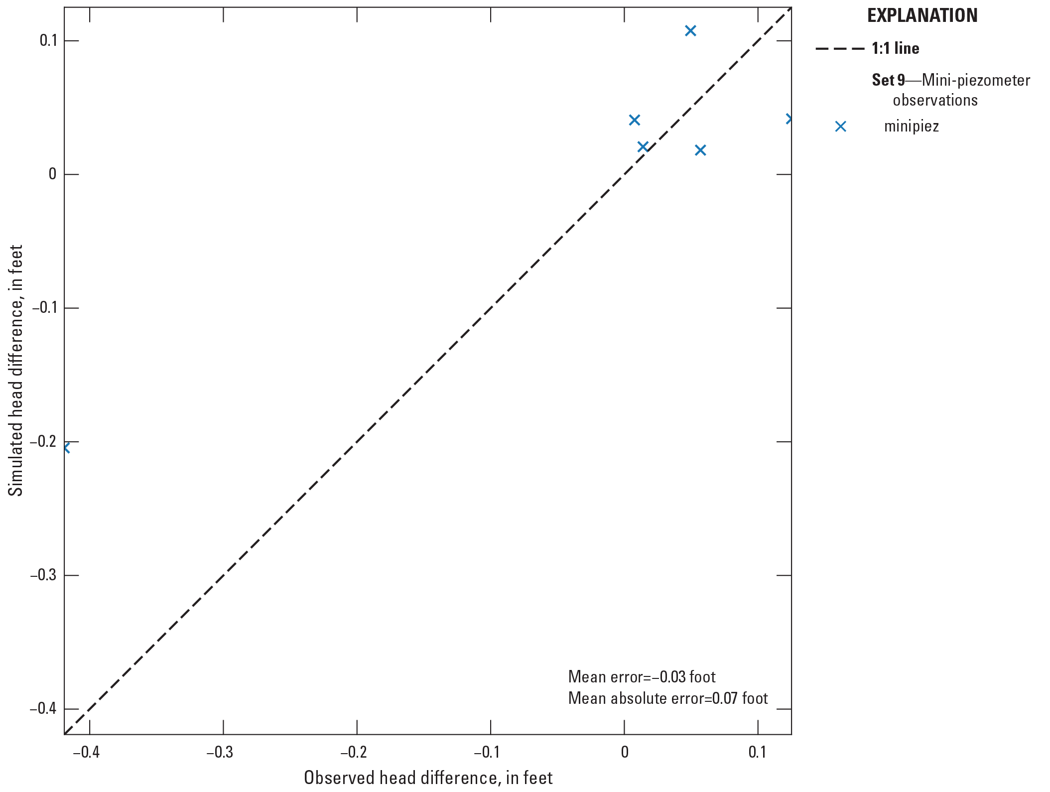
Observed and simulated hydraulic head differences between the mini-piezometer water level and the Wisconsin River stage in the set 9 (minipiez) observation group using the base model.
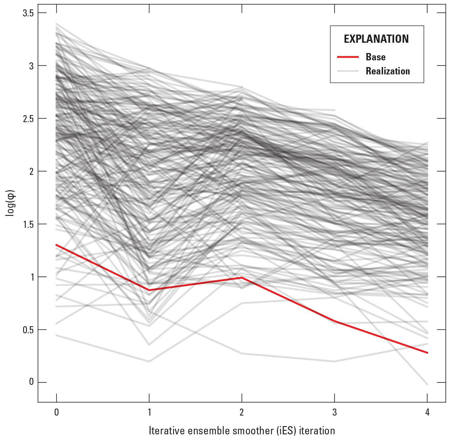
Graph of phi over time for assessing paths of the set 10 MODPATH plume particles originating in the plume source area relative to the plume outline.
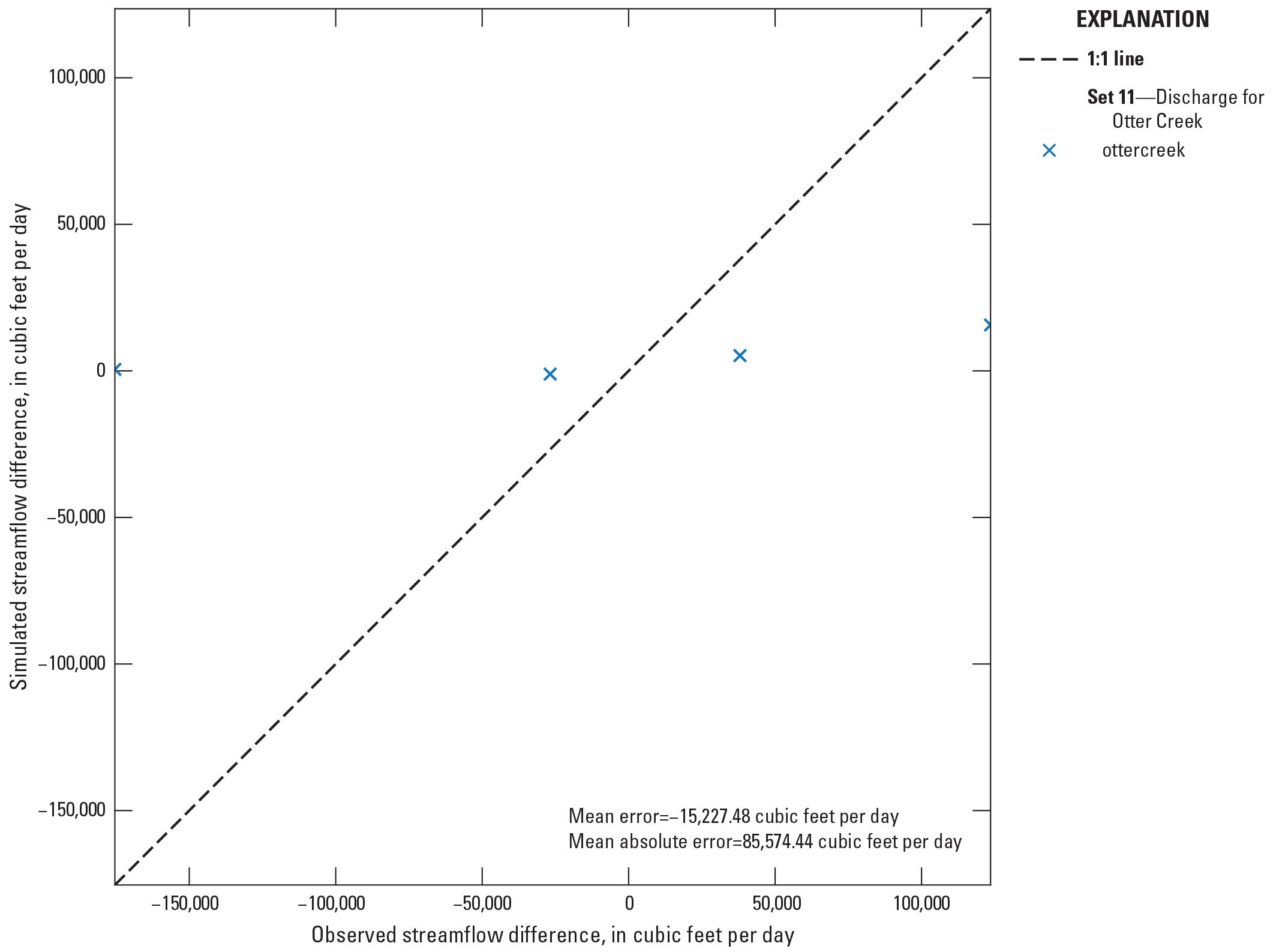
Observed and simulated streamflow differences in Otter Creek in the set 11 (ottercreek) observation group using the base model.
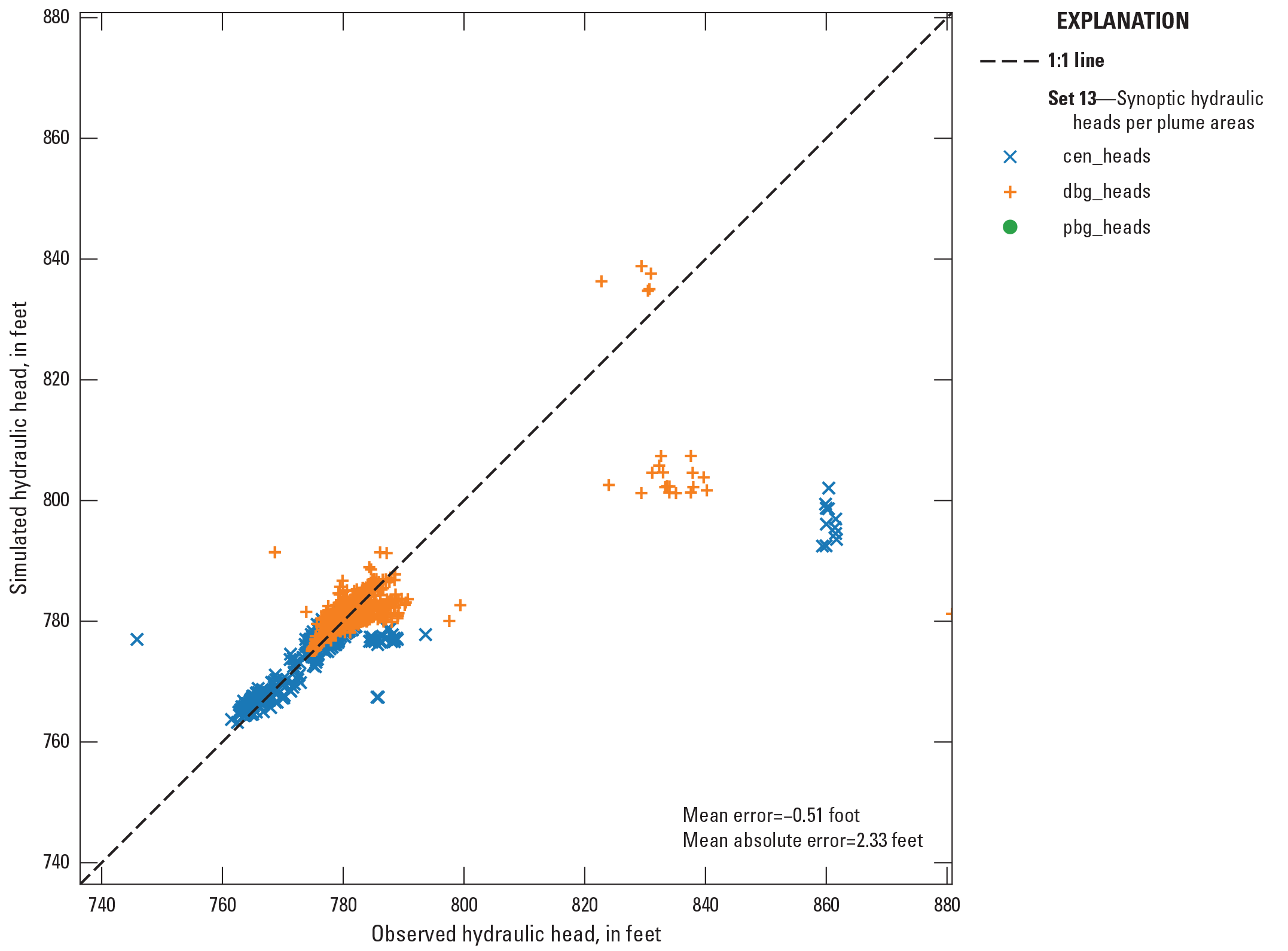
Observed and simulated synoptic hydraulic heads in the plume areas for the set 13 (pbg_heads, dbg_heads, cen_heads) observation group using the base model.
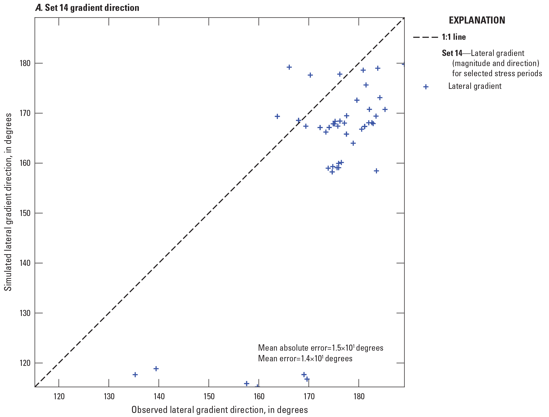
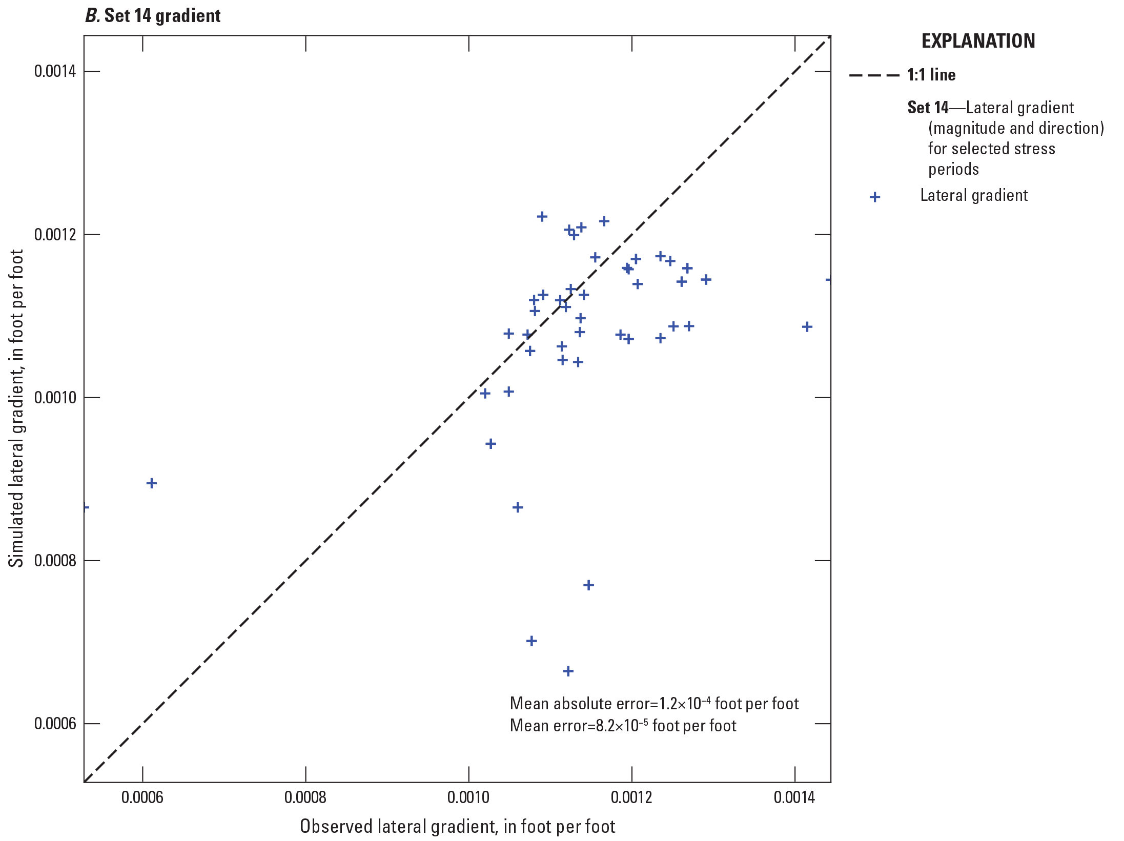
Observed and simulated lateral gradient direction and magnitude in the set 14 gradient observation group using the base model.
A Method of Morris sensitivity analysis was performed using the PESTPP–SEN module to assess the sensitivity of the model calibration parameters to each observation. The top 50 most sensitive combinations are plotted in log space in figure 4.19. Of these, the top 5 correspond to the plume polygons. This suggests that the model calibration was sensitive to the plume footprints and should push the calibration towards a model that can robustly simulate flow in the plume areas. This is particularly important given the model goal of providing a reasonable advective component for the groundwater transport model.
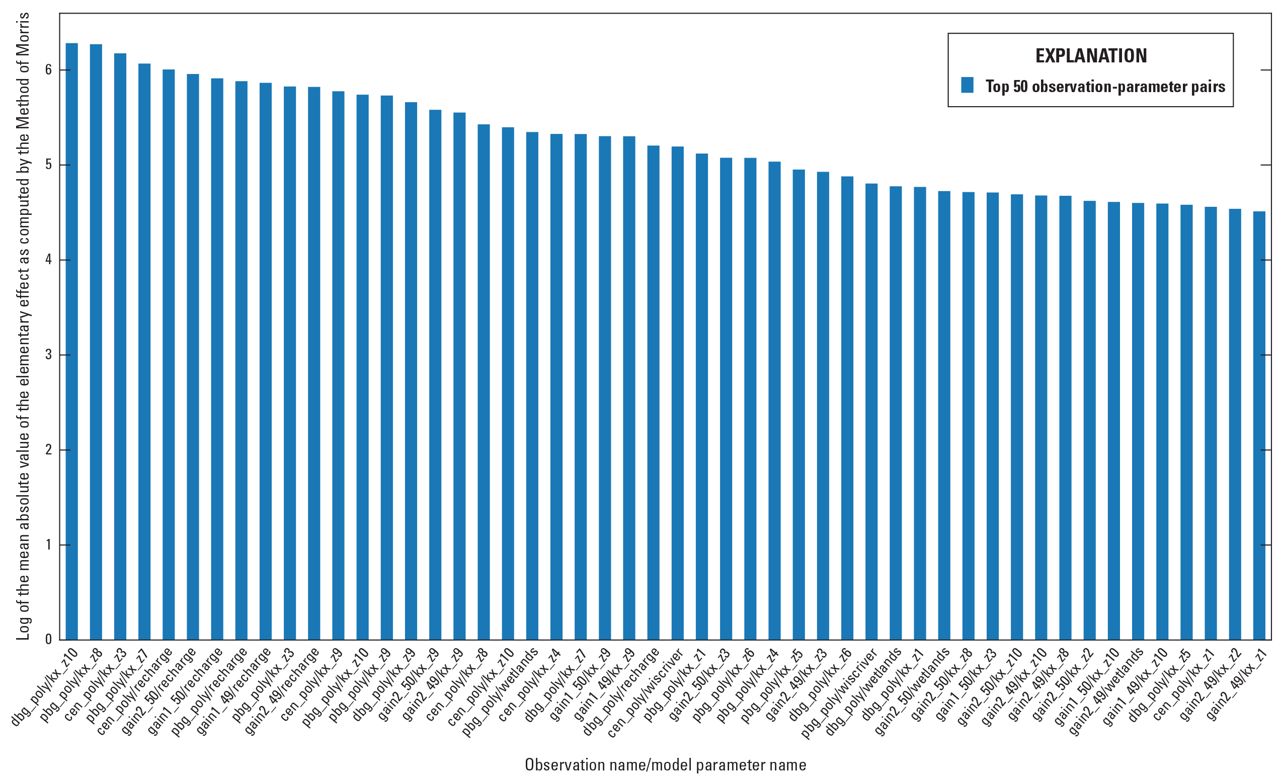
Method of Morris sensitivity results.
References Cited
Pollock, D.W., 2016, User guide for MODPATH version 7—A particle-tracking model for MODFLOW: U.S. Geological Survey Open-File Report 2016–1086, 35 p., accessed September 2022 at https://doi.org/10.3133/ofr20161086.
Ruskauff, G.J., and Rumbaugh, J.O., Jr., 1996, Incorporating groundwater flow direction and gradient into a flow model calibration, in Kovar, K., and van. der, P., eds., Calibration and reliability in groundwater modelling [Proceedings of the ModelCARE‘96 conference held at Golden, Colorado, September 24–26, 1996]: IAHS Press, p. 71–81, accessed September 2022 at https://agris.fao.org/agris-search/search.do?recordID=GB9705120.
SpecPro Professional Services, LLC, 2019, Remedial investigation/feasibility study for site-wide groundwater at the former Badger Army Ammunition Plant, Baraboo, Wisconsin: SpecPro Professional Services, LLC, 717 p., accessed March 2020 at https://cswab.org/wp-content/uploads/2020/05/Badger-Army-Site-Wide-Groundwater-RIFS-Study-DRAFT-Nov-2019.pdf.
U.S. Geological Survey, 2021, USGS water data for the Nation: U.S. Geological Survey National Water Information System database, accessed September 2021 at https://doi.org/10.5066/F7P55KJN.
Westenbroek, S.M., Doherty, J., Walker, J.F., Kelson, V.A., Hunt, R.J., and Cera, T.B., 2012, Approaches in highly parameterized inversion—TSPROC, a general time-series processor to assist in model calibration and result summarization: U.S. Geological Survey Techniques and Methods, book 7, chap. C7, 79 p., accessed September 2022 at https://pubs.usgs.gov/tm/tm7c7/pdf/TM7_C7_112712.pdf.
Conversion Factors
U.S. customary units to International System of Units
Temperature in degrees Fahrenheit (°F) may be converted to degrees Celsius (°C) as follows: °C = (°F – 32) / 1.8.
Datum
Vertical coordinate information is referenced to the North American Vertical Datum of 1988 (NAVD 88).
Elevation, as used in this report, refers to distance above the vertical datum.
Abbreviations
BAAP
Badger Army Ammunition Plant
DBG
deterrent burning ground
DNT
dinitrotoluene
DRN
drain package
iES
iterative ensemble smoother
IRM
interim remedial measure
KGS
Kansas Geological Survey
Kh
horizontal hydraulic conductivity
Kv
vertical hydraulic conductivity
MIRM
modified interim remedial measure
MNW2
multinode well package
MODFLOW–NWT
transient groundwater flow model using the Newton Raphson formulation
NC
nitrocellulose
NWIS
National Water Information System
PBG
propellant burning ground
RIV
river package
SFR2
streamflow-routing package
Ss
specific storage
SWB
Soil-Water-Balance
Sy
specific yield
USAEC
U.S. Army Environmental Command
USGS
U.S. Geological Survey
WEL
well package
WGNHS
Wisconsin Geological and Natural History Survey
For more information about this publication, contact:
Director, USGS Upper Midwest Water Science Center
1 Gifford Pinchot Drive
Madison, WI 53726
For additional information, visit: https://www.usgs.gov/centers/uppermidwest-water-science-center
Publishing support provided by the Rolla Publishing Service Center
Suggested Citation
Haserodt, M.J., Reeves, H.W., Nielsen, M.G., Schachter, L.A., Corson-Dosch, N.T., and Feinstein, D.T., 2023, Simulation of groundwater flow at the former Badger Army Ammunition Plant, Sauk County, Wisconsin: U.S. Geological Survey Scientific Investigations Report 2023–5040, 140 p., https://doi.org/10.3133/sir20235040.
ISSN: 2328-0328 (online)
Study Area
| Publication type | Report |
|---|---|
| Publication Subtype | USGS Numbered Series |
| Title | Simulation of groundwater flow at the former Badger Army Ammunition Plant, Sauk County, Wisconsin |
| Series title | Scientific Investigations Report |
| Series number | 2023-5040 |
| DOI | 10.3133/sir20235040 |
| Year Published | 2023 |
| Language | English |
| Publisher | U.S. Geological Survey |
| Publisher location | Reston, VA |
| Contributing office(s) | Upper Midwest Water Science Center |
| Description | Report: viii, 140 p.; 3 Data Releases; Dataset |
| Country | United States |
| State | Wisconsin |
| County | Sauk County |
| Other Geospatial | former Badger Army Ammunition Plant |
| Online Only (Y/N) | Y |
| Google Analytic Metrics | Metrics page |