

External Quality-Assurance Project Report for the National Atmospheric Deposition Program’s National Trends Network and Mercury Deposition Network, 2019–20
Links
- Document: Report (2.69 MB pdf) , HTML , XML
- Data Releases:
- USGS data release— Data for the U.S. Geological Survey Precipitation Chemistry Quality Assurance Project for the National Atmospheric Deposition Program, 1978–2017
- USGS data release— U.S. Geological Survey Precipitation Chemistry Quality Assurance Project Data 2017 – 2018
- USGS data release— U.S. Geological Survey Precipitation Chemistry Quality Assurance Project Data 2019 – 2020
- Download citation as: RIS | Dublin Core
Abstract
The U.S. Geological Survey Precipitation Chemistry Quality Assurance project (PCQA) operated four distinct programs to provide external quality-assurance monitoring for the National Atmospheric Deposition Program’s (NADP) National Trends Network (NTN) and Mercury Deposition Network (MDN) during 2019–20. The NTN programs included (1) a field audit program to evaluate sample contamination and stability, and (2) an interlaboratory comparison program to evaluate analytical laboratory performance. The MDN programs included the (3) system blank program to evaluate sample contamination and stability, and (4) an interlaboratory comparison program. The results indicated increased levels of sample contamination compared to previous years for NTN samples and decreased contamination in MDN samples. Strong analytical laboratory performance with low overall variability and bias in concentration data were indicated for the NTN’s Central Analytical Laboratory. A positive bias in the hydrogen ion concentrations in NTN samples during 2019 was eliminated by correction of a pH calibration protocol during 2020. The MDN’s Mercury Analytical Laboratory performance declined in 2020 compared to 2019 as indicated by increased variability in analytical results and a negative bias of approximately -1 nanogram per liter in the concentrations of total mercury. Slight perturbations in contamination levels in NTN samples and in analytical performance for MDN are considered small. The PCQA results indicate that NADP data continue to be of sufficient quality for applications in independent research and NADP data products, including spatial interpolations and time trends for chemical constituents in wet deposition. Small shifts in data quality indicated by the 2019–20 PCQA results are intended to be used for interpretation of the NADP data products.
Introduction
The U.S. Geological Survey (USGS) Precipitation Chemistry Quality Assurance project (PCQA, https://nadp.slh.wisc.edu/quality-assurance/) ensures that the National Atmospheric Deposition Program (NADP) provides data users with long-term, known-quality atmospheric wet-deposition information to evaluate the ecological and health effects of air contaminants that are deposited to the Earth’s surface. The project is administered on behalf of the many agencies and stakeholders that participate in the NADP by the USGS Observing Systems Division, Hydrologic Networks Branch in Denver, Colorado. Quality assurance (QA) results obtained by PCQA and presented in this report allow investigators to account for inherent variability and bias in NADP data that are potentially introduced during the collection, processing, and laboratory analysis of samples. The QA results obtained by PCQA also allow investigators to identify and quantify true environmental signals.
Purpose and Scope
The NADP incorporated two wet-deposition monitoring networks in 2019–20: (1) the National Trends Network (NTN) and (2) the Mercury Deposition Network (MDN). This report updates the independent assessment of NADP data quality using PCQA results obtained for calendar years 2019–20 (study period) for the NTN and MDN. Results from previous years are used for comparison.
The field audit program and the system blank program assessed the effects of onsite exposure, sample handling, and shipping on the chemistry of NTN and MDN samples, respectively. Two interlaboratory comparison programs assessed the bias and variability of chemical analysis data from the Central Analytical Laboratory (CAL) and the Mercury Analytical Laboratory (HAL), both of which are located at the Wisconsin State Laboratory of Hygiene (WSLH), Madison, Wisconsin. The CAL moved from the University of Illinois, Prairie Research Institute to the WSLH during 2017. Shortly thereafter, the HAL moved from its former location at Eurofins Frontier Global Sciences, Inc., Bothell, Washington to WSLH during 2018. In previous years, the variability of NTN results was assessed using colocated samplers, but this program was temporarily suspended during the study period to accommodate a research study. Detailed information on USGS QA procedures and analytical methods for the NTN and MDN are available in Latysh and Wetherbee (2005; 2007) and Wetherbee and Martin (2017). Data used to support the conclusions presented in this report are publicly available through three USGS data releases (Wetherbee, 2020a; 2020b; 2022).
Statistical Methods
In this report, nonparametric, rank-based statistical methods are used in place of traditional statistical analyses and hypothesis testing. The sign test (Kanji, 2006) was used to evaluate whether the median of differences between two groups is significantly different from zero. Network maximum contamination levels were evaluated at the 90-percent significance level (alpha [α]=0.10). Other statistical tests were evaluated at the 95-percent significance level (α=0.05), unless otherwise noted. Statistical analyses were performed using R version 3.5.2 and 4.0.4 (R Development Core Team, 2018; 2021).
Bias was quantified on the basis of relative and absolute differences and percent differences (Wetherbee and others, 2010). These parameters are calculated for each program, as follows:
whereCn is the sample concentration, in milligrams per liter, microequivalents per liter, or nanograms per liter, for the test sample, or precipitation depth in centimeters;
Cc is the sample concentration, in milligrams per liter, microequivalents per liter, or nanograms per liter, for the control sample or precipitation depth in centimeters; and
Ct is either Cc (field audit and system blank programs), a most probable target value (interlaboratory comparison programs), or the mean of Cn and Cc for replicate measurements using identical precipitation gages (colocated sampler program).
Variability was quantified in this report using f-pseudosigma (f-psig), a nonparametric analog of the standard deviation of a statistical sample (Hoaglin and others, 1983):
whereThe f-pseudosigma ratio (f-psig ratio) was also used to compare the variability of an entire dataset with the variability of a subset:
wherefpsigsubset is the f-pseudosigma of the subset, and
fpsigo is the overall f-pseudosigma of the entire dataset.
An f-psig ratio less than 1 indicates less variability in the subset than in the entire dataset, and an f-psig ratio greater than 1 indicates more variability in the subset than in the entire dataset.
Maximum contamination levels and precipitation-sample stability were determined by a calculation of upper confidence limits (UCL) on percentiles of concentration data using a bootstrap method in the “rcompanion” package in R to determine distribution-free UCLs for percentiles, which is appropriate for skewed data (R Development Core Team, 2021). These are also known as tolerance intervals. This calculation method is different from that used for previous PCQA reports, which applied the binomial probability distribution to perform computations with SAS software (Hahn and Meeker, 1991; SAS Institute, Inc., 2016). Comparison of the results of both calculation methods indicated negligible differences in UCL.
Before determining contamination levels, concentrations of solutes in the samples that were less than the method detection limit (MDL) were assigned a value of one-half the MDL. Helsel (2012) shows how such substitution leads to bias in hypothesis tests and calculation of statistical locations, but for this report, the substitution of one-half the detection limit had a minor effect on calculated percentiles because the percentage of censored values was always less than 25 percent and was seen to have no discernable effect on quantification of the medians and interquartile ranges. Therefore, one-half the MDL was a convenient substitution for purposes of capturing reasonable estimates of bias and variability using the nonparametric methods described by Gibbons and Coleman (2001) for the Field Audit and System Blank data.
For the interlaboratory comparison program data, most probable values (MPV) for concentrations of solutes in split samples of natural and synthetic rainwater solutions were calculated as the median concentrations for each analyte in each unique solution. The MPV were calculated using the Not Above Detection Analysis (NADA) package in R to incorporate values below analytical detection limits. The NADA package uses survival-analysis techniques, such as the Kaplan-Meier method, to properly include censored values reported as less than analytical detection limits. The Kaplan-Meier method uses the empirical distribution functions of the positively skewed datasets, which are flipped end-to-end to plot the probabilities of exceedance of the observations. The method calculates the survival function probability (S) of “surviving” to the next lowest uncensored concentration, given the amount of data at or below that concentration. A complete explanation of these calculation and analyses methods is provided by Helsel (2012).
National Trends Network Quality Assurance Programs
Programs operated for the National Trends Network during 2019 – 2020 include the field audit program and an interlaboratory-comparison program. The field audit program uses equipment-rinse samples (bucket samples) paired with corresponding de-ionized water or synthetic precipitation solutions (bottle samples) to identify changes to chemical concentrations in NTN wet-deposition samples resulting from field exposure of the sample-collection apparatus (Wetherbee and others, 2010; Wetherbee and Martin, 2017). The standing objectives of the NTN interlaboratory comparison program are to (1) estimate the variability and bias in data reported by CAL and other participating laboratories, and (2) facilitate integration of data from various wet-deposition monitoring networks.
Field Audit Program
Contamination can be introduced to NADP samples by dissolution of materials residing on the bucket walls. Sources of such materials include bucket and bag handling during deployment and sample collection, and dry deposition into the exposed bucket while it is deployed. In contrast, loss of dissolved constituents from the solution is possible through adsorption into the bucket walls. Dissolved constituents from the solution can also be lost through other chemical or biological processes.
Site operators received field-audit samples from the USGS and then waited for a week without wet deposition to process them in the deployed buckets. Site operators poured 75 percent of the volume of their field audit solution into the sample bucket and sealed the bucket with a lid for 24 hours prior to decanting the solution to a clean sample bottle (bucket sample). The processing protocol specifies that 25 percent of the field audit sample volume remain in the original sample bottle (bottle sample) and never contacts any field sampling materials. Contamination and sample stability are evaluated for network data by statistical analysis of paired “bucket-minus-bottle” concentration differences for the processed field audit samples.
An NADP site operator who either processed and submitted a field audit sample to CAL or notified the USGS that an attempt was made to process the field audit sample during the year was considered to have participated in the field audit program. Field audit samples were shipped to 100 different sites each year, during 2017, 2019, and 2020. Shipment of field audit program samples was suspended in 2018 due to the transition of NADP operations from the University of Illinois, Illinois State Water Survey (ISWS) to the WSLH. The 2017 field-audit analyses were performed by the former CAL at ISWS. During 2017, 67 sites processed samples. During 2018, 9 sites processed samples that they received in 2016 or 2017. Finally, 56 and 65 sites processed samples during 2019 and 2020, respectively. Data for a total of 197 complete pairs of field-audit samples were received and analyzed by the CAL for the 2017-2019 and 2018-2020 periods.
Network Maximum Contamination Levels
Network maximum concentration levels (NMCL) of contaminants in NTN samples were estimated by the 90-percent UCL for the 90th percentiles of paired sample-concentration differences calculated for each analyte. The NMCL serve as practical lower limits of quantitation for network-measured wet-deposition of chemical constituents (Wetherbee and others, 2010; 2014). The NMCL are calculated for 3-year moving periods of time, but only 9 samples were processed and analyzed in 2018 because the field-audit program was suspended that year to allow for transition of CAL operations from the ISWS to WSLH (table 1).
Table 1.
National Atmospheric Deposition Program’s National Trends Network method detection limits, network maximum contamination levels, and analyte losses estimated from field audit samples in addition to calculated concentration quartiles for all valid monitoring data, 2018–20.[Data are available in Wetherbee (2022). All units in milligrams per liter except hydrogen ion (microequivalents per liter);NTN, National Trends Network; MDL, method detection limit; NMCL, network maximum contamination level; NADP NTN, National Atmospheric Deposition Program National Trends Network; Q1, 25th percentile; Q3, 75th percentile; n.d., no data; p>|M|], sign test p-value, probability of rejecting the null hypothesis: “The true median of the differences is zero,” when true.]
Calculated as the 90-percent upper confidence limits for the 90th percentiles of 2017–19 and 2018-20 paired sample-concentration differences using the bootstrap confidence limit function in R, where differences are calculated as bucket-minus-bottle.
The NMCL can be defined in three ways: (1) the NMCL is the maximum contamination expected in 90 percent of the samples with 90-percent confidence, (2) there is a 10-percent chance that contamination in NTN samples has been underestimated at the NMCL, or (3) there is 90-percent confidence that the contamination would exceed the NMCL in 10 percent of the NTN samples.
The 25th and 75th percentile values for all 2018–20 NTN monitoring data (Robert Larson, NADP Program Office, Wisconsin State Laboratory of Hygiene, written commun., 2021) are compared to estimated annual NMCL in table 1. Trends in the NMCL are illustrated for each analyte in figure 1. The NMCL for calcium, magnesium, sodium, potassium, chloride, ammonium, nitrate, and sulfate increased substantially compared to those levels for the 2017–19 period. This indicates increased contamination of NTN samples during 2020 for all constituents. However, the MDL for ammonium increased substantially, from 0.001 milligrams per liter (mg/L) to 0.017 mg/L between 2019 and 2020. This change in sensitivity for low-level ammonium concentrations could mask small changes in ammonium contamination.
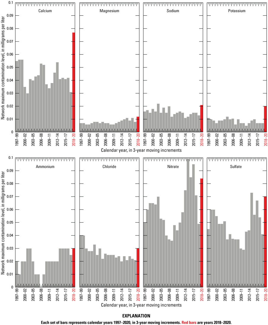
Network maximum contamination levels for National Trends Network analytes calculated using 3-year moving increments, 1997–2020.
The NADP changed its sampling protocol during 2020 by lining the buckets with clean-room grade, disposable plastic bags in order to decrease shipping, washing, and packaging costs associated with the reusable buckets. Extensive laboratory testing of the bags by the CAL did not reveal contamination issues (Camille Danielson, WSLH, oral and written commun., 2020). Therefore, the contamination might be introduced by field handling of the bags during the installation procedure or when the bag-lined buckets are switched out at the time of sample collection when both the bag-lined bucket containing the previous week’s sample and the fresh bag-lined bucket are briefly exposed to the atmosphere. The effect that the contamination has on the samples is likely negligible as studies by the ISWS in 2015 found no significant difference between analyte concentrations samples collected using unlined and bag-lined buckets (Mark Rhodes, Illinois State Water Survey, written commun., 2016). However, the NMCL increases determined in 2018–20 indicate a substantial introduction of contamination during this period, wherein the WSLH began to analyze field-audit samples and bag liners were introduced to the sampling protocol (fig. 1).
Analyte Losses
Maximum values for analyte losses in NTN samples were higher in 2018–20 than for 2017–19 periods for all analytes except calcium and potassium (table 1). Maximum values for nitrate and ammonium losses during 2017–19, were similar to those for the previous six years, but losses of these reactive nitrogen species increased slightly during 2018–20 (fig. 2A). The MDL for ammonium increased by a factor of 17 between 2019 and 2020, and this change alone could mathematically account for estimated increases in ammonium loss. The CAL detected minor losses of nitrate and ammonium from low-concentration solutions that were allowed to dwell in bag liners in laboratory studies (Camille Danielson, WSLH, oral and written commun. 2020). Increased ammonium loss could also be due to the switch to bag-lined bucket sampling protocols mentioned above. Hydrogen ion maximum loss increased slightly from 2.5 microequivalents per liter (μeq/L) during 2016–18 to 3.0 μeq/L during 2017–19 and then increased more dramatically, to 4.5 μeq/L, during 2018–20 (fig. 2B). The maximum hydrogen-ion loss of 4.5 μeq/L is greater than the median valid NTN hydrogen-ion concentration (3.090 μeq/L) measured during 2018–20. Calcium and magnesium NMCL also increased during this same period. This change might indicate buffering of hydrogen ion with dust contamination introduced by the switch to a bag-lined bucket sampling protocol implemented during 2020. However, the 3-year median and upper quartile calcium concentrations in NTN samples also increased by 9 and 19 percent, respectively, between 2016–18 and 2018–20. Therefore, the increased calcium contamination and concurrent loss of hydrogen ion in NTN samples might be related to changing environmental conditions, such as a shift to a drier climate and dustier troposphere (Brahney and others, 2015; Hedin and Likens, 1996). Finally, the CAL identified a pH calibration error in early 2020 that caused some hydrogen-ion concentrations to have a slightly high bias, which might have accentuated the bucket-minus-bottle hydrogen-ion concentration differences during the 2018–20 period.
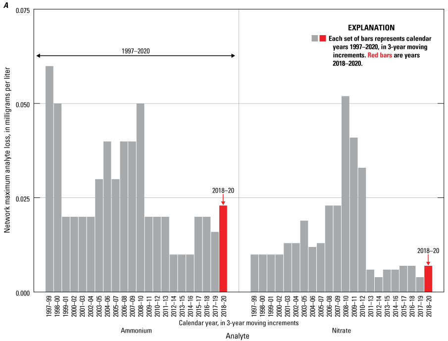
Maximum loss of A, ammonium and nitrate, and B, hydrogen ion from weekly National Trends Network samples calculated using 3-year moving increments, 1997–2020.
National Trends Network Interlaboratory Comparison Program
The CAL’s analytical variability and bias were evaluated with respect to other international monitoring networks in the Northern Hemisphere. There was no attempt to account for the different onsite sampling protocols used by different monitoring networks. Eleven laboratories participated in the interlaboratory comparison program during 2019–20: (1) Asia Center for Air Pollution Research (ACAP) in Niigata-shi, Japan; (2) Prairie Research Institute, Illinois State Water Survey, in Champaign, Ill., (PRI, formerly ICAL during 2017–18); (3) Wood Group, Inc. (WOOD), in Gainesville, Florida; (4) Ontario Ministry of Environment and Climate Change–Dorset Chemistry Laboratory (MOECC), in Dorset, Ontario, Canada; (5) Environment and Climate Change Canada, Science and Technology Branch (ECST) in Downsview, Ontario, Canada; (6) Norwegian Institute for Air Research (NILU) in Kjeller, Norway; (7) Carey Institute of Ecosystem Studies (CIES), in Millbrook, New York; (8) U.S. Department of Agriculture, Forest Service Northern Research Station (NRS), in Durham, New Hampshire; (9) RTI International (RTI), in Research Triangle Park, North Carolina, (10) Universidad Nacional Autónoma de México (UNAM), Centro de Ciencias de la Atmósfera, in Mexico City, Mexico; and (11) NADP CAL, Wisconsin State Laboratory of Hygiene, in Madison, Wisc. (CAL, formerly WCAL during 2017–18).
Each of the participating laboratories received four samples from PCQA every month for chemical analysis. Three types of samples were used in the interlaboratory comparison program: (1) synthetic standard reference samples prepared by PCQA, which are traceable to National Institute of Standards and Technology (NIST) reference materials (NIST-traceable materials); (2) de-ionized water blank samples prepared by PCQA; and (3) natural wet-deposition samples collected at NTN sites, blended by CAL, and sent to PCQA for shipping to the laboratories as blind samples (Wetherbee and Martin, 2017). Synthetic precipitation samples used in the interlaboratory comparison program were made from stock solutions prepared by High Purity Standards, Charleston, South Carolina. Natural samples were filtered through 0.45-micrometer filters; contained in 60-, 125-, and 250-milliliter polyethylene bottles by CAL; and shipped in chilled, insulated containers to the PCQA to enhance stability of nutrient analytes—ammonium, nitrate, and sulfate—in the samples (Tchobanoglous and Schroeder, 1987; U.S. Geological Survey, 2002).
Median concentrations of calcium, magnesium, sodium, potassium, ammonium, chloride, nitrate, sulfate, and hydrogen ion and median specific conductance were computed by solution from the data submitted by all participating laboratories. The median values were considered to be equal to the MPV. Censored concentration values reported as less than the MDL were included in the estimation of MPV for each solution using the Kaplan-Meier method (Helsel, 2012). The largest percentages of censored concentration values in the samples analyzed during 2019–20 were those for magnesium and potassium, most commonly in natural wet-deposition samples.
The MPV for the synthetic precipitation solutions and the number of samples analyzed per solution are listed in table 2 by solution identifier: SP1B, SP15B, SP15C, SP18B, SP18D, SP2B, SP21B, SP22B. Data from each laboratory were compared against these MPV to evaluate bias. In previous years, the PRI, NRS, CIES, and CAL laboratories analyzed the samples for bromide, but bromide was eliminated as an NTN analyte in 2019. Therefore, data for bromide concentrations reported to USGS by the participating laboratories were not analyzed or reported herein. The RTI laboratory routinely analyzed the samples only for chloride, nitrate, sulfate, sodium, potassium, and ammonium. The ECST, NRS, and RTI laboratories did not analyze the samples for specific conductance. The NRS and RTI laboratories did not measure pH for any of the samples. Data are missing for March – December 2020 for ECST and for all of 2020 for UNAM because the laboratories were closed due to the COVID-19 pandemic.
Table 2.
Most probable values for analytes in synthetic precipitation solutions used in the 2019–20 National Trends Network interlaboratory comparison program.[Data are available in Wetherbee (2022). Ca2+, calcium; Mg2+, magnesium; Na+, sodium; K+, potassium; NH4+, ammonium; Cl-, chloride; NO3-, nitrate; SO42-, sulfate; H+, hydrogen ion; all units in milligrams per liter except hydrogen ion (microequivalents per liter) and specific conductance (microsiemens per centimeter at 25 degrees Celsius)]
Adjustments were made to the PCQA interlaboratory comparison program’s normal schedule of sample types during 2020. Sample shipments to participating laboratories were delayed for several months during the winter and spring due to the COVID-19 pandemic. Delayed shipments of samples to the participating laboratories were fulfilled in the following manner. Instead of mixing new synthetic solutions, a large number of natural-matrix water samples were obtained from the USGS Standard Reference Sample (SRS) archive and repackaged for analysis by the PCQA participating laboratories (https://bqs.usgs.gov/srs/). This change was helpful for catching up with the PCQA sample shipping schedule, and it provided an opportunity to test the suitability and stability of SRS samples as a potential substitute for the current PCQA interlaboratory-comparison program protocol. Analysis of the data obtained from the participating laboratories, however, revealed highly variable analytical results for the SRS samples, indicating potential instability, especially but not exclusively the results for ammonium and nitrate. Therefore, the SRS samples were determined to be unsuitable for the PCQA program, and the results obtained for the archive samples were excluded from the statistical and graphical analysis presented herein. Data for the SRS samples are available in the data release for this report (Wetherbee, 2022).
Bias and Variability
Interlaboratory bias for the participating laboratories was evaluated using the following methods: (1) comparison of the medians of the differences between laboratory results and MPV, (2) hypothesis testing using the sign test, and (3) comparison of laboratory results for de-ionized water samples. The arithmetic signs of the median differences indicate whether the reported results for each constituent are positively or negatively biased. The sign test null hypothesis is the true median of the reported-minus-MPV differences is zero. Test results were evaluated at the α=0.05 significance level for a two-tailed test.
Calculated variation between laboratories was compared using the f-psig ratios (eq. 6). Analytical detection limits are reported for each laboratory in table 3. Results for variability and bias within the analytical data reported by each of the participating laboratories are presented in tables 4 and 5. Shaded values in tables 4 and 5 identify analytes for which bias was found to be both statistically (α=0.05) and practically important. For this program, statistically significant bias was determined to be of practical importance only when the absolute value of the median relative concentration difference was greater than the participating laboratory’s analytical method detection limit.
Table 3.
Analytical detection limits for laboratories participating in the U.S. Geological Survey interlaboratory-comparison program for the National Atmospheric Deposition Program 2019–20.[Data are available in Wetherbee (2022). Participating laboratories: ACAP, Asia Center for Air Pollution Research; CAL, Central Analytical Laboratory, Wisconsin State Laboratory of Hygiene; CIES, Carey Institute of Ecosystem Studies; ECST, Environment and Climate Change Canada Science and Technology Branch; MOECC, Ontario Ministry of Environment and Climate Change; NILU, Norwegian Institute for Air Research; NRS, U.S, Department of Agriculture Forest Service Northern Research Station; ; PRI, Prairie Research Institute, Illinois State Water Survey; RTI, RTI International; UNAM, Universidad Nacional Autónoma de México; WOOD, Wood Group, Inc.; mg/L, milligram per liter]
Table 4.
Median differences between reported constituent concentrations and most probable values for synthetic wet-deposition samples, 2019 interlaboratory comparison program.[Data are available in Wetherbee (2022). ACAP, Asia Center for Air Pollution Research; CAL, Central Analytical Laboratory, Wisconsin State Laboratory of Hygiene; CIES, Carey Institute of Ecosystem Studies; ECST, Environment and Climate Change Canada Science and Technology Branch; MOECC, Ontario Ministry of Environment and Climate Change; NILU, Norwegian Institute for Air Research; NRS, U.S. Forest Service Northern Research Station; PRI, Prairie Research Institute, Illinois State Water Survey; RTI, RTI International; UNAM, Universidad Nacional Autónoma de México; WOOD, Wood Group, Inc.; all units in milligrams per liter, except hydrogen ion (microequivalents per liter) and specific conductance (microsiemens per centimeter at 25 degrees Celsius); overall f-psig, f-pseudosigma for all participating laboratories; median diff., median of differences between each laboratory's individual results and the most probable value during 2019, in analyte units; f-psig ratio, ratio of each individual laboratory's f-pseudosigma to the overall f-pseudosigma; sign test p-value, probability of rejecting the null hypothesis: “The true median of the differences between laboratory results and the most probable value is zero,” when true; values are shaded where median bias is greater than the method detection limit (table 3) and statistically significant (α=0.05) (Kanji, 2006); —, not calculated; <, less than]
Table 5.
Median differences between reported constituent concentrations and most probable values for synthetic wet-deposition samples, 2020 interlaboratory comparison program.[Data are available in Wetherbee (2022). ACAP, Asia Center for Air Pollution Research; CAL, Central Analytical Laboratory, Wisconsin State Laboratory of Hygiene; CIES, Carey Institute of Ecosystem Studies; ECST, Environment and Climate Change Canada Science and Technology Branch; MOECC, Ontario Ministry of Environment and Climate Change; NILU, Norwegian Institute for Air Research; NRS, U.S. Forest Service Northern Research Station; PRI, Prairie Research Institute, Illinois State Water Survey; RTI, RTI International; WOOD, Wood Group, Inc.; all units in milligrams per liter except hydrogen ion (microequivalents per liter) and specific conductance (microsiemens per centimeter at 25 degrees Celsius); overall f-psig, f-pseudosigma for all participating laboratories; median diff., median of differences between each laboratory's individual results and the most probable value during 2020, in analyte units; f-psig ratio, ratio of each individual laboratory's f-pseudosigma to the overall f-pseudosigma; sign test p-value, probability of rejecting the null hypothesis: “The true median of the differences between laboratory results and the most probable value is zero,” when true; values are shaded where median bias is greater than the method detection limit (table 3) and statistically significant (α=0.05) (Kanji, 2006); —, not calculated; <, less than]
During 2019–20, the interlaboratory-comparison results for CAL and WOOD indicated no practically significant bias (in other words, greater than the absolute values of the detection limits) for all analytes. For the other participating laboratories, the results indicated practically significant bias for the following analytes by year.
-
ACAP—calcium, magnesium, and sodium in 2019 and 2020, and a large bias for sulfate in 2020 only.
-
CIES—calcium and nitrate in 2019, and calcium, magnesium, sodium, ammonium, and nitrate in 2020.
-
ECST—calcium, sodium, potassium, and sulfate only in 2019.
-
MOECC—chloride and nitrate in 2019, and increased bias for calcium, magnesium, sodium, chloride, nitrate and sulfate in 2020.
-
NILU—ammonium in 2020 only.
-
NRS—magnesium and sodium in 2019, and sodium, potassium, ammonium, chloride, nitrate, and sulfate in 2020.
-
PRI—calcium, sodium, and sulfate in 2019, and sodium, chloride, and sulfate in 2020.
-
RTI—sodium and nitrate in 2019 only.
The CAL results demonstrated low variability for all analytes in 2019 – 20 except for hydrogen ion in 2019. A pH instrument calibration problem was corrected in 2020, which yielded much improved results as the f-psig ratio for CAL hydrogen ion data was reduced from 2.03 (2019) to 0.60 (2020) (tables 4 and 5). Results for the ECST, RTI, and WOOD laboratories indicated generally low variability for most analytes during 2019, but higher variability than overall was indicated for sulfate (ECST and PRI) and hydrogen ion (PRI and WOOD) during 2020 (tables 4 and 5). Variability for MOECC, NILU, and NRS was generally higher than overall during 2020. Results that were missing owing to the temporary closures of the ECST and UNAM laboratories during 2020 might have influenced the increases in variability and bias observed during the study period for some laboratories.
The interlaboratory-comparison program shipped four blank samples to participating laboratories each year during 2019 and three blanks during 2020 (table 6). The CAL reported concentrations above analytical detection limits for calcium (1 sample), potassium (2 samples), ammonium (3 samples), chloride (2 samples), and nitrate (1 sample) during 2019. The CAL reported concentrations above analytical detection limits for potassium and sulfate for 1 sample during 2020. The ACAP laboratory reported detections for all constituents for at least 1 blank per analyte during 2019 and for at least 2 blanks per analyte during 2020. The CIES laboratory reported at least one detection for all analytes in blank samples during the study period. The ECST laboratory reported detections for potassium in all blank samples during 2019. The MOECC laboratory reported detections for ammonium and nitrate in all blank samples during 2019 and 1 detection for each analyte for blank samples during 2020. No results were reported above analytical detection limits for blank samples for the RTI laboratory during the study period. The NILU laboratory reported 1 detection for sodium and chloride, and the WOOD laboratory reported 1 detection for magnesium for blank samples during the study period. The PRI laboratory reported detections for calcium (3 samples), potassium (2 samples), and ammonium (3 samples) during 2019, and for calcium, magnesium, chloride, and sulfate for 2 blank samples during 2020. The NRS laboratory reported detections for ammonium, chloride, nitrate, and sulfate for at least 3 blanks during 2019 and for at least 2 blanks during 2020.
Table 6.
Number of analyte determinations greater than the method detection limits for deionized water samples, 2019–20.[Data are available in Wetherbee (2022). Participating laboratories: ACAP, Asia Center for Air Pollution Research; CAL, Central Analytical Laboratory, Wisconsin State Laboratory of Hygiene; CIES, Carey Institute of Ecosystem Studies; ECST, Environment and Climate Change Canada Science and Technology Branch; MOECC, Ontario Ministry of Environment and Climate Change; NILU, Norwegian Institute for Air Research; NRS, U.S, Department of Agriculture Forest Service Northern Research Service; PRI, Prairie Research Institute, Illinois State Water Survey; RTI, RTI International; UNAM, Universidad Nacional Autónoma de México; WOOD, Wood Group, Inc.; —, no data; *, n=1 sample for ECST]
Control Charts
Each participating laboratory’s results were compared to the MPV over time in control charts. Analyte determinations that exceeded the control limits (± 3 f-psig) during 2019–20 are summarized in table 7. Each laboratory was provided with its own sets of control charts. The CAL values were mostly within the ±3 f-pseudosigma statistical control limits for all analytes, but an instrument calibration error positively biased the synthetic precipitation sample results in 2019. Meanwhile, analyses of the natural precipitation samples, which had higher pH than the synthetic samples, produced results within statistical control. The pH instrument calibration protocol was corrected in 2020, which improved the CAL’s results for hydrogen-ion analysis.
Table 7.
Number of analyte determinations outside ±3 f-pseudosigma statistical control limits, by participating laboratory, 2019–20.[Data are available in Wetherbee (2022). n, number of samples analyzed; Ca, calcium; Mg, magnesium; Na, sodium; K, potassium; NH4, ammonium; Cl, chloride; NO3, nitrate; SO4, sulfate; Sc, specific conductance at 25 degrees Celsius; H, hydrogen ion concentration from pH; ACAP, Asia Center for Air Pollution Research; CAL, Central Analytical Laboratory, Wisconsin State Laboratory of Hygiene; CIES, Carey Institute of Ecosystem Studies; ECST, Environment and Climate Change Canada Science and Technology Branch; MOECC, Ontario Ministry of Environment and Climate Change; NILU, Norwegian Institute for Air Research; NRS, U.S, Department of Agriculture Forest Service Northern Research Service; PRI, Prairie Research Institute, Illinois State Water Survey; RTI, RTI International; UNAM, Universidad Nacional Autónoma de México; WOOD, Wood Group, Inc.; —, no data; *, ECST only participated in January and February during 2020]
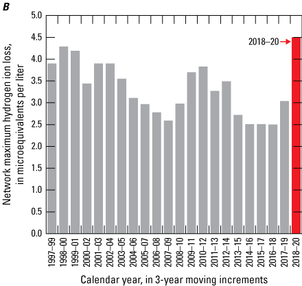
Control charts for the CAL for 2019–20 are shown in figures 3A and 3B. Points in the control charts are color- and symbol-coded by solution type to provide a visual indication of potential solution-specific bias. During 2019, trends in bias ranging from slightly negative in early 2019 to slightly positive in late 2019 are illustrated in figure 3A for calcium, ammonium, chloride, nitrate, and especially sulfate. During 2020, no bias was observed in the control charts for ammonium, chloride, nitrate, and sulfate. The CAL results for magnesium, sodium, potassium (fig. 3A), indicated a slightly positive bias during 2019–20. The CAL’s specific conductance results indicated a positive bias during 2019 but no bias during 2020 (fig. 3B).
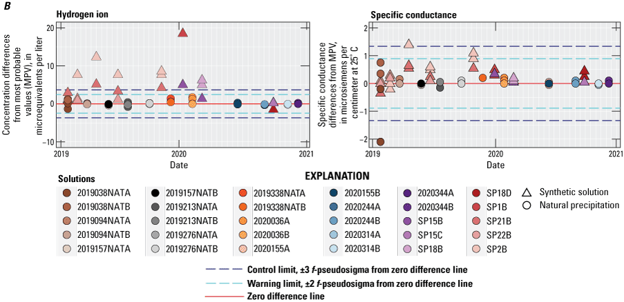
Differences between concentration values reported by the Central Analytical Laboratory and the median concentration values (MPV) for all participating laboratories in the interlaboratory comparison program for the National Trends Network, 2019–20, for A, calcium, magnesium, sodium, potassium, ammonium, chloride, nitrate, sulfate; and B, hydrogen-ion concentrations and specific conductance. Data are available in Wetherbee (2022).
Mercury Deposition Network Quality Assurance Programs
The USGS operated a system blank program and an interlaboratory comparison program for the MDN during 2019–20. Protocols for the PCQA external QA programs for MDN are described in detail by Wetherbee and Martin (2017). The MDN system blank program is similar to the NTN field audit program, whereby the effects of onsite environmental exposure, handling, and shipping on sample contamination are evaluated. The MDN interlaboratory comparison program quantified variability and bias of MDN analytical data provided by the Mercury Analytical Laboratory (HAL) at the Wisconsin State Laboratory of Hygiene for 2019–20.
System Blank Program
The MDN site operators received system blank samples from PCQA for processing during 2019–20, but no samples were shipped to MDN sites in 2018 to allow for transfer of HAL operations from its former location at Eurofins Frontier Global Sciences to the Wisconsin State Laboratory of Hygiene. After a week without wet deposition at a site, operators poured one-half of the volume of the system blank solution through the glass sample train. The glass sample train consists of a funnel, which collects the precipitation, and a thistle tube, which drains the precipitation into the sample bottle. The solution that washed through the sample train is called the system blank sample, and the solution remaining in the original sample bottle is called the bottle sample. Both system blank and bottle samples were sent together to HAL for total mercury (Hg) analysis.
Of the 78 active MDN sites that received system blank samples in 2019 and again in 2020, operators at 33 sites either processed samples or returned a postcard to PCQA indicating no dry (precipitation-free) weeks during 2019, and operators at 39 sites responded during 2020. Although no system blank samples were shipped in 2018, 7 samples were shipped in 2017 and analyzed in 2018 before the HAL moved to WSLH later that year, and these 7 samples were included in the calculations for the 2017–19 and 2018–20 periods. In all, 68 system blank samples were processed with accompanying bottle samples for chemical analysis at the HAL, and data for these system blank sample pairs were received by PCQA for assessment of sample contamination and stability.
Network Maximum Contamination Levels for Mercury
The NMCL for total Hg were calculated from the system blank data using a 3-year moving window, starting with 2004–06. NMCL during the 2017–19 and 2018–20 periods were not greater than 1.000 ng/L and 0.926 ng/L, respectively. These concentrations are less than the first percentile of all MDN sample data collected during 2018–20, which is 1.383 ng/L. Therefore, contamination in MDN samples during 2017–20 was less than the first percentile of all MDN concentrations with 90-percent confidence, and no more than 10 percent of the MDN samples had contamination concentrations in excess of approximately 1.000 ng/L with 90-percent confidence (Robert Larson, NADP Program Office, Wisconsin State Laboratory of Hygiene, written commun., 2021). These values were calculated with only 7 samples submitted during 2018 because no system blank samples were shipped to the field in 2018 to accommodate transition of the HAL operations from the Eurofins Frontier Global Sciences laboratory to the Wisconsin State Laboratory of Hygiene.
Mass of Mercury Contamination
The mass of Hg contamination in each system blank sample was calculated as follows:
where[HgSB] is the total Hg concentration in system blank sample, in nanograms per liter;
VolumeSB is the volume of system blank sample, in liters;
[HgBot] is the total Hg concentration in the bottle sample, in nanograms per liter; and
VolumeBot is the volume of the bottle sample, in liters.
Next, the UCLs of the percentiles of the system sample minus bottle sample Hg mass differences were calculated. The maximum estimated contaminant mass per sample decreased slightly from 0.095 ng Hg during 2016–18 to 0.087 ng Hg during 2017–19, and then the NMCL increased to 0.089 ng Hg during 2018–20. The MDN NMCL for total Hg contamination mass per sample has been stable at approximately 0.1 ng per sample over the past six years (table 8).
Table 8.
Three-year moving network maximum contamination levels and 90-percent upper confidence limits at the 50th, 75th, and 90th percentiles of total mercury contamination mass in system blank samples, 2004–20.[Data are available in Wetherbee (2020a; 2020b; 2022). %, percent; UCL, upper confidence limit; Hg, total mercury; ng Hg, nanogram of mercury; ng total Hg/L, total nanograms of mercury per liter; *, n=7 samples for 2018 because no samples were shipped to accommodate laboratory transition]
Mercury Deposition Network Interlaboratory Comparison Program
The objective of the MDN interlaboratory comparison program is to compare the variability and bias of HAL analytical results with results from laboratories supporting various monitoring networks, while not accounting for the different onsite protocols used by different networks. Eleven laboratories participated in the program during the study period: (1) HAL at Wisconsin State Laboratory of Hygiene, in Madison, Wisconsin; (2) Department of Atmospheric Science, National Central University (DASNCU), in Jhong-Li District, Taoyuan City, Taiwan; (3) Flett Research, Ltd. (FRL), in Winnipeg, Manitoba, Canada; (4) Swedish Environmental Institute (IVL) in Goteborg, Sweden; (5) Quebec Laboratory for Environmental Testing (LEEQ or QLET) in Montreal, Quebec, Canada; (6) North Shore Analytical, Inc., (NSA) in Duluth, Minnesota; (7) USGS Mercury Research Laboratory (WML) in Middleton, Wisconsin; (8) National Institute for Minamata Disease (NIMD), Minamata, Kumamoto, Japan; (9) Environmental Research and Training Center (ERTC), Amphoe Klong Luang, Pathumthani, Thailand; (10) Gwangju Institute of Science & Technology (GIST), Gwuangju, Republic of Korea; and (11) Kangwon National University (KNU), Gangwon-do, Republic of Korea. During 2020, the GIST and KNU laboratories discontinued participation. The WML laboratory provided results obtained by two independent analytical methods: an automated method presented as laboratory identifier WMLA, and a manual method presented by the identifier WMLM. All laboratories analyzed the water samples for low levels of Hg using atomic fluorescence spectrometry methods similar to U.S. Environmental Protection Agency Method 1631 (U.S. Environmental Protection Agency, 2002).
During 2019, each participating laboratory received two samples per month consisting of 1-percent (volume:volume) hydrochloric acid blanks and mercuric nitrate spiked at four different concentrations in a 1-percent hydrochloric acid matrix. During 2020, each participating laboratory received 24 samples, but the monthly shipping schedule was interrupted. Samples scheduled for March and April were shipped in June. The laboratories were instructed to analyze the samples as soon as they were received to promote accurate time representation of the data, but this was not possible for all laboratories due to the effect of the COVID-19 pandemic on laboratory operations. Additionally, the normal sample schedule for 2020 was altered by including samples from the USGS standard reference sample (SRS; https://bqs.usgs.gov/srs/) archive, consisting of samples HG57, HG60, and HG68. These samples were included to determine the suitability of the SRS as a substitute QC program for the MDN. However, the analytical results for these samples obtained from the laboratories indicated substantial variability and bias for the SRS samples, and the data were omitted from the control charts and other statistical analyses to determine laboratory performance. Analytical results for the SRS samples are included in the data release (Wetherbee, 2022).
All samples were single-blind samples, whereby the chemical analyst knew that the sample was a quality-control sample but did not know the total Hg concentrations in the samples. The medians of all the concentration values obtained from the participating laboratories were considered to be MPV, which are listed in table 9.
Table 9.
Most probable values for total mercury in spiked solutions and hydrochloric acid blank samples used for the U.S. Geological Survey Mercury Deposition Network interlaboratory comparison program, 2019–20.[Data available in Wetherbee (2022). Hg, total mercury; MPV, most probable value; ng/L, nanogram per liter; %, percent; HCl, hydrochloric acid; BLANK, mercury-free de-ionized water with 1% HCl by volume; MP1–MP4, mercuric nitrate standard diluted to target concentrations in 1% HCl; Blank MPV estimated by Kaplan-Meier method in R – NADA package because of large number of censored values]
Control Charts
Total Hg analysis data submitted by each laboratory were compared to MPV for each of the solutions. Differences between reported results and MPV were plotted on annual control charts, which were delivered to each laboratory by PCQA. Control charts include warning limits placed at ±2 f-psig and control limits at ±3 f-psig from the zero-difference line. Values outside the control limits represent periods when a laboratory’s analyses were considered to be out of statistical control. The HAL’s control chart is shown in figure 4.
The HAL’s control chart shows that most results were within statistical control during 2019, but three results were outside of the -3 f-psig control limit. During 2020, four results were outside of the -2 f-psig warning limit, and three results were outside of the -3 f-psig control limit (fig. 4). A negative bias in HAL MDN concentrations of approximately -1 ng/L is indicated by the control chart for the study period.
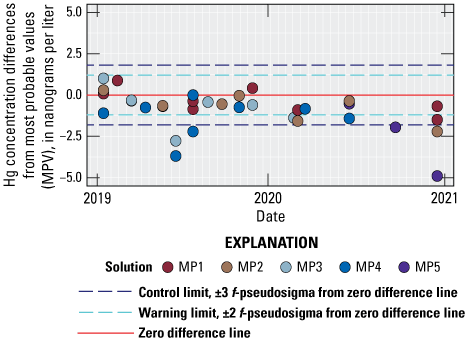
Differences between total mercury concentrations reported by the Mercury (Hg) Analytical Laboratory at the Wisconsin State Laboratory of Hygiene and the median concentration values for all participating laboratories in the interlaboratory comparison program for the Mercury Deposition Network, 2019–20, excluding results for USGS SRS test solutions HG57, HG60, and HG68 analyzed in 2020. Data are available in Wetherbee (2022).
Interlaboratory Variability and Bias
Each laboratory’s results for variability and bias are summarized in table 10. Methods for evaluation of the data are analogous to those for the NTN interlaboratory comparison program. The f-psig ratio was computed as shown in equation 6 and expressed as a decimal for each laboratory, whereby an f-psig ratio larger than 1.00 indicates that results provided by a laboratory exhibited higher variability than the overall variability among the participating laboratories; a ratio smaller than 1.00 indicates less variability than overall. Annual overall f-psig values were 0.693 ng/L and 0.612 ng/L for 2019 and 2020, respectively, for the concentration ranges indicated by the MPV in table 9. The arithmetic signs of the median differences indicate whether the results of analyses for total mercury were positively or negatively biased. Interlaboratory bias was evaluated for statistical significance using the sign test for location of a median (Kanji, 2006; Wetherbee and others, 2014).
Table 10.
Differences between reported concentrations and most probable values for total mercury determinations, Mercury Deposition Network interlaboratory comparison program, 2019–20.[Data are aavailable in Wetherbee (2022). ng/L, nanogram per liter; overall f-psig, f-pseudosigma for all participating laboratories; median diff., median of differences between each laboratory's individual results and the most probable values for each solution; sign test p-value, probability of rejecting the null hypothesis: “The true median of the differences between laboratory results and the most probable value is zero,” when true; f-psig ratio, ratio of each individual laboratory's f-pseudosigma to the overall f-pseudosigma; HAL, Mercury Analytical Laboratory at Wisconsin State Laboratory of Hygiene; DASNCU, Department of Atmospheric Sciences, National Central University (Taiwan); ERTC, Environmental Research and Training Center (Thailand); FRL, Flett Research, Ltd. (Canada); GIST, Gwangju Institute of Science and Technology (Republic of Korea); IVL, Swedish Environmental Research Institute; KNU, Kangwon National University (Republic of Korea); LEEQ, Quebec Laboratory of Environmental Testing (Canada); NIMD, National Institute for Minamata Disease (Japan); NSA, North Shore Analytical, Inc.; WML(A/M), U.S. Geological Survey Mercury Research Laboratory (A, automated method / M, manual method); n.d., no data; <, less than; statistical warning limits are ±2 overall f-psig, statistical control limits are ±3 overall f-psig]
Results in table 10 indicate that during 2019, the HAL’s analytical variability was lower than the overall interlaboratory variability (f-psig ratio of 0.80) and similar to that of the KNU, LEEQ, and WMLA laboratories. During 2020, however, the HAL’s analytical variability was greater than that of all other participating laboratories (f-psig ratio of 1.94). The HAL results for 2019 indicated low negative bias with a small median difference from the MPV of -0.398 ng/L that was not significantly different from zero, which is indicated by the sign test (p=0.078). During 2020, the HAL bias increased, indicated by a median difference from the MPV of -1.120 ng/L, which was significantly different from zero (p<0.001). The HAL’s absolute median difference is less than the first percentile of all weekly MDN total Hg concentrations measured during 2018–20 (1.38 ng/L). Annual bias estimates for all of the laboratories are negligible compared to concentrations of total Hg determined for the MDN during 2018–20 (Robert Larson, NADP Program Office, Wisconsin State Laboratory of Hygiene, written commun., 2021).
The results imply that the HAL’s analytical performance declined between 2019 and 2020. Several factors should be considered, however, when applying the HAL’s performance in this program to an assessment of MDN data quality for 2020. The HAL participates in a performance testing program conducted by Environment and Climate Change Canada, and the HAL’s results for this program were acceptable in 2020 (Christa Dahman, Wisconsin State Laboratory of Hygiene, written and oral commun., 2021). Laboratory operations were affected by the COVID-19 pandemic as analysis schedules were interrupted by staff furloughs. The LEEQ laboratory did not participate in the program, and the GIST and KNU laboratories discontinued their participation in 2020, which could have affected the MPV, but likely only slightly. There were also minor shifts in performance, both positively and negatively, for the DASNCU, ERTC, NSA, and WMLM laboratories during 2020. This information is provided for consideration of potential corrective actions for the HAL.
Analytical Results for Blank Samples
Interlaboratory comparison results for the analyses of blank samples for mercury in 2019-20 are shown in table 11. Four blind blank samples were shipped to each laboratory annually. Minimum reporting levels (MRL) differ among the laboratories and were less than or equal to 0.20 ng/L during 2019–20. The HAL reported zero values above the detection limit of 0.20 ng/L for blank samples during 2019 and one value above detection during 2020. As shown for results in previous years, results of blank analyses indicate that Hg contamination at HAL during the study period was low (Wetherbee and Martin, 2016; 2020). Therefore, most Hg contamination in MDN samples, which was estimated using the system blanks, was likely introduced in the field.
Table 11.
Number of total mercury determinations greater than the method detection limits for blank samples, Mercury Deposition Network interlaboratory comparison program, 2019–20.[Data available in Wetherbee (2022). Four determinations per year per laboratory with exception of WMLA in 2019; HAL, Mercury Analytical Laboratory, Wisconsin State Laboratory of Hygiene.; DASNCU, Department of Atmospheric Sciences, National Central University (Taiwan); ERTC, Environmental Research and Training Center (Thailand); FRL, Flett Research, Ltd. (Canada); GIST, Gwangju Institute of Science and Technology (Republic of Korea); IVL, Swedish Environmental Research Institute; KNU, Kangwon National University (Republic of Korea); LEEQ, Quebec Laboratory of Environmental Testing (Canada); NIMD, National Institute for Minamata Disease (Japan); NSA, North Shore Analytical, Inc.; WML(A/M), U.S. Geological Survey Mercury Research Laboratory (A, automated method / M, manual method);ng/L, nanogram per liter; nd, no data]
1 Laboratories did not participate in the 2020 interlaboratory-comparison program.
2WMLA analyzed 2 blanks in 2019.
Data Quality Assessment
This report presents an assessment of the overall data quality for NADP precipitation chemistry measurements. With the exception of the biased hydrogen-ion concentration measurements in 2019, the results indicate no particular bias or variability in the data that would prevent or require modifications in the application of the data by NADP and its data users for evaluation of spatial variation and temporal trends in atmospheric deposition. The results presented herein should be considered in combination with information provided in NADP Quality Assurance Reports available on the NADP web site (University of Wisconsin-Madison, Wisconsin State Laboratory of Hygiene, 2020a; 2020b; 2020c; 2021a; 2021b).
Summary
The U.S. Geological Survey’s (USGS) Precipitation Chemistry Quality Assurance (PCQA) project implemented two programs to provide external quality assurance monitoring for the National Atmospheric Deposition Program’s (NADP) National Trends Network (NTN) and two additional programs to provide external quality assurance monitoring for the NADP Mercury Deposition Network (MDN) during 2019–20. The field audit program assessed the effects of sample collection-site exposure, sample handling, and sample shipping protocols on the results of laboratory chemical analyses of NTN samples; the system blank program assessed the same effects for MDN samples. Two interlaboratory comparison programs assessed the bias and variability of the chemical analysis data from the Central Analytical Laboratory (CAL), Mercury Analytical Laboratory (HAL), and other participating laboratories that analyze precipitation samples for major ions, nutrients, and trace levels of mercury (Hg).
This report presents quality-assessment information for 2020, the year of the COVID-19 pandemic outbreak. Many of the laboratories’ median concentration differences were lower in 2020 than in 2019, indicating improvement in accuracy. However, interruptions in laboratory operations owing to the pandemic and changes in PCQA sample preparation and shipping protocols during 2020 may have affected the results presented in this report, and those factors should be considered when using this information to evaluate the quality of NADP data for the NTN and MDN samples that were collected during 2020. The results indicate that the NADP data obtained during the 2019–20 period were of acceptable quality for their intended uses per the 2016 NADP Network Quality Assurance Plan and the 2020 NADP Laboratory Quality Assurance Plan (NADP, 2016; 2020).
National Trends Network
Field audit results for 2019–20 indicate that Network Maximum Contamination Levels (NMCLs) for NTN samples increased significantly (α=0.05) since 2017–18 for all analytes. Notable increases in the NMCLs for NTN from 2017–19 to 2018–20, were 0.031 to 0.077 milligrams per liter (mg/L) for calcium, 0.049 to 0.084 mg/L for nitrate, 0.041 to 0.070 mg/L for sulfate, and 1.3 to 3.4 microequivalents per liter (μeq/L) for hydrogen ion. Variable levels of sample contamination over the past 10 years are small in terms of absolute concentrations. However, the 2018–20 NMCLs for calcium, magnesium, potassium, and hydrogen ion were greater than the 25th percentile concentrations, respectively, in NTN samples during the same period. The NMCLs for chloride (0.030 mg/L), nitrate (0.084 mg/L), and sulfate (0.070 mg/L), were at the 14th, 8th, and 4th NTN concentration percentiles, respectively. This program also estimated the maximum loss of ammonium, nitrate, and hydrogen ion in weekly NTN samples. Ammonium maximum loss increased from 0.016 mg/L (2017–19) to 0.023 mg/L (2018–20). Nitrate maximum loss was negligible at 0.004 – 0.007 mg/L, and hydrogen ion maximum loss increased from 3.0 to 4.5 (μeq/L) during the study period. Hydrogen-ion maximum loss was stable between 2014–17 and then increased to 2.50 μeq/L during 2016–18 (Wetherbee and Martin, 2020). The marked increase in hydrogen-ion loss in NTN samples over the past several years is coincident with increasing calcium contamination, indicating possible buffering of sample pH by dust contamination, which was likely introduced in the field, but not in the laboratory.
For samples collected and analyzed in 2019, statistically significant bias was observed for CAL laboratory analyses for calcium, sodium, potassium, chloride, hydrogen ion and specific conductance. For samples collected and analyzed in 2020, statistically significant bias was observed for CAL analyses for calcium, magnesium, sodium, potassium, hydrogen ion and specific conductance. The magnitudes of the biases were less than the detection limits and not practically significant. The CAL results indicated low variability relative to that of the other laboratories participating in the intercomparison program except for hydrogen ion during 2019, when the CAL’s pH variability was two times higher than the overall (all laboratories) variability. A calibration error for pH analyses was discovered by the CAL and corrected in 2020. The Asia Center for Air Pollution Research (ACAP), Environment and Climate Change Canada Science and Technology Branch (ECST), Prairie Research Institute (PRI), Research Triangle International (RTI), and Wood Group, Inc. (WOOD) laboratories demonstrated generally low variability for all constituents except hydrogen ion (ACAP, PRI, and WOOD) and sulfate (PRI) during the study period.
The participating laboratories received four de-ionized water blanks for analysis in 2019 and three blanks in 2020. Very few concentrations were reported above analytical detection limits for blank samples for the Norwegian Institute for Air Research (NILU), Universidad Nacional Autónoma de México (UNAM), and RTI laboratories during 2019–20, but these laboratories use reporting limits that are unchanging from year to year instead of actual detection limits, which likely vary below the reporting limits. The ACAP laboratory reported detections for all constituents in at least one blank per analyte in both years. The CAL reported detections for calcium (1) potassium (2), ammonium (3), chloride (2), and nitrate (1) during 2019, and for potassium (1) and sulfate (1) during 2020. Laboratories that reported a relatively higher number of concentrations above their analytical detection limits were Cary Institute for Ecosystem Studies (CIES), Northern Research Station (NRS), and PRI, which report newly calculated and relatively low analytical detection limits every year.
Analyte determinations that exceeded statistical control limits (± 3 f-pseudosigma) for CAL during 2019–20 include magnesium (1), sodium (1), potassium (1), ammonium (3), chloride (3), nitrate (3), sulfate (4), specific conductance (4), and hydrogen ion (15). The exceedances for hydrogen ion occurred predominantly in analyses performed during 2019 due to a pH calibration error that was corrected during 2020. The interlaboratory-comparison program results indicated relatively greater numbers of analyses exceeding the control limits for the Ontario Ministry of Environment and Climate Change (MOECC), NRS, and UNAM laboratories.
Mercury Deposition Network
The MDN NMCL for total Hg decreased from 1.010 ng/L during 2016–18 to 1.000 ng/L during 2017–19 and to 0.926 ng/L during 2018–20. The maximum contamination in MDN samples during 2018–20 was not greater than 0.926 ng/L with 90-percent confidence, and no more than 10 percent of the MDN samples had contamination concentrations exceeding 0.926 ng/L with 90-percent confidence. This concentration is less than the first percentile of all MDN weekly total Hg concentrations measured during 2018–20 (1.383 ng/L). Median differences from the MPV were -0.398 and -1.120 ng/L for 2019 and 2020, respectively, which were also less than the first percentile of all weekly MDN total Hg concentrations. The HAL’s negative bias was statistically significant only for 2020 results.
The HAL’s control chart for 2019–20 for the interlaboratory comparison program indicates a negative bias of approximately 1 ng/L for total Hg concentration analyses. Three results were outside the -3 f-psig control limits each year during 2019–20. Four results were outside of the -2 f-psig warning limit during 2020. In comparison with the participating laboratories, the HAL’s total Hg analyses were characterized by less variability than overall (all laboratories) during 2019 with an f-psig ratio of 0.80. The HAL results indicated variability nearly two times higher than overall during 2020 with an f-psig ratio of 1.94. Participating laboratories analyzed four blank samples containing no Hg each year. The HAL reported no values above the detection limit of 0.20 ng/L during 2019 and one value above detection during 2020 for blank samples.
References Cited
Brahney, J., Mahowald, N., Ward, D.S., Ballantyne, A.P., and Neff, J.C., 2015, Is atmospheric phosphorus pollution altering global alpine lake stoichiometry?: Global Biogeochemical Cycles, v. 29, p. 1369–1383, accessed January 24, 2023, at https://doi.org/10.1002/2015GB005137.
Hahn, G.J., and Meeker, W.Q., 1991, Statistical intervals—A guide for practitioners: New York, John Wiley & Sons, 392 p. [Also available at https://doi.org/10.1002/9780470316771.]
Kanji, G.K., 2006, 100 statistical tests (3rd ed.): New Delhi, Sage Publications Ltd., 242 p. [Also available at https://doi.org/10.4135/9781849208499.]
Latysh, N.E., and Wetherbee, G.A., 2005, External quality assurance programs managed by the U.S. Geological Survey in support of the National Atmospheric Deposition Program/National Trends Network: U.S. Geological Survey Open-File Report 2005–1024, 66 p., accessed January 31, 2018, at https://doi.org/10.3133/ofr20051024.
Latysh, N.E., and Wetherbee, G.A., 2007, External quality assurance programs managed by the U.S. Geological Survey in support of the National Atmospheric Deposition Program/Mercury Deposition Network: U.S. Geological Survey Open-File Report 2007–1170, 33 p., accessed January 24, 2023, at https://doi.org/10.3133/ofr20071170.
National Atmospheric Deposition Program [NADP], 2016, NADP Network Quality Assurance Plan, version 1.8, 29 p., accessed February 17, 2023, at https://nadp.slh.wisc.edu/wp-content/uploads/2021/04/NADP_Network_Quality_Assurance_Plan.pdf.
National Atmospheric Deposition Program [NADP], 2020, NADP Laboratory Quality Assurance Plan, NADP Mercury and Central Analytical Laboratories, 78 p., accessed February 17, 2023, at https://nadp.slh.wisc.edu/wp-content/uploads/2021/04/QAPNADPLab2020.pdf.
R Development Core Team, 2018, R—A language and environment for statistical computing, version 3.5.2 (Eggshell Igloos): Vienna, Austria, R Foundation for Statistical Computing, software release, accessed August 5, 2021, at http://www.R-project.org/.
R Development Core Team, 2021, R—A language and environment for statistical computing, version 4.0.4 (Lost Library Book): Vienna, Austria, R Foundation for Statistical Computing, software release, accessed August 5, 2021, at http://www.R-project.org/.
SAS Institute, Inc., 2016, SAS software version 9.4: Cary, N.C., SAS Institute Inc., accessed January 26, 2023, at https://support.sas.com/software/94/.
University of Wisconsin-Madison, Wisconsin State Laboratory of Hygiene, 2020a, 2019 Quality Assurance Report: National Atmospheric Deposition Program, Central Analytical Laboratory, 33 p., accessed January 25, 2022, at https://nadp.slh.wisc.edu/wp-content/uploads/2021/04/cal_2019_QAR.pdf.
University of Wisconsin-Madison, Wisconsin State Laboratory of Hygiene, 2020b, 2019 Quality Assurance Report National Atmospheric Deposition Program, Mercury Deposition Network, Mercury Analytical Laboratory, accessed January 25, 2022, at https://nadp.slh.wisc.edu/wp-content/uploads/2021/04/HAL_QAR_2019.pdf.
University of Wisconsin-Madison, Wisconsin State Laboratory of Hygiene, 2020c, Laboratory Quality Assurance Plan, National Atmospheric Deposition Program, Mercury and Central Analytical Laboratories, accessed January 25, 2022, at https://nadp.slh.wisc.edu/wp-content/uploads/2021/04/QAPNADPLab2020.pdf.
University of Wisconsin-Madison, Wisconsin State Laboratory of Hygiene, 2021a, 2020 Quality Assurance Report: National Atmospheric Deposition Program, Central Analytical Laboratory, 47 p., accessed January 25, 2022, at https://nadp.slh.wisc.edu/wp-content/uploads/2021/10/cal_2020_QAR.pdf.
University of Wisconsin-Madison, Wisconsin State Laboratory of Hygiene, 2021b, 2020 Quality Assurance Report: National Atmospheric Deposition Program, Mercury Analytical Laboratory, 26 p., accessed January 25, 2022, at https://nadp.slh.wisc.edu/wp-content/uploads/2021/10/hal_2020_QAR.pdf.
U.S. Environmental Protection Agency, 2002, Method 1631, revision E—Mercury in water by oxidation, purge and trap, and cold vapor atomic fluorescence spectrometry: U.S. Environmental Protection Agency, Office of Water report EPA–821–R–02–019, 38 p., accessed May 6, 2014, at https://water.epa.gov/scitech/methods/cwa/metals/mercury/upload/2007_07_10_methods_method_mercury_1631.pdf.
U.S. Geological Survey, 2002, Processing of Water Samples (ver. 2, April 2002), Wilde, F.D., ed.: U.S. Geological Survey Techniques of Water-Resources Investigations, book 9, chap A5, 90 p., accessed April 15, 2020, at https://doi.org/10.3133/twri09A5.
Wetherbee, G.A., 2020a, Data for the U.S. Geological Survey precipitation chemistry quality assurance project for the National Atmospheric Deposition Program, 1978–2017: U.S. Geological Survey data release, accessed January 10, 2022, at https://doi.org/10.5066/P94RC4GD.
Wetherbee, G.A., 2020b, U.S. Geological Survey precipitation chemistry quality assurance project data 2017–2018: U.S. Geological Survey data release, accessed May 1, 2021, at https://doi.org/10.5066/P9ZKXD8N.
Wetherbee, G.A., 2022, U.S. Geological Survey precipitation chemistry quality assurance project data 2019–2020: U.S. Geological Survey data release, accessed December 1, 2022, at https://doi.org/10.5066/P9B119QP.
Wetherbee, G.A., Latysh, N.E., Greene, S.M., and Chesney, T.A., 2010, U.S. Geological Survey external quality-assurance project report to the National Atmospheric Deposition Program/National Trends Network and Mercury Deposition Network, 2007–08: Champaign, Ill., National Atmospheric Deposition Program Quality Assurance Report 2010-01 and Illinois State Water Survey Miscellaneous Publication 190, 82 p., accessed April 15, 2020, at https://www.isws.illinois.edu/pubdoc/MP/ISWSMP-190.pdf.
Wetherbee, G.A., Martin, RA., Rhodes, M.F., and Chesney, T.A., 2014, External quality-assurance project report for the National Atmospheric Deposition Program/National Trends Network and Mercury Deposition Network for 2009–2010: U.S. Geological Survey Scientific Investigations Report 2013–5147, 53 p., accessed April 15, 2020, at https://doi.org/10.3133/sir20135147.
Wetherbee, G.A., and Martin, RA., 2016, External quality assurance project report for the National Atmospheric Deposition Program’s National Trends Network and Mercury Deposition Network, 2013–14: U.S. Geological Survey Scientific Investigations Report 2016–5069, 22 p., accessed April 15, 2020, at https://doi.org/10.3133/sir20165069.
Wetherbee, G.A., and Martin, RA., 2017, Updated operational protocols for the U.S. Geological Survey precipitation chemistry quality assurance project in support of the National Atmospheric Deposition Program: U.S. Geological Survey Open-File Report 2016–1213, 18 p., accessed January 31, 2018, at https://doi.org/10.3133/ofr20161213.
Wetherbee, G.A., and Martin, RA., 2020, External quality assurance project report for the National Atmospheric Deposition Program’s National Trends Network and Mercury Deposition Network, 2017–18: U.S. Geological Survey Scientific Investigations Report 2020-5084, 31 p., accessed August 5, 2021, at https://doi.org/10.3133/sir20205084.
Conversion Factors
International System of Units to U.S. customary units
Temperature in degrees Celsius (°C) may be converted to degrees Fahrenheit (°F) as °F = (1.8 × °C) + 32.
Supplemental Information
Specific conductance is given in microsiemens per centimeter at 25 degrees Celsius (µS/cm at 25 °C).
Concentrations of chemical constituents in water are given in either milligrams per liter (mg/L), microequivalents per liter (µeq/L), or nanograms per liter (ng/L).
α, alpha, is the maximum probability of incorrect rejection of the null hypothesis.
100(p)th is the percentile equal to 100 times a value of p, for example, 100 × (.9) = 90th percentile.
Absolute value of x = |x|, where x takes the form of numerical values or algebraic expressions.
Study period, calendar year 2019–20.
Water year (WY) is the 12-month period from October 1 through September 30 of the following year and is designated by the calendar year in which it ends.
Abbreviations
μeq/L
microequivalents per liter
ACAP
Asia Center for Air Pollution Research
CAL
Central Analytical Laboratory, Wisconsin State Laboratory of Hygiene, University of Wisconsin, Madison
CIES
Carey Institute of Ecosystem Studies
CVAFS
Cold vapor atomic fluorescence spectroscopy
DASNCU
Department of Atmospheric Sciences, National Central University (Taiwan)
ECST
Environment and Climate Change Canada (formerly [2015–16] Environment Canada) Science and Technology Branch
ERTC
Environmental Research Training Center (Thailand)
ETI
Environmental Technologies, Inc., Fort Collins, Colorado
f-psig
f-pseudosigma
FRL
Flett Research, Limited (Canada)
GIST
Gwangju Institute of Science & Technology (South Korea)
HAL
Mercury Analytical Laboratory, Wisconsin State Laboratory of Hygiene, University of Wisconsin, Madison
HCl
hydrochloric acid
Hg
mercury
ICAL
Central Analytical Laboratory, University of Illinois, Illinois State Water Survey
ISWS
Illinois State Water Survey
IVL
IVL Swedish Environmental Research Institute (Sweden)
KNU
Kangwon National University (South Korea)
LEEQ
Quebec Laboratory for Environmental Testing (Canada), also known as QLET
MDL
method detection limit
MDN
Mercury Deposition Network
MOECC
Ministry of Environment and Climate Change—Dorset Chemistry Laboratory (Canada)
MPV
most probable value
MRL
minimum reporting level
NADP
National Atmospheric Deposition Program
NILU
Norwegian Institute for Air Research (Norway)
NIMD
National Institute for Minamata Disease (Japan)
NIST
National Institute of Standards and Technology
NMCL
network maximum contamination level
Noah IV
Environmental Technologies, Inc. model Noah IV precipitation gage
NRS
U.S. Department of Agriculture Forest Service, Northern Research Station, Durham, New Hampshire
NSA
North Shore Analytical, Inc.
NTN
National Trends Network
PCQA
Precipitation Chemistry Quality Assurance project
PO
Program Office for National Atmospheric Deposition Program
PRI
Prairie Research Institute, University of Illinois, Urbana-Champaign, Illinois
QA
quality assurance
RTI
Research Triangle Institute, International
RVP
Readiness Verification Plan
SRS
standard reference sample
UCL
upper confidence limit
UNAM
Universidad Nacional Autónoma de México, Centro de Ciencias de la Atmósfera (University of Mexico, Center for Atmospheric Sciences, Mexico City, Mexico)
USGS
U.S. Geological Survey
WML
U.S. Geological Survey Wisconsin Mercury Laboratory
WOOD
Wood Group, Incorporated
WSLH
Wisconsin State Laboratory of Hygiene, University of Wisconsin, Madison
Publishing support provided by the Science Publishing Network,
Denver and Reston Publishing Service Center
For more information concerning the research in this report, contact the
Director, Observing Systems Division
USGS Hydrologic Instrumentation Facility
Buildings 2101 2204 HIF - Stennis Space Center
Bay St Louis, MS 39529
800-382-0634
Suggested Citation
Wetherbee, G.A., Martin, RA., and Liethen, A., 2023, External quality-assurance project report for the National Atmospheric Deposition Program’s National Trends Network and Mercury Deposition Network, 2019–20: U.S. Geological Survey Scientific Investigations Report 2023–5045, 29 p., https://doi.org/10.3133/sir20235045.
ISSN: 2328-0328 (online)
Study Area
| Publication type | Report |
|---|---|
| Publication Subtype | USGS Numbered Series |
| Title | External quality-assurance project report for the National Atmospheric Deposition Program’s National Trends Network and Mercury Deposition Network, 2019–20 |
| Series title | Scientific Investigations Report |
| Series number | 2023-5045 |
| DOI | 10.3133/sir20235045 |
| Year Published | 2023 |
| Language | English |
| Publisher | U.S. Geological Survey |
| Publisher location | Reston VA |
| Contributing office(s) | WMA - Observing Systems Division |
| Description | Report: vii, 29 p.; 3 Data Releases |
| Country | United States |
| Online Only (Y/N) | Y |
| Google Analytic Metrics | Metrics page |