

Range-wide Population Trend Analysis for Greater Sage-Grouse (Centrocercus urophasianus)—Updated 1960–2022
Links
- Document: Report (13 MB pdf) , HTML , XML
- Data Release: Trends and a targeted annual warning system for greater sage-grouse in the western United States (ver. 2.0, May 2023)
- Download citation as: RIS | Dublin Core
Acknowledgments
We conducted this update and original modeling analysis in close consultation with the Bureau of Land Management, Sage-Grouse and Columbian Sharp-tailed Grouse Technical Committee for the Western Association of Fish and Wildlife Agencies, and the U.S. Fish and Wildlife Service. We thank John Tull (U.S. Fish and Wildlife Service) and Jonathan Rose (U.S. Geological Survey) for helpful comments in reviewing this data report in its entirety. We extend gratitude for the cooperation of personnel from 11 western state wildlife agencies, who provided feedback at various stages on uses of lek data, modeling methods, and constructive reviews at various stages of production. Specifically, we value the contributions from T. Remington (Western Association of Fish and Wildlife Agencies), S. Stiver (Western Association of Fish and Wildlife Agencies), S. Espinosa (Nevada Department of Wildlife), K. Griffin (Colorado Parks and Wildlife), K. Miller (California Department of Fish and Wildlife), A. Moser (Idaho Department of Fish and Game), M. Kemner (Idaho Department of Fish and Game), A. Cook (Utah Division of Wildlife Resources), L. Foster (Oregon Department of Fish and Wildlife), J. Kolar (North Dakota Game and Fish Department), T. Runia (South Dakota Department of Game, Fish and Parks), M. Schroeder (Washington Department of Fish and Wildlife), N. Whitford (Wyoming Game and Fish Department), C. Wightman (Montana Department of Fish, Wildlife and Parks), B. Wakeling (Montana Department of Fish, Wildlife and Parks), S. Vold (Oregon Department of Fish and Wildlife), and M. Cline (Oregon Department of Fish and Wildlife). We thank K. Andrle (Nevada Department of Wildlife), K. McGowan (Nevada Sagebrush Ecosystem Technical Team), M. Magaletti, A. Kosic, P. Winters (Bureau of Land Management), J. Tull (U.S. Fish and Wildlife Service), K. Borland, M. Nelson (U.S. Forest Service), S. Abele (U.S. Fish and Wildlife Service), S. Gardner, and B. Ehler (California Department of Fish and Wildlife) for their input throughout the initial components of this study. This project could not have been completed without the financial support of the Bureau of Land Management, U.S. Geological Survey, and the funds for the pilot efforts that were provided by the Bureau of Land Management-Nevada and Nevada Department of Wildlife.
Introduction
As of the turn of the twenty-first century, sage-grouse occupied roughly half of their former historical range (Schroeder and others, 2004; Miller and others, 2011) and populations have subsequently experienced marked declines in many parts of their current range (Garton and others, 2011; Western Association of Fish and Wildlife Agencies, 2015). In a recent study led by the U.S. Geological Survey (USGS), in collaboration with the Bureau of Land Management (BLM) and the Western Association of Fish and Wildlife Agencies (WAFWA), a Bayesian state-space modeling framework was used, which revealed an approximately 3.1-percent annual average decline range-wide that dates back to the 1960s (Coates and others, 2021). However, variation in trends was described across different spatial and temporal scales.
Decades of literature have attributed sage-grouse population declines to loss and fragmentation of sagebrush communities as well as to a suite of environmental stressors (Connelly and others, 2004; Schroeder and others, 2004; Doherty and others, 2016). Since 1999, sage-grouse have been petitioned for legal protection under the Endangered Species Act (ESA) on nine occasions, and actions to conserve and restore sage-grouse habitats are now central to guiding land-management actions and policies across most of the western United States. Specifically, in recent years, the resource needs of sage-grouse have been used to help guide management actions aimed at improving conditions in sagebrush ecosystems, with resultant practices thought to benefit other sagebrush-dependent species (Rowland and others, 2006; Hanser and Knick, 2011; Dinkins and others, 2021). Sage-grouse are considered an indicator for the function of sagebrush ecosystems and an umbrella for the protection of other sagebrush-obligate or sagebrush-dependent species because of their near complete reliance on sagebrush ecosystems (Rich and Altman, 2001; Rich and others, 2005; Rowland and others, 2006; Hanser and Knick, 2011). However, some recent literature indicates that some less associated species might not be well covered by the sage-grouse umbrella (Carlisle and others, 2018). Importantly, several federal resource management plan amendments accompanying the U.S. Fish and Wildlife Service (USFWS) “not warranted” 2015 ESA listing determination called for greater integration of sage-grouse management into their land-use planning and specifically, identifying how to implement adaptive management. An unprecedented level of conservation effort and planning among federal (Bureau of Land Management, 2015; U.S. Department of Agriculture Forest Service, 2015a, b19), state, and private stakeholders was identified as the primary driver for the USFWS decision in their most recent status assessment (U.S. Fish and Wildlife Service, 2015).
The purpose of this report is to provide updated results on sage-grouse population trends across their geographical range of western United States. This report reflects previous modeling methodology (Coates and others, 2021, 2022a) and includes additional data to inform population trends through 2022. A detailed description of data collection and compilation, population clustering methods to identify spatial extents, and trend modeling methodologies were provided in the first three objectives described in Coates and others (2021). Additional methodologies developed since Coates and others (2021) are described in Coates and others (2022a). The USGS, in cooperation with the WAFWA and BLM, are providing this scientific information to fulfill a prominent information gap that will help inform status assessments of sage-grouse population trends and conservation management strategies.
Study Area
Our study extent consisted of the geographic range of sage-grouse in the United States and was described previously in Coates and others (2021). Briefly, this area represents the sagebrush biome occurring across western North America and extending east from the Sierra Nevada/Cascade mountain ranges to the western regions of the Great Plains of the United States. The vegetation communities vary with precipitation, temperature, soils, topographic position, and elevation (Miller and others, 2011). The most abundant shrub species include sagebrush (Artemisia spp.), with less abundant non-sagebrush species such as rabbitbrush (Chrysothamnus spp.), horsebrush (Tetradymia spp.), greasewood (Sarcobatus spp.), common snowberry (Symphoricarpos spp.), serviceberry (Amelanchier spp.), fourwing saltbush (Atriplex spp.), and bitterbrush (Purshia spp.). The primary herbaceous species include wheatgrass (Agropyron spp.), fescue (Festuca spp.), bluegrass (Poa spp.), needlegrass (Stipa spp.), bromegrass (Bromus spp.), and squirreltail (Sitanion spp.), whereas less abundant forb species include phlox (Phlox spp.), milk-vetch (Astragalus spp.), and fleabane (Erigeron spp.).
Data Compilation and Inputs
All digitized field observations of sage-grouse lek counts since 1953 were compiled from all state wildlife agencies that monitored sage-grouse populations and entered into a single unified database. We worked with each agency to ensure the fullest understanding of the data to maximize the number of appropriate records kept in the database, we addressed spatial errors, and we reviewed all data products with state wildlife staff members of the WAFWA Sage and Columbian Sharp-tailed Grouse Technical Committee. Data compilation rules and detailed methodology used in this analysis was published in Coates and others (2021) and O’Donnell and others (2021). The additional years of data (up to 2022) used to update this trend analysis followed the exact quality assessment and quality control (QA/QC) measures described in the previous publications. Furthermore, state-specific summaries of number and percentage (relative to maximum value in any given year) of leks and observations retained followed the sequential application of Rules 1–6 described in appendix 2 of Coates and others (2021). Using all the rules for selecting data appropriate to population modeling, we retained 106,920 observations across 5,403 leks. The sage-grouse lek data used in this update either are not available or have limited availability owing to unique restrictions held by each state (data are managed by 11 western states and are not public due to the sensitivity of the species and state regulations, policies, or laws). Contact the Greater Sage-Grouse Technical Team of the WAFWA or individual state wildlife agencies (see the “Acknowledgments” section) for more information.
Changes in population abundance are affected by environmental factors that operate on multiple spatial and temporal scales, which follow ecological, rather than geopolitical, boundaries. Hence, we examined population trends across biologically relevant and hierarchically nested units to improve the detection of factors driving change across various spatial scales. We grouped sage-grouse lek sites into hierarchical nested clusters or populations using least-cost minimum spanning trees, a clustering algorithm, and a suite of relevant biotic and abiotic spatial products described in Coates and others (2021). Briefly, we selected two cluster levels to represent a fine (neighborhood cluster, NC) and broad spatial scale (climate cluster, CC) in trend analyses. Model output included estimated abundance () and intrinsic rates of population change () at the lek level.
Range-wide Sage-Grouse Population Model
Detailed formulation of the sage-grouse population model was described in Coates and others (2021). Analytical updates that (1) identify population nadirs (lowest points within cycles) at the lek (breeding ground) and neighborhood cluster (group of leks) spatial scales and (2) truncate prior distributions on rate of change in apparent abundance values to more realistic boundaries for leks with missing data are described in Coates and others (2022a). Briefly, we used a Bayesian state-space model (SSM) that relied on Markov chain Monte Carlo (MCMC) sampling to derive posterior probability distributions (PD) of and using lek count data across the sage-grouse geographical range. This approach allowed inferences for each lek, as well as higher-order, and nested spatial extents such as NC and CC, during each year of the time series. Advantages and assumptions inherent to the SSM approach were described in Coates and others (2021, 2022a).
Modification—Additional Year of Data
The most recent published trend analysis included data from 1960 to 2021 (Coates and others, 2022a, 2022b5). In this report, we updated the model to include lek count data collected during 2022 for all 11 western states across sage-grouse geographic range. Because SSMs estimate changes in population size using a Markov process (state at time t+1 depends on state at time t), trends reported in Coates and others (2022a) may experience slight shifts with the inclusion of the new year of data. This version of the analysis supersedes previous reports and represents current trends across different spatial extents (for instance, leks, NCs, and CCs) and temporal periods (for instance, 2022 back-in-time to each population nadir) across the geographic range of sage-grouse.
Range-wide Population Trends
Our model fit the observed data well (Bayesian p-value=0.50). Median from the SSM revealed six distinct range-wide population nadirs across the 63 years of data, which were 1966, 1975, 1986, 1996, 2002, and 2013. The range-wide, across-years, mean male count was 17.4 per lek (95-percent confidence interval=17.3–17.6) based on data restricted to trend analyses. The number of years for complete oscillation periods (nadir-to-nadir) was relatively consistent across periods (average=9.2; 95-percent CRI=6.3–11.0; table 1). Model estimates revealed evidence of range-wide decline, on average, from every historic abundance nadir to 2021 (fig. 1; table 2); for example, the average annual for short (19 years, two oscillations), medium (35 years, four oscillations), and long (55 years, six oscillations) temporal scales was 0.971 (median; 95-percent CRI=0.969–0.973), 0.970 (median; 95-percent CRI=0.967–0.971), and 0.971 (median; 95-percent CRI=0.969–0.973), respectively. These trends imply declines of 40.9, 65.0, and 79.6 percent, relative to population sizes observed 19, 35, and 55 years earlier, respectively. In an earlier version of the model (Coates and others, 2021), we specified the final nadir for all populations using the final year of the dataset (2019), which was the lowest point of for most populations at that time. A more recent report provided an update of the original analysis and included years 2020 and 2021 (Coates and others, 2022a, 2022b5). In that report, researchers concluded that not all populations had reached a nadir in 2019. With the additional year of count data (2022) provided in this report, we have identified 2021 as the final nadir for several populations. However, increases in abundance during 2022 were modest for most of those populations, making 2021 a tentative final nadir. Trends estimated at CC (fig. 2) and NC (fig. 3) scales are generally consistent with the previous report (Coates and others 2022a). Specific to NCs, we estimated median to be less than 1.0 for 87.4, 91.0, and 97.4 percent across short, medium, and long temporal scales, respectively, throughout the sage-grouse range.
Table 1.
Identified years of population abundance nadirs (lowest points within cycles) used to define temporal scales (recent to long-term) of population trend estimates across different climate clusters (A–F) and range-wide for greater sage-grouse (Centrocercus urophasianus) in the western United States.[Range-wide estimated abundance nadirs were 1966, 1975, 1986, 1996, 2002, and 2013 that reflect long, medium/long, medium, short/medium, short, and recent, respectively, temporal scales for inferring trends. Abbreviations: CC, climate cluster; A, Bi-State area; B, Washington area; C, Jackson Hole, Wyoming area; D, eastern area; E, Great Basin area; F, western Wyoming area]
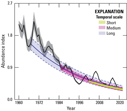
Abundance index (calculated as divided by 63-year mean of ) of greater sage-grouse (Centrocercus urophasianus) across their range from lek observations used to model population trends during 1960–2022. Median estimates (solid colored lines) and 95-percent credible limits (dashed colored lines) of abundance trend across temporal scales: Short (two periods), Medium (four periods), and Long (six periods), right to left. Black trend line represents median estimates. Colored areas represent 95-percent credible limits of trend estimates. Grey shaded areas represent 95-percent credible limits on abundance index.
Table 2.
Greater sage-grouse (Centrocercus urophasianus) average annual rate of population change () across six different temporal scales that corresponded to differing periods of oscillation (recent [one period], short [two periods], short/medium [three periods], medium [four periods], medium/long [five periods], long [six periods]) for each climate cluster in the western United States (see table 1).[Abbreviations: CC, climate cluster; A, Bi-State area; B, Washington area; C, Jackson Hole, Wyoming area; D, eastern area; E, Great Basin area; F, western Wyoming area; , estimated finite rate of population change]
Lengths of temporal scales were defined by population abundance nadirs that varied for each climate cluster (see table 1). Estimates for each period represent median with 95-percent credible intervals in parentheses.
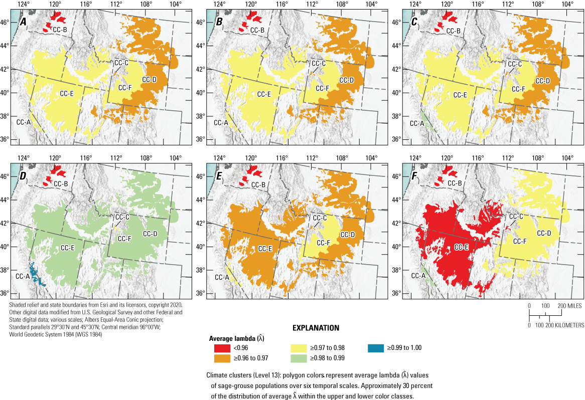
Range-wide spatial estimates of average annual rate of change () in abundance of greater sage-grouse (Centrocercus urophasianus) across six temporal scales based on periods of oscillation: A, Long (six periods); B, Medium/long (five periods); C, Medium (four periods); D, Short/medium (three periods); E, Short (two periods); and F, Recent (one period) for each climate cluster (CCs; A–F). Map image is the intellectual property of Esri and is used herein under license. Copyright © 2020 Esri and its licensors. All rights reserved. Abbreviations: <, less than; ≥, greater than or equal to.
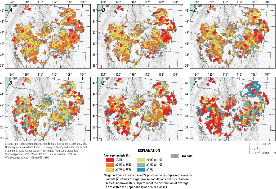
Range-wide spatial estimates of average annual population rate of change () in abundance of greater sage-grouse (Centrocercus urophasianus) across six temporal scales based on periods of oscillation: A, Long (six periods); B, Medium/long (five periods); C, Medium (four periods); D, Short/medium (three periods); E, Short (two periods); and F, Recent (one period) for each neighborhood cluster. Map image is the intellectual property of Esri and is used herein under license. Copyright© 2020 Esri and its licensors. All rights reserved. Abbreviations: <, less than; ≥, greater than or equal to.
Climate Cluster Population Trends
Climate cluster A (CC-A; Bi-State area) consisted of 11 NCs that encompassed 726,907 hectares (ha). Two NCs did not have sufficient lek data to estimate trends. Climate cluster A consisted of 93 leks, representing approximately 1 percent of the range-wide database. After QA/QC, 57 leks met criteria for use in the SSM (table 2), totaling 1,683 field observations. Mean male count was 20.2 (95-percent confidence interval=18.9–21.6). For CC-A, we estimated six population abundance nadirs that dated back to 1960 and included nadirs of 1969, 1977, 1983, 1995, 2002, and 2008 (table 1). We estimated at the short (2002–19, two periods of oscillation over 17 years), medium (1983–2019, four periods over 36 years), and long temporal scales (1969–2019, six periods over 50 years) as 0.975 (95-percent CRI=0.963–0.984), 0.988 (95-percent CRI=0.974–0.997), and 0.978 (95-percent CRI=0.967–0.986), respectively (fig. 4A; table 2). During the past 17, 36, and 50 years, sage-grouse populations have experienced declines in abundance equal to 33.9, 34.6, and 66.6 percent, respectively. We estimated median to be less than 1.0 for all NCs across short, medium, and long temporal scales, respectively.
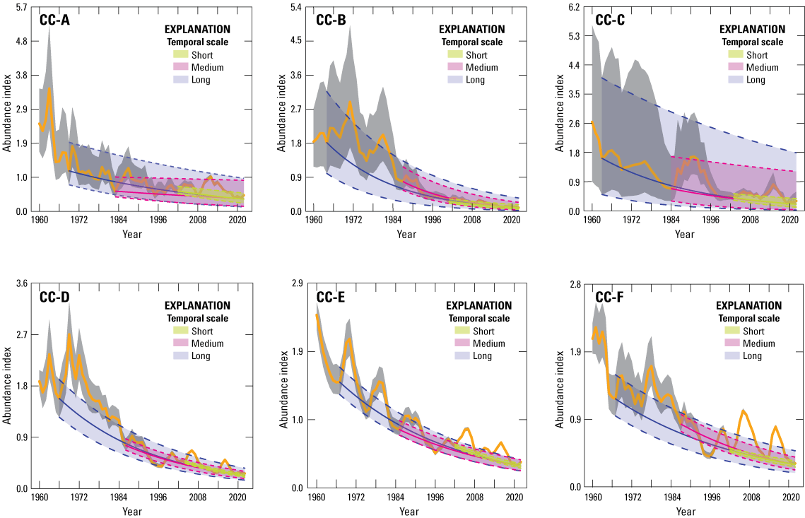
Abundance index (calculated as divided by 63-year mean of ) of greater sage-grouse (Centrocercus urophasianus) in climate clusters (CCs): A, (CC-A; Bi-State area); B, (CC-B; Washington area); C, (CC-C; Jackson Hole, Wyoming area); D, (CC-D; Eastern area); E, (CC-E; Great Basin area); and F, (CC-F; western Wyoming area). Lek observations were used to model population trends during 1960–2022. Median estimates (solid colored lines) and 95-percent credible limits (dashed colored lines) of abundance trends across temporal scales based on periods of oscillation: Short (two periods), Medium (four periods), and Long (six periods), right to left. Colored areas represent 95-percent credible limits of trend estimates. Black lines and grey shaded areas represent median and 95-percent credible limits on abundance index, respectively.
Climate cluster B (CC-B; Washington area) consisted of four NCs that encompassed 1,139,954 ha. One NC did not have sufficient lek data to estimate trends. Climate cluster B consisted of 113 leks, representing approximately 1.3 percent of the lek database. After QA/QC, 69 leks met criteria for use in the state-space trend model (table 2), totaling 1,167 field observations. Mean male count was 13.8 (95-percent confidence interval=13.0–14.7). We estimated six population abundance nadirs that dated back to 1960 and included 1964, 1976, 1987, 1995, 2001, and 2008 (table 1). We estimated at the short (2001–22, two periods of oscillation over 21 years), medium (1987–2022, four periods over 35 years), and long-temporal scales (1964–2022, six periods over 58 years) as 0.958 (95-percent CRI=0.946–0.972), 0.945 (95-percent CRI=0.934–0.957), and 0.953 (95-percent CRI=0.943–0.963), respectively (fig. 4B; table 2). During the past 21, 35, and 58 years, sage-grouse populations have experienced declines in abundance equal to 57.1, 85.2, and 93.5 percent, respectively. We estimated median to be less than 1.0 for all NCs across short, medium, and long temporal scales, respectively.
Climate cluster C (CC-C; Jackson Hole, Wyoming area) consisted of two NCs that encompassed 66,733 ha. Climate cluster C consisted of 17 leks, representing approximately 0.2 percent of the lek database. After QA/QC, 14 leks met criteria for use in the SSM (table 2), totaling 329 field observations. Mean male count was 13.9 (95-percent confidence interval=12.2–15.6). For CC-C, we estimated population abundance nadirs during 1963, 1969, 1984, 1999, 2003, and 2011 (table 1). We estimated at the short (2003–19, two periods of oscillation over 16 years), medium (1984–2019, four periods over 35 years), and long-temporal scales (1963–2019, six periods over 56 years) as 0.964 (95-percent CRI=0.945–0.983), 0.969 (95-percent CRI=0.945–0.992), and 0.966 (95-percent CRI=0.950–0.986), respectively. During the past 16, 35, and 56 years, sage-grouse populations have experienced declines in abundance equal to 42.7, 65.8, and 85.5 percent, respectively (fig. 4C; table 2). We estimated median to be less than 1.0 for all NCs across this temporal scale.
Climate cluster D (CC-D; eastern area) consisted of 169 NCs that encompassed 25,920,530 ha. There were 26 NCs that did not have sufficient lek data for trend estimates. Climate cluster D consisted of 3,042 leks, representing approximately 35.0 percent of the lek database. After QA/QC, 1,918 leks met criteria for use in the SSM (table 2) and totaled 37,738 field observations. Mean male count was 16.0 (95-percent confidence interval=15.8–16.2). For CC-D, we estimated six population abundance nadirs that dated back to 1960 and included 1966, 1981, 1986, 1997, 2004, and 2014 (table 1). We estimated at the short (2004–19, two periods of oscillation over 13 years), medium (1986–2019, four periods over 31 years), and long temporal scales (1966–2019, six periods over 51 years) as 0.961 (95-percent CRI=0.957–0.965), 0.967 (95-percent CRI=0.963–0.971), and 0.966 (95-percent CRI=0.963–0.970), respectively (fig. 4D; table 2). During the past 13, 31, and 51 years, sage-grouse populations have experienced declines in abundance equal to 42.6, 65.5, and 83.2 percent, respectively. We estimated median to be less than 1.0 for 91.0, 95.1, and 99.3 percent of NCs across short, medium, and long temporal scales, respectively.
Climate cluster E (CC-E; Great Basin area) consisted of 241 NCs that encompassed 34,627,182 ha. There were 22 NCs that lacked sufficient data to estimate trends. Climate cluster E consisted of 4,154 leks, representing approximately 47.8 percent of the lek database. After QA/QC, 2,332 leks met criteria for use in the SSM (table 2) and totaled 43,543 field observations. Mean male count was 16.1 (95-percent confidence interval=15.9–16.3). For CC-E, we estimated six population abundance nadirs that dated back to 1960 and included 1967, 1975, 1985, 1996, 2002, and 2013 (table 1). We estimated at the short (2002–21, two periods of oscillation over 19 years), medium (1985–2021, four periods over 36 years), and long temporal scales (1967–2021, six periods over 54 years) as 0.967 (95-percent CRI=0.965–0.970), 0.973 (95-percent CRI=0.970–0.976), and 0.971 (95-percent CRI=0.969–0.974), respectively (fig. 4E; table 2). During the past 19, 36, and 54 years, sage-grouse populations have experienced declines in abundance equal to 45.1, 61.1, and 78.5 percent, respectively. We estimated median to be less than 1.0 for 83.5, 88.1, and 96.8 percent of NCs across short, medium, and long temporal scales, respectively.
Climate cluster F (CC-F; western Wyoming area) consisted of 56 NCs that encompassed 8,899,755 ha. Three NCs lacked sufficient data to estimate trends. Climate cluster F consisted of 1,272 leks, representing approximately 14.6 percent of the lek database. After QA/QC, 1,013 leks met criteria for inclusion in the SSM (table 2) and totaled 22,460 field observations. Mean male count was 22.5 (95-percent confidence interval=22.2–22.9). For CC-F, we estimated six population abundance nadirs that dated back to 1960 and included 1967, 1975, 1987, 1996, 2002, and 2013 (table 1). We estimated at the short (2002–21, two periods of oscillation over 19 years), medium (1987–2021, four periods over 34 years), and long temporal scales (1967–2021, six periods over 54 years) as 0.976 (95-percent CRI=0.972–0.980), 0.971 (95-percent CRI=0.967–0.975), and 0.975 (95-percent CRI=0.971–0.980), respectively (fig. 4F; table 2). During the past 19, 34, and 54 years, sage-grouse populations have experienced declines in abundance equal to 35.8, 62.2, and 73.0 percent, respectively. We estimated median to be less than 1.0 for 90.6, 88.7, and 94.3 percent of NCs across short, medium, and long temporal scales, respectively.
Neighborhood cluster trends for different temporal scales that are not listed in this report can be found in Coates and others (2023). Coates and others (2023) is the accompanying data release to this report.
Watches and Warnings from a Targeted Annual Warning System
The Targeted Annual Warning System (TAWS) is a hierarchical monitoring strategy that contrasts estimates of across nested spatial scales on an annual basis. Comparisons can act as a powerful analytical tool to help target when and where to carry out management actions. Methodology of TAWS was described in detail in Coates and others (2021). TAWS produces signals referred to as watches and warnings, which signify progressively greater degrees of evidence for aberrant decline. Evidence of aberrant decline is assessed using independent sets of standardized thresholds that seek to stabilize the range-wide population (range-wide thresholds) versus individual climate clusters (climate cluster thresholds). The original published report describing TAWS results by Coates and others (2021) describe each set of thresholds to provide managers with multiple strategic options. Here, we chose to report TAWS results using CC thresholds based on feedback of implementation from state and federal agency personnel. The primary reason for preferential use of CC thresholds is the superior performance in targeting peripheral and sparsely distributed populations. Like the trend analysis, thousands of historic lek surveys underwent QA/QC, as described in the results of Objective 1 for the TAWS analysis (Coates and others, 2021). During 1990–2022, we estimated 0.698 and 0.548 proportion of sage-grouse leks experienced watches and warnings (table 3; fig. 5), respectively, across the range. We calculated a mean annual proportion of leks that underwent first watches and warnings to be 0.022 and 0.017, respectively, which is approximately 104 and 82 leks each year. The mean annual proportion of leks that underwent repeat watches and warnings was 0.059 and 0.059, respectively, which is approximately 281 and 283 leks each year. The CC with greatest proportion of activated watches at leks across the 32 years was CC-A (Bi-State area), where 0.920 proportion of leks activated one or more times (table 3). Conversely, CC-E (Great Basin area) consisted of the greatest number of watches compared to other clusters (number of first watches=1,386, number of repeat watches=3,699; table 3). The CC with the least proportion of watches was CC-B (Washington area), at 0.529 (number of first and repeat watches=8 and 40, respectively; table 3). The CC with the greatest proportion (0.723) of warnings was CC-F (western Wyoming area), whereas CC-E had the greatest number (first=1,066 and repeat=3,757). The second highest proportion of watches (0.891) was CC-F, where we estimated 832 (repeat=2,921). The second highest proportion of warnings (0.720) was CC-A, where we estimated 36 (repeat=187).
Table 3.
Watches and warnings identified at greater sage-grouse (Centrocercus urophasianus) leks and neighborhood clusters (NC) across climate clusters (A–F) using state-space model estimates within a targeted annual warning system in the western United States during 1990–2022. Number of watches and warnings that include repeat (r), only first time (f), and proportion (p) of populations (lek or NC) are reported.[Number of watches and warnings that include repeat (r), only first time (f), and proportion (p) of populations (lek or NC) are reported. Abbreviations: CC, climate cluster; A, Bi-State area; B, Washington area; C, Jackson Hole, Wyoming area; D, eastern area; E, Great Basin area; F, western Wyoming area]
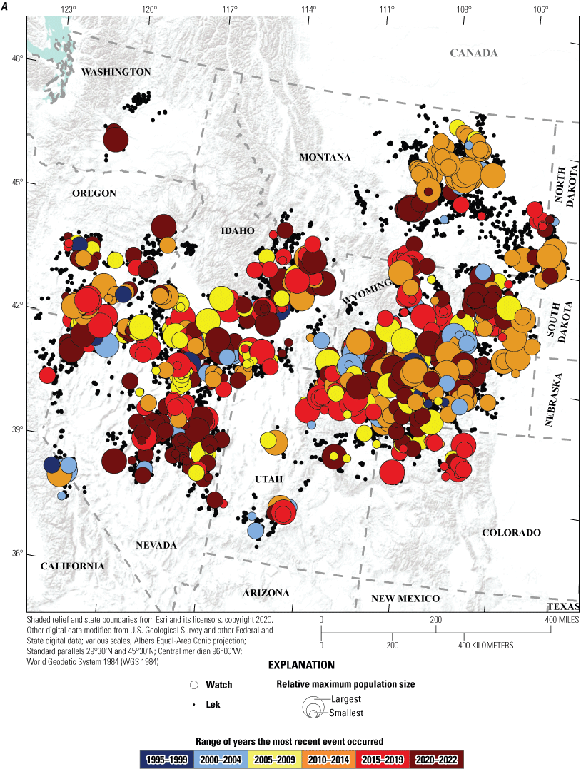

Spatial and temporal depiction of range-wide A, watches; and B, warnings of greater sage-grouse (Centrocercus urophasianus) population declines at the lek scale in the western United States from 1990 to 2022. Map image is the intellectual property of Esri and is used herein under license. Copyright© 2020 Esri and its licensors. All rights reserved.
We estimated 0.573 and 0.420 proportion of NCs were activated as first watches and warnings (table 3; fig. 6), respectively, at NCs range-wide during 1990–2022. An average of 0.018 (repeat=0.049) and 0.013 (repeat=0.040) proportion of clusters activated per year, which was approximately 7.6 (repeat=20.8) and 5.6 (repeat=16.8) clusters. We reported CC-A (Bi-State area) had the greatest proportion (1.000) of watches, whereas CC-E (Great Basin area) had the greatest number (first=170 and repeat=509) of watches across the 33-year timeframe. For warnings, CC-A had the greatest proportion (0.778; table 3) and CC-E had the greatest number (first=118 and repeat=376).
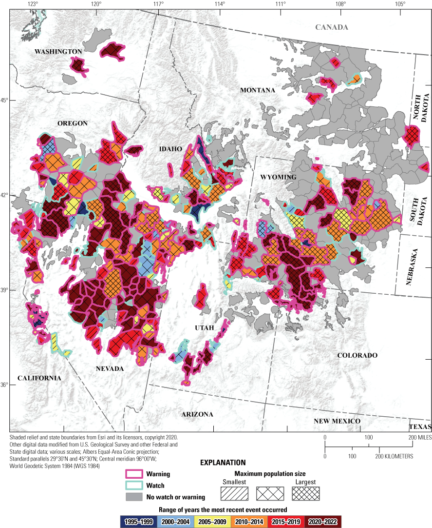
Spatial and temporal depiction of range-wide watches and warnings of greater sage-grouse (Centrocercus urophasianus) population declines at the neighborhood cluster scale in the western United States from 1990 to 2022. Map image is the intellectual property of Esri and is used herein under license. Copyright © 2020 Esri and its licensors. All rights reserved.
During 2022, we estimated 0.014 and 0.014 proportion of leks experienced first watches and warnings, respectively, range-wide (table 4), which resulted in 65 (repeat=418) and 67 (repeat=521) lek activations. During 2022, the greatest proportion of first watches (0.026) and warnings (0.029) were within CC-D and CC-F, respectively, which were 43 (repeat=127) watches and 27 (repeat=193) warnings (table 4). Climate cluster B had no lek-level watches activated during 2022, but it did have three repeat warnings (table 4). We estimated 0.000 and 0.014 proportion of neighborhoods experienced first watches and warnings, respectively, range-wide in 2022 (table 4). Climate cluster A experienced the greatest proportion of NC warnings (0.111) during 2022 followed by CC-F (0.019) and CC-E (0.018). Warnings and watches for each neighborhood cluster are available in Coates and others (2023).
Table 4.
Watches and warnings identified at the lek and neighborhood cluster (NC) scales across different climate clusters (A–F) by state-space model estimates using a targeted annual warning system framework for greater sage-grouse (Centrocercus urophasianus) across their range in the western United States during 2022. Number of watches and warnings that include repeat (r), only first time (f), and proportion (p) of populations (lek or NC) are reported.[Number of watches and warnings that include repeat (r), only first time (f), and proportion (p) of populations (lek or NC) are reported. Abbreviations: CC, climate cluster; A, Bi-State area; B, Washington area; C, Jackson Hole, Wyoming area; D, eastern area; E, Great Basin area; F, western Wyoming area]
References Cited
Bureau of Land Management, 2015, Notice of availability of the record of decision and approved resource management plan amendments for the Great Basin Region greater sage-grouse sub-regions of Idaho and southwestern Montana; Nevada and northeastern California; Oregon; and Utah—Department of the Interior, Bureau of Land Management: Federal Register, v. 80, p. 57633–57635, accessed August 15, 2022, at https://www.federalregister.gov/documents/2015/09/24/2015-24213/notice-of-availability-of-the-record-of-decision-and-approved-resource-management-plan-amendm.
Carlisle, J.D., Keinath, D.A., Albeke, S.E., and Chalfoun, A.D., 2018, Identifying holes in the greater sage-grouse conservation umbrella: The Journal of Wildlife Management, v. 82, no. 5, p. 948–957. [Available at https://doi.org/10.1002/jwmg.21460.]
Coates, P.S., Prochazka, B.G., O’Donnell, M.S., Aldridge, C.L., Edmunds, D.R., Monroe, A.P., Ricca, M.A., Wann, G.T., Hanser, S.E., Wiechman, L.A., and Chenaille, M.P., 2021, Range-wide greater sage-grouse hierarchical monitoring framework—Implications for defining population boundaries, trend estimation, and a targeted annual warning system: U.S. Geological Survey Open-File Report 2020–1154, 243 p., accessed August 15, 2022, at https://doi.org/10.3133/ofr20201154.
Coates, P.S., Prochazka, B.G., Aldridge, C.L., O’Donnell, M.S., Edmunds, D.R., Monroe, A.P., Hanser, S.E., Wiechman, L.A., and Chenaille, M.P., 2022a, Range-wide population trend analysis for greater sage-grouse (Centrocercus urophasianus)—Updated 1960–2022: U.S. Geological Survey Data Report 1165, 16 p., accessed March 20, 2022, at https://doi.org/10.3133/dr1165.
Coates, P.S., Prochazka, B.G., Aldridge, C.L., O’Donnell, M.S., Edmunds, D.R., Monroe, A.P., Hanser, S.E., Wiechman, L.A., and Chenaille, M.P., 2022b, Trends and a targeted annual warning system for greater sage-grouse in the western United States (1960–2021): U.S. Geological Survey data release, available at https://doi.org/10.5066/P9OQWGIV.
Coates, P.S., Prochazka, B.G., Aldridge, C.L., O'Donnell, M.S., Edmunds, D.R., Monroe, A.P., Hanser, S.E., Wiechman, L.A., and Chenaille, M.P., 2023, Trends and a targeted annual warning system for greater sage-grouse in the western United States (ver. 2.0, May 2023): U.S. Geological Survey data release, https://doi.org/10.5066/P9OQWGIV.
Connelly, J.W., Knick, S.T., Schroeder, M.A., and Stiver, S.J., 2004, Conservation assessment of greater sage-grouse and sagebrush habitats: Cheyenne, Wyo., Western Association of Fish and Wildlife Agencies, 611 p., accessed August 15, 2022, at https://wdfw.wa.gov/sites/default/files/publications/01118/wdfw01118.pdf.
Dinkins, J.B., Lawson, K.J., and Beck, J.L., 2021, Influence of environmental change, harvest exposure, and human disturbance on population trends of greater sage-grouse: PLoS One, v. 16, no. 9, p. e0257198. [Available at https://doi.org/10.1371/journal.pone.0257198.]
Doherty, K.E., Evans, J.S., Coates, P.S., Juliusson, L.M., and Fedy, B.C., 2016, Importance of regional variation in conservation planning—A rangewide example of the greater sage-grouse: Ecosphere, v. 7, no. 10, p. 1–27, accessed August 15, 2022, at https://doi.org/10.1002/ecs2.1462.
Garton, E.O., Connelly, J.W., Horne, J.S., Hagen, C.A., Moser, A., and Schroeder, M., 2011, Greater sage-grouse population dynamics and probability of persistence, in Knick, S.T., and Connelly, J.W., eds., Greater sage-grouse—Ecology and conservation of a landscape species and its habitats: Berkeley, Calif., University of California Press, Studies in Avian Biology, v. 38, p. 292–381, accessed August 15, 2022, at https://doi.org/10.1525/california/9780520267114.003.0016.
Hanser, S.E., and Knick, S.T., 2011, Greater sage-grouse as an umbrella species for shrubland passerine birds—A multiscale assessment, in Knick, S.T., and Connelly, J.W., eds., Greater sage-grouse—Ecology and conservation of a landscape species and its habitats: Berkeley, Calif., University of California Press, Studies in Avian Biology, v. 38, p. 474–487, accessed August 15, 2022, at https://doi.org/10.1525/california/9780520267114.003.0020.
Miller, R.F., Knick, S.T., Pyke, D.A., Meinke, C.W., Hanser, S.E., Wisdom, M.J., and Hild, A.L., 2011, Characteristics of sagebrush habitats and limitations to long-term conservation, in Knick, S.T., and Connelly, J.W., eds., Greater sage-grouse—Ecology and conservation of a landscape species and its habitats: Berkeley, Calif., University of California Press, Studies in Avian Biology, v. 38, p. 144–184, accessed August 15, 2022, at https://doi.org/10.1525/california/9780520267114.003.0011.
O’Donnell, M.S., Edmunds, D.R., Aldridge, C.L., Heinrichs, J.A., Monroe, A.P., Coates, P.S., Prochazka, B.G., Hanser, S.E., Wiechman, L.A., Christiansen, T.J., Cook, A.A., Espinosa, S.P., Foster, L.J., Griffin, K.A., Kolar, J.L., Miller, K.S., Moser, A.M., Remington, T.E., Runia, T.J., Schreiber, L.A., Schroeder, M.A., Stiver, S.J., Whitford, N.I., and Wightman, C.S., 2021, Synthesizing and analyzing long-term monitoring data—A greater sage-grouse case study: Ecological Informatics, v. 63, p. 101327. [Available at https://doi.org/10.1016/j.ecoinf.2021.101327.]
Rich, T.D., Wisdom, M.J., and Saab, V.A., 2005, Conservation of sagebrush steppe birds in the interior Columbia Basin, General Technical Report PSW-GTR-191, in Ralph, C.J., Rich, T., and Long, L., eds., Proceedings of the third international partners in flight conference: Albany, Calif., U.S. Department of Agriculture, Forest Service, Pacific Southwest Research Station, p. 589–606.
Rowland, M.M., Wisdom, M.J., Suring, L.H., and Meinke, C.W., 2006, Greater sage-grouse as an umbrella species for sagebrush-associated vertebrates: Biological Conservation, v. 129, no. 3, p. 323–335, accessed August 15, 2022, at https://doi.org/10.1016/j.biocon.2005.10.048.
Schroeder, M.A., Aldridge, C.L., Apa, A.D., Bohne, J.R., Braun, C.E., Bunnell, S.D., Connelly, J.W., Deibert, P.A., Gardner, S.C., Hilliard, M.A., Kobriger, G.D., McAdam, S.M., McCarthy, C.W., McCarthy, J.J., Mitchell, D.L., Rickerson, E.V., and Stiver, S.J., 2004, Distribution of sage-grouse in North America: The Condor, v. 106, no. 2, p. 363–376, accessed August 15, 2022, at https://doi.org/10.1093/condor/106.2.363.
U.S. Department of Agriculture Forest Service, 2015a, Notice of availability of the record of decision and approved land management plan amendments for the Great Basin Region greater sage-grouse sub-regions of Idaho and southwestern Montana; Nevada and Utah: Federal Register, v. 80, p. 57333–57334, accessed August 15, 2022, at https://www.federalregister.gov/documents/2015/09/23/2015-24169/notice-of-availability-of-the-record-of-decision-and-approved-land-management-plan-amendments.
U.S. Department of Agriculture Forest Service, 2015b, Notice of availability of the record of decision and approved land management plan amendments for the Rocky Mountain Region greater sage-grouse sub-regions northwest Colorado and Wyoming: Federal Register, v. 80, p. 57332–57333, accessed August 15, 2022, at https://www.federalregister.gov/documents/2015/09/23/2015-24169/notice-of-availability-of-the-record-of-decision-and-approved-land-management-plan-amendments.
U.S. Fish and Wildlife Service, 2015, Endangered and threatened wildlife and plants; 12-month finding on a petition to list greater sage-grouse (Centrocercus urophasianus) as an endangered or threatened species: Federal Register, v. 80, no. 191, p. 59857–59942, accessed August 15, 2022, at https://www.govinfo.gov/content/pkg/FR-2015-10-02/pdf/2015-24292.pdf.
Western Association of Fish and Wildlife Agencies, 2015, Greater sage-grouse population trends—An analysis of lek count databases 1965–2015: Cheyenne, Wyo., Western Association of Fish and Wildlife Agencies, 55 p., accessed August 15, 2022, at https://ir.library.oregonstate.edu/concern/technical_reports/ng451p621.
Datum
Vertical coordinate information is referenced to the North American Vertical Datum of 1988 (NAVD 88).
Horizontal coordinate information is referenced to the World Geodetic System (WGS 84).
Elevation, as used in this report, refers to distance above the vertical datum.
Abbreviations
estimated abundance
estimated intrinsic rate of population change
estimated finite rate of population change
BLM
Bureau of Land Management
CC
climate cluster
CRI
credible interval
MCMC
Markov chain Monte Carlo
N
abundance
NC
neighborhood cluster
QA/QC
quality assessment and quality control
SSM
state-space model
USGS
U.S. Geological Survey
WAFWA
Western Association of Fish and Wildlife Agencies
For more information concerning the research in this report, contact the
Director, Western Ecological Research Center
U.S. Geological Survey
3020 State University Drive East
Sacramento, California 95819
https://www.usgs.gov/centers/werc
Publishing support provided by the U.S. Geological Survey
Science Publishing Network, Sacramento Publishing Service Center
Suggested Citation
Coates, P.S., Prochazka, B.G., Aldridge, C.L., O'Donnell, M.S., Edmunds, D.R., Monroe, A.P., Hanser, S.E., Wiechman, L.A., and Chenaille, M.P., 2023, Range-wide population trend analysis for greater sage-grouse (Centrocercus urophasianus)—Updated 1960–2022: U.S. Geological Survey Data Report 1175, 17 p., https://doi.org/10.3133/dr1175.
ISSN: 2771-9448 (online)
Study Area
| Publication type | Report |
|---|---|
| Publication Subtype | USGS Numbered Series |
| Title | Range-wide population trend analysis for greater sage-grouse (Centrocercus urophasianus)—Updated 1960–2022 |
| Series title | Data Report |
| Series number | 1175 |
| DOI | 10.3133/dr1175 |
| Year Published | 2023 |
| Language | English |
| Publisher | U.S. Geological Survey |
| Publisher location | Reston, VA |
| Contributing office(s) | Western Ecological Research Center |
| Description | Report: viii, 17 p.; Data Release |
| Country | United States |
| Online Only (Y/N) | Y |
| Google Analytic Metrics | Metrics page |