

Chandeleur Islands to Breton Island Bathymetric and Topographic Datasets and Operational Sediment Budget Development: Methodology and Analysis Report
Links
- Document: Report (47.8 MB pdf) , HTML , XML
- Download citation as: RIS | Dublin Core
Acknowledgments
This study is part of the Coastal Protection and Restoration Authority (CPRA) Barrier Island Comprehensive Monitoring (BICM) program (carried out under CPRA contract number 2000339324, BICM2–Chandeleurs TopoBathy DEM). The authors thank project managers Darin Lee and Dr. Syed Khalil for their collaboration on this study and, along with Glen Curol (CPRA), their valuable review of the report. The authors acknowledge the U.S. Geological Survey (USGS) field teams for years of data collection and processing, Betsy Boynton for assistance with the graphics, Stephen Bosse for format assistance, USGS scientists David Thompson and Joseph Terrano, and editor Stokely Klasovsky for their valuable review.
Introduction
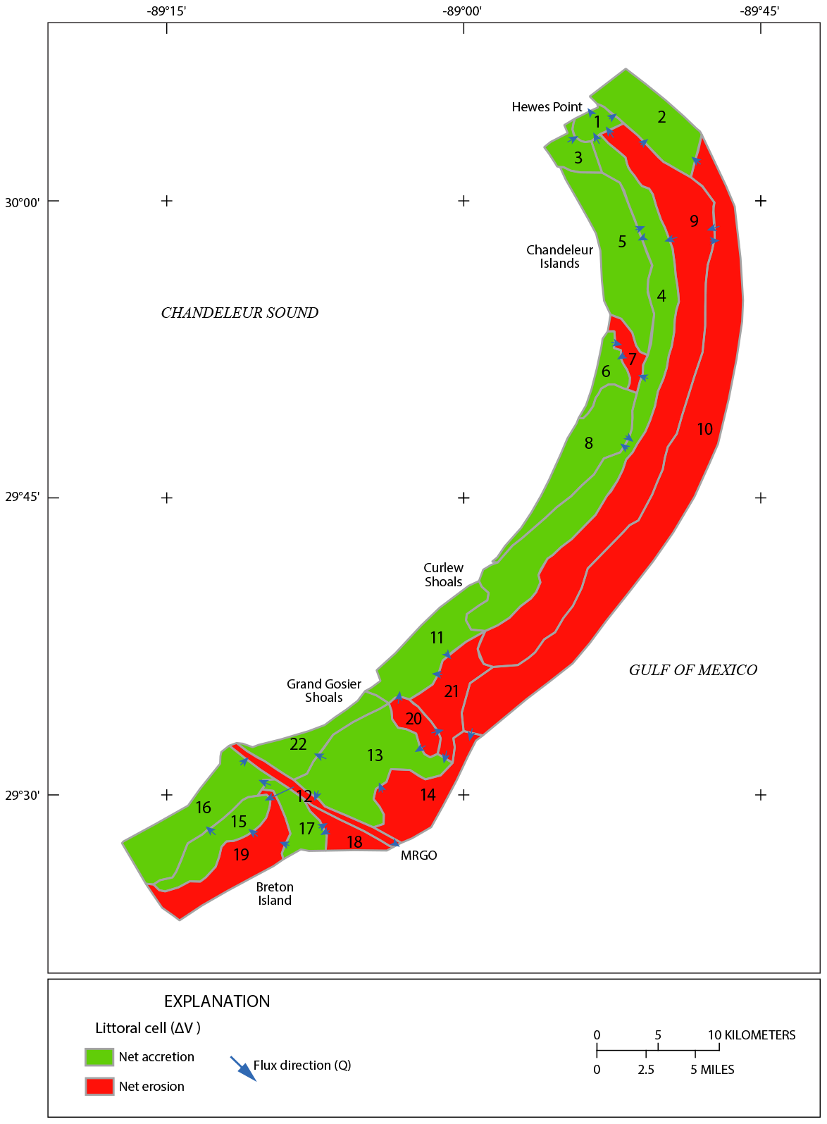
The Chandeleur Islands, Louisiana (La.), and Breton Island, La., barrier island arc, which includes Curlew and Grand Gosier Shoals, is located in the Breton National Wildlife Refuge (BNWR) within the northern Gulf of Mexico (fig. 1). Created in 1904, the Refuge covers the coastal waters east of the Mississippi River Delta and provides protected habitat for endangered species such as pelicans, terns, and sea turtles (U.S. Fish and Wildlife Service [USFWS], 2008). The islands support some of the only sea-grass beds in Louisiana (Poirrer, 2007; Poirrer and Handley, 2007), provide wave protection for the mainland of the Mississippi River Delta (FitzGerald and others, 2016), and regulate the balance of freshwater from the river with saltwater from the Gulf of Mexico (Reyes and others, 2005). This balance provides nursery habitat for many commercially and recreationally important fishes (USFWS, 2008).
The former Curlew and Grand Gosier Islands—now ephemeral shoals—and Breton Island comprise the southern extent of the barrier arc (fig. 1). The Chandeleur Islands formed through the transgressive evolution (Penland and others, 1988) of the St. Bernard delta complex of the Mississippi River, which was abandoned between 2,000 and 1,800 years ago through avulsion to a more favorable gradient through present day southern Louisiana (Frazier, 1967; Rogers and others, 2009). As the abandoned delta lobe submerged, waves reworked sandy distributary-channel sediments into a sandy shoal-tidal inlet system that migrated with the rising sea level. Over time, vertical development and the amalgamation of the shoals led to subaerial extension and the formation of barrier islands. As the increasing elevation reduced tidal influence, wave-dominated processes formed beach ridges and overwash deposits that were stabilized by colonizing marsh vegetation (Penland and others, 1988). Due to its isolated position and alignment with an earlier delta-lobe progradation (Frazier, 1967; Rogers and others, 2009), it is possible that Breton Island formed under similar circumstances but predates the Chandeleur Islands to the north.
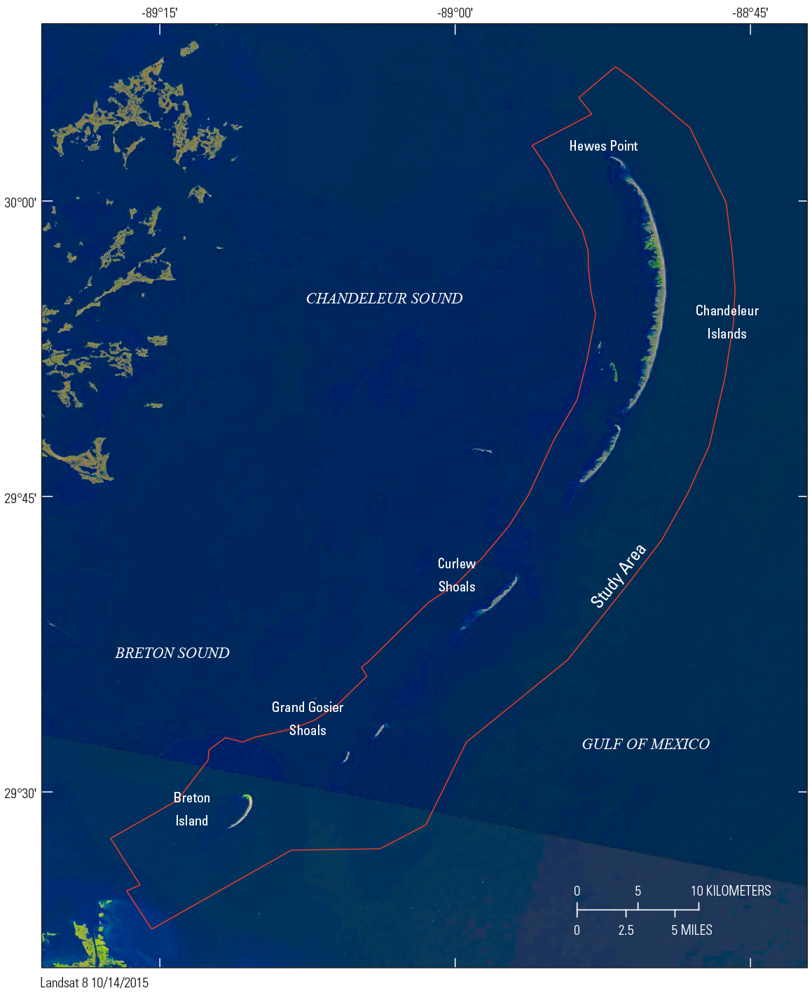
U.S. Geological Survey Landsat 8 imagery showing the Chandeleur Islands, Louisiana (La.), Curlew and Grand Gosier Shoals, and Breton Island, La., located within the Breton National Wildlife Refuge. Topographic and bathymetric study area is shown by red outline.
The modern barrier system is composed of deltaic, marine, and barrier island deposits. The submerged island platform supporting the Chandeleur and Breton Islands is composed of 85 percent very fine sand (Flocks and others, 2009a; Flocks and Terrano, 2016) with tidal inlets and overwash deposits that consist of approximately 75 percent very fine sand. The back-barrier environment (Chandeleur and Breton Sounds) is composed primarily of silt deposits, with up to 52 percent sand (Flocks and others, 2009a). Shell lags occur throughout the system, having concentrated during high-energy events such as storms. The prevailing wave climate from the Gulf of Mexico is from the southeast (Ellis and Stone, 2006), resulting in bidirectional littoral sand transport away from the center of the Chandeleur barrier island system to flanking depositional centers (Ellis and Stone, 2006; Georgiou and Schindler, 2009; Miner and others, 2009a). Deposits at Hewes Point, the terminal spit at the northern end of the Chandeleur Islands (fig. 1), have a higher sand content (97 percent) than the rest of the island platform, and the sand is slightly coarser-grained and better sorted than other barrier-platform sediments (Flocks and others, 2009a). Through the interpretation of geophysical profiles and sediment cores collected across Hewes Point, it is estimated that the deposit may contain up to 340×106 cubic meters (m3) of sand (Flocks and others, 2009b).
The Chandeleur Islands are in a constant state of change due to natural processes such as land subsidence, sea-level rise, sediment transport, and hurricane impacts. Geologic processes no longer contribute new sediment for island growth; as a result, the islands experience extreme rates of land loss (Lavoie, 2009). Direct observation and computer modeling indicate that the islands could be reduced to shoals over the next decade (Fearnley and others, 2009), thereby losing the ability to support critical habitat. The rates of shoreline change within the Chandeleur Islands are some of the highest in Louisiana; the average rate of change from the late 1800s to 2015 is 9.5 meters per year (m/yr) (Byrnes and others, 2018) or three times the average rate of shoreline change for the State. This rate accelerated from 6.7 m/yr at the turn of the 19th century to 114.5 m/yr at the turn of the 21st century (Byrnes and others, 2018) as the islands collapsed from a nearly continuous island arc with high dunes to segmented, low-elevation islets.
The Chandeleur Islands have been the focus of intense study by the U.S. Geological Survey (USGS), in collaboration with the Louisiana Coastal Protection and Restoration Authority (CPRA) and the USFWS. Scientists documented island characteristics and change through remote sensing, sediment sampling, and computer modeling (Lavoie, 2009; Kindinger and others, 2013) and examined island response to numerous hurricane impacts (Fearnley and others, 2009; Sallenger and others, 2009) as well as human alteration through the construction of the Deepwater Horizon oil spill mitigation sand berm (Plant and others, 2014; Miselis and others, 2015). These studies couple short-term observations with long-term geologic characterizations, assess barrier island change over multiple time scales, and develop predictive scenarios for the island's fate. This information is critical for helping resource managers respond to environmental and human-made challenges.
This study is part of the CPRA Louisiana Barrier Island Comprehensive Monitoring (BICM) program. The goal of the BICM program is to provide long-term data on the barrier islands of Louisiana for monitoring change and assisting in coastal management. The BICM program uses historical data and acquires new data to map and monitor shoreline position, sediment properties, topography, bathymetry, and habitat. Since 2006, the USGS has collected geophysical and sedimentologic data across the BNWR through the BICM program and collaborative USGS projects such as the Barrier Island Evolution Research project (https://www.usgs.gov/centers/spcmsc/science/barrier-island-evolution; under CPRA contract number 2000339324, BICM2–Chandeleurs TopoBathy DEM), which builds upon the previous BICM physical assessment of the BNWR outlined in Kindinger and others (2013). This project uses topographic and bathymetric data from three periods (1917–1922, 2006–2007, and 2013–2015) to develop digital elevation models (DEMs), measure elevation change, and calculate sediment budgets for the barrier island system. The sediment budget analysis, derived from the volumetric change between the three periods, is necessary for understanding sediment transport dynamics along barrier islands and providing information for effective coastal management. This report describes the methods used to acquire, process, and produce these products.
Data Sources
1920s Bathymetry Data
The bathymetric data representing the 1920s are from a collection of lead-line measurements. At each sounding, the survey vessel stopped—in shallow water, a lead weight was lowered and raised by hand; in deeper waters (greater than 28 m), the weight was raised by either a steam or electric motor (National Centers for Environmental Information [NCEI], 1922a). It should be noted that boat movements and currents can move the line during the measurement and increase errors in the sounding depth. The geographic position was determined by using a sextant to sight three fixed points, all of which were either marker buoys or land-based controls (NCEI, 1922a). The soundings were transcribed onto hydrographic sheets (H-sheets) later digitized and archived by the National Oceanic and Atmospheric Administration (NOAA) National Centers for Environmental Information.
Figure 2 shows an H-sheet used in this study. The digitized data are available for download as American Standard Code for Information Interchange (ASCII) data files that contain the H-sheet number, latitude, longitude, and water depth from the NOAA Bathymetric Data Viewer (https://www.ncei.noaa.gov/maps/bathymetry/). A description of the methods used to acquire the data can be found in the survey reports (for example, NCEI [1922b]) provided online with the datasets. Additional information, such as acquisition and digitizing dates, horizontal and vertical datums, and sampling methods are also available as metadata files for each H-sheet. In this study, five H-sheets were used to cover the Chandeleur-Breton nearshore area (table 1). The footprint of the H-sheets extends 75 kilometers (km) into the Gulf of Mexico and 35 km north into Mississippi Sound (fig. 3).
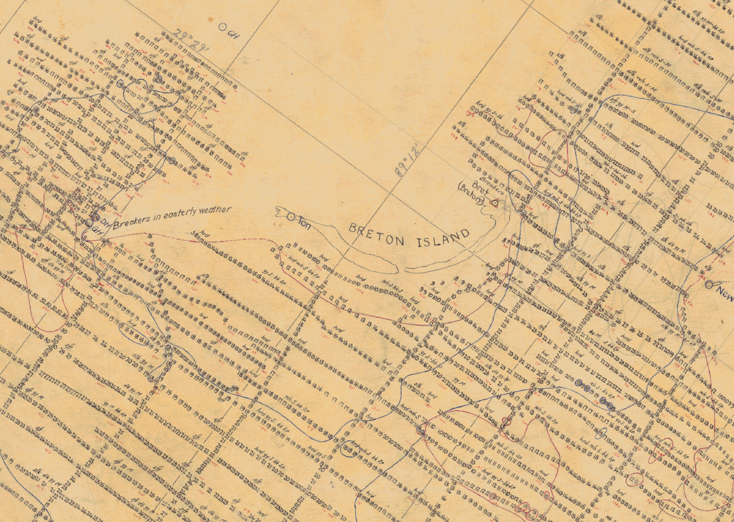
Digitally scanned image of a hydrographic sheet (Register Number 4223; National Centers for Environmental Information, [NCEI], 1922c) created in 1922 by the U.S. Coast and Geodetic Survey that includes the waters around Breton Island, Louisiana. Water-depth values are in feet at mean low water. Georeferenced water-depth values are available as digital data files through the National Oceanic and Atmospheric Administration’s National Centers for Environmental Information (https://www.ncei.noaa.gov).
Additional sources were used to supplement gaps in the bathymetric point coverage. The shorelines from the Chandeleur Islands to Breton Island were digitized from 1922 U.S. Coast and Geodetic Survey (USCGS) topographic maps (T-sheets) (USCGS, 1922a, b, c, d) by Martinez and others (2009) to produce Esri1 shapefiles. For this study, the shoreline vectors were reduced to points, and each point was assigned an elevation of +0.25 meter (m) referenced to the orthometric height in the North American Vertical Datum of 1988 (NAVD 88). This elevation is a nominal height above sea level to assist in resolving the shoreline in grid generation and is used in other elevation studies in the Gulf of Mexico (for example, Buster and Morton [2011]).
Esri refers to the Esri company’s associated ArcGIS software products.
The same T-sheets display tidally submerged areas that contain both tidal flats and salt marshes. A study by Fagherazzi and others (2006) found that tidal areas have bimodal elevations of around −0.5 m for tidal flats, and +0.25 m for salt marshes. No distinction is made between tidal flats and salt marshes in this study; these areas were digitized and assigned a median elevation of +0.0 m (NAVD 88), representing mean sea level (fig. 4). Along the Chandeleur Sound side of the southern Chandeleur Islands and Breton Island, shallow areas were not mapped during the 1922 survey. These areas were augmented with depth measurements acquired in 1898 (fig. 3) and digitized from the 1915 reissue of USCGS hydrographic chart number 192 (USCGS, 1899; table 1). Only areas that showed significant data gaps were supplemented with 1898 data points.
Table 1.
Hydrographic maps, topographic maps, and other data sources used to generate the 1920 digital elevation model used in this study.[La., Louisiana; m, meter; NAD 83, North American Datum of 1983; NAVD 88, North American Vertical Datum of 1988; NCEI, National Centers for Environmental Information; T-sheet, topographic map; USCGS, U.S. Coast and Geodetic Survey; UTM16N, Universal Transverse Mercator zone 16 north]
| Source map or survey | Source citation | Survey location and date | Elevation range (m NAVD 88) |
Geographic range (m NAD 83, UTM16N) |
|---|---|---|---|---|
| H–04000 | NCEI, 1918 | Northern Chandeleur Islands, La., 1917 | −4.72 to −0.07 | 287258/328175 3312533/3363596 |
| H–04171 | NCEI, 1921 | Northern Chandeleur Islands, La., 1920 | −12.50 to −1.07 | 322129/406815 3288216/3344811 |
| H–04212 | NCEI, 1922a | Gulf of Mexico, 1922 | −17.22 to −1.33 | 307426/382353 3257722/3320581 |
| H–04219 | NCEI, 1922b | Chandeleur Sound, 1922 | −2.18 to −0.04 | 296392/322245 3285729/3314997 |
| H–04223 | NCEI, 1922c | Southern Chandeleur Islands, La.; Breton Island, La., 1922 | –26.05 to −0.46 | 272353/349264 3221639/3287566 |
| 1T-sheet 3918 | USCGS, 1922b | Shorelines, Chandeleur Islands, La., to Breton Island, La., 1922 | +0.25 | 283988/324876 3260880/3326345 |
| 1,2T-sheets 3917–3920 | USCGS, 1922a–d | Tidal zone, Chandeleur Islands, La., to Breton Island, La., 1922 | +0.00 | 283960/324900 3260844/3326473 |
| 3Hydrographic chart 192 | USCGS, 1899 | Chandeleur Sound, 1898 | −5.20 to −0.32 | 280888/323621 3258523/3312122 |
Data from Martinez and others (2009) were used in conjunction with these sources. A +0.25 m elevation is used to assist in resolving the shoreline during gridding.
Only points covering areas that showed significant data gaps were used. See figure 3 for locations.
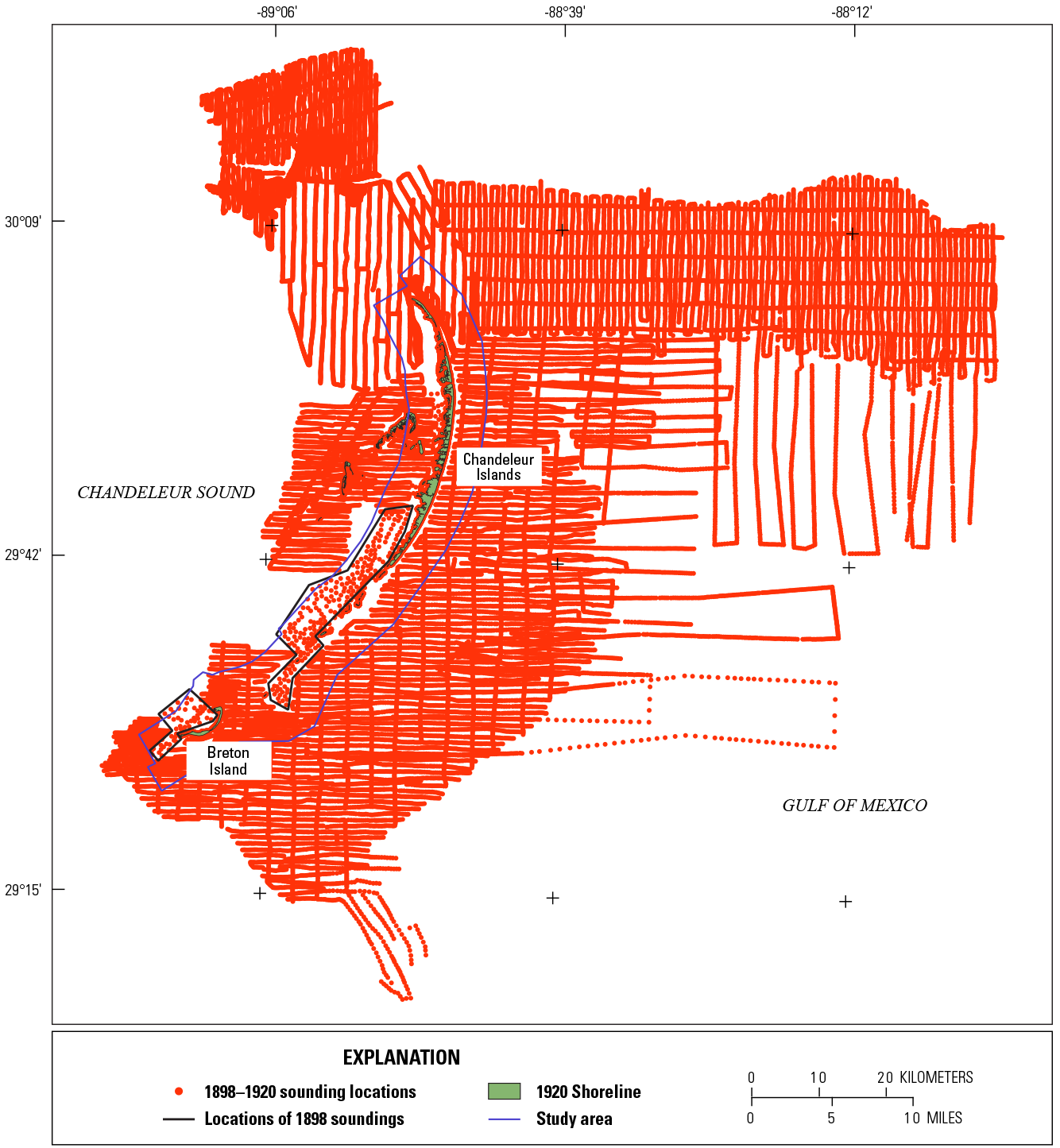
Map of the Chandeleur Islands and Breton Island, Louisiana, showing the data points used to generate the 1920s digital elevation model, shoreline position, and area of study. The study area is shown by the blue outline. Areas supplemented with soundings from the 1898 survey (U.S. Coast and Geodetic Survey [USCGS], 1899) are enclosed by black polygons.
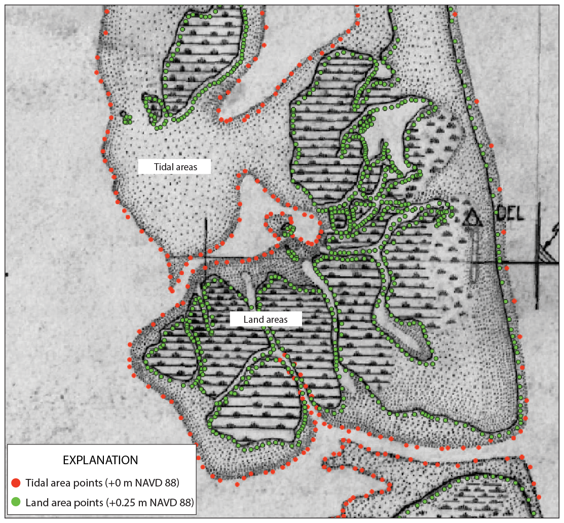
Image of the georectified 1922 topographic map (T-sheet) (Shalowitz, 1962). Elevation values of +0.25 meter (m) (North American Vertical Datum of 1988 [NAVD 88]) and 0.0 m (NAVD 88) were interpolated for land areas and tidal areas, respectively.
The 1920s hydrographic data are horizontally referenced to the North American Datum of 1927 (NAD 27) relative to mean low water (MLW). Water depths were measured in feet and converted to meters for archiving. For this study, all datasets were converted horizontally to the North American Datum of 1983 (NAD 83) reference frame and NAVD 88 using the National Geodetic Survey (NGS) geoid model 12B (GEOID12B). Geographic coordinates were converted to the projected Universal Transverse Mercator (UTM) zone 16 north coordinate reference system (table 2). These geospatial transformations were performed using NOAA VDatum (ver. 3.9; https://vdatum.noaa.gov/) software. The conversions allowed for the direct comparison of elevations between periods to determine the elevation change and calculate volumetric change. The file formatting for the resulting data files is described in appendix 1.
Table 2.
Example input-output conversions of data points from H-sheet 04223 (National Centers for Environmental Information [NCEI], 1922c).[GEOID12B, geoid model 12B; m, meter; MLW, mean low water, NA, not applicable; NAD 27, North American Datum of 1927; NAD 83, North American Datum of 1983; NAVD 88, North American Vertical Datum of 1988; TSS, topography of the sea surface; UTM, Universal Transverse Mercator]
2006–2007 Bathymetry Data
As part of the BICM program, single-beam and interferometric-swath acoustic bathymetry data were collected from Hewes Point to Breton Island during the summers of 2006 and 2007. The surveys extended from the shoreline to approximately 7 km offshore on the Gulf of Mexico side and approximately 5 km on the Chandeleur and Breton Sound sides (fig. 5). The single-beam survey strategy included shore-perpendicular lines 1 km apart, and shore-parallel lines 1 km apart, out to a distance of 4 km. Offshore, full-swath coverage was obtained to a distance of 7 km. For detailed information on the data collection, processing, and reporting of the 2006–2007 BICM surveys, see Miner and others (2009a, 2009b) and Baldwin and others (2009).
The Chandeleur Island and Breton Island shorelines were derived from a combination of digital orthophoto quarter quadrangles (DOQQs) and DigitalGlobe QuickBird satellite imagery (Martinez and others, 2009; Miner and others, 2009b) and represent the shoreline configuration in 2005, shortly after Hurricane Katrina reduced the island area by over 60 percent from the previous year (Martinez and others, 2009). To augment the bathymetric data for DEM development, the vector shorelines were reduced to points and each point was assigned an elevation of +0.25 m (NAVD 88) to represent the subaerial shoreline; this nominal elevation is used to resolve the shoreline (Buster and Morton, 2011). The combined shoreline- and bathymetric-data file is projected horizontally to an NAD 83 reference frame and vertically to NAVD 88 using the GEOID12B model. The file formatting for the resulting data files is described in appendix 1.
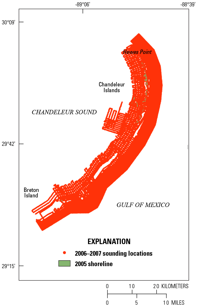
Map showing the data points used to generate the 2006–2007 digital elevation model and shoreline position.
2007 Topographic Light Detection and Ranging (Lidar) Data
Classified (attributed) 2007 bare-earth lidar data for the Chandeleur Islands, in LASer (LAS) file format, were obtained from Smith and others (2009), and detailed information about the lidar data acquisition and processing procedures can be found in that report. The classified LAS data were transformed from NAVD 88, geoid model 03 (GEOID03) to NAVD 88, GEOID12B to ensure consistency among all topographic datasets. The classified LAS files were reprojected and transformed using VDatum (ver. 3.9) software.
Breton Island bare-earth topography data were not included in the Smith and others (2009) dataset. Classified 2007 bare earth lidar-derived elevation data for Breton Island, in LAS format, were obtained through the BICM program. The edited xyz lidar data were reprojected from NAD 83, UTM zone 15N, in meters, to NAD 83 (2011), UTM zone 16N, in meters. The xyz data were then converted to LAS (ver. 1.2) format using LAStools (ver. 181119) (https://rapidlasso.com/lastools/) software. An LAS clipping boundary for Breton Island was developed to extract the bare-earth LAS data for Breton Island. These data were combined with the bare-earth lidar data from the Chandeleur Islands to provide complete topographic coverage for the study area (fig. 6).
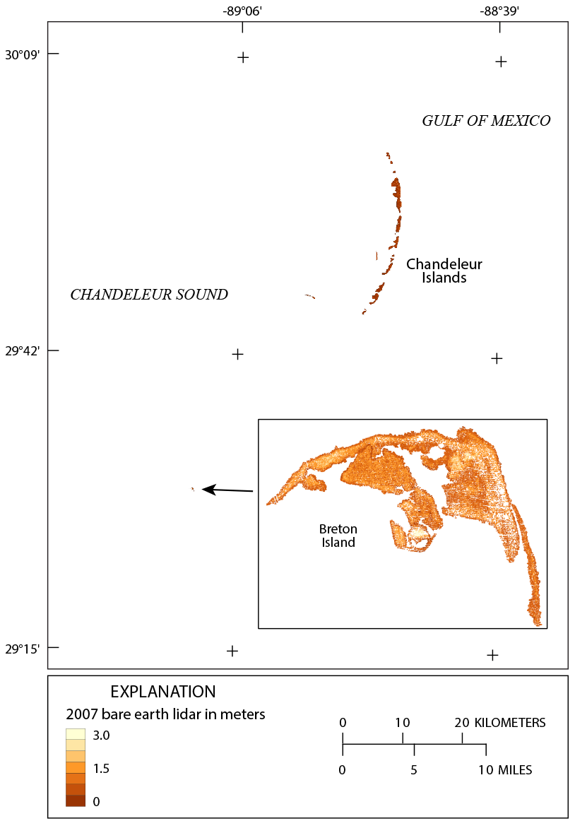
Map showing bare-earth topographic elevation data points from the 2007 light detection and ranging (lidar) surveys of the Chandeleur Islands and Breton Island, Louisiana. Only a small portion of Breton Island was emergent at this time. Curlew and Grand Gosier Shoals were submerged.
To reduce the point density within the combined topographic point cloud, a blockmean filter was applied to the data at a 1-m interval. The blockmean filter from Generic Mapping Tools (ver. 5) (https://www.soest.hawaii.edu/gmt/) software reads arbitrarily located xyz data and outputs a mean position and value at the designated interval. This method reduces coordinate samples below the Nyquist wavelength, which can produce spurious signals at larger wavelengths, to a representative constraining value (Smith and Wessel, 1990). The filter is applied prior to generating a surface. The file formatting for the resulting data files is described in appendix 1.
2013–2015 Bathymetry Data
Between 2013 and 2015, bathymetric surveys were conducted from the Chandeleur Islands to Breton Island through a coordinated effort between the BICM program and the USGS Barrier Island Evolution Research project. In July and August 2013, approximately 429 line-km of single-beam and interferometric-swath data were collected in the shallow waters around the northern Chandeleur Islands and Hewes Point (fig. 7). The study monitored the evolution of a sand berm constructed along the shoreline as part of the effort to mitigate the effects of the Deepwater Horizon oil spill (Lavoie and others, 2010). Survey tracklines extend north of the islands to include the borrow pit excavated to provide sand for the berm. For a detailed description of data acquisition, processing, and reporting, see DeWitt and others (2017).
In July and August 2014, the USGS conducted high-resolution geophysical and sedimentologic investigations around Breton Island to construct a comprehensive baseline assessment of the physical environment in preparation for the USFWS Natural Resource Damage Assessment Program restoration of the island. The investigation included single-beam and interferometric-swath bathymetry around Breton Island, extending approximately 10 km into the Gulf of Mexico and 5 km into Breton Sound (fig. 7). The bathymetric surveys also extended northeast to the Grand Gosier Shoals.
Approximately 2,500 line-km of bathymetric data were acquired, covering 356 square kilometers of seafloor. For a detailed description of data acquisition, processing, and reporting, see DeWitt and others (2016). As part of the BICM program, 1,613 line-km of single-beam bathymetric data were collected in June 2015, from the Grand Gosier Shoals to Hewes Point, to fill in areas not covered by earlier surveys (fig. 7). For this survey, shore-perpendicular line spacing was 500 m, with three shore-parallel lines collected at the shoreline, 1 km offshore of the shoreline, and 3 km offshore. For a detailed description of data acquisition, processing, and reporting, see Stalk and others (2017).
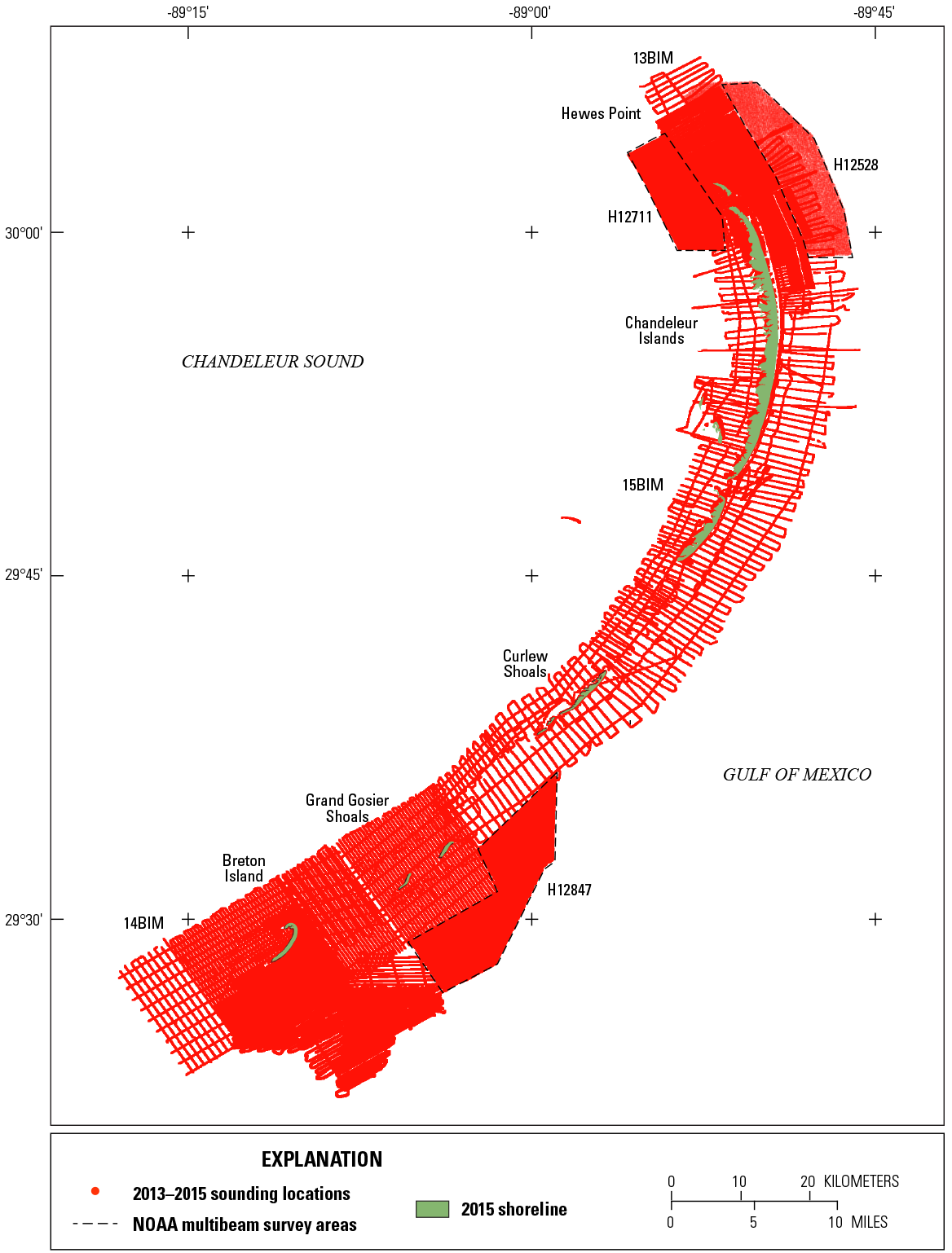
Map showing data points used to generate the 2013–2015 digital elevation model and shoreline position. Survey numbers on the map are found in table 3. NOAA, National Oceanic and Atmospheric Administration.
To supplement the bathymetric coverage, three hydrographic surveys contracted by NOAA were acquired from the NOAA Bathymetric Data Viewer (https://www.ncei.noaa.gov/maps/bathymetry/). These surveys were full, multibeam coverages conducted in 2013 (H12528 [NCEI, 2014]) and 2015 (H12711 [NCEI, 2015]) around Hewes Point and in 2015 (H12847 [NCEI, 2016]) offshore of Breton Island (table 3; fig. 7). To reduce the density of the point clouds within the NOAA multibeam surveys, a blockmean filter was applied to the data at a 10-m interval, as described in the previous section. To extend seafloor coverage to the island shorelines, data points along the 2015 shoreline were extracted from topographic lidar data acquired in February 2015. The 2015 topographic lidar dataset is discussed in the next section. All six datasets (table 3) were projected to the NAD 83, UTM16N, and NAVD 88 (GEOID12B) using VDatum (ver. 3.9) software. The file formatting for the resulting data files is described in appendix 1.
Table 3.
Bathymetric and light detection and ranging (lidar) data sources used to generate the 2013–2015 digital elevation model used in this study.[La., Louisiana; m, meter; NAVD 88, North American Vertical Datum of 1988; NAD 83, North American Datum of 1983; NCEI, National Centers for Environmental Information; UTM16N, Universal Transverse Mercator zone 16]
| Source map or survey | Source citation | Survey location and date | Elevation range (m NAVD 88) |
Geographic range (m NAD 83 UTM16N) |
|---|---|---|---|---|
| 13BIM1 | DeWitt and others, 2017 | Northern Chandeleur Islands, La., 2013 | −13.44 to −0.10 | 315463/329854 3305661/3327821 |
| 14BIM1 | DeWitt and others, 2016 | Breton Island, La., 2014 | −10.57 to −0.45 | 276852/304540 3251344/3276018 |
| 15BIM1 | Stalk and others, 2017 | Gosier Island, La., to Hewes Point, La., 2015 | −15.57 to 0.11 | 3270978/3333277 299332/329851 |
| H12711 | NCEI, 2015 | Hewes Point, La., to Chandeleur Sound, 2015 | −10.14 to −3.41 | 313308/320076 3318136/3326952 |
| H12528 | NCEI, 2014 | Hewes Point, La., to Gulf of Mexico, 2013 | −15.33 to −6.17 | 317124/329236 3317716/3331340 |
| H12847 | NCEI, 2016 | Breton Island, La., to Gulf of Mexico, 2015 | −10.27 to −3.62 | 297687/308101 3259703/3276619 |
| 2015 lidar2 | Digital Aerial Solutions, 2016 | Chandeleur Islands, La., to Breton Island, La., 2015 | 0.0 to +0.25 | 287734/324252 3261982/3324222 |
2015 Topographic Light Detection and Ranging (Lidar) Data
Bare-earth topographic lidar data were acquired from Hewes Point to Breton Island in February 2015. The survey was conducted for the USGS by Digital Aerial Solutions; for details on lidar data collection, processing, and quality assurance and quality control, see Digital Aerial Solutions (2016). The data are provided as tiled point clouds (1,500×1,500 m) classified by land-cover type, breaklines to support the hydroflattening of DEMs, intensity tiles, and bare-earth DEM tiles. The horizontal spatial reference is NAD 83, UTM zone 15N m, and the vertical datum is NAVD 88, geoid model 12A (GEOID12A). For the study area, 166 LAS tiles were downloaded and xyz values (processed and classified bare earth) were extracted and reprojected to NAVD 88, UTM zone 16N m, and NAVD 88, GEOID12B, using LAStools. The areas were clipped to island polygons using shoreline shapefiles extracted from the dataset breaklines (fig. 8). Due to the high density of the point clouds, the data points were reduced using the GMT blockmean filter at 1 m, as described in the “2007 Topographic Light Detection and Ranging (Lidar)” section.
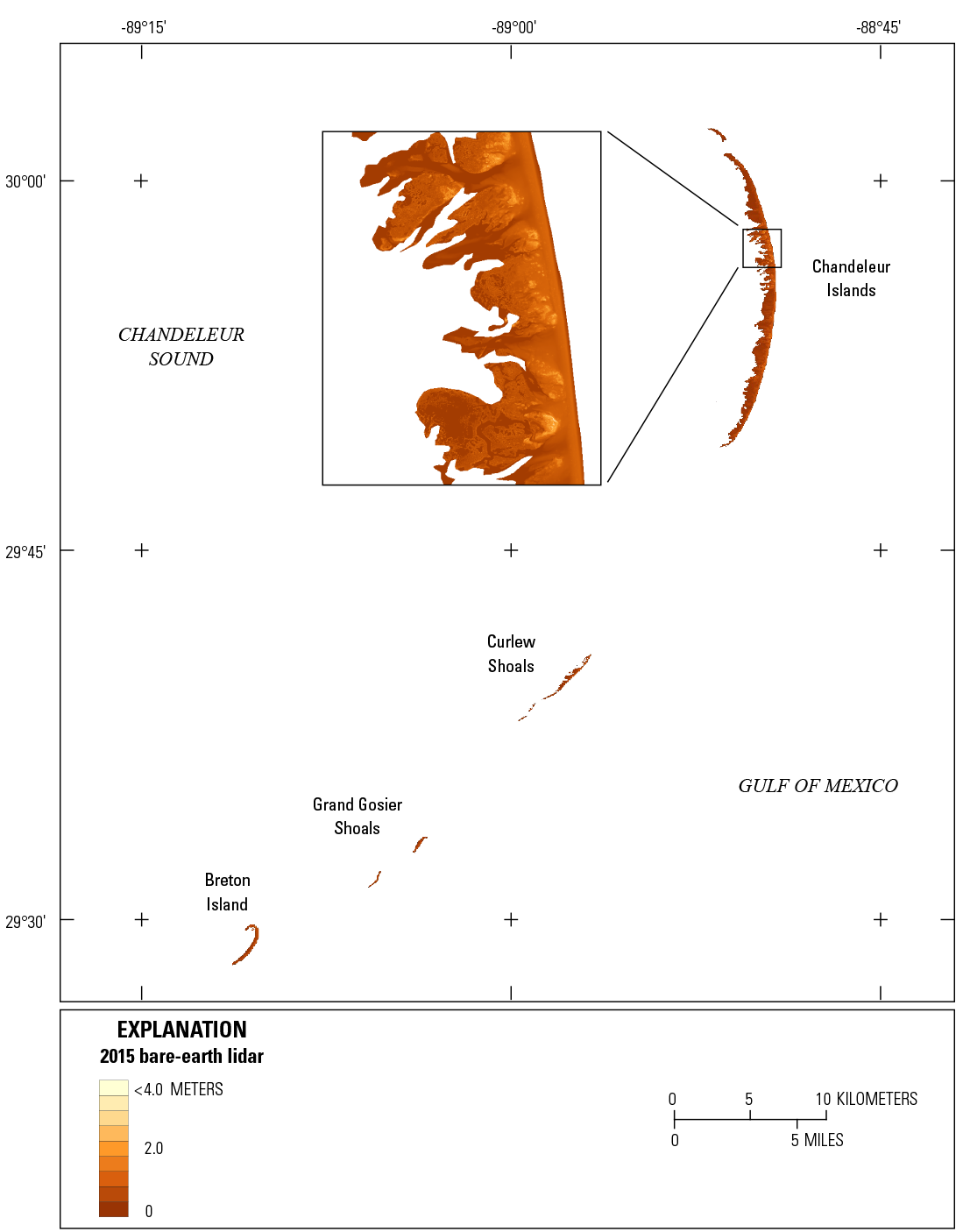
Map showing bare-earth topographic elevation data points from the 2015 light detection and ranging (lidar) survey of the Chandeleur Island barrier arc, Curlew and Grand Gosier Shoals, and Breton Island, Louisiana.
Deriving the Digital Elevation Models, Raster Map, and Contour Map
A DEM was derived separately for each topographic and bathymetric dataset, with the bathymetric DEMs shown in figures 9–11. The procedure used to generate the DEM and associated products is common across datasets through use of a series of processing steps in the Esri ArcGIS software:
-
Convert the ASCII-xyz point file from each dataset into an Esri shapefile.
-
Generate a triangulated irregular network (TIN) with elevation (z) as the height field using the “Create TIN” tool.
-
Clip the TIN to the study area spatial-extent polygon using the “hard clip” feature in the “Edit TIN” tool. The topographic TIN files generated from lidar datasets are further edited using breaklines as “hard clip” features to clear spurious features at the edges.
-
Generate a raster dataset using the “TIN to Raster” tool. The Nearest Neighbor interpolation method is used, with a cell size of 2.0 m for the lidar datasets and 50.0 m for the bathymetric datasets. The raster dataset is then exported to a raster image in the Tagged Image File Format (TIFF).
-
Generate a contour vector shapefile from the raster dataset using the “Contour” tool in ArcGIS with a contour interval of 1 m. The fields in the vector attribute table are populated according to the CPRA Coastal Information Management System (CIMS) attribute-labeling convention (Coastal Protection and Restoration Authority of Louisiana, 2016).
There are no elevation data available for the barrier islands in the historic (1922) dataset; all subaerial areas were set to the shoreline elevation of +0.25 m. For comparison with the historic dataset, the subaerial areas of the 2006–2007 and 2013–2015 datasets were also set to the shoreline elevation +0.25 m. An additional dataset was created for each of the 2006–2007 and 2013–2015 periods that included topographic lidar elevations for the subaerial areas so that the recent periods could be compared separately from the historical period, as described in the next section.
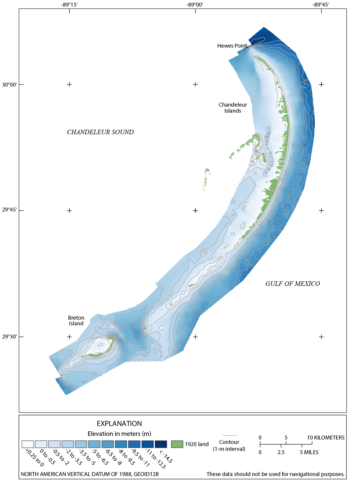
Digital elevation model generated from the 1898–1922 bathymetric and shoreline data. 1920 land is assigned an elevation of +0.25 meter North American Vertical Datum of 1988. GEOID12B, Geoid model 12B.

Digital elevation model generated from the 2006–2007 bathymetric and shoreline data. GEOID12B, Geoid model 12B; MRGO, Mississippi River to Gulf Outlet.
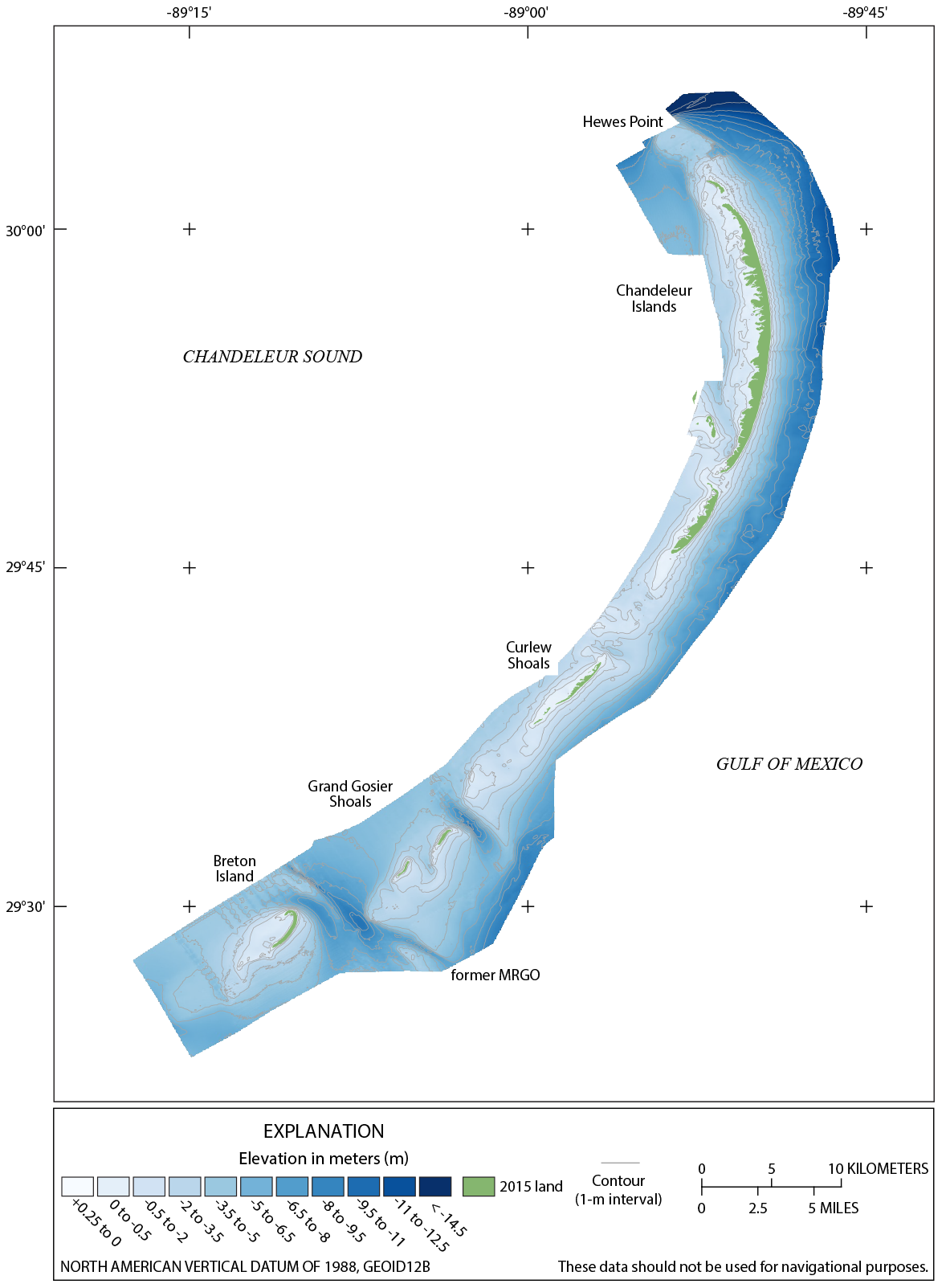
Digital elevation model generated from the 2013–2015 bathymetric and shoreline data. MRGO, Mississippi River to Gulf Outlet.
Merging Topographic and Bathymetric Datasets
Bare-earth lidar elevation data were integrated with bathymetric data as seamlessly as possible to accurately assess volumetric change between the 2006–2007 and 2013–2015 periods. The process provides a realistic transition across the shoreface where sediment transport processes are the most dynamic (Otvos, 1981) and is important for change assessment and hydrodynamic modeling. Topographic lidar and acoustic bathymetry are distinct elevation-acquisition techniques collected at separate spatial resolutions and during different periods and referenced to separate datums. There are often gaps in coverage between the shoreline derived from lidar and the water depth at which acoustic bathymetry can be feasibly recorded. As a result of these inconsistencies, there is inherent vertical uncertainty when merging the two datasets (Amante, 2018).
Merging the topographic-lidar data points with the bathymetric data points for both the 2006–2007 and 2013–2015 periods created an undesirable artifact in the resulting TIN and DEM. Figure 12 shows a two-dimensional profile extending across a part of the combined topographic-bathymetric DEM from onshore to offshore. In this example, two gridding methods were used to generate DEMs from the combined 2006 bathymetry and 2007 lidar topography. Both methods—a DEM generated from the TIN and a DEM generated using the kriging algorithm—resulted in a step pattern across the gap where the topographic and bathymetric data overlapped. This artifact is possibly a result of the lidar-derived shoreline data including surface-water areas (such as across inlets), differences in the point density of the lidar and bathymetric surveys, or a spatial gap between the lidar shoreline and the distance from shore at which bathymetric data were collected.
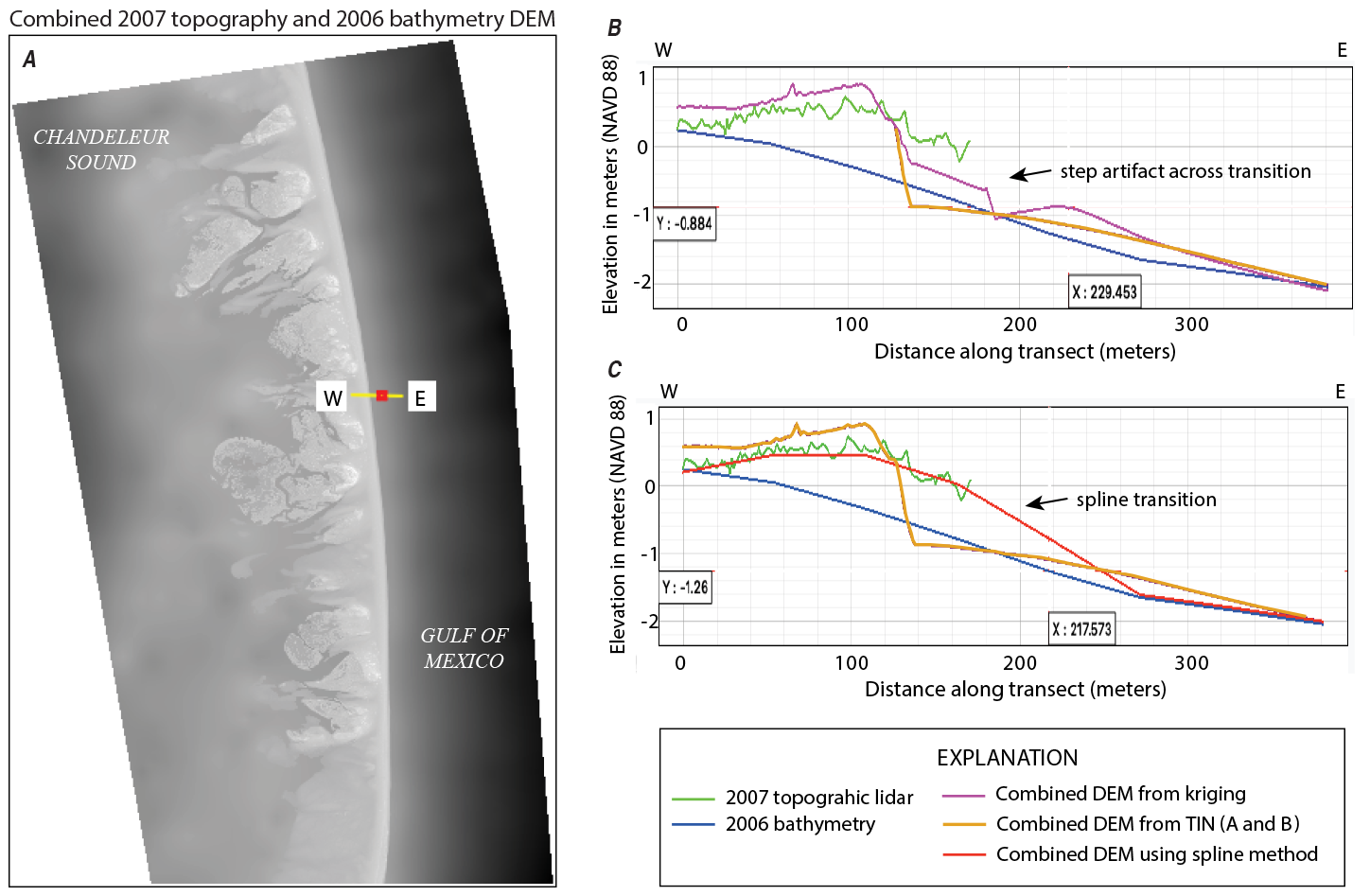
An image and two graphs that collectively show the step pattern that results from combining the 2006–2007 bathymetry and the 2007 light detection and ranging (lidar) topography and the process that mitigates that step pattern. A. Image showing the location of a west-to-east oriented profile (yellow line) across digital elevation models (DEMs) generated by combining 2006–2007 bathymetry with 2007 light detection and ranging (lidar) topography. B. The DEM elevation profiles were generated using the triangulated irregular network (TIN) method (orange line) and the kriging algorithm (purple line). Results show a step artifact across the transition from topography (green profile) to bathymetry (blue profile). C. Inserting additional data points across the transition using a spline interpolation process results in a more natural slope (red line). NAVD 88, North American Vertical Datum of 1988.
A series of processing steps—characterized in figure 13—was developed to generate a spline fit of interpolated data across the gap to better represent the natural physical slope of the shoreface. The steps involve sampling both the topographic and bathymetric data independently through the following process. The process was applied to both the 2006–2007 and 2013–2015 topobathymetric datasets prior to DEM development. Hereafter, “Sound” refers to the Breton and Chandeleur Sounds region of the study.
-
Establish vector line files that represent the Sound and Gulf shorelines (fig. 13A). For the 2006–2007 survey, the shoreline polygon of Martinez and others (2009) was used. For the 2013–2015 survey, the shoreline derived from the 2015 topographic lidar survey by Digital Aerial Solutions (2016) was used.
-
Generate two vector lines offset from either side of the vector shoreline (fig. 13B). The distance from the shoreline is user-specified and should intersect real data from the topographic and bathymetric surveys. For example, the offset line seaward of the Gulf shoreline should extend to a distance where it intersects bathymetric-survey tracklines. For this study, landward and seaward distances of 25 m and 100 m were selected, respectively (fig. 13B).
-
Generate points along the vector lines (fig. 13C). For this study, points were generated every 50 m using the “Points along lines” tool in the QGIS (ver. 3.6) software, and spatial geometry attributes were added to each point.
-
At each georectified point, sample elevation values from the topographic lidar (using the 25-m landward offset vector) and bathymetric (using the 100-m seaward offset vector) DEMs. Inspect the points and delete those that do not capture elevation values (for example, where the landward vector crosses an inlet).
-
Merge the landward- and seaward-sampled points into a single point file. For this study, the landward-seaward pair for the Gulf side was merged separately from the landward-seaward pair for the Sound side.
-
Using a spline algorithm, generate grids from the datasets (fig. 13D). For this study, the “v.surf.bspline” tool in QGIS (ver. 3.6) was used, with a spline length of 10 m, 1000 maximum iterations, and a cell size of 25 m.
-
Generate a spatially distributed array of points within the resulting grids. This is done using the “generate points (pixel centroid) within polygon” tool in QGIS (ver. 3.6). In this report, a polygon created from the seaward Sound and Gulf offset vectors was used as the clip polygon. Apply spatial attributes to the generated points.
-
At each georectified point, sample elevation values from the spline grids created in step 6. Each point should now have geometry and elevation attributes (xyz). Export the points as ASCII point values.
-
Merge the spline dataset created in step 8 with the bathymetric and topographic xyz data files.
-
Create TINs, raster DEMs, and contour vectors from the point files, as outlined earlier in this report, using ArcGIS.
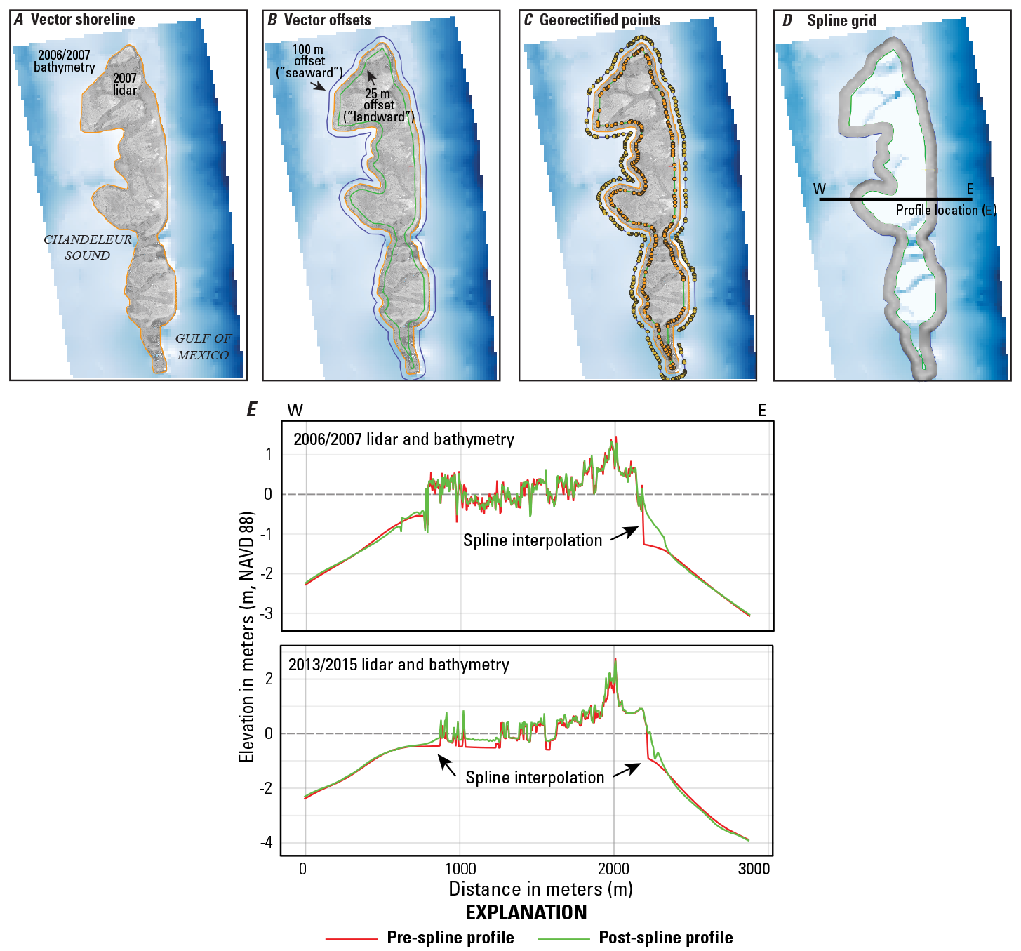
Images (A–D) and graph (E) showing the processing steps used to add interpolated points across the topographic to bathymetric transition using a spline method, which result in a more natural representation of the transition in the resulting digital elevation model (DEM). A. Example DEMs of the 2006–2007 bathymetry and the 2007 light detection and ranging (lidar) topography, with the shoreline delineated (orange line). B. Two vector lines offset from the shoreline—offset 25 meters (m) onto the topographic DEM and 100 m onto the bathymetric DEM. C. Generation of points along the offset vectors. These points are used to sample elevations from the underlying DEMs and create endpoints for the spline interpolation. D. The resulting spline grid. From this grid, a distribution of points is extracted and included with the merged topographic-bathymetric dataset for triangulated irregular network development. E. Profiles across the pre-spline DEM (top) and post-spline DEM (bottom) for the two periods. Location of profiles shown in D. Added spline interpolation shown by arrows. NAVD 88, North American Vertical Datum of 1988.
Using the above procedure, the two-dimensional profile shown in figure 12B (red line) shows the resulting, more natural representation of the land-to-sea transition across the shoreface. The resulting merged, topobathymetric DEMs for the 2006–2007 and 2013–2015 periods are shown in figure 14.
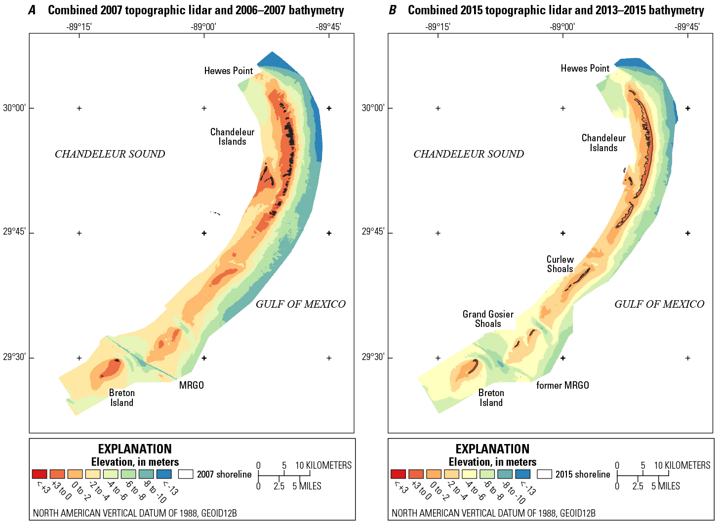
Topobathymetric digital elevation model for the (A) 2006–2007 and (B) 2013–2015 periods created by combining the topographic light detection and ranging (lidar), bathymetric, and spline interpolated data points. MRGO, Mississippi River to Gulf Outlet; GEOID12B, geoid model 12B.
Elevation and Volumetric Change Analyses
To simplify the following explanation on how the elevation change products were derived, the 1920s period is herein be referred to as 1920, the 2006–2007 period as 2007, and the 2013–2015 period as 2015. The DEMs were differenced using the ArcGIS “Minus” tool to quantify the change in elevation over the two periods (1920–2007 and 2007–2015). By subtracting the cell values of the earlier period from the later period, the product represents erosion if the cell value is negative and accretion if the cell value is positive. Due to errors associated with the topobathymetric data processing and DEM generation, any change within ±0.25 m is considered within the error and, therefore, is treated as no change. Since there are no subaerial elevations for the 1920 dataset, the elevation change model was derived from the 1920–2007 bathymetric DEMs. The 2007–2015 period used the topobathymetric DEMs described earlier.
1920–2007 Period Elevation and Volumetric Change Determination
During acquisition, the 1920 bathymetric data were referenced in MLW (NCEI, 1922c). In order to measure the elevation change between 1920 and 2007, as a result of sediment accretion or erosion, the MLW elevations must be adjusted to account for relative sea-level rise (RSLR), which is a combination of land subsidence and global sea-level rise. The RSLR must be factored out of the elevation change calculations so that only accretion and erosion are estimated in the volumetric change of an area. The rate of land subsidence at the Chandeleur and Breton Islands can be measured using Global Positioning Systems (GPSs) repeatedly stationed over fixed positions across long time intervals, such as days or months. The GPS base station measures elevation with high precision, which, when repeated over years, can measure elevation change rates on order with natural land subsidence.
The fixed positions are established benchmarks installed on the islands. On the Chandeleur Islands, the benchmark “MARK” was regularly occupied since its installation in 2001 (fig. 15). The USGS repeatedly occupied this benchmark from 2000 to 2017, supporting various surveys (for example, bathymetry, lidar, and ground control) for the islands. A GPS base station with a secured tripod was set upon the benchmark point (fig. 15). A high precision GPS receiver programmed in static mode, using a choker ring antenna to decrease multipath signals, was set to record at specified intervals (such as 1 second [s], 5 s, 30 s) respective to the survey parameters. The GPS base station was serviced twice daily, resulting in one day session and one night session per 24 hours. The base station, once erected, remained on the benchmark for the duration of the survey, which ranged from 1 day to >7 days. See the data acquisition section in DeWitt and others (2017) for more information on this method. Comparison of the repeat elevation measurements, recorded in ellipsoid height (International Terrestrial Reference Frame of 2000 [ITRF00]) over 16 years, produces a trendline with a land subsidence rate of 7 millimeters per year (mm/yr) (fig. 15A). This rate is used in the calculation of RSLR.
In addition to land subsidence, sea level has risen dramatically since 1920 (NOAA, 2017). Long-term tide gauges in the Gulf of Mexico measured sea-level trends ranging from +2.13 mm/yr (Florida peninsula) to +9.65 mm/yr (southern Louisiana). This variability is a function of land subsidence at the gauge location. The tide gauge at Pensacola, Florida, is considered most reflective of global sea-level rise since the area is tectonically stable with no measurable land subsidence (Buster and Morton, 2011). Sea-level trends at the Pensacola tide gauge show an average of +2.40 mm/yr since records began (fig. 15E). This sea-level rise rate, when added to the subsidence rate measured at the Chandeleur Islands, produces an RSLR of +9.4 mm/yr. This rate compares well with water-level trends measured at Grand Isle, La. (+9.08 mm/yr), and Eugene Island, La. (+9.65 mm/yr), which include a significant subsidence component (NOAA, 2017). Projected over the 87-year period between 1920 and 2007, a static shift of −0.82 m was applied to the 1920s bathymetric data to account for RSLR prior to differencing the 1920 and 2007 DEMs.
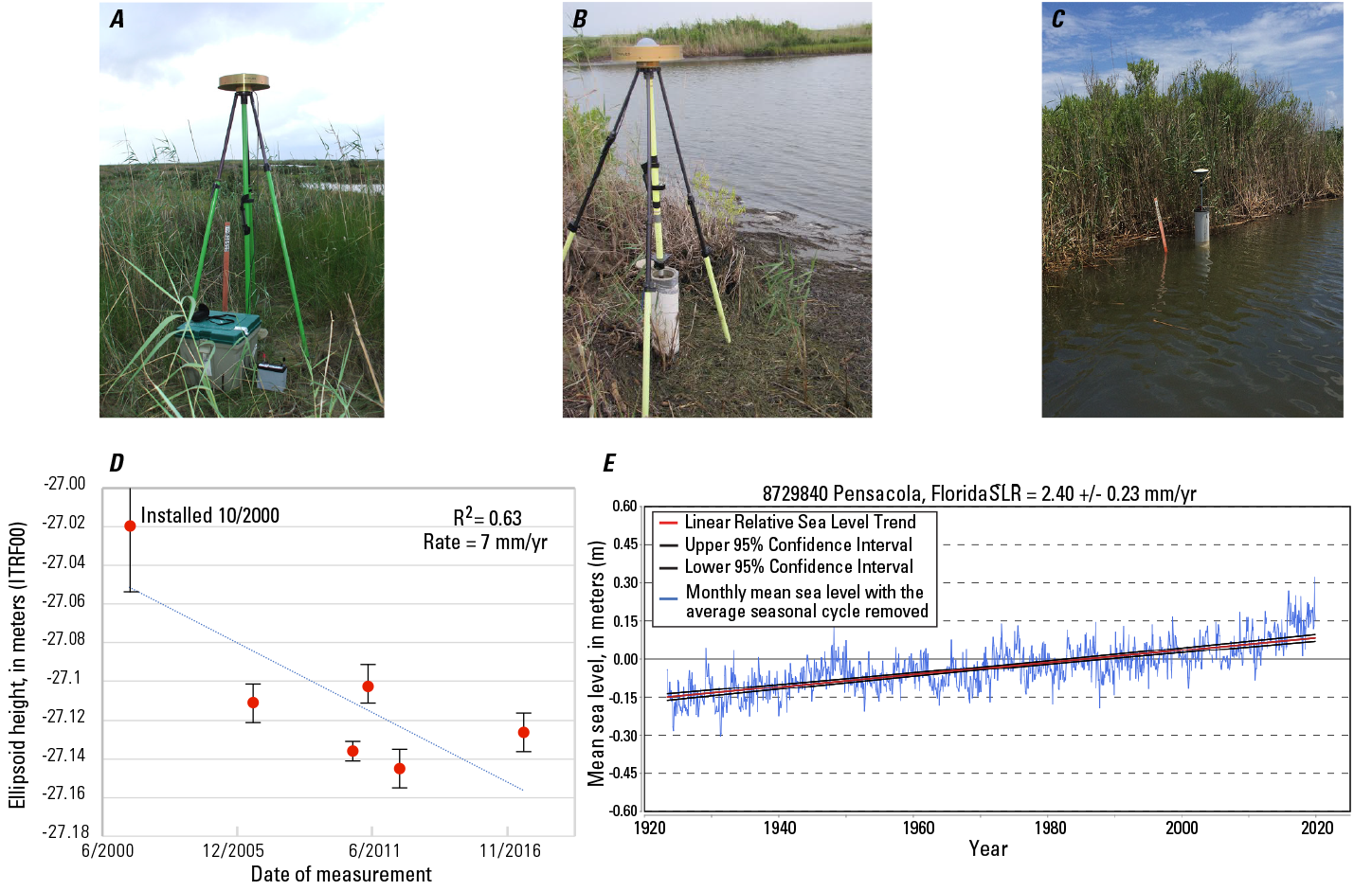
Photographs (A–C) and graphs (D–E) showing repeat occupation of the benchmark “MARK” installed at the Chandeleur Islands, Louisiana, and data from the tide gauge at Pensacola, Florida, providing an estimate of land subsidence over time. The photographs show the installed benchmark location in (A) 2006, (B) 2012, and (C) 2017. The photographs show the drastic effect of the combined land subsidence and land erosion of the islands between 2006 and 2017, with the benchmark casing first becoming exposed and then submerged. D. Linear regression plot (R2 is the goodness of fit for linear regression) of benchmark elevation measurements between 2000 and 2017 that provides a subsidence rate estimate of approximately 7 millimeters per year (mm/yr). E. Linear regression of water-level measurements over a 100-year period at the tide gauge (station ID 8728940) at Pensacola, Florida, provides a sea-level rise (SLR) of 2.4 mm/yr. Together, these estimates provide a relative sea-level rise (RSLR) rate of +9.4 mm/yr. Tide information obtained from National Oceanic and Atmospheric Administration (NOAA, 2020). ITRF00, International Terrestrial Reference Frame of 2000; %, percent.
The 1920s soundings were acquired using the lead-line technique (see the “1920s Bathymetry Data” section for a description); beginning in the 1930s, bathymetric surveys relied on acoustic fathometer systems. These two techniques can lead to differences in the direct measurement of water depths. As the lead-line is lowered, currents or boat movement can offset the line from a vertical position. For the study area, it is not possible to compare contemporaneous lead-line soundings to fathometer soundings. One 1922 lead-line survey (chart register number H04212 [NCEI, 1922a]) did cross fathometer soundings collected in 1940 (chart register number H06552 [NCEI, 1940]) outside of the study area (fig. 16A) in 15–50 m water depth. Due to the water depth, it is possible that there is little change in seafloor elevation between the two periods (18 years). Using the “Distance Matrix” tool in QGIS (ver. 3.9), it was determined that 374 soundings from the 1922 survey were within 125 m of soundings from the 1940 survey (where the average distance between sounding pairs is 75 m).
Assuming no change in the water depth between surveys, these soundings can be considered close enough to each other for a direct comparison of elevations between the two sounding techniques (fig. 16B). The comparison of the 374 adjacent sounding pairs results in the lead-line technique producing a deeper water depth 77 percent of the time, by an average of −0.68 m, compared with 18 percent deeper soundings by the fathometer technique (the 2 techniques produced identical soundings 5 percent of the time). Assuming no change in the seafloor elevation between 1922 and 1940, this comparison would suggest that a majority of the time there is an overestimate of water depth using the lead-line technique when compared to the fathometer. However, if this overestimation is due to the lead-line reading being affected by current or boat movement, it must be assumed that this error propagates as water depth increases because of the length of the lead-line. The comparison above was made at an average water depth of 25 m (fig. 16B)—water depths within the study area are generally less than 14 m (fig. 9). Adding a static correction (specifically, adding 0.68 m to all lead-line soundings) to the 1920s data points in the study area would disproportionally alter the shallow water depths more significantly. Thus, a more robust comparison within the study area, and preferably a contemporaneous comparison between techniques, would be necessary to compensate for a possible overestimate of water depth in the 1920s survey through a relative (nonstatic) correction relative to water depth.
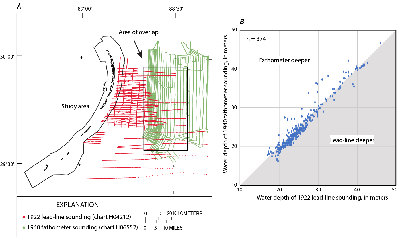
Images showing (A) location map of soundings proximate to the study area and (B) graph of sounding-depth comparisons. A. Location map shows overlapping 1920 lead-line soundings (red) and 1940 fathometer soundings (green) in an area approximately 21 kilometers from the study area. B. Sounding depth from the 1922 survey (National Centers for Environmental Information [NCEI], 1922a) compared with sounding depth from the 1940 survey (NCEI, 1940) when their horizontal positions are within 125 meters of each other. Assuming no change in water depth over the 18-year period between surveys, the soundings should be equal. The lead-line soundings were deeper (higher value) than the fathometer soundings 77 percent of the time.
The accretion-erosion map for the 1920–2007 period is shown in figure 17. Large amounts of elevation loss, or erosion, occur along the former 1920s subaerial footprint where the island migrated westward due to cross-shore and littoral sediment transport. The excavation of the MRGO ship channel is evident, as is the tidally driven incision of a channel between Grand Gosier and Curlew Shoals, removing up to 7 m of sediment (fig. 17). Depositional events include littoral accretion of sediment at Hewes Point (5–9 m) and the southern end of Grand Gosier Shoals (5 m).
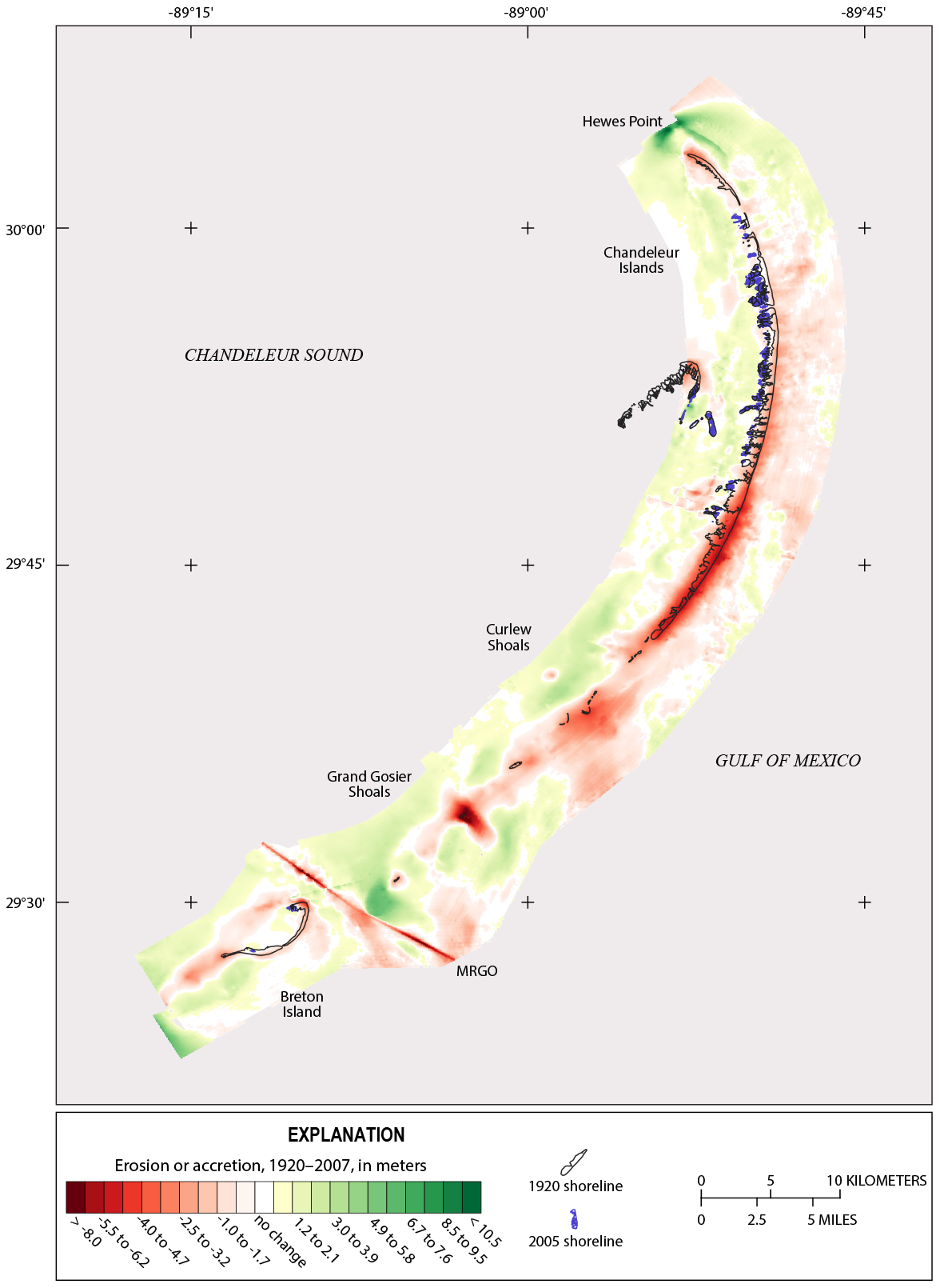
Elevation change map covering approximately 87 years. Change was determined by calculating the difference between the 1920 and 2007 bathymetric digital elevation models. The elevation change represents sediment accretion (positive values) and erosion (negative values) over this period. Elevation differences within ±0.25 meter and considered within error or “no change.” MRGO, Mississippi River to Gulf Outlet.
To characterize volumetric change, areas predominantly positive (accretion) or negative (erosion) in elevation change are identified and constrained by vector polygons (fig. 18). The spatial constraint provides the dimensionality to generate sediment volume. Positive and negative volumetric change within each polygon was calculated from the change raster map (fig. 17) using a series of commands within the GMT (ver. 5) suite of mapping tools. The process for quantifying volumetric change is as follows:
-
Extract individual polygons from the 1920–2007 difference map (GMT tools: “grdmask” with operators NAN/0/0; “grdmath–OR”).
-
For each polygon, separate into accretion (values less than +0.25 m set to NULL) and erosion (values greater than −0.25 m set to NULL) components (“grdmath–” GE, LE, MUL, and NAN).
-
Calculate area, volume, and maximum mean height (volume divided by area) for each polygon and output values to spreadsheet (“grdvolume”).
-
Calculate net volume change (accretion plus erosion) for each polygon. These values are reported in table 4.
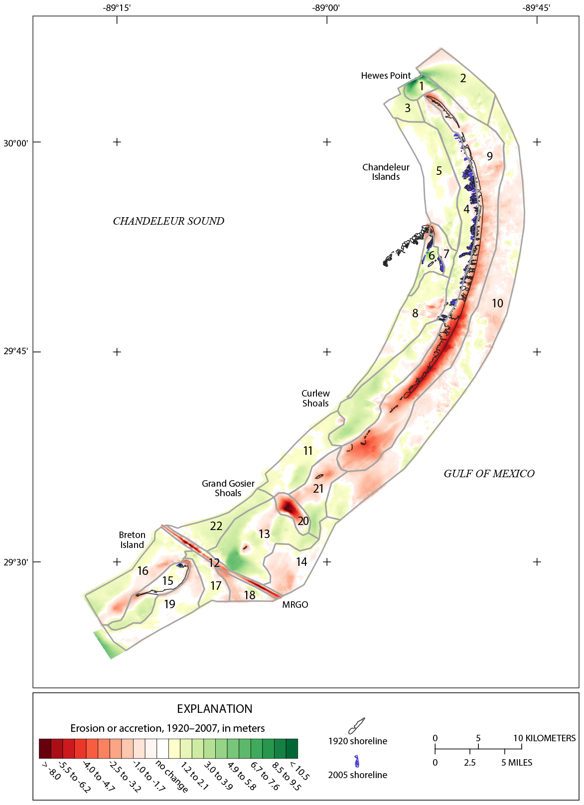
1920–2007 elevation change map with accretion-erosion areas identified by polygons. Numbers correspond to area statistics listed in table 4. MRGO, Mississippi River to Gulf Outlet.
Table 4.
Accretion-erosion statistics for each area outlined in figure 18. Error represents the volume within the range of uncertainty (±0.25 meter).[m, meter; m2, square meter; m3, cubic meter; NA, not applicable]
The accretion-erosion volume change statistics for the 1920–2007 period are shown in table 4. Net volumetric change ranged from 296×106 m3 of erosion along the axis of the 1920s subaerial footprint (fig. 18, polygon 9), to 73×106 square meters (m2) of accretion south of Gosier Shoals and along the Sound side of the island platform (fig. 18, polygons 13 and 4). The largest amount of sediment erosion per unit area occurred at the tidal channel between Curlew and Gosier Shoals (fig. 18, polygon 20), and the largest accretion per unit area occurred at Hewes Point (fig. 18, polygon 1). Across the study area, volumetric change between the 1920 and 2007 periods resulted in a net loss of 154×106 m3 of sediment from the system, most of that through the excavation of the MRGO, littoral sediment transport northward beyond Hewes Point, and the removal of sediment during major storms such as Hurricane Katrina.
Removal of Silt and Clay From the System
During high wave-energy events, sediment is mobilized into the water column and transported a distance relative to the amount and duration of current energy and the size and shape of the suspended sediment. Fine-grained material (silts and clays) remains in suspension longer, is transported greater distances, and can be removed from the system more readily than sand. The sediments that make up the Chandeleur Island platform and nearshore comprise a mixture of sands, silts, and clays. Flocks and others (2009a) analyzed the grain size of 106 sediment samples acquired from the top 1 m of sediment in 6- to 9-m water depth. They found that the sediments were composed of 72–84 percent very fine sand and 16–28 percent silts and clays. The silt and clay percentage can be used to calculate the fine-sediment load within the study area and determine the relative abundance of material that can be removed from the system.
For example, polygons 9 and 10 (fig. 18) correspond to the area of analysis for the sediment samples just described. The combined area of the two polygons is 293×106 m2 (table 4). The average vertical loss (erosion) within the polygons over the 1920–2007 period is −1.44 m, resulting in the removal of approximately 422×106 m3 of sediment. Using the percentage of silts and clays from above (16–28 percent), this corresponds to 68–118×106 m3 of fine-grained material removed. The net volume of all sediment removed from polygons 9 and 10 is 353×106 m3 (table 4); thus, 21–33 percent of all material removed can be accounted for through the loss of the silt and clay fraction.
2007–2015 Period Elevation and Volumetric Change Determination
Because the 1920s data had no topographic information, only the bathymetric change was calculated for the 1920–2007 period. Both the 2007 and 2015 periods included topographic lidar data, so the topobathymetric grids can be compared in this period. This is an important distinction in that land-elevation changes during the earlier period (such as dune loss) are not included, whereas during the later period the land-elevation change was captured.
Because the 2007 and 2015 elevations were orthometric—or referenced to a geoid model of the earth and not to sea-level—the comparison of the 2007 and 2015 topobathymetric DEMs did not require the static adjustments necessary for the earlier (1920–2007) period. The difference map for the 2007–2015 period is shown in figure 19. Most noticeable over this approximate 8-year period is the recovery of the island and shoals from the devastating erosion caused by Hurricane Katrina as sediment moved back onshore. This is evidenced by the expanding shoreline area in figure 19 in spite of landward translation and the continuing erosion on the Gulf-side shoreface. The borrow pit excavated to provide sand for the Deepwater Horizon oil spill mitigation sand berm is visible at Hewes Point (fig. 19), where approximately 3.5×10⁶ m2 of sediment was removed to construct the berm (Plant and others, 2014). Other elevation changes within the study area include a line of accretion along the MRGO (fig.19). After Hurricane Katrina, the MRGO ship channel was no longer maintained and subsequently infilled through natural-slope equilibration (Flocks and Terrano, 2016) by up to 4 m of sediment (fig. 20).
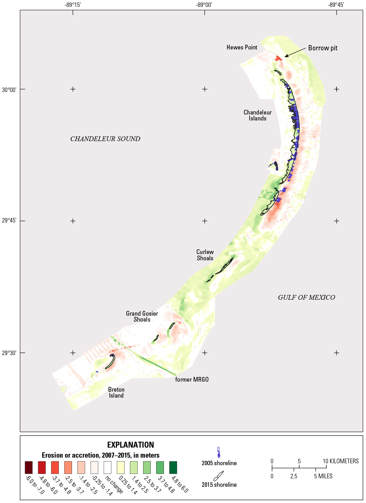
Elevation-change map covering approximately 8 years, as determined by calculating the difference between the 2007 and 2015 digital elevation model. The elevation change represents sediment accretion (positive values) and erosion (negative values) over the period. Elevation differences within ±0.25 meter are considered within error or “no change.” MRGO, Mississippi River to Gulf Outlet.
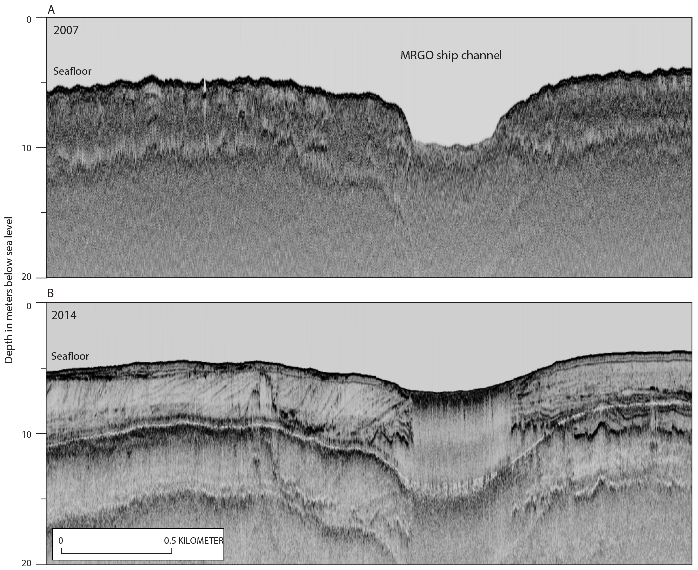
Seismic subbottom profiles from across the Mississippi River to Gulf Outlet (MRGO) ship channel (A) collected in 2007 (Baldwin and others, 2009), and (B) reoccupied in 2014 (Forde and others, 2016), that reflect the infilling of the channel after decommissioning and a cessation of maintenance dredging after Hurricane Katrina.
Areas predominantly positive (accretion) or negative (erosion) in elevation change are identified and constrained by vector polygons (fig. 21) to characterize volumetric change. Since the areas of change differ between periods, the polygons are different from those in the earlier period (fig. 18). The spatial constraint provides the dimensionality to generate volume. The positive and negative volumetric change within each polygon was calculated from the change raster using the previously described process; area and volume statistics are reported in table 5.
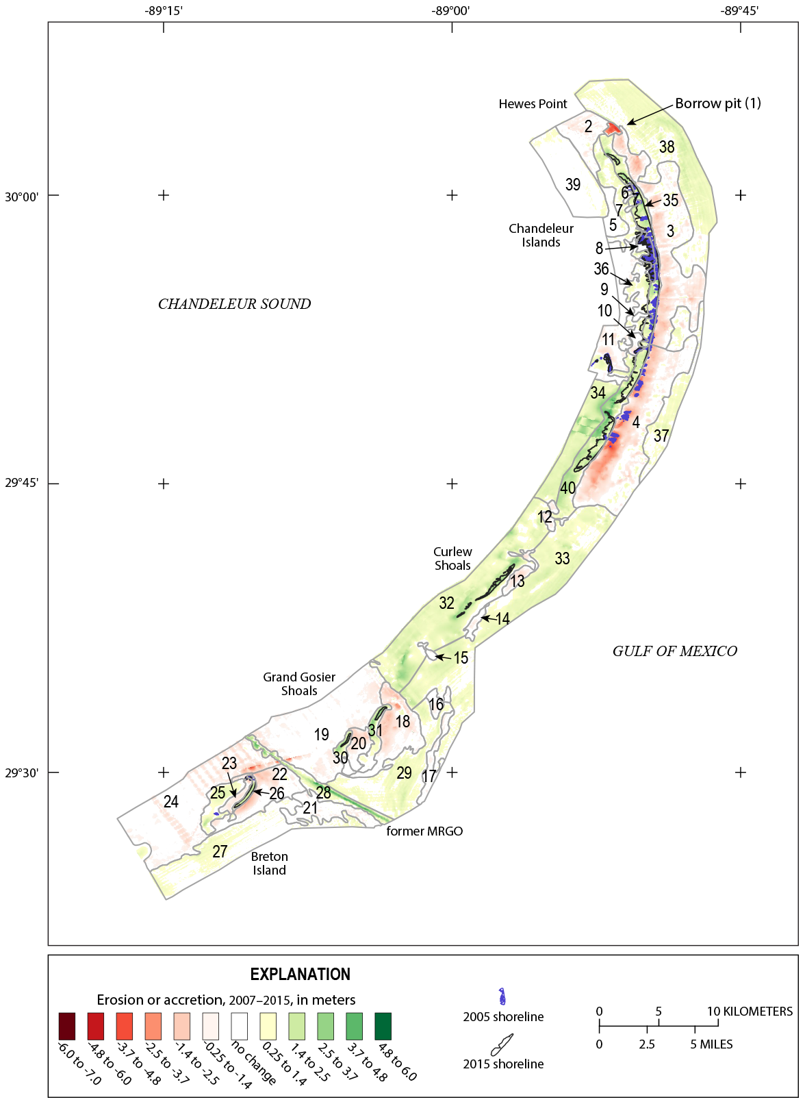
Elevation-change map for 2007–2015, with 40 accretion-erosion areas identified by polygons. Numbers correspond to the polygon numbers listed in the first column of table 5. MRGO, Mississippi River to Gulf Outlet.
Table 5.
Accretion-erosion statistics for numbered areas outlined in figure 21. Error represents the volume within the range of uncertainty (±0.25 meter).[m, meter; m3, cubic meter; NA, not applicable]
The 2007–2015 period experienced a net accretion of 101×106 m3 over the entire study area. This value indicates that the system (as delineated here) is not closed, and sediment is transported into the study area from both the Gulf and Sound sides of the islands. Sediment that eroded during Hurricane Katrina is returning to the island platform through nonstorm, wave-driven, onshore bar accretion. This type of process is documented for other coastal systems. Offshore of Fire Island, New York, Schwab and others (2017) observe that an onshore-directed sediment flux from the Inner Continental Shelf is required to balance the coastal sediment budget for Fire Island, and sediments on the Inner Continental Shelf are activated during storm events in waters as deep as 30 m. Other studies along the Atlantic coast show an open coastal system, with storm events moving a significant amount of sediment from the shoreface to the inner shelf. Over long periods, some sediment moves back into the beach prism (Swift and others, 1985; Wright and others, 1991).
Figure 22 shows a series of oblique aerial photographs (U.S. Geological Survey, variously dated) that demonstrates the cycle of storm impact and recovery. The sandy beach associated with the island (fig. 22A; 2001) was completely removed by the landfall of Hurricane Katrina (fig. 22B; 2005) and sand was dispersed both in the Sound and the Gulf. Approximately 2–3 years after the impact, offshore subaqueous sand bars (fig. 22C; 2007) began migrating onto the shoreface through nonstorm wave action (fig. 22D; 2008) and eventually welded to the shoreface, restoring the sandy beach (fig. 22E; 2011). Also shown in this series is (the construction of the sand berm immediately offshore (fig. 22E). Within 2 years of construction, the sand berm was removed and some of the sand welded onto the beach (fig. 22F; 2013).
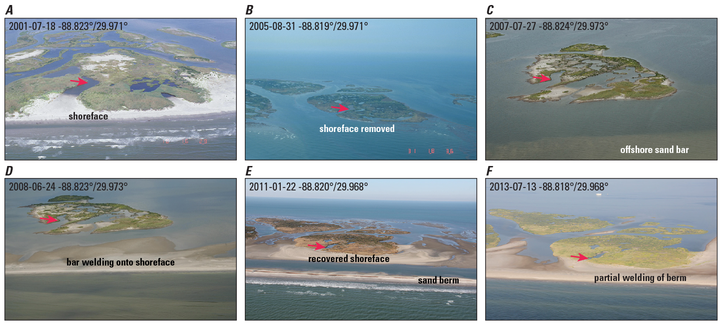
Aerial photographs (A–F) of the Chandeleur Islands, Louisiana, with date-time and latitude-longitude stamping in the upper-left corner of the image (U.S. Geological Survey, variously dated). Hurricane Katrina was a major erosion event for the Chandeleur Islands in 2005. This series of aerial photographs shows (A) the same islets 4 years before (2001) and (B–F) up to 8 years (2005–2013) after impact. For reference, the red arrow points to the same geographic position in each frame. The viewpoint is from the Gulf side of the islands looking west; the coordinates reflect the position of the aircraft, which is often in the same position for each frame but at slightly different altitudes and viewing angles. During Hurricane Katrina, waves and storm surge completely submerged the islands, and (B) removed any available sand, leaving only marsh. Without the sandy shoreface (C) the islands continued to deteriorate for 2 years after the storm. Sand that was moved into the Gulf (C) began to stack into offshore bars, which (D) eventually welded onto the island shoreface. In 2011, the (E) Deepwater Horizon oil spill mitigation sand berm was constructed immediately offshore of the northern Chandeleur Islands. Although most of the berm sediment was immediately transported north toward Hewes Point, (F) portions of the berm welded onto the island shoreface.
Through this recovery process, the subaerial islands gained approximately 44×106 m3 of sediment (table 5 and fig. 21, polygons 35 and 40) between 2007 and 2015, with the sand berm project contributing up to 8 percent of the total. Breton Island recovered slightly, gaining 1×10⁶ m3 of sediment (table 5 and fig. 21, polygon 26), and the Grand Gosier Shoals also reemerged, accreting almost 6×10⁶ m3 of sediment. These shoals experienced the highest gain per unit area across the study area (table 5 and fig. 21, polygons 30 and 31).
Compared to the long-term (1920–2007) period, the recent, short term (2007–2015) period reflects similar large-scale morphologic trends. Significant erosion occurred along the seaward side of the islands, with deposition on the Sound side of the island platform. Sediment accretion through littoral sediment transport is present south of Grand Gosier Shoals during both periods, as well to the north at Hewes Point (fig. 21).
Error Analysis
The DEM for each period was compared with the data points used to generate the DEM to determine the error associated with the gridding process. From this comparison, the root mean square (RMS) error was calculated for each DEM and reported in table 6. The GMT tools “grdtrack,” “gmtinfo,” and “grdinfo” were used to extract the datapoint positions from the DEM grid cells and generate the statistics for each dataset and DEM. The RMS error ranged from 0.03 to 0.24 m, with the highest value coming from the 2006–2007 bathymetric DEM. It should be noted that, due to the coarse grid resolution, the greatest amount of error likely occurs where gradients are high, such as along the shoreface or within the borrow pit. Also, areas where data points are sparse, such as between bathymetric tracklines, introduce a higher uncertainty into the DEM than areas of high data density, such as the lidar point cloud (Amante, 2018).
Small amounts of change—when the difference in elevation between two periods is close to zero—are considered to be within the range of uncertainty and are not considered; this ensures a conservative estimate for volumetric-change calculations. For this study, the range of uncertainty (error) is ±0.25 m and is excluded when calculating the volumetric change between periods for each littoral-cell polygon. The volume within the error range is reported as error in tables 4 and 5. The GMT “grdvolume” tool was used to calculate this volume for each littoral-cell polygon. Cells that experienced relatively small amounts of volumetric change between periods generally produced higher uncertainties.
Table 6.
Cell statistics and root mean square error values calculated for each dataset. Elevation values are referenced to North American Vertical Datum of 1988.[m, meter; DEM, digital elevation model; RMS, root-mean square]
Sediment Budget Calculation
The sediment transport processes responsible for the sediment distribution across the islands are (1) littoral sediment transport driven by both storm and nonstorm wave action and (2) the cross-shore transport of sediment through overwash during extreme storms. Models of sediment transport along the Chandeleur Islands indicate a bidirectional littoral system, with net northward sediment transport along the northern half of the island chain and net southward transport to the south (fig. 23). Transport magnitudes range from 5×10⁴ m3/yr to 1.3×10⁵ m3/yr in both directions (Ellis and Stone, 2006; Georgiou and Schindler, 2009), with tropical storms dominating sediment transport (fig. 23). These magnitudes and directions only apply to the northern Chandeleur Islands. Wave analysis and the modeling of sediment transport along Breton Island show a net northward-transport rate of 0.5×10⁵ m3/yr along the northern half of the island and up to 1.5×10⁵ m3/yr along the southern half (Dalyander and others, 2017).
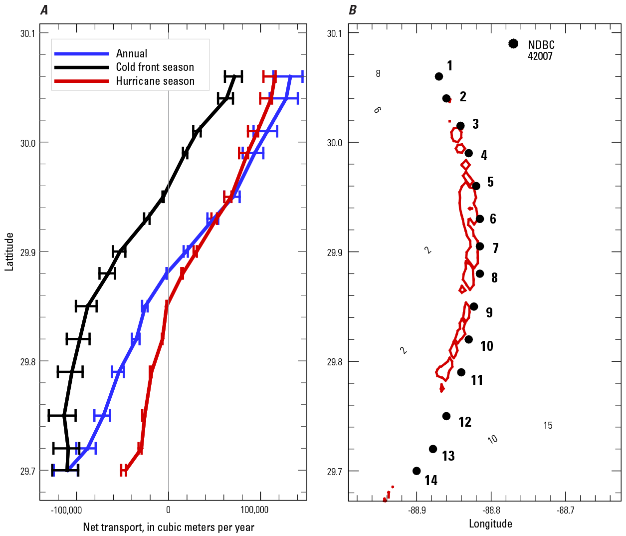
Data plots from Georgiou and Schindler (2009). A. Modeled cumulative longshore-sediment-transport rates and direction (negative values correspond to net southward transport and equal positive values) as a function of annual (net) cold front and hurricane season wave-forcing along the length (vertical scale is latitude) of the Chandeleur Islands, Louisiana (La.). Sediment transport bifurcates from a nodal point at the center of the barrier island arc. B. Locations (latitude and longitude) along the Chandeleur Islands, La., for each model calculation. The National Oceanic and Atmospheric Administration buoy (NDBC 42007) that provided the wave data is also shown. Contours are water depth in meters.
In addition to littoral transport, sediment moves toward the island platform on both the Gulf and Sound sides, driven primarily by storm-associated seafloor scour. These observations create rules by which a sediment-budget alternative can be developed using the cells defined in figures 18 and 21:
-
Littoral sediment transport is to the north at the northern half of the Chandeleur Islands; to the south at the southern half; and southerly at Curlew and Grand Gosier shoals. Breton Island primarily experiences southerly transport but also westerly transport through overwash due to the low elevation of the island.
-
Sediment is lost from the system at Hewes Point and through mechanical dredging of the MRGO (until 2008 when maintenance ceased).
-
Sediment transport by storm-driven wave action is from offshore to onshore (east to west in the Gulf; west to east in the Sound), although significant storms disrupt the system and move sediment offshore.
These processes establish transport pathways necessary to develop a sediment budget, by which sediment is moved between adjacent cells. Tracking sediment flux throughout the system is assisted by use of the “Sediment Budget Analysis System” (SBAS) tool for ArcGIS (U.S. Army Corps of Engineers [USACE], 2018). This tool was developed by the USACE to formulate and calculate sediment flux between sources and sinks. In this model, the net volume change (∆V) per cell is balanced by the flux of sediment into and out of the cell. The SBAS tool tracks the residual value, or balance between the ∆V and the sediment flux (Q), between source (Qsource) and sink (Qsink):
whereQ is the sediment flux,
P is the placement volume (if not applicable = 0), and
R is the removal volume (if not applicable = 0).
The SBAS tool converts each polygon, or cell, to a feature in ArcMap. These features are each assigned a value, ∆V, P, and R, and stored in the littoral-cell layer (fig. 24). Sediment pathways between cells are represented by vector layers (arrows) with a flux direction and assigned a Q value. The vectors are stored in the flux layer and linked to the littoral-cell layer through an attribute table. The SBAS tool updates the attribute table to track the residual equation fields for each cell. The residual value approaches zero as the sediment budget within each field is balanced. In the example shown in figure 24, the difference between ∑Qsource and ∑Qsink balance ∆V with a residual of −5 m3 (0.0001 percent of ∆V).
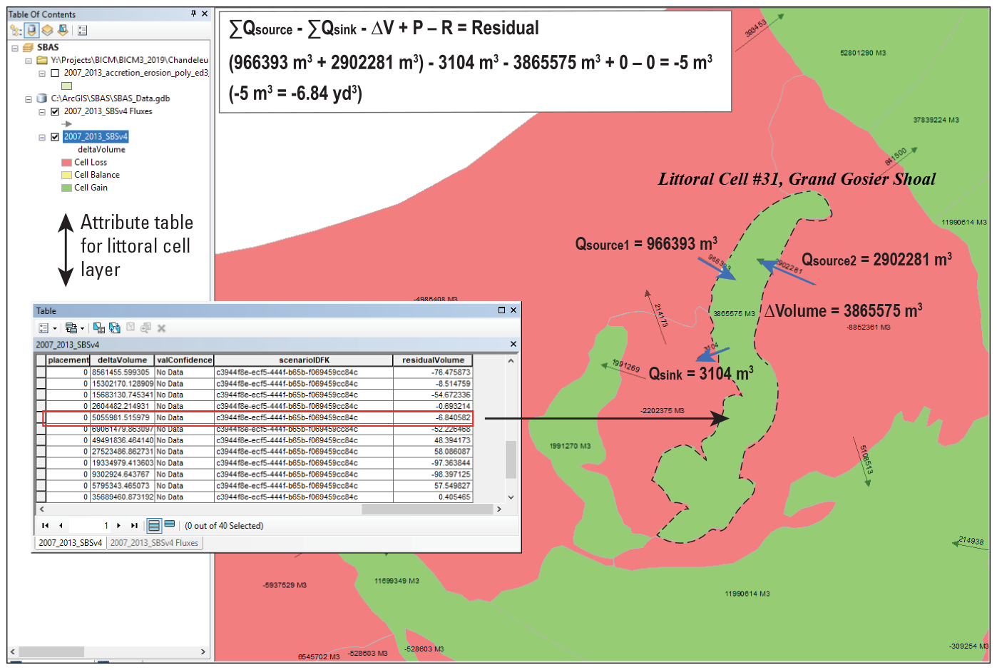
Screenshot showing example of the “Sediment Budget Analysis System” tool in ArcGIS tracking the sediment budget for the 2007–2015 period. The polygons represent the accretion (green) and erosion (red) cells and are attributed with the net volume change (∆V). Polygon 31 (table 5) represents the littoral cell for Grand Gosier Shoals (fig. 21). The residual volume in the cell approaches zero as the sediment flux (Q) into and out of the cell is balanced.
The sediment fluxes between Qsource and Qsink for the two periods are shown in figures 25 and 26, and the associated ∆V, Qsource and Qsink, and residual volume statistics are shown in tables 7 and 8. Arrows on the maps indicate the direction of flux from the cell source (Qsource) to the cell sink (Qsink). Residual values (tables 7 and 8) represent the sediment remaining (positive value) or missing (negative value) after ∆V is balanced by Qsource and Qsink. These values vary by cell but are essentially zero when compared to ∆V, which indicates a balanced sediment budget.
Map of littoral cells for the 1920–2007 period, where the net volume change (∆V) is positive (green) or negative (red). Blue arrows represent flux direction from (Qsource) and to (Qsink) the cell. The resulting residual volume over the period is calculated by the “Sediment Budget Analysis System” (SBAS) tool and reported in table 7. MRGO, Mississippi River to Gulf Outlet.
Table 7.
Net volume change (∆V) per accretion-erosion cell (polygon) calculated from the 1920–2007 period (see figure 25 for location of cells). The sediment flux from (Qsource) and to (Qsink) the cell represents the sediment volumes necessary to balance the sediment budget within the cell, reflected by the residual volume.[∆V, net volume change; Q, sediment flux; m3, cubic meter]
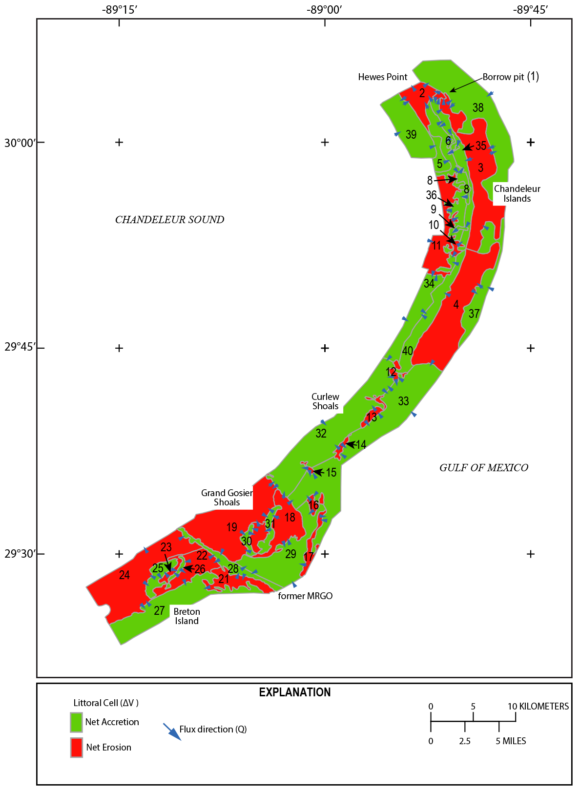
Map of littoral cells for the 2007–2015 period, where the net volume change (∆V) is positive (green) or negative (red). Blue arrows represent sediment flux direction from (Qsource) and to (Qsink) the cell. The resulting residual volume over the period is calculated by the “Sediment Budget Analysis System” (SBAS) tool and reported in table 8.
Table 8.
Net volume change (∆V) per accretion-erosion cell (polygon) calculated from the 2007–2015 period (see figure 26 for location of cells). The sediment flux from (Qsource) and to (Qsink) the cell represents the sediment volumes necessary to balance the sediment budget within the cell, reflected by the residual volume.[∆V, net volume change; Q, sediment flux; m3, cubic meter]
The regional budgets for the study area contrast sharply between the 1920–2007 and 2007–2015 periods. The budget for the later period (2007–2015) cannot be balanced without sediment input from outside the study area, represented by the input-flux arrows in figure 26. As discussed earlier, the sediment input likely reflects the recovery period after Hurricane Katrina, as sand returns to the island platform through lateral bar accretion (fig. 22C, D). The later period also includes the construction of the Deepwater Horizon oil spill mitigation sand berm (Plant and others, 2014).
Sand was excavated from a borrow pit at Hewes Point (fig. 21, polygon 1) and conveyed by pipeline to the island shoreface (table 9). The berm (fig. 22E), known as E4, extended immediately offshore of the island for 8 km then joined the island shoreline for an additional 4 km (fig. 27). Construction volumes submitted to the USACE estimate 4.1×10⁶ m3 of sediment was used to construct the berm; of that amount, 0.5×10⁶ m3 was mined from an alternate borrow pit known as “Borrow Area 6A”; see figure 27 for the location. These data correspond well to the estimate from this study of 3.02×10⁶ m3 removed from the borrow site (table 5, polygon 1). For the sediment budget calculation, this amount was contributed directly to the island platform cell (fig. 26, polygon 40). Sediment is lost from the system through Hewes Point (fig. 26, polygon 2). Approximately 4.1×10⁶ m3 of sediment exits Hewes Point to the north, at a rate of about 0.6×10⁶ m3/yr.
Table 9.
Dredging operations that occurred throughout the study area for channel construction and maintenance, oil spill mitigation, and beneficial use restoration, with estimated sediment volumes.[La., Louisiana; MRGO, Mississippi River to Gulf Outlet; m3, cubic meter]
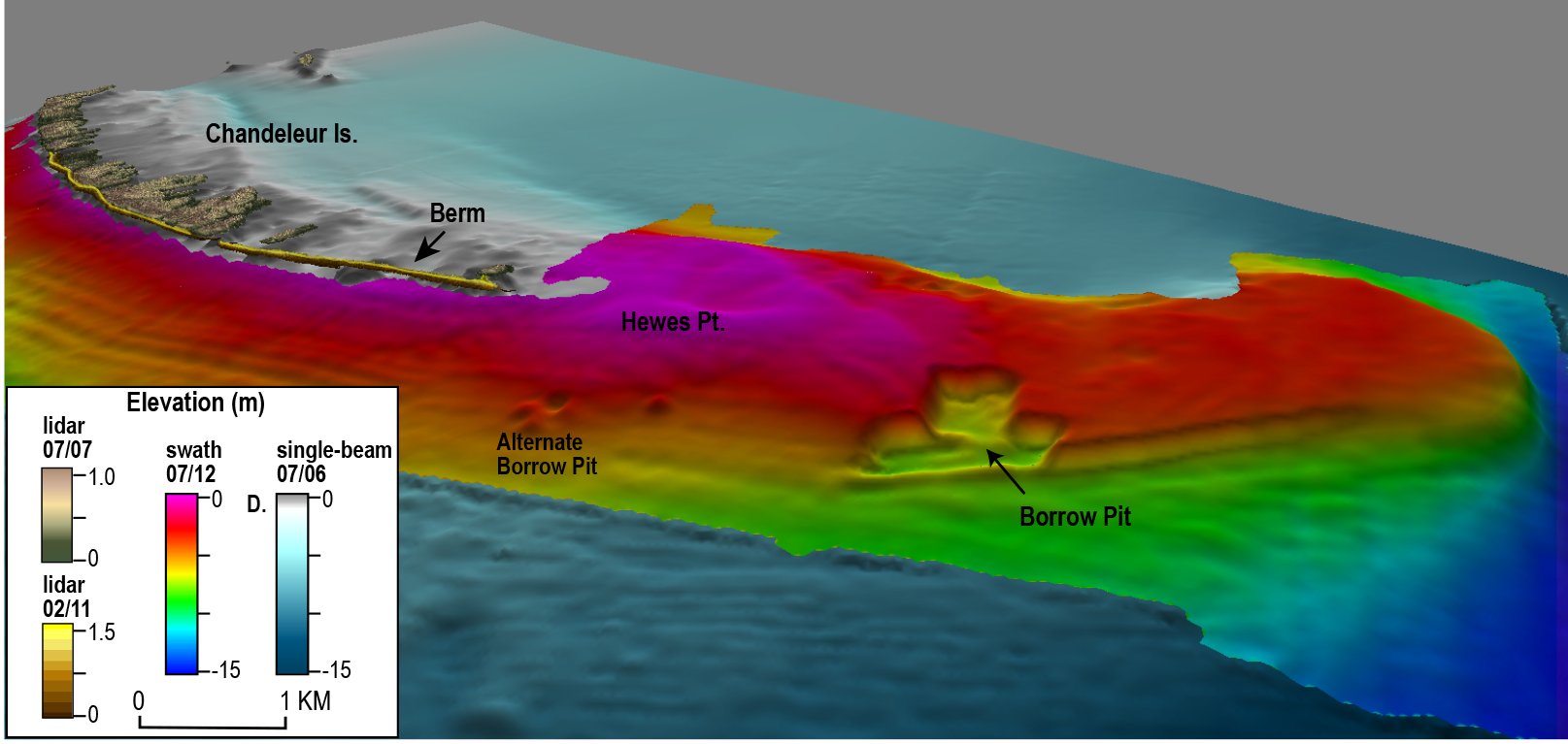
Perspective image of the Chandeleur Islands, Louisiana, Deepwater Horizon oil spill mitigation sand berm and surrounding seafloor. The borrow pit excavated to provide the sand for the berm is visible in the 2012 bathymetry, as is an alternate borrow pit initially excavated for sand and later filled with sediment from the main borrow pit. The image compiles various elevation datasets including light detection and ranging (lidar) topography of the islands (2007) and the berm (2011), interferometric-swath and single-beam bathymetry of the surrounding waters (2006) and of Hewes Point and nearshore (2012). Modified from Plant and others (2014).
The sediment budget for the 1920–2007 period conserves sediment with no input from outside the study area (fig. 25). Approximately 114×106 m3 of sediment exits the system at Hewes Point, or 1.3×10⁶ m3/yr. The long-term sediment flux north of Hewes Point is much higher than that of the recent, short term (2007–2015) flux. This higher flux is likely due to the impact of major hurricanes (such as Camille, Ivan, and Katrina), whereas the more recent period had few storms (Terrano and others, 2016). At the southern end of the study area, the long-term period includes the excavation of the MRGO shipping channel, which began in 1958 and was completed in 1968 (USACE, 2012). In a study of MRGO ecosystem restoration, it is estimated that 90×106 m3 of sediment was removed from the MRGO and placed in an offshore disposal site during periods of construction and maintenance between the 1960s and 2004 (Thomson and others, 2009). This volume is not relevant to this study, as the disposal volume would include sediments removed from channel lengths not within the study area.
For this study, it is calculated that approximately 26×106 m3 of sediment was removed during construction of the ship channel (tables 4 and 9). The channel was periodically re-dredged, and the sediment was placed in an offshore disposal site to maintain a navigable-waterway depth. The MRGO site-disposal data estimate that 72×106 m3 of sediment was removed from the MRGO between 1976 and 2005; but, as mentioned above, this includes areas outside the study area. Not all of the sediment was disposed of offshore. As part of a beneficial use project, sediment was removed from the channel and placed adjacent to Breton Island in 1993, 1999, and 2001 (Creef and others, 2003). The three placements amount to 6.5×10⁶ m3 of sediment and are accounted for in the budget analysis as a single direct-sediment flux from the MRGO to Breton Island (bypassing littoral-cell polygons 17 and 19 [fig. 25]). The sediment-budget analysis estimates that a total of 37×106 m3 of sediment was removed from the MRGO within the study area (table 9). The balance of the estimated sediment flux, renourishment volumes to Breton Island, and excavation volume suggests that within the study area 16.5×10⁶ m3 of sediment was removed from the MRGO to maintain the authorized navigable-waterway depth between 1968 and 2007.
Final Sediment-Budget Summary
A comparison of sediment flux over the two periods shows the three following conclusions.
-
Sediment removal from the system—In the northernmost Chandeleur Islands, the largest sediment loss from the barrier island system is through littoral transport north to Hewes Point. Over the study period (1920–2013) approximately 115×106 m3 of sediment was transported north. Geophysical assessment of the sand spit at Hewes Point (Flocks and others, 2009b) estimates a volume of approximately 340×106 m3. This suggests that over 30 percent of the sand spit was deposited over the past 100 years (meaning that northward sediment transport rates increased since historical time). The islands have reached a collapsed stage (Penland and others, 1988) where sand previously sequestered in beach and dune deposits is increasingly released into the littoral system. The sediment deposited at Hewes Point is generally over 90 percent sand (Flocks and others, 2009a) and can be recovered for restoration of the island’s elevation.
-
Throughout the rest of the study area (the central Chandeleur Islands to Breton Island), over the long-term study period (1920–2007), sediment is conserved within the system, and rollover processes are the dominant transport mechanism (see list item 3 below). Other sediment processes include mechanical dredging at Hewes Point to construct a temporary sand berm along the northern Chandeleur Islands—which has remained in the system or returned to Hewes Point—and the construction and maintenance of the MRGO (see list item 4 below).
-
Overwash—Most of the morphologic change along the Chandeleur Islands occurs through rollover processes such as overwash. Over the 1920–2007 period, this overwash is represented by the sediment flux from polygon 9 to polygon 4 (fig. 25), where approximately 109×106 m3 of sediment, or 1.25×10⁶ m3/yr, transported westward. Over the 2007–2013 period—represented by sediment flux from polygon 3 to 35 and from 4 to 40 (fig. 26)—approximately 42×106 m3 of sediment transported westward and at a much higher rate (7.2×10⁶ m3/yr) than in the earlier period. This result is likely because, after Hurricane Katrina, there is much less vegetation (for example, mangroves) and elevation (for example, dunes) on the islands to impede overwash processes, and breaches are more prevalent (Martinez and others, 2009). Revegetation and restoration of island elevation is necessary for mitigating rollover. The introduction of sand into the littoral system at the nodal point (fig. 23) along the Chandeleur barrier island arc would use the natural hydrodynamic system to close inlets and enhance shoreface resilience. Direct placement of sand at the foredune uses aeolian and run-up processes to restore island elevation.
-
To the south, Curlew Shoals, Grand Gosier Shoals, and Breton Island are also experiencing rollover processes. At Breton Island, over the study period (1920–2013), approximately 11×106 m3 of sediment transported westward—from polygon 19 to 15 (fig. 25), and from polygon 20 to 24 (fig. 26)—at a much slower rate (116,000 m3/yr) compared with the Chandeleur Islands. A sand deposit was identified offshore of Breton Island that supports the mitigation of rollover processes (Dalyander and others, 2017). This deposit contains up to 3 m of 85–95 percent sand (Bernier and others, 2017) and possibly represents a long-submerged southern extent of the Chandeleur Island barrier chain.
-
Dredging of MRGO—Excavation of the MRGO ship channel was completed in 1968. Within the study area, approximately 26×106 m3 of sediment was removed and disposed of offshore. This offshore deposit was not identified during an extensive geophysical investigation of the waters surrounding Breton Island (DeWitt and others, 2016). Sediment cores collected from in and around the MRGO are composed primarily of laminated muds (Bernier and others, 2017), which, in disposal sites, would have likely been reworked by currents. The MRGO was decommissioned in 2006 and has since infilled with sediment (fig. 20), suggesting no mitigation is necessary. Tidal dynamics between Grand Gosier Shoals and Breton Island have likely changed due to the infilling of the channel. Littoral transport across the former channel is evident at Grand Gosier Shoals; since 2007, approximately 3.8×10⁶ m3 of sediment migrated from the shoal area (polygon 19, fig. 26) to the former channel location (polygon 28, fig. 26). This littoral transport of sediment away from Grand Gosier Shoals occurred throughout the life of the MRGO, as evidenced by the large amount of sediment accretion adjacent to the channel since the 1920s (fig. 18). This sediment is no longer mechanically removed by channel maintenance (16.5×10⁶ m3 within the study area) and is expected to remain within the system.
References Cited
Amante, C., 2018, Estimating coastal digital elevation model uncertainty: Journal of Coastal Research, v. 34, p. 1382–1397, accessed October 29, 2020, at https://doi.org/10.2112/JCOASTRES-D-17-00211.1.
Baldwin, W.E., Pendleton, E.A., and Twichell, D.C., 2009, Geophysical data from offshore of the Chandeleur Islands, Eastern Mississippi Delta: U.S. Geological Survey Open-File Report 2008–1195, accessed October 29, 2020, at https://doi.org/10.3133/ofr20081195.
Bernier, J.C., Kelso, K.W., Tuten, T.M., Stalk, C.A., and Flocks, J.G., 2017, Sediment data collected in 2014 and 2015 from around Breton and Gosier Islands, Breton National Wildlife Refuge, Louisiana: U.S. Geological Survey Data Series 1037, accessed September 2, 2018, at https://doi.org/10.3133/ds1037.
Buster, N.A., and Morton, R.A., 2011, Historical bathymetry and bathymetric change in the Mississippi-Alabama coastal region, 1847–2009: U.S. Geological Survey Scientific Investigations Map 3154, 1 sheet, 13-p. pamphlet, accessed October 29, 2020, at https://doi.org/10.3133/sim3154.
Byrnes, M.R., Berlinghoff, J.L., Griffee, S.F., and Lee, D.M., 2018, Final Report—Louisiana Barrier Island Comprehensive Monitoring Program (BICM)—Phase 2—Updated shoreline compilation and change assessment, 1880s to 2015: Louisiana Coastal Protection and Restoration Authority (CPRA) report, prepared by Applied Coastal Research and Engineering, Mashpee, Mass., and Metairie, La., in cooperation with CDM Smith, [Boston, Mass.,] 46 p., accessed October 29, 2020, at https://www.lacoast.gov/reports/project/20180812_BICM_Phase2_Final_Report_plus_Appendices.pdf.
Coastal Protection and Restoration Authority of Louisiana, 2016, Coastal Information Management System (CIMS)—File naming convention (ver. 1.8): Coastal Protection and Restoration Authority report, 9 p., accessed November 11, 2016, at http://mrhdms.coastal.louisiana.gov/site/docs/CPRACIMSFileNamingConvention_v1_8.pdf.
Creef, E.D., Mathies, L.G., and Hennington, S.M., 2003, Breton Island restoration project, in Garbaciak, S., Jr., ed., Dredging '02—Key technologies for global prosperity, Third Specialty Conference on Dredging and Dredged Material Disposal, May 5–8, 2002, Orlando, Florida, proceedings: Reston, Va., American Society of Civil Engineers, 5 p., accessed October 11, 2018, at https://doi.org/10.1061/40680(2003)13.
Dalyander, P.S., Mickey, R.C., Long, J.W., and Flocks, J.G., 2017, Effects of proposed sediment borrow pits on nearshore wave climate and longshore sediment transport rate along Breton Island, Louisiana (ver. 2.0, August 2017): U.S. Geological Survey Open-File Report 2015–1055, 41 p., accessed September 20, 2018, at https://doi.org/10.3133/ofr20151055.
DeWitt, N.T., Miselis, J.L., Fredericks, J.J., Bernier, J.C., Reynolds, B.J., Kelso, K.W., Thompson, D.M., Flocks, J.G., and Wiese, D.S., 2017, Coastal bathymetry data collected in 2013 from the Chandeleur Islands, Louisiana: U.S. Geological Survey Data Series 1032, accessed September 20, 2018, at https://doi.org/10.3133/ds1032.
DeWitt, N.T., Fredericks, J.J., Flocks, J.G., Miselis, J.L., Locker, S.D., Kindinger, J.G., Bernier, J.C., Kelso, K.W., Reynolds, B.J., Wiese, D.S., and Browning, T., 2016, Archive of bathymetry and backscatter data collected in 2014 nearshore Breton and Gosier Islands, Breton National Wildlife Refuge, Louisiana: U.S. Geological Survey Data Series 1005, accessed September 20, 2018, at https://doi.org/10.3133/ds1005.
Digital Aerial Solutions, [2016], LiDAR project report, G15PD00057, South Terrebonne and Gulf Islands, QL2 lidar: U.S. Geological Survey report, prepared by Digital Aerial Solutions, LLC, Tampa, Fla., under contract no. G10PC00093, [variously paged; 68 p.], accessed October 11, 2018, at https://www.maris.state.ms.us/HTML/DATA/data_Elevation/REPORTS/G15PD00057,%20South%20Terrebonne%20and%20Gulf%20Islands%20QL2%20LiDARProject_Report.pdf.
Ellis, J., and Stone, G.W., 2006, Numerical simulation of net longshore sediment transport and granulometry of surficial sediments along Chandeleur Island, Louisiana, USA: Marine Geology, v. 232, nos. 3–4, p. 115–129, accessed October 29, 2020, at https://doi.org/10.1016/j.margeo.2006.05.001.
Fagherazzi, S., Carniello, L., D’Alpaos, L., and Defina, A., 2006, Critical bifurcation of shallow microtidal landforms in tidal flats and salt marshes: Proceedings of the National Academy of Sciences of the United States of America, v. 103, no. 22, p. 8337–8341, accessed October 29, 2020, at https://doi.org/10.1073/pnas.0508379103.
Fearnley, S.M., Miner, M.D., Kulp, M., Bohling, C., and Penland, S., 2009, Hurricane impact and recovery shoreline change analysis of the Chandeleur Islands, Louisiana, USA—1855 to 2005: Geo-Marine Letters, v. 29, no. 6, p. 455–466, accessed October 29, 2020, at https://doi.org/10.1007/s00367-009-0155-5.
FitzGerald, D.M., Georgiou, I., and Kulp, M., 2016, Restoration of the Chandeleur Barrier Arc, Louisiana: Journal of Coastal Research, v. 75, Special issue no. 1, p. 1282–1286, accessed October 29, 2020, at https://doi.org/10.2112/SI75-257.1.
Flocks, J.G., and Terrano, J.F., 2016, Analysis of seafloor change at Breton Island, Gosier Shoals, and surrounding waters, 1869–2014, Breton National Wildlife Refuge, Louisiana: U.S. Geological Survey Open-File Report 2016–1069, 27 p., accessed September 18, 2018, at https://doi.org/10.3133/ofr20161069.
Flocks, J., Twichell, D., Sanford, J., Pendleton, E., and Baldwin, W., 2009a, Sediment sampling analysis to define quality of sand resources, chap. F. in Lavoie, D., ed., Sand resources, regional geology, and coastal processes of the Chandeleur Islands coastal system—An evaluation of the Breton National Wildlife Refuge: U.S. Geological Survey Scientific Investigations Report 2009–5252, p. 99–124, accessed September 18. 2018, at https://pubs.usgs.gov/sir/2009/5252/downloads/Chapter-F/Chapter-F.pdf.
Flocks, J., Twichell, D., Pendleton, E., Baldwin, W., and Miner, M., 2009b, The geologic framework of the Chandeleur Islands, Louisiana—Insight into the history and fate of a fragile ecosystem [abs.]: Geological Society of America Abstracts with Programs, v. 41, no. 1, p. 8. [Also available at https://gsa.confex.com/gsa/2009SE/webprogram/Paper154863.html.]
Forde, A.S., Flocks, J.G., Wiese, D.S., and Fredericks, J.J., 2016, Archive of digital chirp subbottom profile data collected during USGS cruise 14BIM05 offshore of Breton Island, Louisiana, August 2014: U.S. Geological Survey Data Series 972, accessed September 18, 2018, at https://doi.org/10.3133/ds972. [Also available on 2 DVDs.]
Frazier, D., 1967, Recent deltaic deposits of the Mississippi River—Their development and chronology: Gulf Coast Association of Geological Societies Transactions, v. 17, p. 287–315. [Also available at https://archives.datapages.com/data/gcags/data/017/017001/0287.htm.]
Georgiou, I.Y., and Schindler, J., 2009, Numerical simulation of waves and sediment transport along a transgressive barrier island, chap. H in Lavoie, D., ed., Sand resources, regional geology, and coastal processes of the Chandeleur Islands coastal system—An evaluation of the Breton National Wildlife Refuge: U.S. Geological Survey Scientific Investigations Report 2009–5252, p. 143–168, accessed July 6, 2017, at https://pubs.usgs.gov/sir/2009/5252/downloads/Chapter-H/Chapter-H.pdf.
Kindinger, J.L., Buster, N.A., Flocks, J.G., Bernier, J.C., and Kulp, M.A., 2013, Louisiana Barrier Island Comprehensive Monitoring (BICM) program summary report—Data and analyses 2006 through 2010: U.S. Geological Survey Open-File Report 2013–1083, 86 p, accessed October 18, 2018, at https://doi.org/10.3133/ofr20131083.
Lavoie, D., Flocks, J.G., Kindinger, J.L., Sallenger, A.H., Jr., and Twichell, D.C., 2010, Effects of building a sand barrier berm to mitigate the effects of the Deepwater Horizon oil spill on Louisiana marshes: U.S. Geological Survey Open-File Report 2010–1108, 7 p., accessed October 18, 2018, at https://doi.org/10.3133/ofr20101108.
Lavoie, D., ed., 2009, Sand resources, regional geology, and coastal processes of the Chandeleur Islands coastal system—An evaluation of the Breton National Wildlife Refuge: U.S. Geological Survey Scientific Investigations Report 2009–5252, 180 p., accessed July 6, 2017, at https://doi.org/10.3133/sir20095252.
Martinez, L., O’Brien, S., Bethel, M., Penland, S., and Kulp, M., 2009, Louisiana Barrier Island Comprehensive Monitoring Program (BICM) volume 2—Shoreline changes and barrier island land loss 1800’s–2005: New Orleans, La., Pontchartrain Institute for Environmental Sciences, University of New Orleans, Pontchartrain Institute Reports and Studies paper no. 1, 32 p., accessed November 17, 2020, at https://scholarworks.uno.edu/cgi/viewcontent.cgi?referer=https://scholar.google.com/&httpsredir=1&article=1000&context=pies_rpts.
Miner, M., Kulp, M., Penland, S., Weathers, D., Motti, J.P., McCarty, P., Brown, M., Martinez, L., Torres, J., Flocks, J.G., DeWitt, N., Ferina, N., Reynolds, BJ., Twichell, D., Baldwin, W., Danforth, B., Worley, C., and Bergeron, E., 2009a, Louisiana Barrier Island Comprehensive Monitoring Program (BICM) Volume 3—Bathymetry and historical seafloor change 1869–2007, part 1—South‐central Louisiana and northern Chandeleur Islands, bathymetry methods and uncertainty analysis—Final report: New Orleans, La., Pontchartrain Institute for Environmental Sciences, University of New Orleans, Funded through Louisiana Department of Natural Resources [LDNR] and U.S. Army Corps of Engineers (as LCA Science & Technology Program) through LDNR interagency agreement 2512–06–06, 45 p., accessed November 17, 2020, at https://scholarworks.uno.edu/cgi/viewcontent.cgi?article=1006&context=pies_rpts.
Miner, M., Kulp, M., Weathers, D., Mottie, J., McCarty, P., Brown, M., Torres, J., Martinez, L., Flocks, J., DeWitt, N., Reynolds, B., Twichell, D., Baldwin, W., Danforth, B., Worley, C., and Bergeron, E., 2009b, Louisiana Barrier Island Comprehensive Monitoring Program (BICM) Volume 3—Bathymetry and historical seafloor change, 1869–2007, part 3—Southern Chandeleur Islands and western Chenier beaches, bathymetry maps—Final report: New Orleans, La., Pontchartrain Institute for Environmental Sciences, University of New Orleans, Funded through Louisiana Department of Natural Resources [LDNR] and U.S. Army Corps of Engineers (as LCA Science & Technology Program) through LDNR interagency agreement 2512–06–06, 16 p., accessed October 29, 2020, at https://www.lacoast.gov/reports/project/BICM3_part3_SouthernChandeleurIs_WestChenBeachesBathy.pdf.
Miselis, J.L., Long, J.W., Dalyander, P.S., Flocks, J.G., Buster, N.A., and Mickey, R.C., 2015, Integrating geophysical and oceanographic data to assess interannual variability in longshore sediment transport, in Wang, P., Rosati, J.D., and Cheng, J., eds., Proceedings of the Coastal Sediments 2015, San Diego, USA, May 11–15, 2015: Hackensack, N.J., World Scientific, p. 113–126, accessed October 28, 2021, at https://doi.org/10.1142/9789814689977_0011.
National Centers for Environmental Information [NCEI], 1918, Report for H04000: National Oceanic and Atmospheric Administration website, accessed October 11, 2018, at https://www.ngdc.noaa.gov/nos/H02001-H04000/H04000.html.
National Centers for Environmental Information [NCEI], 1921, Report for H04171: National Oceanic and Atmospheric Administration website, accessed October 11, 2018, at https://www.ngdc.noaa.gov/nos/H04001-H06000/H04171.html.
National Centers for Environmental Information [NCEI], 1922a, Report for H04212: National Oceanic and Atmospheric Administration website, accessed October 11, 2018, at https://www.ngdc.noaa.gov/nos/H04001-H06000/H04212.html.
National Centers for Environmental Information [NCEI], 1922b, Report for H04219: National Oceanic and Atmospheric Administration website, accessed October 11, 2018, at https://www.ngdc.noaa.gov/nos/H04001-H06000/H04219.html.
National Centers for Environmental Information [NCEI], 1922c, Report for H04223: National Oceanic and Atmospheric Administration website, accessed October 11, 2018, at https://www.ngdc.noaa.gov/nos/H04001-H06000/H04223.html.
National Centers for Environmental Information [NCEI], 1940, Report for H06552: National Oceanic and Atmospheric Administration website, accessed October 11, 2018, at https://www.ngdc.noaa.gov/nos/H06001-H08000/H06552.html.
National Centers for Environmental Information [NCEI], 2014, Report for H12528: National Oceanic and Atmospheric Administration website, accessed October 28, 2021, at https://www.ngdc.noaa.gov/nos/H12001-H14000/H12528.html.
National Centers for Environmental Information [NCEI], 2015, Report for H12711: National Oceanic and Atmospheric Administration website, accessed October 28, 2021, at https://www.ngdc.noaa.gov/nos/H12001-H14000/H12711.html.
National Centers for Environmental Information [NCEI], 2016, Report for H12847: National Oceanic and Atmospheric Administration website, accessed October 28, 2021, at https://www.ngdc.noaa.gov/nos/H12001-H14000/H12847.html.
National Oceanic and Atmospheric Administration [NOAA], 2017, Relative sea level trends for tropical and Gulf of Mexico web page: NOAA Tides & Currents website, accessed December 2, 2018, at https://tidesandcurrents.noaa.gov/sltrends/regionalcomparison.html?region=USTG.
National Oceanic and Atmospheric Administration [NOAA], 2020, Relative sea level trend—8729840 Pensacola, Florida, web page: NOAA Tides & Currents website, accessed January 04, 2022, at https://tidesandcurrents.noaa.gov/sltrends/sltrends_station.shtml?id=8729840.
Otvos, E.G., 1981, Barrier island formation through nearshore aggradation—Stratigraphic and field evidence: Marine Geology, v. 43, nos. 3–4, p. 195–243, accessed October 20, 2020, at https://doi.org/10.1016/0025-3227(81)90181-X.
Penland, S., Boyd, R., and Suter, J.R., 1988, Transgressive depositional systems of the Mississippi Delta plain—A model for barrier shoreline and shelf sand development: Journal of Sedimentary Petrology, v. 58, no. 6, p. 932–949, accessed October 29, 2020, at https://doi.org/10.1306/212F8EC2-2B24-11D7-8648000102C1865D.
Plant, N.G., Flocks J.G., Stockdon, H.F., Long, J.W., Guy, K., Thompson, D.M., Cormier, J.M., Smith, C.G., Miselis, J.L., and Dalyander, P.S., 2014, Predictions of barrier island berm evolution in a time-varying storm climatology: Journal of Geophysical Research, Earth Surface, v. 119, no. 2, p. 300–316, accessed October 29, 2020, at https://doi.org/10.1002/2013JF002871.
Poirrer, M.A., 2007, Statewide Summary for Louisiana, in Handley, L., Altsman, D., and DeMay, R. eds., Seagrass status and trends in the northern Gulf of Mexico—1940–2002 (ver. 1.0, June 2007): U.S. Geological Survey Scientific Investigations Report 2006–5287, p. 61–62, accessed October 29, 2020, at https://doi.org/10.3133/sir20065287. [Report also available as U.S. Environmental Protection Agency 855–R–04–003.]
Poirrer, M.A., and Handley, L.R., 2007, Chandeleur Islands, in Handley, L., Altsman, D., and DeMay, R. eds., Seagrass status and trends in the northern Gulf of Mexico—1940–2002 (ver. 1.0, June 2007): U.S. Geological Survey Scientific Investigations Report 2006–5287, p. 63–72, accessed October 29, 2020, at https://doi.org/10.3133/sir20065287. [Report also available as U.S. Environmental Protection Agency 855–R–04–003.]
Reyes, E., Georgiou, I., Reed, D., and McCorquodale, A., 2005, Using models to evaluate the effects of barrier islands on estuarine hydrodynamics and habitats—A numerical experiment: Journal of Coastal Research, Special issue no. 44, p. 176–185, accessed October 29, 2020, at https://www.jstor.org/stable/25737056.
Rogers, B.E., Kulp, M.A., and Miner, M.D., 2009, Late Holocene chronology, origin, and evolution of the St. Bernard Shoals, Northern Gulf of Mexico, USA: Geo-Marine Letters, v. 29, no. 6, p. 379–394, accessed October 29, 2020, at https://doi.org/10.1007/s00367-009-0162-6.
Sallenger, A.H., Jr., Wright, C.W., Howd, P., Doran, K., and Guy, K., 2009, Extreme coastal changes on the Chandeleur Islands, Louisiana, during and after Hurricane Katrina, chap. B of Lavoie, D., ed., Sand resources, regional geology, and coastal processes of the Chandeleur Islands coastal system—An evaluation of the Breton National Wildlife Refuge: U.S. Geological Survey Scientific Investigations Report 2009–5252, p. 27–36, accessed July 6, 2017, at https://pubs.usgs.gov/sir/2009/5252/downloads/Chapter-B/Chapter-B.pdf.
Schwab, W.C., Baldwin, W.E., Warner, J.C., List, J.H., Denny, J.F., Liste, M., and Safak, I., 2017, Change in morphology and modern sediment thickness on the inner continental shelf offshore of Fire Island, New York between 2011 and 2014—Analysis of hurricane impact: Marine Geology, v. 391, p. 48–64, accessed October 29, 2020, at https://doi.org/10.1016/j.margeo.2017.07.010.
Smith, K.E., Nayegandhi, A., Wright, C.W., Bonisteel, J.M., and Brock, J.C., 2009, EAARL Coastal Topography—Northern Gulf of Mexico, 2007—Bare Earth: U.S. Geological Survey Data Series 2009–400, accessed 10/28/21, at https://doi.org/10.3133/ds400.
Smith, W., and Wessel, P., 1990, Gridding with continuous curvature splines in tension: Geophysics, v. 55, no. 3, p. 293–305, accessed October 29, 2020, at https://doi.org/10.1190/1.1442837.
Stalk, C.A., DeWitt, N.T., Bernier, J.C., Kindinger, J.G., Flocks, J.G., Miselis, J.L., Locker, S.D., Kelso, K.W., and Tuten, T.M., 2017, Coastal single-beam bathymetry data collected in 2015 from the Chandeleur Islands, Louisiana: U.S. Geological Survey Data Series 1039, accessed October 9, 2018, at https://doi.org/10.3133/ds1039.
Swift, D.J.P., Niederoda, A.W., Vincent, C.E., Hopkins, T.S., 1985, Barrier island evolution, middle Atlantic shelf, U.S.A., part I—Shoreface dynamics: Marine Geology, v. 63, nos. 1–4, p. 331–361, accessed October 29, 2020, at https://doi.org/10.1016/0025-3227(85)90089-1.
Terrano, J.F., Flocks, J.G., and Smith, K.E.L., 2016, Analysis of shoreline and geomorphic change for Breton Island, Louisiana, from 1869 to 2014: U.S. Geological Survey Open-File Report 2016–1039, 34 p., accessed October 18, 2018, at https://doi.org/10.3133/ofr20161039.
Thomson, G., Miner, M., Wycklendt, A., Rees, M., and Swigler, D., 2009, MRGO ecosystem restoration feasibility study—Chandeleur and Breton Islands (revised April 2010): U.S. Army Corps of Engineers report, prepared by Coastal Planning & Engineering, Inc., Boca Raton, Fla., and Pontchartrain Institute for Environmental Sciences, University of New Orleans, New Orleans, La., under contract to URS Group, 96 p.
U.S. Army Corps of Engineers, 2012, Mississippi River Gulf Outlet (MRGO) Ecosystem Restoration Plan—Final feasibility report—Supplemental report of the Chief of Engineers in response to the Water Resources Development Act of 2007: U.S. Army Corps of Engineers report, [variously paged; 285 p.], accessed December 1, 2019, at https://www.mvn.usace.army.mil/Portals/56/docs/environmental/MRGO/MRGOEcosystemRestorationFinalFeasibilityReportJune2012.pdf.
U.S. Army Corps of Engineers, 2018, Sediment Budget Analysis System (SBAS): U.S. Army Corps of Engineers Fact Sheet A–26, 1 p., accessed December 1, 2019, at https://geospatial-usace.opendata.arcgis.com/datasets/d58e0150c30f43b999e77ff89b3bba11.
U.S. Coast and Geodetic Survey [USCGS], 1899, United States Gulf Coast—Chandeleur and Breton Island Sounds, Louisiana (reissued March 1915): U.S. Coast and Geodetic Survey chart 192, 1 sheet, scale 1:80,000, accessed January 04, 2022, at https://www.historicalcharts.noaa.gov/image.php?filename=3N192-15.
U.S. Coast and Geodetic Survey [USCGS], 1922a, [Louisiana, off Mississippi Delta, Chandeleur Islands]: U.S. Coast and Geodetic Survey chart 3917, 1 sheet, scale 1:20,000, accessed January 04, 2022, at https://nosimagery.noaa.gov/images/shoreline_surveys/survey_scans/T-3917.jpg.
U.S. Coast and Geodetic Survey [USCGS], 1922b, [Louisiana, off Mississippi Delta, Chandeleur Islands]: U.S. Coast and Geodetic Survey chart 3918, 1 sheet, scale 1:20,000, accessed January 04, 2022, at https://nosimagery.noaa.gov/images/shoreline_surveys/survey_scans/T-3918.jpg.
U.S. Coast and Geodetic Survey [USCGS], 1922c, [Louisiana, off Mississippi Delta, Errol and Chandeleur Islands]: U.S. Coast and Geodetic Survey chart 3919, 1 sheet, scale 1:20,000, accessed January 04, 2022, at https://nosimagery.noaa.gov/images/shoreline_surveys/survey_scans/T-3919.jpg.
U.S. Coast and Geodetic Survey [USCGS], 1922d, [Louisiana, off Mississippi Delta, Breton Island]: U.S. Coast and Geodetic Survey chart 3920, 1 sheet, scale 1:20,000, accessed January 04, 2022, at https://nosimagery.noaa.gov/images/shoreline_surveys/survey_scans/T-3920.jpg.
U.S. Fish and Wildlife Service [USFWS], 2008, Comprehensive conservation plan—Delta and Breton National Wildlife Refuges—St. Bernard and Plaquemines Parishes, Louisiana: U.S. Fish and Wildlife Service (Southeast Region) report, 140 p., accessed October 18, 2018, at https://www.fws.gov/uploadedFiles/DeltaBretonFinalCCPdoc.pdf.
U.S. Geological Survey, [variously dated], Oblique Aerial Photography Viewer web page: U.S. Geological Survey website, accessed January 04, 2022, at https://www.usgs.gov/media/images/oblique-aerial-photography-viewer.
Wright, L.D., Boon, J.D., Kim, S.C., List, J.H., 1991, Modes of cross-shore sediment transport on the shoreface of the middle Atlantic bight: Marine Geology v. 96, nos. 1–2, p. 19–51, accessed October 29, 2020, at https://doi.org/10.1016/0025-3227(91)90200-N.
Appendix 1. Barrier Island Comprehensive Monitoring Program Products
Topographic and Bathymetric Data Products
The data formats for the Barrier Island Comprehensive Monitoring (BICM) program products are in the numbered list that follows; for specific datasets, see Martinez and others (2009); DeWitt and others (2016); Digital Aerial Solutions (2016); DeWitt and others (2017); and Stalk and others (2017).
-
POINTDATA (or pts): Source data as a three-column American Standard Code for Information Interchange (ASCII) file (UTM_x in meters, UTM_y in meters, elevation in meters). Projected as North American Datum of 1983 (NAD 83) reference frame, with orthometric heights and referenced to North American Vertical Datum of 1988 (NAVD 88) datum using the National Geodetic Survey (NGS) geoid model of 2012 (GEOID12B). Due to the number of points, the 2015 light detection and ranging (lidar) topographic dataset was divided into two ASCII files (north and south). Point distributions of the datasets are shown in figures 3 and 5–8.
-
TIN: Triangulated irregular network (TIN) dataset. The ArcGIS software has a limit of 20 million nodes within the TIN file. The 2015 lidar topographic point clouds exceeded this amount and had to be divided into two TIN files (north and south).
-
RASTER: Raster dataset. These include the Tagged Image File Format (TIFF) image and the associated TIFF world file (TFW). Where necessary, the raster images combined the separate TIN files (above) into one image for each dataset. The raster digital elevation models (DEMs) are shown in figures 9–11.
-
CONTOUR: Contour dataset as a vector shapefile package. Contour attributes are populated according to the Louisiana Coastal Protection and Restoration Authority (CPRA) Coastal Information Management System (CIMS) attribute-labeling convention.
-
METADATA (for each point file, TIN, raster, and contour): Associated metadata files are in the Federal Geographic Data Committee (FGDC) compliant format. Available in ASCII and extensible markup language (XML) formats.
Elevation Change and Sediment Budget Analysis Products
The BICM products for the elevation change analysis and sediment budget analysis are—
-
RASTER: Elevation-change raster map available as TIFF image and associated TFW for the 1920–2007 (bathymetric) and 2007–2015 (topobathymetric) periods.
-
POLYGON: Accretion-erosion cells and associated net volume change (∆V) and residual values for the 1920–2007 and 2007–2015 periods. The polygon files are Esri shapefiles with statistics for each cell stored in the shapefile attribute table. See U.S. Army Corps of Engineers ([USACE], 2018) for a description of the attribute values.
-
VECTOR: Sediment flux direction and magnitude for each cell for the 1920–2007 and 2007–2015 periods. The vector files are Esri shapefiles with each sediment source and sink value (Qvalue) stored within the shapefile attribute table and linked to the polygon attribute table. See USACE (2018) for a description of the attribute values.
Conversion Factors
International System of Units to U.S. customary units
Datum
Vertical coordinate information is referenced to the North American Vertical Datum of 1988 (NAVD 88).
Horizontal coordinate information is referenced to the North American Datum of 1983 (NAD 83).
Altitude, as used in this report, refers to distance above the vertical datum.
Abbreviations
ASCII
American Standard Code for Information Interchange
BICM
Barrier Island Comprehensive Monitoring
BNWR
Breton National Wildlife Refuge
CIMS
Coastal Information Management System
CPRA
Louisiana Coastal Protection and Restoration Authority
DEM
digital elevation model
DOQQ
digital orthophoto quarter quadrangle
FGDC
Federal Geographic Data Committee
GEOID03
geoid model 03
GEOID12A
geoid model 12A
GEOID12B
geoid model 12B
GMT
Generic Mapping Tools
GPS
Global Positioning System
ITRF00
International Terrestrial Reference Frame of 2000
km
kilometer
La.
Louisiana
LAS
LASer [file format]
lidar
light detection and ranging
m
meter
mm
millimeter
MLW
mean low water
MRGO
Mississippi River to Gulf Outlet
NAD 27
North American Datum of 1927
NAD 83
North American Datum of 1983
NAVD 88
North American Vertical Datum of 1988
NCEI
National Centers for Environmental Information
NGS
National Geodetic Survey
NOAA
National Oceanic and Atmospheric Administration
Q
sediment flux
RMS
root mean square
RSLR
relative sea-level rise
s
second
SBAS
Sediment Budget Analysis System
TFW
TIFF world file
TIFF
Tagged Image File Format
TIN
triangulated irregular network
USCGS
U.S. Coast and Geodetic Survey
USFWS
U.S. Fish and Wildlife Service
USGS
U.S. Geological Survey
UTM
Universal Transverse Mercator
∆V
net volume change
XML
extensible markup language
yr
year
St. Petersburg Coastal and Marine Science Center
U.S. Geological Survey
600 4th Street South
St. Petersburg, FL 33701
For additional information, visit: https://www.usgs.gov/centers/spcmsc.
Suggested Citation
Flocks, J.G., Forde, A.S., and Bernier, J.C., 2022, Chandeleur Islands to Breton Island bathymetric and topographic datasets and operational sediment budget development—Methodology and analysis report: U.S. Geological Survey Open-File Report 2022–1020, 48 p., https://doi.org/10.3133/ofr20221020.
ISSN: 2331-1258 (online)
Study Area
| Publication type | Report |
|---|---|
| Publication Subtype | USGS Numbered Series |
| Title | Chandeleur Islands to Breton Island bathymetric and topographic datasets and operational sediment budget development: Methodology and analysis report |
| Series title | Open-File Report |
| Series number | 2022-1020 |
| DOI | 10.3133/ofr20221020 |
| Year Published | 2022 |
| Language | English |
| Publisher | U.S. Geological Survey |
| Publisher location | Reston, VA |
| Contributing office(s) | St. Petersburg Coastal and Marine Science Center |
| Description | ix, 48 p. |
| Country | United States |
| State | Louisiana |
| Other Geospatial | Breton Island, Breton National Wildlife Refuge, Chandeleur Islands, Curlew Shoals, Grand Gosier Shoals, Gulf of Mexico |
| Online Only (Y/N) | Y |
| Additional Online Files (Y/N) | N |
| Google Analytic Metrics | Metrics page |