

Comparisons of Coupled Model Intercomparison Project Phase 5 (CMIP5) and Coupled Model Intercomparison Project Phase 6 (CMIP6) Sea-Ice Projections in Polar Bear (Ursus maritimus) Ecoregions During the 21st Century
Links
- Document: Report (16.6 MB pdf) , HTML , XML
- Download citation as: RIS | Dublin Core
Acknowledgments
We thank Steven Amstrup, Bruce Marcot, and Abigail Smith for helping improve this report by reviewing an earlier draft, and Jeff Suwak of the USGS Science Publishing Network for his technical editing contributions. We acknowledge the World Climate Research Programme's Working Group on Coupled Modelling, which is responsible for Coupled Model Intercomparison Project (CMIP), and we thank the climate modeling groups (listed in table 1 of this report) for producing and making available their CMIP5 and CMIP6 model outputs. For CMIP the U.S. Department of Energy's Program for Climate Model Diagnosis and Intercomparison provides coordinating support and led development of software infrastructure in partnership with the Global Organization for Earth System Science Portals. This report was reviewed and approved by the USGS under its Fundamental Science Practices policy (https://www.usgs.gov/fsp).
Abstract
Climate model projections are commonly used to assess potential impacts of global warming on a breadth of social, economic, and environmental topics. Modeling centers throughout the world coordinate to apply a consistent suite of radiative forcing experiments so that all model outputs can be collectively analyzed and compared. Three generations of model outputs have been produced and made available to the scientific community through the Coupled Model Intercomparison Project (CMIP): CMIP3 disseminated during the mid-2000s, CMIP5 during the early-2010s, and CMIP6 during the late-2010s. Twenty-first century sea-ice projections from CMIP3 and CMIP5 models have been used in Bayesian network assessments of how climate change could impact the future persistence of polar bears (Ursus maritimus) throughout their range. In this report, we compare sea-ice projections by CMIP6 models to those of CMIP5 models in each of four polar bear ecoregions over the 21st century. We evaluate differences between the two CMIP generations with respect to other sources of variability that affect uncertainties of the model projections: (1) variability from different models; (2) variability from different greenhouse gas emissions scenarios; and (3) natural (internal) variability in the earth’s climate system. We found that natural variability as well as that attributable to models dominated uncertainties in sea-ice projections in all months and ecoregions during the first half of the 21st century, while emissions scenarios dominated uncertainties during the late 21st century. By comparison, we found only slight differences between the CMIP6 and CMIP5 model projections of sea ice. Applying CMIP6 instead of CMIP5 sea-ice projections to the polar bear Bayesian network model developed in 2016, therefore, would not qualitatively change the population status outcomes published therein.
Introduction
The Coupled Model Intercomparison Project (CMIP; World Climate Research Programme, 2022; https://www.wcrp-climate.org/wgcm-cmip) was created in 1995 under the auspices of the Working Group on Coupled Modeling to promote a better understanding of past, present, and future climate changes by coordinating common sets of radiative forcing experiments across a consortium of international modeling centers, thereby allowing outputs from different models to be collectively analyzed and compared. CMIP also ensures that all model outputs are freely available in a standardized format to streamline their analysis and incorporation into climate assessments–most notably the cyclic Assessment Reports (AR) produced by the Intergovernmental Panel on Climate Change (IPCC; IPCC, 2022; https://ipcc.ch). CMIP coordination is conducted in phases that are strategically aligned with the IPCC’s reporting cycle. CMIP Phase 3 (CMIP3; Meehl and others, 2007) contributed significantly to the IPCC’s Fourth Assessment Report (AR4; IPCC, 2007), while CMIP5 (Taylor and others, 2012) and CMIP6 (Eyring and others, 2016), respectively, provided foundation to the IPCC’s fifth (AR5; IPCC, 2014) and sixth (AR6; IPCC, in progress; https://www.ipcc.ch/reports/) reporting cycles.
CMIP prioritizes forcing experiments that modeling centers apply when running their participating Earth system models (ESMs; Edwards, 2011). Common forcing experiments include: (1) a preindustrial (before 1850) control simulation; (2) an abrupt four-fold atmospheric carbon dioxide (CO2) increase; (3) a compounding 1 percent per year CO2 increase; (4) a postindustrial historical simulation (1850–2014) based on observed greenhouse gases (GHGs); and (5) several hypothetical future scenarios ranging from rapid stabilization and sequestration of atmospheric CO2 (for example, The Paris Agreement) to continued unabated rates of increase. While experiments prescribing abrupt or constant CO2 changes are not realistic, they provide useful benchmarks for multimodel comparisons. For example, equilibrium climate sensitivity (ECS) is defined as “the global equilibrium surface air temperature change that follows a doubling of atmospheric CO2 above preindustrial levels” (Rugenstein and others, 2020).
Considerable spread exists among ESMs in their estimates of ECS. Among CMIP6 models, ECS ranges from 1.8 degrees Celsius (°C) to 5.6 °C, a spread that is larger than any prior model generation (Meehl and others, 2020; Nijsse and others, 2020). How different models parameterize cloud properties and simulate cloud feedbacks are dominant factors that underly their large spread in climate sensitivity estimates (Andrews and others, 2012; Caldwell and others, 2016). Another metric, the transient climate response (TCR), is defined as the mean global air temperature change attained when CO2 doubles under a 1 percent per year compounding rate of increase of about 70 years). Among CMIP6 models, the range of TCR (1.3–3.0 °C) is narrower than ECS and is generally consistent with earlier model generations (Meehl and others, 2020). Four decades ago, Charney and others (1979) estimated that ECS was likely between 1.5 and 4.5 °C. Despite remarkable modeling advances since, climate sensitivity remains the largest source of uncertainty in projections of climate change beyond mid-century, so it is important to represent that uncertainty when summarizing ESM outputs (Knutti and Hegerl, 2008; Knutti and others, 2017).
Forcing experiments depicting different future scenarios of greenhouse gas (GHG) emissions began in earnest with CMIP3, along with making all model outputs open access, which initiated “a new era in climate science” (Meehl and others, 2007). Thousands of studies have since used CMIP3, CMIP5, and CMIP6 model outputs to assess how different GHG forcing scenarios might affect a breadth of social, ecological, and geophysical processes. CMIP emissions scenarios for projections of future climate have always spanned a range of low, intermediate, and high GHG pathways. In CMIP3, three widely applied scenarios were based on socioeconomic storylines that resulted in end-of-century atmospheric CO2 concentrations stabilizing at 550 and 720 parts per million (ppm) for the B1 and A1B scenarios and increasing past 850 ppm for the A2 scenario (Nakicenovic and others, 2000). In CMIP5, four scenarios called “representative concentration pathways” (RCPs) were based on radiative forcing trajectories and named by their net increase in forcing at century’s end relative to preindustrial levels in units of watts per square meter (W/m2): RCP2.6, RCP4.5, RCP6.0, and RCP8.5 (Moss and others, 2010). In CMIP6, four storyline scenarios called “shared socio-economic pathways” (SSPs) were specifically chosen (and named) to provide continuity with the CMIP5 RCPs: SSP1-2.6, SSP2-4.5, SSP4-6.0 and SSP5-8.5; however, “continuity” is not meant to imply that they are identical (Tebaldi and others, 2021). Hereinafter, we have shortened these emissions scenario names by dropping periods and hyphens (for example, SSP585).
Assessments of how climate change might impact polar bears (Ursus maritimus) and their sea-ice habitats were among the first uses of CMIP3 model outputs in wildlife ecology. Several studies were conducted at the request of the U.S. Department of Interior to provide up-to-date science for their pending decision about listing polar bears as a threatened species under the Endangered Species Act (U.S. Fish and Wildlife Service, 2008). Durner and others (2009) used monthly outputs of Arctic sea-ice concentration from a selected subset of 10 CMIP3 models to quantify projected seasonal changes in optimal polar bear habitat over the 21st century based on the A1B ‘middle of the road’ GHG forcing scenario. Amstrup and others (2008) used the same CMIP3 sea-ice projections and derivations of optimal habitat in a Bayesian network model along with other empirical data and expert knowledge about numerous other potential climate-induced stressors (for example, prey, pollution, disease, etc.) to forecast the 21st century status of polar bears worldwide. Hunter and others (2010) quantified observed relationships between sea-ice conditions and survival of polar bears from the southern Beaufort Sea and then used the CMIP3 ice projections to extrapolate future population impacts under the A1B scenario. Several years later, Atwood and others (2016) produced a revised Bayesian network (BN) model that assimilated knowledge from numerous experts and used CMIP5 sea-ice projections from 13 selected models under each of 3 emissions scenarios: RCP26, RCP45, and RCP85. Both BN models identified projected losses of sea ice due to climate warming as the greatest potential adverse influence (Marcot, 2012) on future polar bear populations.
All the aforementioned polar bear studies used CMIP model subsets that were selected for their ability to reasonably simulate observed sea-ice conditions under the historical forcing experiment. Culling models that less skillfully simulated the observed climate was an ad hoc way of adopting an underlying but unguaranteed (Notz, 2015) assumption that models that more accurately simulate present conditions will make better projections of future conditions (Wang and Overland, 2009; Massonnet and others, 2012; Shen and others, 2021).
With availability of CMIP6 model outputs comes a reasonable question: Would CMIP6 projections of sea ice qualitatively change the Atwood and others’ (2016) 21st century outlook for polar bears, which was partially based on CMIP5 projections? To lend insight into that question, this report compares CMIP5 and CMIP6 Arctic sea-ice projections with respect to regions and seasons important to polar bears. Comparisons of monthly sea-ice extent are presented within four polar bear ecoregions (fig. 1) as defined by Amstrup and others (2008, 2010), applied again by Atwood and others (2016), and referenced as recovery units for the circumpolar population in the Polar Bear Conservation Management Plan (U.S. Fish and Wildlife Service, 2016). We compare ESM projections from three CMIP6 SSP emissions scenarios with their three CMIP5 counterparts used by Atwood and others (2016): SSP126 with RCP26, SSP245 with RCP45, and SSP585 with RCP85. We also compare projected changes in duration of the summer ice-free period (in other words, conditions of reduced or diminished sea-ice habitat for polar bears; defined in Methods), owing to that metric’s direct influence on polar bear body condition (Robbins and others, 2012; Molnár and others, 2020) and hence its prescribed influence in the Bayesian network models of both Amstrup and others (2008) and Atwood and others (2016).
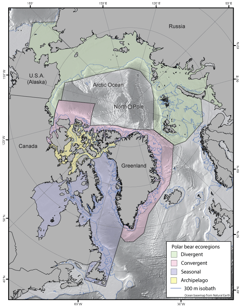
Polar bear (Ursus maritimus) ecoregions (Divergent, Convergent, Seasonal, and Archipelago) as defined by Amstrup and others (2008) and used by Durner and others (2009) and Atwood and others (2016). Map is shown in a polar stereographic projection (EPSG:3411, https://epsg.io/3411). Ocean map with benthic relief from Natural Earth (2022; https://naturalearthdata.com).
Methods
All CMIP model outputs were downloaded in NetCDF format (Unidata, 2022; https://www.unidata.ucar.edu/software/netcdf/) from data nodes hosted by the Earth System Grid Federation (2022; https://esgf.llnl.gov/) and coordinated by the World Climate Research Program (2022; https://www.wcrp-climate.org/). Specifically, for models listed in table 1, we obtained monthly sea-ice concentration (SIC) simulations from both CMIP5 (accessed May 2013) and CMIP6 (accessed November 2020) based on the historical forcing experiment, as well as 21st century projections based on three CMIP5 forcing scenarios (RCP26, RCP45, and RCP85) and three CMIP6 scenarios (SSP126, SSP245, and SSP585). For CMIP5 models, 2005 was the first year of 21st century scenario-based projections, while for CMIP6 models that year was 2015. For all models and forcing experiments, we obtained “run 1” when multiple model runs were available.
Table 1.
List of Coupled Model Intercomparison Project Phase 5 (CMIP5) and CMIP6 Earth systems models used in this study, including the models’ origin country and institute, and basis for selection.[ECS (equilibrium climate sensitivity) and TCR (transient climate response): Values from Meehl and others (2020). Abbreviations: °C, degrees Celsius; W, Wang and Overland (2015); M, Massonnet and others (2012); S, SIMIP Community (2020); --, values not reported]
The 13 CMIP5 models used in this study (table 1) are the same as those used by Atwood and others (2016). They were selected from among dozens of models in the CMIP5 archive based on criteria defined by Massonnet and others (2012) and Wang and Overland (2012, 2015). Wang and Overland (2015) identified 12 models that simulated means and seasonal cycles in ice extent to within 20 percent of observations, while Massonnet and others (2012) identified six models based also on comparisons with observed means and seasonal cycles, as well as metrics based on ice volume and September trend. Together, the two studies identified 15 unique models, of which we excluded 2 lower-resolution models (IPSL-CM5A-LR and MPI-ESM-LR) because their medium-resolution counterparts (IPSL-CM5A-MR and MPI-ESM-MR) were included.
For CMIP6, we used a subset of models based on selection criteria defined by SIMIP Community (2020) that retained a model if its ensemble spread among historical simulations included the observed 2005–2014 September mean sea-ice area and the observed change in sea-ice area for a given change in cumulative anthropogenic CO2 during 1979–2014. The purpose of these criteria was to select a subset of models for estimating a best guess of the future evolution of the Arctic sea-ice cover (SIMIP Community, 2020). Thirteen models were selected by SIMIP Community (2020, table S4), but we excluded HadGEM3-GC31-LL because its medium-resolution counterpart (HadGEM3-GC31-MM) was included; hence, 12 CMIP6 models were used in this study (table 1).
Observational data of monthly SIC, derived from passive microwave satellite remote sensing imagery of the northern hemisphere spanning 1979–2020, were obtained from the National Snow and Ice Data Center (Cavalieri and others, 1996). This dataset was designed to provide a consistent time series of observed sea-ice concentrations spanning the coverage of several passive microwave instruments. The data were provided in polar stereographic projection with a grid cell size of 25 × 25 kilometers (km).
The CMIP SIC data were disseminated in model-specific non-uniform ocean grids, so we reprojected and resampled the data onto the same polar stereographic grid as the sea-ice observations using nearest-neighbor assignments to preserve the ESMs’ native resolution.
All data summaries described below were applied to each ESM, under each forcing experiment, for each month, and within each of the 4 polar bear ecoregions (fig. 1) as described and named by Amstrup and others (2008). The single time series of observational SIC data was treated similarly. Data summaries for the Archipelago Ecoregion excluded five CMIP5 ESMs and three CMIP6 ESMs (table 1) with such coarse spatial resolution that many of the region’s major fjords were unresolved and depicted as land. This is not to imply, however, that the ESMs we included in the Archipelago Ecoregion summaries adequately represent the region’s complex topography. It could be argued that all contemporary ESMs lack sufficient spatial resolution to simulate the region’s nuanced oceanography (McGeehan and Maslowski, 2012) and that dismissing ESM sea-ice projections altogether for the Archipelago Ecoregion is warranted (Molnár and others, 2020).
For each monthly SIC grid, we calculated the area within each polar bear ecoregion that was covered by sea ice with greater than or equal to 15 percent concentration (in other words, ice extent). Next, because different ESMs depicted land masses slightly differently, we calculated the proportion (expressed as a percentage) of a given ecoregion that was ice-covered by dividing the area of ice extent by the ecoregion’s model-specific total pelagic area. We plotted the proportions as time series of 10-year running averages over the 21st century and visually highlighted the CMIP5 with CMIP6 multimodel means.
We repeated the calculations above but using a greater than or equal to 50 percent SIC threshold for defining ice extent and within just the continental shelf areas (less than 300 meters [m] depth) of each ecoregion. When the proportion of continental shelf covered by greater than or equal to 50 percent SIC fell below 50 percent during a given month, that month was classified as “ice-free.” This term “ice-free” is meant to describe a month as having reduced or diminished polar bear habitat and not necessarily a complete absence of sea ice. The 50 percent thresholds were specifically chosen due to their relationships with polar bear habitat (Durner and others, 2009) and their specific use in the Bayesian network models of Amstrup and others (2008) and Atwood and others (2016). Similarly, we plotted projected ice-free months as 10-year running averages over the 21st century and visually compared CMIP5 with CMIP6 by including their multimodel means. While a growing number of CMIP models have disseminated daily output data which could provide more resolved estimates of the ice-free period, we used monthly data in this study to maintain continuity with Atwood and others (2016).
We calculated model-specific relative changes in ice-free months by subtracting a given model’s mean number of ice-free months per year during the earliest decade of data (2015–2024) from the model’s mean number at mid-century (2045–2054) and at century’s end (2090–2099). We calculated these changes for each model relative to itself because different ESMs possess unique model configurations that produce a spread of multimodel uncertainty, including potential biases (Giorgi, 2010; Latif, 2011). We compared projected ice-free month changes between the CMIP5 and CMIP6 models by assuming equivalency in the paired RCP and SSP emissions scenarios (in other words, the 2.6, 4.5, and 8.5 W/m2 end-of-century pathways). We graphed the comparisons, by ecoregion, decade, and emissions scenario, as box plots and put summary statistics into tables.
We also estimated the annual total number of ice-free months at mid-century and end-of-century by extrapolating each model’s projected change from above (expressed as an annual rate) forward in time, starting from the satellite-observed average number of ice-free months during the most recent decade (2011–2020) and ending 35 years later using the mid-century rate and 80 years later using the end-of-century rate. Applying model-specific relative changes to fixed baseline values reduced influences from model biases. We compared the total ice-free month estimates derived from CMIP5 and CMIP6 models by ecoregion, decade, and emissions scenario with box plots and tabled statistics.
We used variance components analysis with each month’s total ice cover (by ecoregion and for early, mid, and late century) to estimate the proportion of variance attributable for four factors: (1) CMIP generations (CMIP5 and CMIP6); (2) forcing scenarios (2.6, 4.5 and 8.5 W/m2); (3) models; and (4) remainder, presumably incorporating natural variability in the Earth’s climate system as simulated by the models. Since we only used one run from each model and scenario (“run-1”), the variance component depicting natural variability is indirectly estimated by partitioning out other sources. We used Program R version 4.1.0 (R Core Team, 2021) and the “fitVCA” function with an “anova” option from the package “VCA” (Schuetzenmeister and Dufey, 2020). The method assigned zero to any negative variance component estimate and excluded its contribution to the total variance.
Results
Model Selections
The selected model subsets had slightly higher ECS and TCR overall than the unselected models across both CMIP generations (fig. 2). Importantly, the selected model subsets for both CMIP5 and CMIP6 maintained a broad representation of the full multimodel spread. The outcomes of model selection were generally similar between CMIP5 and CMIP6 with respect to ECS and TCR. This reduced concerns that the different model selection criteria (Massonnet and others, 2012; Wang and Overland, 2015; SIMIP Community, 2020) may have introduced biases that could have otherwise invalidated further comparisons. Also, the selected CMIP6 models as an ensemble had slightly higher ECS and TCR values than the selected CMIP5 models (fig. 2), which indicates that the CMIP6 subset likely would tend to project slightly more sea-ice loss in the future, on average, especially under higher GHG forcing during the latter 21st century (Tebaldi and others, 2021).
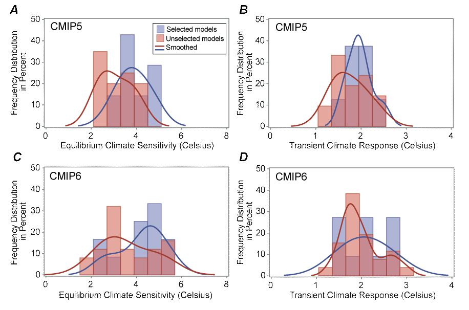
Frequency distributions of equilibrium climate sensitivity (ECS, left) and transient climate response (TCR, right) for selected (blue) and unselected (red) models from the Coupled Model Intercomparison Project Phase 5 (CMIP5) (A, B) and CMIP6 (C, D) model generations. ECS and TCR values from Meehl and others (2020). Selected models are listed in table 1.
Time-Series Comparisons
The monthly observed and model-projected sea-ice time series (fig. 3; app. 1, figs. 1.1–1.4) shared several general patterns that were common across all ecoregions: (1) observed sea ice declined during almost all months; (2) models projected continuing sea-ice declines over the 21st century; (3) forcing scenarios with higher GHG emissions resulted in greater sea-ice loss; (4) projections by individual ESMs varied widely within emissions scenario; (5) differences between emissions scenarios were relatively small through mid-century but very large by century’s end; and (6) the CMIP5 and CMIP6 multimodel averages showed considerable temporal congruency (within emissions scenario), with the exception of the Archipelago Ecoregion during summer (figs. 3H, 1.4). Overall, CMIP6 models tended to project slightly less ice cover, on average, than CMIP5 models across all emissions scenarios and in most months, especially toward century’s end.
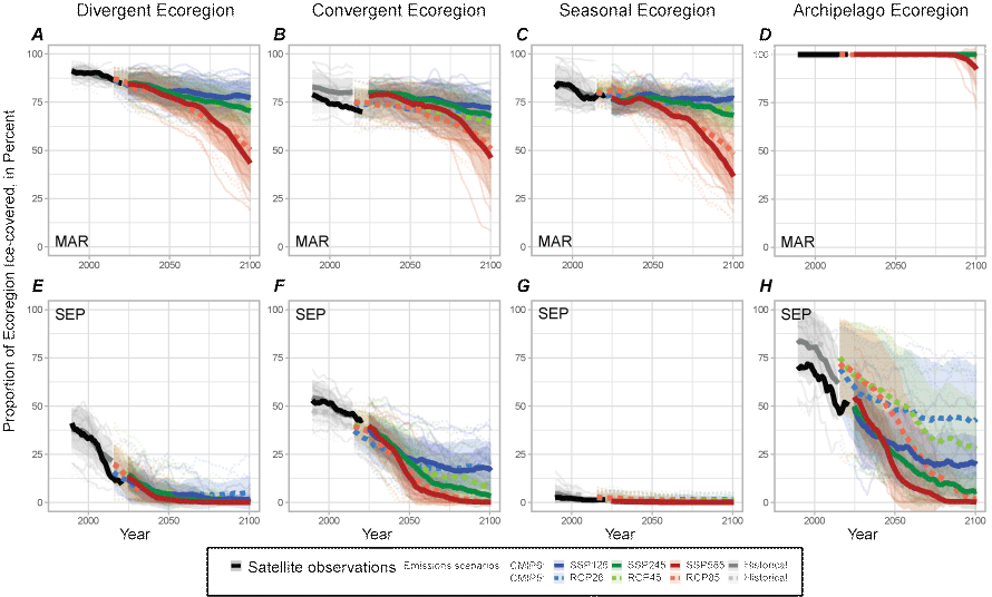
Percentage of four polar bear (Ursus maritimus) ecoregions (Divergent, Convergent, Seasonal, Archipelago; fig. 1) covered by sea ice (greater than 15 percent ice concentration) in March (A, B, C, D ) and September (E, F, G, H) as recorded by satellite observations (black line), as simulated (historical forcing) for recent decades by selected Coupled Model Intercomparison Project Phase 5 (CMIP5, broken lines) and CMIP6 (solid lines) models (table 1) through 2004 and 2014 (gray lines), and as projected through 2100 when forced by different greenhouse gas emissions scenarios (colored lines) named “representative concentration pathways (RCP; CMIP5)” and “shared socioeconomic pathways (SSP; CMIP6).” Bold gray and colored lines are multimodel averages shaded by ±1 standard deviation (sd); all lines plot 10-year running means. Analogous graphs for all months of the year are presented in figs. 1.1–1.4.
Given the criteria used to select the model subsets, we expected a reasonable degree of continuity (in other words, alignment) between recent observations of sea ice and the earliest model projections of future sea ice. In the Divergent Ecoregion, both CMIP5 and CMIP6 exhibited a high degree of continuity in the transition between recent sea-ice observations and the averaged multimodel near-term projections (figs. 3A, 3E, 1.1). That is, the bold black lines (observations) aligned reasonably well with the bold colored lines (model projections) in fig. 1.1. The most notable exception in continuity was during summer when the projected rate of near-term sea-ice loss did not keep pace with the recent observed rate of loss, sensu “faster than forecast” (Stroeve and others, 2007). Model averages for both the CMIP5 and CMIP6 ensembles projected complete ice loss during July–November under the high emissions scenario by century’s end, while CMIP6 projected slightly less ice than CMIP5 during the remaining months (fig. 1.1).
In the Convergent Ecoregion, during December–May, continuity between recent sea-ice observations and averaged ice projections was better among CMIP5 models than CMIP6 models, which were biased high in terms of sea-ice loss (figs. 3B, 1.2). That pattern reversed in July–October, however, when CMIP6 models were better aligned with observations, and CMIP5 model averages were low by comparison. Nevertheless, by mid-century and beyond, congruencies between the CMIP5 and CMIP6 model averages in the Convergent Ecoregion were generally similar, as in the Divergent Ecoregion (figs. 1.1, 1.2). Model averages for the CMIP5 and CMIP6 ensembles projected complete ice loss during August–October under the high emissions scenario by the end of the century (fig. 1.2).
In the Seasonal Ecoregion, recent ice observations and near-term model projections showed reasonable continuity for both CMIP averages in most months, except notably in December when recent observations showed a pause in ice decline, but the model-projected trajectories continued with an uninterrupted downward trend (fig. 1.3). Congruencies between CMIP5 and CMIP6 projections over time were like those in Divergent and Convergent ecoregions. CMIP5 and CMIP6 model-averaged ensembles projected complete ice loss under the high emissions scenario during July–November by the end of the century (fig. 1.3).
Recent observations show that the Archipelago Ecoregion was entirely ice-covered from November through May (fig. 1.4). This is the only ecoregion to retain 100 percent ice cover because, unlike other ecoregions, it does not include a peripheral sea that remains partially ice-covered in winter (such as the Barents, Greenland, and Bering seas). All models projected that the Archipelago Ecoregion will remain completely ice-covered during December–May until century’s end, except under the highest GHG emissions scenario. Models projected notable ice declines during summer and autumn (July–November) as also evidenced in the observational data. However, a lack of congruency between CMIP5 and CMIP6 projections in the Archipelago Ecoregion during summer months was readily evident (fig. 1.4). On average, in the Archipelago Ecoregion during summer, CMIP6 models projected more prominent ice loss than CMIP5 models under all three emissions scenarios. In August and September, the CMIP6 average near-term ice projections showed good continuity with recent rates of observed ice loss while the CMIP5 averages were biased high, suggesting some improved skill among models in the CMIP6 subset for this ecoregion.
Variance Components
Different sources of uncertainty (in other words, variability) in sea-ice projections contributed differently over the course of the 21st century (fig. 4). The foremost pattern, common to all ecoregions, was that variability attributable to the different emissions scenarios was negligible through mid-century but dominant by century’s end. A second prominent pattern was that variability attributable to the CMIP model generation was minor through mid-century and negligible by century’s end. For example, in the Divergent Ecoregion during 2020–2029 (fig. 4A), the dominant source of variability across all months was attributable to models, followed by natural climate variability which explained most of the remaining variance, while that attributable to the CMIP generation was very small and to emission scenarios negligible. The same patterns generally prevailed in mid-century (2045–2054), with the model contributions increasing slightly while the CMIP contribution diminished entirely. During 2090–2099 in the Divergent Ecoregion (fig. 4C), variability attributable to emission scenarios dominated in all months except August–September when consensus was attained among all scenarios that the region would become nearly ice-free (fig. 1.1).
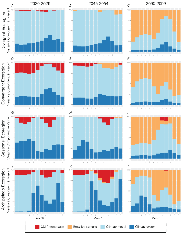
Components of the total monthly variability in the proportions of four polar bear (Ursus maritimus) ecoregions covered by sea ice (greater than 15 percent ice concentration) during each of three decadal periods (early, mid, and late century) as projected by multimodel ensembles (table 1) when forced with different greenhouse gas emissions scenarios. The graphed variance components show the estimated amount of variation in sea-ice cover attributable to four sources of variability: (1) the two generations of Coupled Model Intercomparison Project Phase models (CMIP5 and CMIP6), (2) three emission scenarios nested with the CMIP generation (that is, end-of-century net increases of 2.6 watts per square meter [W/m2], 4.5 W/m2, and 8.5 W/m2), (3) climate models (table 1) nested within scenario, and (4) the remaining variance presumably representing natural variability in the Earth’s climate system as simulated by the models.
In the Convergent Ecoregion, variability attributable to the CMIP model generation was greater than in other ecoregions during 2020–2029 (fig. 4D). During this decade, the CMIP6 models tended to project more ice cover than CMIP5, especially during winter months (fig. 1.2). But by mid-century (fig. 4E), CMIP variability was relatively small, and became negligible by late century (fig. 4F).
In the Seasonal Ecoregion, in late winter during 2020–2029 (fig. 4G), a small proportion of variability was attributable to the CMIP generations, but it did not persist into the mid or late century (figs. 4H, 4I). During summer in the Seasonal Ecoregion, interpretations of variance components are not informative because the region is effectively ice-free throughout the century under all scenarios (fig. 1.3), so the variance is small and mostly noise. Similarly, in the Archipelago Ecoregion, variance components are not informative during months and periods when the entire region is projected to be completely ice-covered (fig. 1.4). In the Archipelago Ecoregion, the most notable variance attributable to CMIP generation occurred during summer months in the early- and mid-21st century (figs. 4J, 4K) and stemmed from the CMIP6 models projecting less ice than CMIP5 models (fig. 1.4), together with an unknown degree of influence by models with different land masks and spatial resolutions. Different model land masks would be much less influential in the other three ecoregions because they are much larger than the Archipelago Ecoregion and have much larger ocean areas.
Ice-Free Months
The annual number of ice-free months was projected to increase in all ecoregions over the 21st century (fig. 5). Transition between recent observations and near-term multimodel averages showed good continuity in the Divergent Ecoregion for both CMIP5 and CMIP6 models (fig. 5A) and good continuity for CMIP6 in the Convergent Ecoregion (fig. 5B). In the Seasonal Ecoregion, the upward trends projected for the near-term by the multimodel averages did not transition well with the recent observed trend which had flattened considerably over the past decade (fig. 5C). In the Archipelago Ecoregion, transition between observations and projections was better aligned with the CMIP6 model average than with CMIP5 (fig. 5D). The CMIP5 models underestimated recent observations compared to CMIP6 in the Archipelago Ecoregion and projected consistently fewer ice-free months throughout the century (fig. 5D), a pattern described earlier for the ice cover time series (fig. 1.4).
![Annual number of ice-free months for shelf waters (less than 300 meters [m] deep)
within four polar bear ecoregions (Divergent, Convergent, Seasonal, Archipelago; fig.
1) as recorded by satellite observations since 1979 (black line), as simulated (historical
forcing) in recent decades by Coupled Model Intercomparison Project Phase 5 (CMIP5,
broken lines) and CMIP6 (solid lines) models (table 1) through 2004 or 2014 (gray
lines), and as projected through 2100 when forced by different greenhouse gas emissions
scenarios (colored lines). An ‘ice-free month’ was counted when the spatial extent
of sea ice having greater than 50 percent concentration covered less than 50 percent
of an ecoregion’s shelf waters. Bold gray and colored lines are multimodel averages
shaded by ±1 standard deviation (sd); all lines plot 10-year running means.](https://pubs.usgs.gov/of/2022/1062/images/ofr20221062_fig05.png)
Annual number of ice-free months for shelf waters (less than 300 meters [m] deep) within four polar bear ecoregions (Divergent, Convergent, Seasonal, Archipelago; fig. 1) as recorded by satellite observations since 1979 (black line), as simulated (historical forcing) in recent decades by Coupled Model Intercomparison Project Phase 5 (CMIP5, broken lines) and CMIP6 (solid lines) models (table 1) through 2004 or 2014 (gray lines), and as projected through 2100 when forced by different greenhouse gas emissions scenarios (colored lines). An ‘ice-free month’ was counted when the spatial extent of sea ice having greater than 50 percent concentration covered less than 50 percent of an ecoregion’s shelf waters. Bold gray and colored lines are multimodel averages shaded by ±1 standard deviation (sd); all lines plot 10-year running means.
Before midcentury, rates of increase in ice-free months were similar among all emissions scenarios (fig. 5), but after midcentury rates: (1) accelerated under the high (8.5 W/m2) emissions scenario; (2) continued somewhat uniformly under the intermediate (4.5 W/m2) scenario; and (3) flattened under the low (2.6 W/m2) emissions scenario.
Nearly all ESMs projected that the average annual number of ice-free months in 2045–2054 (and 2090–2099) will increase relative to the mean number projected for 2015–2024 in all ecoregions and under all forcing scenarios (fig. 6A, 6B). A dominant pattern throughout fig. 6 is the considerable amount of overlap between the CMIP5 and CMIP6 models, except during late century in the Divergent and Seasonal Ecoregions under the two higher emissions scenarios when CMIP6 models show a tendency to project slightly more ice-free months per year compared to the CMIP5 models.
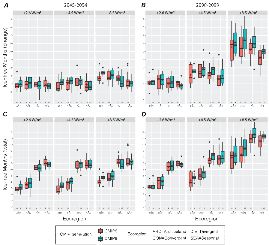
Change in the number of ice-free months at mid-century (A, 2045–2054) and at century’s end (B, 2090–2099), relative to the most contemporary decade (2015–2024), as projected by ensembles of Coupled Model Intercomparison Project Phase 5 (CMIP5, red) and CMIP6 (blue) models (table 1) when forced by different greenhouse gas emission scenarios. CMIP5 models were forced with ‘RCP’ scenarios (RCP26, RCP45, and RCP85), and CMIP6 models with ‘SSP’ scenarios (SSP126, SSP245, and SSP585), and both are graphed under headings of their respective end-of-century net increase in radiative forcing (+2.6 watts per square meter [W/m2], +4.5 W/m2, and +8.5 W/m2). Annual total number of ice-free months for mid-century (C, 2045–2054) and century’s end (D, 2090–2099) as projected by the same models and scenarios as in the top row. Box-and-whisker notation shows the multimodel mean (plus symbol), median (horizontal line), interquartile range (IQR, shaded box), ±1.5 IQR (whiskers), and outliers (dots). Sample sizes (n models in the ensemble) are shown below each box plot. See tables 2 and 3 for tabulated values.
Because continued ice loss was curbed under the low emissions scenario during the second half of the 21st century, changes in the number of ice-free months at century’s end were largely the same as midcentury (figs. 6A, 6B), which was also reflected by the flattened slopes in the low emission time series of fig. 5. Similarly, the generally constant slopes of the intermediate scenario (fig. 5) corresponded with an approximate doubling of ice-free months from mid to late century, while the accelerated rates associated with the high emissions scenario resulted in a three to fourfold increase in ice-free months over the second half of the century (fig. 6A, 6B).
We applied the ice-free month changes shown in fig. 6A and 6B to the 2011–2020 average ice-free months from observations to estimate the total annual number of ice-free months in each ecoregion at mid- and late-century (fig. 6C, 6D). The observed ice-free months during 2011–2020 (in other words, the baseline values) in the Archipelago, Convergent, Divergent, and Seasonal ecoregions averaged, 2.0, 2.5, 5.3, and 6.0 months. Not surprisingly, there were consistently more total ice-free months per year in the Seasonal and Divergent ecoregions compared to the Convergent and Archipelago ecoregions (fig. 6C, 6D). Dominant patterns in fig. 6C and 6D parallel the partitioning of variance components shown in fig. 4. For example, during midcentury, the data distributions across all three emissions scenarios (fig. 6C) were very similar, consistent with the small contribution of emission scenario to the total variance at midcentury (fig. 4B, 4E, 4H, 4F). In contrast, during late century, the data distributions were markedly different across scenarios (fig. 6D), consistent with the large contribution of emissions scenario to the total variance at that time (fig. 4C, 4F, 4I, 4L).
Discussion
Uncertainties in projections of Arctic sea ice over the 21st century come primarily from the wide spread of outputs by different models, and the wide range of conceivable emissions scenarios the world might follow (SIMIP Community, 2020; Bourdeau-Goulet and Hassanzadeh, 2021). In contrast, the degree of uncertainty introduced by differences in the CMIP model generation (specifically CMIP5 and CMIP6) is small and diminishes over time (fig. 4). Studies that have compared observations to large multimodel ensembles of CMIP5 and CMIP6 simulations have reported that “performances of CMIP6 and CMIP5 models are very similar in the representations of sea-ice extent seasonal cycle and long-term trend for both hemispheres” (Shu and others, 2020); and “we find that there is little difference in overall model performance between CMIP3, CMIP5 and CMIP6. The multimodel spread of the mean quantities remains large, the observational record lies within the multimodel ensemble spread, and many models simulate plausible values of mean sea-ice area when considering the impact of internal variability and observational uncertainty” (SIMIP Community, 2020). This is not to imply, however, that CMIP5 and CMIP6 models produce identical outputs, especially at regional scales and seasonal timeframes. For example, Long and others (2021) found that CMIP6 models had large positive biases in sea-ice concentration around the Barents and East Greenland seas during winter, which may have contributed to the positive biases we found for CMIP6 in the Convergent Ecoregion during winter compared to observations (fig. 1.2).
Expectations that simulations of sea ice by ESMs should precisely match observations are unreasonable. As much as 50 percent of the recent observed loss of summer sea ice has been attributed to internal (natural) variability that manifests nonuniformly over the Arctic (England and others, 2019; Watts and others, 2021). Multimodel averages often tend to have better agreement with observations, for reasons that are not entirely clear (Reichler and Kim, 2008). If different models produce unbiased outputs that vary somewhat evenly about the truth, then averaging would serve to remove noise arising not only from the simulation of natural variability, but probably to a larger extent from the uncertainties attributable to different model formulations (Reichler and Kim, 2008; Pierce and others, 2009). While many of the multimodel averages in our regional-scale summaries exhibited good agreement with observations, some did not (figs. 5, 1.1–1.4). When agreement was lacking, the CMIP5 and CMIP6 averages often shared a common offset, possibly indicating a systemic bias among the models (for example, October in the Divergent Ecoregion, fig. 1.1). As noted earlier, the Convergent Ecoregion was an area where disagreements between models and observations were different for the two CMIP generations in terms of ice cover: CMIP5 models simulated observations better during winter months while CMIP6 models were better during summer (fig. 1.2). Modest amounts of disagreement between observations and simulations should not, however, discount a model’s usefulness since stricter agreement with observations is not a guarantee for more reliable projections (Knutti and others, 2010).
Because radiative forcing among the emissions scenarios evolved similarly until about 2040 (Moss and others, 2010; O'Neill and others, 2016), sea-ice projections across scenarios also were similar until then (figs. 1.1–1.4), and scenarios contributed relatively little to the total variability through midcentury (fig. 4). But by century’s end, the dominant source of uncertainty had switched to emissions scenarios (fig. 4) because sea-ice projections (and radiative forcing) began diverging markedly after 2040 (figs. 1.1–1.4). Not knowing now which emissions trajectory society will more closely follow over the 21st century imparts a very high degree of uncertainty about Earth’s future climate and emphasizes that the most important factor controlling the future is societal choice. Like most assessments using CMIP projections, we have assumed the emissions scenarios to be equally probable, although likelihood of the highest scenario (8.5 W/m2) has generated debate (Grant and others, 2020; Hausfather and Peters, 2020; Schwalm and others, 2020; Natali and others, 2021).
Sea-ice variability attributable to the two generations of CMIP models was minor through midcentury and negligible by century’s end, relative to the other sources of uncertainty considered (fig. 4). Nevertheless, we found modest, non-zero differences between CMIP5 and CMIP6 models in their projected changes to ice-free months (table 2).
Table 2.
Average and median change in the number of ice-free months, in continental shelf waters, from the most contemporary decade (2015–2024) to either midcentury (2045–2054) or to century’s end (2090–2099) as projected by multimodel ensembles of Coupled Model Intercomparison Project Phase 5 (CMIP5) and CMIP6 models (table 1) when forced by different greenhouse gas emissions scenarios in each of four polar bear (Ursus maritimus) ecoregions (fig. 1).[Abbreviations: sd, standard deviation; n, number of models; min, minimum; max, maximum]
Table 3.
Average and median total number of ice-free months per year, in continental shelf waters, estimated for midcentury (2045–2054) and century’s end (2090–2099) as projected by multimodel ensembles of Coupled Model Intercomparison Project Phase 5 (CMIP5) and CMIP6 models (table 1) when forced by different greenhouse gas emissions scenarios.[Abbreviations: sd, standard deviation; n, number of models; min, minimum; max, maximum]
Would such minor differences in the CMIP6 sea-ice projections be sufficient to substantively change the polar bear population outcome states derived by the Bayesian network model of Atwood and others (2016) which used CMIP5 sea-ice projections? Given the high degree of overall congruence between CMIP5 and CMIP6 models in their projected sea-ice cover over time and across ecoregions (figs. 1.1–1.4), and relatively small differences in their projected ice-free month changes (table 2), evidence suggests it is unlikely that using CMIP6 model outputs would qualitatively change the results and interpretations presented by Atwood and others (2016). We reached this conclusion by considering the Bayesian network’s construct, including how sea-ice input nodes were binned, and how those binned values were integrated with other nodes through conditional probability tables (Atwood and others 2015). We provide some examples below to contextualize our reasoning.
The Bayesian network by Atwood and others (2016) included three sea-ice input nodes that were populated with values derived from CMIP5 projections: (1) changes in ice-free months; (2) total annual area of optimal ice habitat; and (3) distance between the ice pack and shelf waters during the sea-ice minimum in just the Divergent and Convergent ecoregions; and a fourth subjectively populated node named “foraging sea-ice quality” that captured expert knowledge about how seasonal changes in sea-ice availability would affect polar bear habitat quality. Our evaluation of the Bayesian network model here focuses on the ice-free months variable because not only has duration of the ice-free season been shown to directly correlate with polar bear condition, but it is also a reasonable surrogate for the two other sea-ice inputs. As ice-free months diminish, the annual area of optimal habitat decreases, and retreat of the summer ice pack increases.
Sea-ice metrics were derived as continuous values representing decadal averages, but upon input into the Bayesian network, they were binned into five or six categorical levels (detailed in Atwood and others, 2015). For example, the change in ice-free months (the “IceChng” node in Atwood and others, 2015) was binned into six intervals based on whole integer assignments: less than 0, 0, 1, 2, 3–4, and 5 or more. Binning the raw input values into categories diminishes that node’s sensitivity to small numerical changes. Consider the 12 pairs of late-century (2090–2099) CMIP5–CMIP6 mean ice-free month comparisons shown in table 2 (one comparison for each of 3 emissions scenarios, across 4 ecoregions). Eleven of the 12 comparisons involve pairs with identical whole (truncated) integer values, meaning that upon entry into the Bayesian network they would be binned into the same categorical level. In other words, for these 11 cases, using the ice-free month values derived from CMIP6 models in the Bayesian network would be indistinguishable from using CMIP5 values because the binning would create equivalency.
The one exception among the 12 comparisons described above was in the Seasonal Ecoregion under the high emissions scenario: the CMIP5 and CMIP6 mean values were 4.1 and 5.0 ice-free months, so they would be binned differently–into the input node’s 3–4 and the 5-or-more month categories. The significance of the 5-or-more month category is that adverse population-level effects, including near total failure of cub recruitment, are expected when bears must fast for greater than 5 months (Robbins and others, 2012, Molnár and others, 2020; Pilfold and others, 2016). The ramifications of the difference in binning can be assessed by examining the conditional probability table that joined the “IceChng” input node with the “IceShelf” input node (see fig. 3 and table E4 in Atwood and others, 2015). Switching from the 3–4-month category (CMIP5 models) to the 5-or-more category (CMIP6 models) would change the prescribed probabilities for the foraging habitat availability states (“IceFor” node) from 10 percent reduced and 90 percent greatly reduced (for the 3–4-month input) to 100 percent greatly reduced (for the 5-or-more month input). That minor (10 percent net) change in the state probabilities for foraging habitat availability would then be assimilated when the “IceFor” node is integrated with two other nodes via another conditional probability table that determines the states likelihoods that comprise the overall “Ice” node (table E3 in Atwood and others, 2015). Before reaching the final “population status” node of the Bayesian network (fig. 3 in Atwood and others, 2015), the overall “Ice” node states pass through four to six more conditional probability tables that serve to assimilate other types of potential stressors to polar bears such as prey abundance, pollution, disturbance, hunting, and disease.
The conditional probability tables that comprise the polar bear Bayesian network of Atwood and others (2016) were prescribed by applying gradients of probability across the range of categorical outcome states, which typically represented relationships of relative magnitude like “more, less, or the same.” Such generalized categories would tend to buffer, rather than amplify, modest changes to input node values as they propagate through the many intermediate nodes and conditional probability tables toward the final output node–“population state.”
Differences between the CMIP5 and CMIP6 sea-ice projections were most apparent during July–October in the Archipelago Ecoregion (fig. 1.4). Nevertheless, since ice-free months was calculated as a relative change for each ESM, differences between the CMIP5 and CMIP6 averages at the end of the century were small (table 2) and would be negated by the binning during input to the Bayesian network (as described above). At midcentury, however, changes in ice-free months by CMIP6 models would enter the Bayesian network slightly higher than the CMIP5 models for the intermediate and high emissions scenarios (table 2). Those increases would likely manifest in the Bayesian network as a slight improvement to the polar bear population outcome states in the Archipelago Ecoregion at midcentury. Atwood and others (2016) specifically prescribed that improvement (via the conditional probability tables) because the expert panel agreed that “thinning of the multiyear ice may actually improve the quality of foraging sea-ice habitat.” However, at century’s end in the Archipelago, despite no differences between CMIP5 and CMIP6 ice-free month changes after binning (table 2), the greater extent of summer ice melt projected by CMIP6 models during summer (fig. 1.4) would likely cause the network’s final polar bear population outcomes to have slightly higher end-of-century probabilities in the decreased and greatly decreased states.
Conclusions
Consistent with other comparisons of sea-ice outputs by different CMIP model generations (SIMIP Community, 2020), we found only modest differences between selected CMIP5 and CMIP6 model subsets in their projections of ice cover within four polar bear ecoregions. Greater sources of variability among sea-ice projections stem from differences between models and between GHG emissions scenarios. We thus hypothesize that using sea-ice projections from CMIP6 models instead of CMIP5 in the Bayesian network of Atwood and others (2016), while holding all other inputs and model structures the same, would not cause qualitative changes to interpretations of polar bear population outcomes across ecoregions and emissions scenarios reported therein. Three factors support that inference: (1) differences between CMIP5 and CMIP6 ice projections were relatively small on average (figs. 5, 6, 1.1–1.4; table 2); (2) binning the sea-ice inputs into categorical states would remove most minor differences between CMIP5 and CMIP6 upon entry; and (3) prescribed gradients in the network’s numerous conditional probability tables would tend to dilute small changes to the sea-ice input states as they propagated toward the final output node.
References Cited
Amstrup, S.C., Marcot, B.G., and Douglas, D.C., 2008, A Bayesian network modeling approach to forecasting the 21st century worldwide status of polar bears, in DeWeaver, E.T., Bitz, C.M., and Tremblay, L-B., eds., Arctic Sea ice decline—Observations, projections, mechanisms, and implications: Geophysics Monograph Series, v. 180, p. 213–268, American Geophysical Union, Washington, D.C., accessed January 29, 2009, at https://doi.org/10.1029/180GM14.
Amstrup, S.C., DeWeaver, E.T., Douglas, D.C., Marcot, B.G., Durner, G.M., Bitz, C.M., and Bailey, D.A., 2010, Greenhouse gas mitigation can reduce sea-ice loss and increase polar bear persistence: Nature, v. 468, no. 7326, p. 955–958, accessed December 15, 2010, at https://doi.org/10.1038/nature09653.
Andrews, T.J.M., Gregory, J.M., Webb, M.J., and Taylor, K.E., 2012, Forcing, feedbacks and climate sensitivity in CMIP5 coupled atmosphere–ocean climate models: Geophysical Research Letters, v. 39, no. 9, L09712, accessed December 27, 2021, at https://doi.org/10.1029/2012GL051607.
Atwood, T.C., Marcot, B.G., Douglas, D.C., Amstrup, S.C., Rode, K.D., Durner, G.M., and Bromaghin, J.F., 2015, Evaluating and ranking threats to the long-term persistence of polar bears: U.S. Geological Survey Open-File Report 2014–1254, 124 p., accessed January 13, 2015, at https://doi.org/10.3133/ofr20141254.
Atwood, T.C., Marcot, B.G., Douglas, D.C., Amstrup, S.C., Rode, K.D., Durner, G.M., and Bromaghin, J.F., 2016, Forecasting the relative influence of environmental and anthropogenic stressors on polar bears: Ecosphere, v. 7, no. 6, p. e01370, accessed July 5, 2016, at https://doi.org/10.1002/ecs2.1370.
Bourdeau-Goulet, S.-C., and Hassanzadeh, E., 2021, Comparisons between CMIP5 and CMIP6 models: Simulations of climate indices influencing food security, infrastructure resilience, and human health in Canada: Earth's Future, v. 9, e2021EF001995, accessed January 6, 2022, at https://doi.org/10.1029/2021EF001995.
Caldwell, P.M., Zelinka, M.D., Taylor, K.E., and Marvel, K., 2016, Quantifying the sources of intermodel spread in equilibrium climate sensitivity: Journal of Climate, v. 29, no. 2, p. 513–524, accessed December 26, 2021, at https://doi.org/10.1175/JCLI-D-15-0352.1.
Cavalieri, D.J., Parkinson, C.L., Gloersen, P., and Zwally, H.J., 1996 updated yearly, sea ice concentrations from Nimbus-7 SMMR and DMSP SSM/I-SSMIS passive microwave data, version 1: Monthly northern hemisphere data, National Snow and Ice Data Center, Boulder, Colorado, accessed July 21, 2021, at ftp://sidads.colorado.edu.
Charney, J.G., Arakawa, A., Baker, D.J., Bolin, B., Dickinson, R.E., Goody, R.M., Leith, C.E., Stommel, H.M., and Wunsch, C.I., 1979, Carbon dioxide and climate—A Scientific Assessment: Washington, DC, USA, The National Academies Press, 34 p., accessed December 28, 2021, at https://doi.org/10.17226/12181.
Durner, G.M., Douglas, D.C., Nielson, R.M., Amstrup, S.C., McDonald, T.L., Stirling, I., Mauritzen, M., Born, E.W., Wiig, Ø., DeWeaver, E., Serreze, M.C., Belikov, S.E., Holland, M.M., Maslanik, J., Aars, J., Bailey, D.A., and Derocher, A.E., 2009, Predicting 21st-century polar bear habitat distribution from global climate models: Ecological Monographs, v. 79, no. 1, p. 25–58, accessed February 20, 2009, at https://doi.org/10.1890/07-2089.1.
Earth System Grid Federation, 2022, What is ESGF?: Earth System Grid Federation, accessed June 9, 2022, at https://esgf.llnl.gov/.
Edwards, P.N., 2011, History of climate modeling: Wiley Interdisciplinary Reviews: Climate Change, v. 2, no. 1, p. 128–139, accessed December 22, 2021, at https://doi.org/10.1002/wcc.95.
England, M., Jahn, A., and Polvani, L., 2019, Nonuniform contribution of internal variability to recent Arctic sea ice loss: Journal of Climate, v. 32, no. 13, p. 4039–4053, accessed January 7, 2022, at https://doi.org/10.1175/JCLI-D-18-0864.1.
Eyring, V., Bony, S., Meehl, G.A., Senior, C.A., Stevens, B., Stouffer, R.J., and Taylor, K.E., 2016, Overview of the Coupled Model Intercomparison Project Phase 6 (CMIP6) experimental design and organization: Geoscientific Model Development, v. 9, no. 5, p. 1937–1958, accessed December 28, 2021, at https://doi.org/10.5194/gmd-9-1937-2016.
Giorgi, F., 2010, Uncertainties in climate change projections, from the global to the regional scale—European Physical Journal (EPJ): Web of Conferences, v. 9, p. 115–129, accessed December 31, 2021, at https://doi.org/10.1051/epjconf/201009009.
Grant, N., Hawkes, A., Napp, T., and Gambhir, A., 2020, The appropriate use of reference scenarios in mitigation analysis: Nature Climate Change, v. 10, no. 7, p. 605–610, accessed January 9, 2022, at https://doi.org/10.1038/s41558-020-0826-9.
Hausfather, Z., and Peters, G.P., 2020, Emissions–The “business as usual” story is misleading: Nature, v. 577, no. 7792, p. 618–620, accessed January 9, 2022, at https://doi.org/10.1038/d41586-020-00177-3.
Hunter, C.M., Caswell, H., Runge, M.C., Regehr, E.V., Amstrup, S.C., and Stirling, I., 2010, Climate change threatens polar bear populations—A stochastic demographic analysis: Ecology, v. 91, no. 10, p. 2883–2897, accessed March 17, 2011, at https://doi.org/10.1890/09-1641.1.
Intergovernmental Panel on Climate Change [IPCC], 2007, Climate change 2007—Synthesis report—Contribution of Working Groups I, II and III to the Fourth Assessment Report of the Intergovernmental Panel on Climate Change [Core Writing Team, Pachauri, R.K and Reisinger, A. (eds.)]. IPCC, Geneva, Switzerland, p. 104, accessed March 3, 2015, at https://www.ipcc.ch/reports/.
Intergovernmental Panel on Climate Change [IPCC], 2014Climate change 2014—Synthesis report—Contribution of Working Groups I, II and III to the Fifth Assessment Report of the Intergovernmental Panel on Climate Change [Core Writing Team, R.K. Pachauri and L.A. Meyer (eds.)]: IPCC, Geneva, Switzerland, p. 151, accessed March 3, 2015, at https://www.ipcc.ch/reports/.
Intergovernmental Panel on Climate Change [IPCC], 2022, ipcc—The Intergovernmental Panel on Climate Change, accessed June 9, 2022, at https://www.ipcc.ch/.
Intergovernmental Panel on Climate Change [IPCC], in progress, 2022, AR6 Synthesis Report: Climate Change 2022, accessed January 6, 2022, at https://www.ipcc.ch/reports/.
Knutti, R., and Hegerl, G.C., 2008, The equilibrium sensitivity of the Earth’s temperature to radiation changes: Nature Geoscience, v. 1, no. 11, p. 735–743, accessed December 26, 2021, at https://doi.org/10.1038/ngeo337.
Knutti, R., Reinhard, F., Tebaldi, C., Cermak, J., and Meehl, G.A., 2010, Challenges in combining projections from multiple climate models: Journal of Climate, v. 23, no. 10, p. 2739–2758, accessed January 7, 2022, at https://doi.org/10.1175/2009JCLI3361.1.
Knutti, R., Rugenstein, M., and Hegerl, G., 2017, Beyond equilibrium climate sensitivity: Nature Geoscience, v. 10, no. 10, p. 727–736, accessed December 28, 2021, at https://doi.org/10.1038/ngeo3017.
Latif, M., 2011, Uncertainty in climate change projections: Journal of Geochemical Exploration, v. 110, no. 1, p. 1–7, accessed December 31, 2021, at https://doi.org/10.1016/j.gexplo.2010.09.011.
Long, M., Zhang, L., Hu, S., and Qian, S., 2021, Multi-aspect assessment of CMIP6 models for Arctic sea ice simulation: Journal of Climate, v. 34, no. 4, p. 1515–1529, accessed January 6, 2022, at https://doi.org/10.1175/JCLI-D-20-0522.1.
Marcot, B.G., 2012, Metrics for evaluating performance and uncertainty of Bayesian network models: Ecological Modelling, v. 230, p. 50–62, accessed March 29, 2022, at https://doi.org/10.1016/j.ecolmodel.2012.01.013.
Massonnet, F., Fichefet, T., Goosse, H., Bitz, C.M., Philippon-Berthier, G., Holland, M.M., and Barriat, P.-Y., 2012, Constraining projections of summer Arctic Sea ice: The Cryosphere, v. 6, no. 6, p. 1383–1394, accessed June 23, 2015, at https://doi.org/10.5194/tc-6-1383-2012.
McGeehan, T., and Maslowski, W., 2012, Evaluation and control mechanisms of volume and freshwater export through the Canadian Arctic Archipelago in a high-resolution pan-Arctic ice-ocean model: Journal of Geophysical Research, v. 117, C00D14, accessed December 31, 2021, at https://doi.org/10.1029/2011JC007261.
Meehl, G.A., Covey, C., Delworth, T., Latif, M., McAvaney, B., Mitchell, J.F.B., Stouffer, R.J., and Taylor, K.E., 2007, The WCRP CMIP3 multimodel dataset–A new era in climate change research: Bulletin of the American Meteorological Society, v. 88, no. 9, p. 1383–1394, accessed December 28, 2021, at https://doi.org/10.1175/BAMS-88-9-1383.
Meehl, G.A., Senior, C.A., Eyring, V., Flato, G., Lamarque, J.-F., Stouffer, R.J., Taylor, K.E., and Schlund, M., 2020, Context for interpreting equilibrium climate sensitivity and transient climate response from the CMIP6 Earth system models: Science Advances, v. 6, eaba1981, accessed November 19, 2021, at https://doi.org/10.1126/sciadv.aba1981.
Molnár, P.K., Bitz, C.M., Holland, M.M., Kay, J.E., Penk, S.R., and Amstrup, S.C., 2020, Fasting season length sets temporal limits for global polar bear persistence: Nature Climate Change, v. 10, no. 8, p. 732–738, accessed July 21, 2020, at https://doi.org/10.1038/s41558-020-0818-9.
Moss, R.H., Edmonds, J.A., Hibbard, K.A., Manning, M.R., Rose, S.K., Van Vuuren, D.P., Carter, T.R., Emori, S., Kainuma, M., Kram, T., Meehl, G.A., Mitchell, J.F.B., Nakicenovic, N., Riahi, K., Smith, S.J., Stouffer, R.J., Thomson, A.M., Weyant, J.P., and Wilbanks, T.J., 2010, The next generation of scenarios for climate change research and assessment: Nature, v. 463, no. 7282, p. 747–756, accessed January 9, 2022, https://doi.org/10.1038/nature08823.
Nakicenovic, N., Alcamo, J., Davis, G., de Vries, H.J.M., Fenhann, J., Gaffin, S., Gregory, K., Grubler, A., Jung, T.Y., Kram, T., La Rovere, E.L., Michaelis, L., Mori, S., Morita, T., Papper, W., Pitcher, H., Price, L., Riahi, K., Roehrl, A., Rogner, H.H., Sankovski, A., Schlesinger, M., Shukla, P., Smith, S., Swart, R., van Rooijen, S., Victor, N., and Dadi, Z., 2000, Special report on emissions scenarios—A special report of Working Group III of the Intergovernmental Panel on Climate Change: Cambridge, United Kingdom, and New York, N.Y., Cambridge University Press, p. 570, accessed December 20, 2021, at https://www.grida.no/publications/120.
Natali, S.M., Holdren, J.P., Rogers, B.M., Treharne, R., Duffy, P.B., Pomerance, R., and MacDonald, E., 2021, Permafrost carbon feedbacks threaten global climate goals: Proceedings of the National Academy of Sciences of the United States of America, v. 118, no. 21, p. e2100163118, accessed March 31, 2022, at https://doi.org/10.1073/pnas.2100163118.
Natural Earth, 2022, Free vector and raster map data at 1:10m, 1:50m, and 1:11m scales: Natural Earth, accessed June 17, 2022, at https://www.naturalearthdata.com/.
Nijsse, F.J.M.M., Cox, P.M., and Williamson, M.S., 2020, Emergent constraints on transient climate response (TCR) and equilibrium climate sensitivity (ECS) from historical warming in CMIP5 and CMIP6 models: Earth System Dynamics: ESD, v. 11, no. 3, p. 737–750, accessed November 19, 2021, at https://doi.org/10.5194/esd-11-737-2020.
Notz, D., 2015, How well must climate models agree with observations?: Philosophical Transactions—Royal Society. Mathematical, Physical, and Engineering Sciences, v. 373, no. 2052, p. 20140164, accessed January 6, 2022, at https://doi.org/10.1098/rsta.2014.0164.
O’Neill, B.C., Tebaldi, C., Van Vuuren, D.P., Eyring, V., Friedlingstein, P., Hurtt, G., and Sanderson, B.M., 2016, The Scenario Model Intercomparison Project (ScenarioMIP) for CMIP6: Geoscientific Model Development, v. 9, no. 9, p. 3461–3482, accessed January 6, 2022, at https://doi.org/10.5194/gmd-9-3461-2016.
Pierce, D.W., Barnett, T.P., Santer, B.D., and Gleckler, P.J., 2009, Selecting global climate models for regional climate change studies: Proceedings of the National Academy of Sciences of the United States of America, v. 106, no. 21, p. 8441–8446, accessed May 31, 2012. https://doi.org/10.1073/pnas.0900094106.
Pilfold, N.W., Hedman, D., Stirling, I., Derocher, A.E., Lunn, N.J., and Richardson, E., 2016, Mass lost rates of fasting polar bears: Physiological and Biochemical Zoology, v. 89, no. 5, p. 377–388, accessed July 21, 2020, at https://doi.org/10.1086/687988.
R Core Team, 2021, R: A Language and Environment for Statistical Computing, Vienna, Austria, accessed November 13, 2021, at https://www.R-project.org/.
Reichler, T., and Kim, J., 2008, How well do coupled models simulate today’s climate?: Bulletin of the American Meteorological Society, v. 89, no. 3, p. 303–312, accessed December 28, 2022, at https://doi.org/10.1175/BAMS-89-3-303.
Robbins, C.T., Lopez-Alfaro, C., Rode, K.D., Tøien, Ø., and Nelson, O.L., 2012, Hibernation and seasonal fasting in bears—The energetic costs and consequences for polar bears: Journal of Mammalogy, v. 93, no. 6, p. 1493–1503, accessed July 21, 2020, at https://doi.org/10.1644/11-MAMM-A-406.1.
Rugenstein, M., Bloch-Johnson, J., Gregory, J., Andrews, T., Mauritsen, T., Li, C., Frölicher, T.L., Paynter, D., Danabasoglu, G., Yang, S., Dufresne, J.-L., Cao, L., Schmidt, G.A., Abe-Ouchi, A., Geoffroy, O., and Knutti, R., 2020, Equilibrium climate sensitivity estimated by equilibrating climate models: Geophysical Research Letters, v. 47, no. 4, e2019GL083898, accessed December 28, 2021, at https://doi.org/10.1029/2019GL083898.
Schuetzenmeister, A., and Dufey, F., 2020, VCA—Variance component analysis, R package version 1.4.3, accessed December 14, 2021, at https://CRAN.R-project.org/package=VCA.
Schwalm, C.R., Glendon, S., and Duffy, P.B., 2020, RCP8.5 tracks cumulative CO2 emissions: Proceedings of the National Academy of Sciences of the United States of America, v. 117, no. 33, p. 19656–19657, accessed January 9, 2022, at https://doi.org/10.1073/pnas.2007117117.
Shen, Z., Duan, A., Dongliang, L., and Li, J., 2021, Assessment and ranking of climate models in Arctic sea ice cover simulation—From CMIP5 to CMIP6: Journal of Climate, v. 34, no. 9, p. 3609–3627, accessed December 17, 2021, at https://doi.org/10.1175/JCLI-D-20-0294.1.
Shu, Q., Wang, Q., Song, Z., Qiao, F., Zhao, J., Chu, M., and Li, X., 2020, Assessment of sea ice extent in CMIP6 with comparison to observations and CMIP5. Geophysical Research Letters, v 47, e2020GL087965, accessed October 12, 2021, at https://doi.org/10.1029/2020GL087965.
SIMIP Community, 2020, Arctic sea ice in CMIP6: Geophysical Research Letters, v. 47, e2019GL086749, accessed August 9, 2021, at https://doi.org/10.1029/2019GL086749.
Stroeve, J., Holland, M.M., Meier, W., Scambos, T., and Serreze, M., 2007, Arctic sea ice decline—Faster than forecast: Geophysical Research Letters, v. 34, no. 9, L09501, accessed May 29, 2010, at https://doi.org/10.1029/2007GL029703.
Taylor, K.E., Stouffer, R.J., and Meehl, G.A., 2012, An overview of CMIP5 and the experiment design: Bulletin of the American Meteorological Society, v. 93, no. 4, p. 485–498, accessed January 9, 2022, at https://doi.org/10.1175/BAMS-D-11-00094.1.
Tebaldi, C., Debeire, K., Eyring, V., Fischer, E., Fyfe, J., Friedlingstein, P., Knutti, R., Lowe, J., O’Neill, B., Sanderson, B., van Vuuren, D., Riahi, K., Meinshausen, M., Nicholls, Z., Tokarska, K.B., Hurtt, G., Kriegler, E., Lamarque, J.-F., Meehl, G., Moss, R., Bauer, S.E., Boucher, O., Brovkin, V., Byun, Y.-H., Dix, M., Gualdi, S., Guo, H., John, J.G., Kharin, S., Kim, Y., Koshiro, T., Ma, L., Olivié, D., Panickal, S., Qiao, F., Rong, X., Rosenbloom, N., Schupfner, M., Séférian, R., Sellar, A., Semmler, T., Shi, X., Song, Z., Steger, C., Stouffer, R., Swart, N., Tachiiri, K., Tang, Q., Tatebe, H., Voldoire, A., Volodin, E., Wyser, K., Xin, X., Yang, S., Yu, Y., and Ziehn, T., 2021, Climate model projections from the Scenario Model Intercomparison Project (ScenarioMIP) of CMIP6: Earth System Dynamics: ESD, v. 12, no. 1, p. 253–293, accessed January 6, 2022, at https://doi.org/10.5194/esd-12-253-2021.
Unidata, 2022, Network common data form: Unidata, accessed June 9, 2022, at https://www.unidata.ucar.edu/software/netcdf/.
U.S. Fish and Wildlife Service, 2008, Endangered and threatened wildlife and plants – Determination of Threatened Status for the polar bear (Ursus maritimus) throughout its range: Federal Register, v. 73, no. 95, p. 28211–28303, accessed December 20, 2021, at https://www.federalregister.gov/d/E8-11105.
U.S. Fish and Wildlife Service, 2016, Polar Bear (Ursus maritimus) Conservation Management Plan, Final: U.S. Fish and Wildlife Service, Region 7, Anchorage, Alaska, 104 p., accessed June 21, 2022, at https://ecos.fws.gov/docs/recovery_plan/PBRT%20Recovery%20Plan%20Book.FINAL.signed.pdf.
Wang, M., and Overland, J.E., 2009, A sea ice free summer Arctic within 30 years?: Geophysical Research Letters, v. 36, no. 7, L07502, accessed December 29, 2021, at https://doi.org/10.1029/2009GL037820.
Wang, M., and Overland, J.E., 2012, A sea ice free summer Arctic within 30 years—An update from CMIP5 models: Geophysical Research Letters, v. 39, no. 18, L18501, accessed December 29, 2021, at https://doi.org/10.1029/2012GL052868.
Wang, M., and Overland, J.E., 2015, Projected future duration of the sea-ice-free season in the Alaskan Arctic: Progress in Oceanography, v. 136, p. 50–59, accessed December 10, 2021, at https://doi.org/10.1016/j.pocean.2015.01.001.
Watts, M., Maslowski, W., Lee, Y.J., Kinney, J.C., and Osinski, R., 2021, A spatial evaluation of Arctic sea ice and regional limitations in CMIP6 historical simulations: Journal of Climate, v. 34, p. 6399–6420, accessed December 28, 2021, at https://doi.org/10.1175/JCLI-D-20-0491.1.
World Climate Research Programme, 2022, WCRP coupled model intercomparison project (CMIP): World Climate Research Program, accessed June 9, 2022, at https://www.wcrp-climate.org/wgcm-cmip.
Appendix 1. Observed and Model-Projected Sea-Ice Time Series
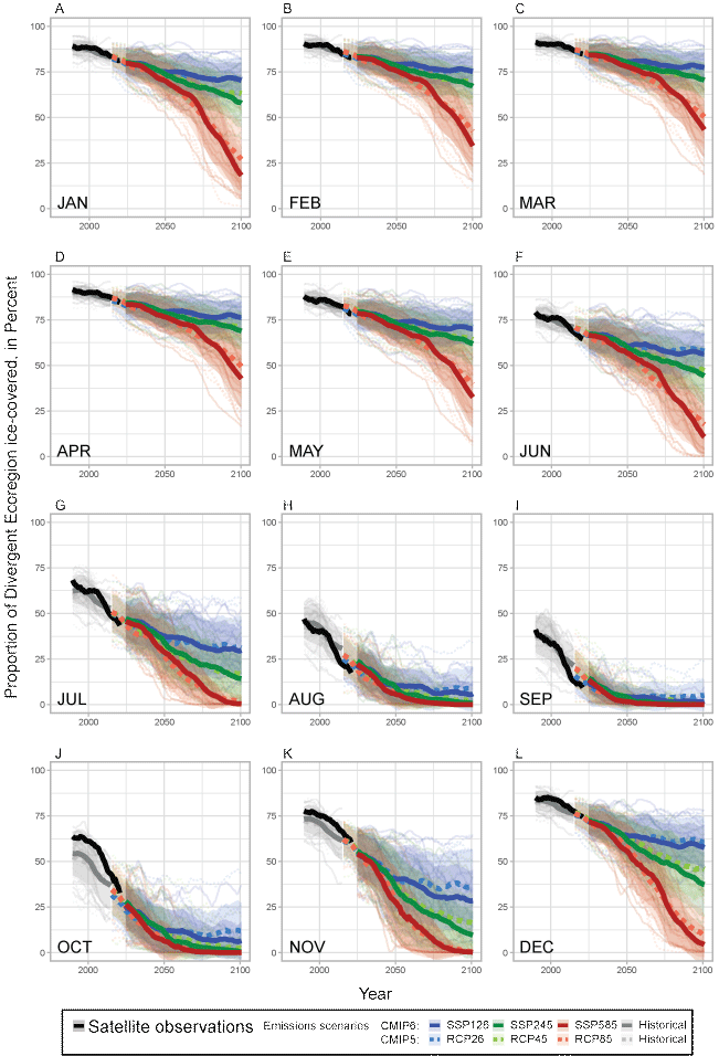
Monthly percentages of the Divergent Ecoregion (fig. 1) covered by sea ice (less than 15 percent ice concentration) as recorded by satellite observations since 1979 (black line), as simulated (historical forcing) in recent decades by Coupled Model Intercomparison Project Phase 5 (CMIP5, broken lines) and CMIP6 (solid lines) models (table 1) through 2004 and 2014, (gray lines), and as projected through 2100 when forced by different greenhouse gas emissions scenarios (colored lines) named “representative concentration pathways (RCP; CMIP5)” and “shared socioeconomic pathways (SSP; CMIP6).” Bold gray and colored lines are multimodel averages shaded by ±1 standard deviation (sd); all lines plot 10-year running means.
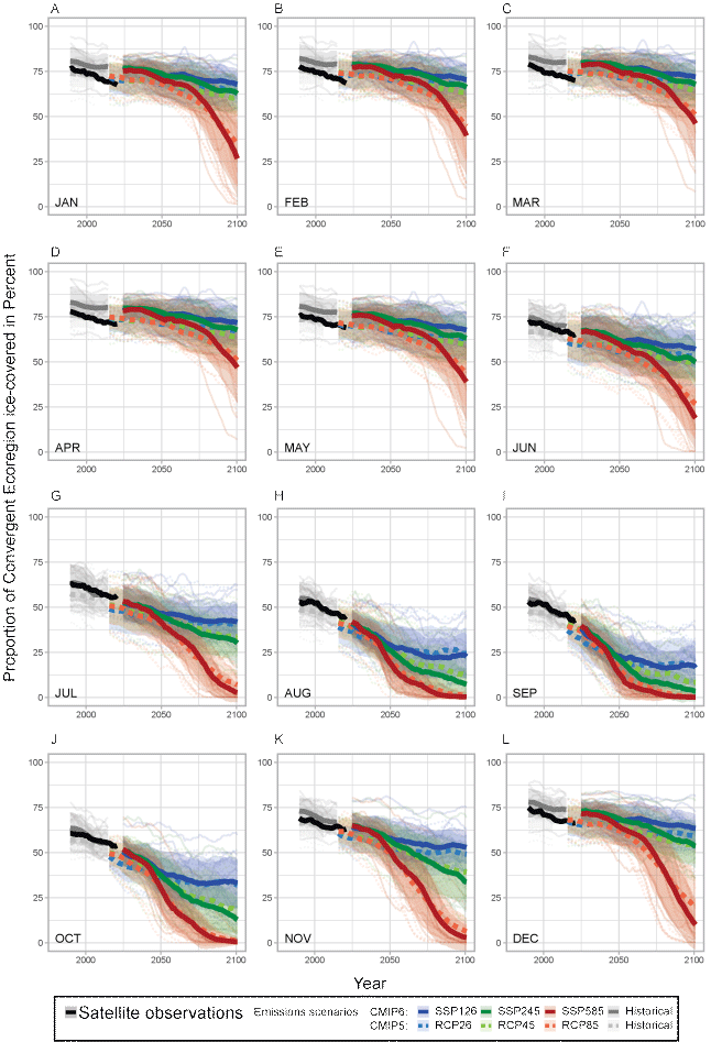
Monthly percentages of the Convergent Ecoregion (fig. 1) covered by sea ice (greater than 15 percent ice concentration) as recorded by satellite observations since 1979 (black line), as simulated (historical forcing) in recent decades by Coupled Model Intercomparison Project Phase 5 (CMIP5, broken lines) and CMIP6 (solid lines) models (table 1) through 2004 and 2014 (gray lines), and as projected through 2100 when forced by different greenhouse gas emissions scenarios (colored lines) named “representative concentration pathways (RCP; CMIP5)” and “shared socioeconomic pathways (SSP; CMIP6).” Bold gray and colored lines are multimodel averages shaded by ±1 standard deviation (sd); all lines plot 10-year running means.
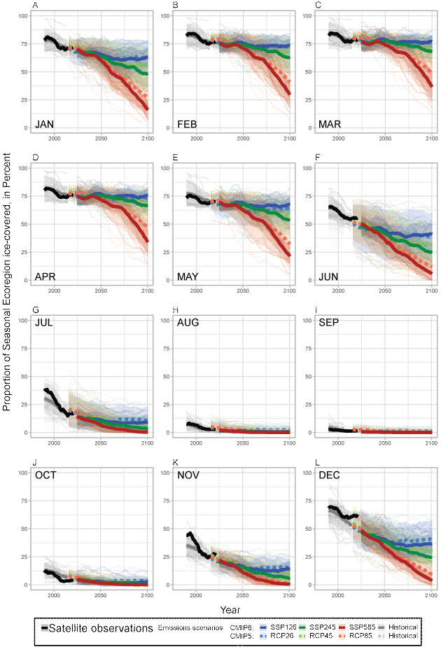
Monthly percentages of the Seasonal Ecoregion (fig. 1) covered by sea ice (less than 15 percent ice concentration) as recorded by satellite observations since 1979 (black line), as simulated (historical forcing) in recent decades by Coupled Model Intercomparison Project Phase 5 (CMIP5, broken lines) and CMIP6 (solid lines) models (table 1) through 2004 and 2014 (gray lines), and as projected through 2100 when forced by different greenhouse gas emissions scenarios (colored lines) named “representative concentration pathways (RCP; CMIP5)” and “shared socioeconomic pathways (SSP; CMIP6).” Bold gray and colored lines are multimodel averages shaded by ±1 standard deviation (sd); all lines plot 10-year running means.
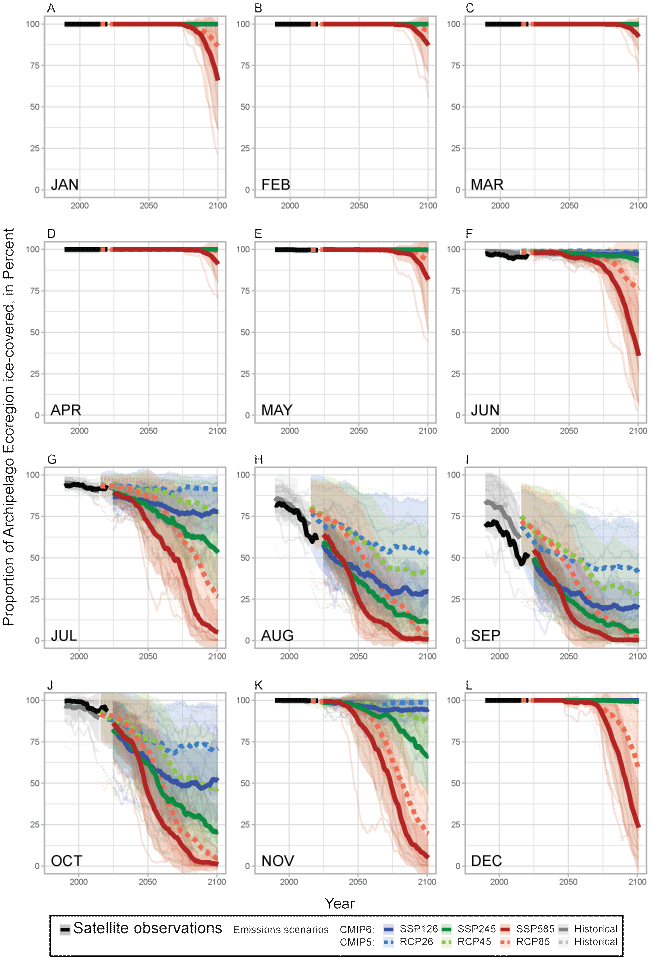
Monthly percentages of the Archipelago Ecoregion (fig. 1) covered by sea ice (greater than 15 percent ice concentration) as recorded by satellite observations since 1979 (black line), as simulated (historical forcing) in recent decades by Coupled Model Intercomparison Project Phase 5 (CMIP5, broken lines) and CMIP6 (solid lines) models (table 1) through 2004 and 2014 (gray lines), and as projected through 2100 when forced by different greenhouse gas emissions scenarios (colored lines) named “representative concentration pathways (RCP; CMIP5)” and “shared socioeconomic pathways (SSP; CMIP6).” Bold gray and colored lines are multimodel averages shaded by ±1 standard deviation (sd); all lines plot 10-year running means.
Table 1.1.
Coupled Model Intercomparison Project Phase 6 (CMIP6) models used in this study with data citations.| CMIP6 models | Data digital object identifier | Data citation |
|---|---|---|
| ACCESS-CM2 | https://doi.org/10.22033/ESGF/CMIP6.2285 | Dix and others (2019) |
| ACCESS-ESM1-5 | https://doi.org/10.22033/ESGF/CMIP6.2291 | Ziehn and others (2019) |
| CanESM5 | https://doi.org/10.22033/ESGF/CMIP6.1317 | Swart and others (2019) |
| CESM2-WACCM | https://doi.org/10.22033/ESGF/CMIP6.10026 | Danabasoglu (2019) |
| CNRM-ESM2-1 | https://doi.org/10.22033/ESGF/CMIP6.1395 | Seferian (2019) |
| EC-Earth3 | https://doi.org/10.22033/ESGF/CMIP6.251 | EC-Earth Consortium (2019a) |
| EC-Earth3-Veg | https://doi.org/10.22033/ESGF/CMIP6.727 | EC-Earth Consortium (2019b) |
| HadGEM3-GC31-MM | https://doi.org/10.22033/ESGF/CMIP6.10846 | Jackson (2020) |
| IPSL-CM6A-LR | https://doi.org/10.22033/ESGF/CMIP6.1532 | Boucher and others (2019) |
| MIROC6 | https://doi.org/10.22033/ESGF/CMIP6.898 | Shiogama and others (2019) |
| MRI-ESM2-0 | https://doi.org/10.22033/ESGF/CMIP6.638 | Yukimoto and others (2019) |
| NorESM2-LM | https://doi.org/10.22033/ESGF/CMIP6.604 | Seland and others (2019) |
References Cited
Boucher, O., Denvil, S., Levavasseur, G., Cozic, A., Caubel, A., Foujols, M.-A., Meurdesoif, Y., Cadule, P., Devilliers, M., Dupont, E., and Lurton, T., 2019, IPSL IPSL-CM6A-LR model output prepared for CMIP6 ScenarioMIP: Earth System Grid Federation, accessed November 19, 2020, at https://doi.org/10.22033/ESGF/CMIP6.1532.
Danabasoglu, G., 2019, NCAR CESM2-WACCM model output prepared for CMIP6 ScenarioMIP: Earth System Grid Federation, accessed November 11, 2020, at https://doi.org/10.22033/ESGF/CMIP6.10026.
Dix, M., Bi, D., Dobrohotoff, P., Fiedler, R., Harman, I., Law, R., Mackallah, C., Marsland, S., O’Farrell, S., Rashid, H., Srbinovsky, J., Sullivan, A., Trenham, C., Vohralik, P., Watterson, I., Williams, G., Woodhouse, M., Bodman, R., Dias, F.B., Domingues, C., Hannah, N., Heerdegen, A., Savita, A., Wales, S., Allen, C., Druken, K., Evans, B., Richards, C., Ridzwan, S.M., Roberts, D., Smillie, J., Snow, K., Ward, M., and Yang, R., 2019, CSIRO-ARCCSS ACCESS-CM2 model output prepared for CMIP6 ScenarioMIP: Earth System Grid Federation, accessed November 9, 2020, at https://doi.org/10.22033/ESGF/CMIP6.2285.
EC-Earth Consortium, 2019a, EC-Earth-Consortium EC-Earth3 model output prepared for CMIP6 ScenarioMIP: Earth System Grid Federation, accessed November 16, 2020, at https://doi.org/10.22033/ESGF/CMIP6.251.
EC-Earth Consortium, 2019b, EC-Earth-Consortium EC-Earth3-Veg model output prepared for CMIP6 ScenarioMIP: Earth System Grid Federation, accessed November 16, 2020, at https://doi.org/10.22033/ESGF/CMIP6.727.
Jackson, L., 2020, MOHC HadGEM3-GC31-MM model output prepared for CMIP6 ScenarioMIP: Earth System Grid Federation, accessed November 19, 2020, at https://doi.org/10.22033/ESGF/CMIP6.10846.
Seland, Ø., Bentsen, M., Oliviè, D.J.L., Toniazzo, T., Gjermundsen, A., Graff, L.S., Debernard, J.B., Gupta, A.K., He, Y., Kirkevåg, A., Schwinger, J., Tjiputra, J., Aas, K.S., Bethke, I., Fan, Y., Griesfeller, J., Grini, A., Guo, C., Ilicak, M., Karset, I.H.H., Landgren, O.A., Liakka, J., Moseid, K.O., Nummelin, A., Spensberger, C., Tang, H., Zhang, Z., Heinze, C., Iversen, T., and Schulz, M., 2019, NCC NorESM2-LM model output prepared for CMIP6 ScenarioMIP: Earth System Grid Federation, accessed November 22, 2020, at https://doi.org/10.22033/ESGF/CMIP6.604.
Seferian, R., 2019, CNRM-CERFACS CNRM-ESM2-1 model output prepared for CMIP6 ScenarioMIP: Earth System Grid Federation, accessed November 12, 2020, at https://doi.org/10.22033/ESGF/CMIP6.1395.
Shiogama, H., Abe, M., and Tatebe, H., 2019, MIROC MIROC6 model output prepared for CMIP6 ScenarioMIP: Earth System Grid Federation, accessed November 20, 2020, at https://doi.org/10.22033/ESGF/CMIP6.898.
Swart, N.C., Cole, J.N.S., Kharin, V.V., Lazare, M., Scinocca, J.F., Gillett, N.P., Anstey, J., Arora, V., Christian, J.R., Jiao, Y., Lee, W.G., Majaess, F., Saenko, O.A., Seiler, C., Seinen, C., Shao, A., Solheim, L., von Salzen, K., Yang, D., Winter, B., and Sigmond, M., 2019, CCCma CanESM5 model output prepared for CMIP6 ScenarioMIP: Earth System Grid Federation, accessed November 14, 2020, at https://doi.org/10.22033/ESGF/CMIP6.1317.
Yukimoto, S., Koshiro, T., Kawai, H., Oshima, N., Yoshida, K., Urakawa, S., Tsujino, H., Deushi, M., Tanaka, T., Hosaka, M., Yoshimura, H., Shindo, E., Mizuta, R., Ishii, M., Obata, A., and Adachi, Y., 2019, MRI MRI-ESM2.0 model output prepared for CMIP6 ScenarioMIP: Earth System Grid Federation, accessed November 21, 2020, at https://doi.org/10.22033/ESGF/CMIP6.638.
Ziehn, T., Chamberlain, M., Lenton, A., Law, R., Bodman, R., Dix, M., Wang, Y., Dobrohotoff, P., Srbinovsky, J., Stevens, L., Vohralik, P., Mackallah, C., Sullivan, A., O’Farrell, S., and Druken, K., 2019, CSIRO ACCESS-ESM1.5 model output prepared for CMIP6 ScenarioMIP: Earth System Grid Federation, accessed November 9, 2020, at https://doi.org/10.22033/ESGF/CMIP6.2291.
Conversion Factors
Datum
Horizontal coordinate information (as conveyed in fig. 1) is referenced to a polar stereographic projection with a datum based upon the Hughes 1980 ellipsoid (EPSG 3411, https://epsg.io/3411, accessed June 14, 2022).
Abbreviations
AR
Assessment Report
CMIP
Coupled Model Intercomparison Project
CMIP5
Coupled Model Intercomparison Project Phase 5
CMIP6
Coupled Model Intercomparison Project Phase 6
CO2
carbon dioxide
ECS
equilibrium climate sensitivity
ESM
earth system model
GHG
greenhouse gas
IPCC
Intergovernmental Panel on Climate Change
ppm
parts per million
RCP
representative concentration pathway
RCP26
Representative Concentration Pathway 2.6 (also, RCP45 and RCP85)
SIC
sea-ice concentration
SSP
shared socioeconomic pathway
SSP126
shared socioeconomic pathway 1-2.6 (also, SSP245 and SSP585)
TCR
transient climate response
USFWS
U.S. Fish and Wildlife Service
W/m2
watts per square meter
Publishing support provided by the U.S. Geological Survey
Science Publishing Network, Tacoma Publishing Service Center
For more information concerning the research in this report, contact the
Director, Alaska Science Center
U.S. Geological Survey
4210 University Drive
Anchorage, Alaska 99508
Suggested Citation
Douglas, D.C., and Atwood, T.C., 2022, Comparisons of Coupled Model Intercomparison Project Phase 5 (CMIP5) and Coupled Model Intercomparison Project Phase 6 (CMIP6) sea-ice projections in polar bear (Ursus maritimus) ecoregions during the 21st century: U.S. Geological Survey Open-File Report 2022–1062, 27 p., https://doi.org/10.3133/ofr20221062.
ISSN: 2331-1258 (online)
| Publication type | Report |
|---|---|
| Publication Subtype | USGS Numbered Series |
| Title | Comparisons of Coupled Model Intercomparison Project Phase 5 (CMIP5) and Coupled Model Intercomparison Project Phase 6 (CMIP6) sea-ice projections in polar bear (Ursus maritimus) ecoregions during the 21st century |
| Series title | Open-File Report |
| Series number | 2022-1062 |
| DOI | 10.3133/ofr20221062 |
| Year Published | 2022 |
| Language | English |
| Publisher | U.S. Geological Survey |
| Publisher location | Reston, VA |
| Contributing office(s) | Alaska Science Center Biology MFEB |
| Description | vii, 27 p. |
| Online Only (Y/N) | Y |
| Google Analytic Metrics | Metrics page |