

Using Seismic Noise Correlation to Determine the Shallow Velocity Structure of the Seattle Basin, Washington
Links
- Document: Report , HTML , XML
- Download citation as: RIS | Dublin Core
Acknowledgments
We thank the diligent people who permitted the sites, deployed and maintained the instruments, downloaded the data, and converted the data to SAC files for use: Doug Gibbons, Jon Connolly, and Nancy Sackman of the Pacific Northwest Seismic Network of the University of Washington and David Bowen, Tom Yelin, Adria McClain, Jacob Crummey, Patrick Bastien, Nick Stein, Josh Sessoms, and Marcos Alvarez of the U.S. Geological Survey (USGS). Alex Hutko (University of Washington) assembled the metadata and posted the data to the Incorporated Research Institutions for Seismology (IRIS) Data Management Center. We thank Keith Knudsen (USGS) for pointing out the availability of the USGS instruments. We thank Morgan Moschetti, Erin Wirth, and Bill Stephenson (USGS) for their helpful reviews. Data are available from the IRIS Data Management Center (https://www.iris.edu), under datasets GM.AB03-AB11, GM.AB13-AB.17, and UW.RAD1-RAD6. The computer programs for calculating group velocities from shear-wave velocity profiles were written by Robert Herrmann, St. Louis University (https://www.eas.slu.edu/eqc/eqcsoftware.html; Herrmann, 2013).
Abstract
Cross-correlation waveforms of seismic noise in the Seattle basin, Washington, were analyzed to determine the group velocities of surface waves and constrain the shear-wave velocity (VS) for depths less than about 2 kilometers (km). Twenty broadband seismometers were deployed for about 3 weeks in three dense arrays separated by about 5 km, with minimum intra-array station spacing of about 0.5 km. Cross correlations of only 9 days of noise recordings produced Green’s functions at periods of 2 to 6 seconds (s) for sites about 5 km apart. Usable noise correlations for shorter periods of 0.5 to 1.0 s were found for sites within the arrays separated by 1 to 2 km. We bandpass filtered the inter- and intra-array cross-correlation waveforms to determine Love-wave group velocities at periods of 0.5 to 6 s for paths within the Seattle basin and at 3 to 5 s for paths crossing the southern edge of the basin. We developed a non-linear inversion program to determine VS profiles that fit the observed group velocities for paths in the basin. We found that these group velocities are well fit by a variety of VS profiles, each with a distinct jump in VS at depths ranging from 0.9 to 1.3 km. This jump in VS is inferred to represent the top of bedrock. The observed group velocities are not matched by models with the top of bedrock at 0.7-km depth or shallower. The group velocities are also fit by a model with no large jumps in VS in depths less than 2.4 km. The VS profile for the middle of the basin from Stephenson and others (2017), with a depth to bedrock of 0.9 km, also adequately fits the group velocity observations, if a velocity gradient is added from 0.05- to 0.1-km depth. The results indicate that short (3-week) deployments of seismometers to record seismic noise may provide useful constraints on the VS of sedimentary basins.
Introduction
Accurate seismic velocity models are essential for making realistic synthetic seismograms that are appropriate for predicting ground-motion parameters and waveforms for future large earthquakes. In particular, accurate three-dimensional (3D) models of deep sedimentary basins are critical for assessing the seismic hazard to tall buildings in those basins (for example, Marafi and others, 2019).
The purpose of this study was to determine if a deployment of broadband seismometers for only 3 weeks in the Seattle basin, Washington, was sufficient to produce noise correlations that could be used to constrain the shallow shear-wave velocities (VS) in the Seattle basin. We found that noise recordings for a duration as short as 9 days were indeed useful for determining the VS for depths less than 2.0 kilometers (km).
Computer simulations of ground shaking in future large earthquakes rely on an accurate 3D model of seismic velocities and densities in the crust and upper mantle. Extensive 3D simulations were recently completed for moment magnitude (M) 9 earthquakes on the Cascadia subduction zone (Frankel and others, 2018; Wirth and others, 2018). Previously, 3D simulations for the Seattle basin were conducted for the M6.8 2001 Nisqually earthquake, other recorded local earthquakes, and hypothetical M6.5–7 earthquakes on the Seattle Fault (Frankel and Stephenson, 2000; Frankel and others, 2007, 2009; Wirth and others, 2019; Thompson and others, 2020).
Ground motions from the simulations exhibited substantial amplification of the Seattle and Tacoma basins, similar to that observed in recordings of local earthquakes, for periods of 1 to 10 seconds (s) (Frankel and others, 2018). It is especially important to have accurate models of these sedimentary basins at depths of 10 km and shallower to accurately predict their basin amplification (Frankel and others, 2018).
Stephenson and others (2017) constructed a 3D model for the Cascadia region used in the M9 simulations (denoted herein as SAO17) from a variety of seismological, geological, and geophysical data. The model for the Seattle basin consists of as much as 1.0 km of Quaternary sediments overlying as much as 6 km of Tertiary sedimentary rock, above volcanic basement rocks. The SAO17 model used the map of the thickness of the Quaternary sediments from Johnson and others (1999), which was determined from marine seismic reflection data and the Jones (1996) map of sediment thickness derived from limited borehole data.
The VS in the Quaternary sediments of the Seattle basin in the velocity model are not well constrained by previous data for depths greater than about 30 meters (m). The SAO17 model has the same VS with depth within the Quaternary sediments for all locations in the Seattle basin. The VS profiles from the surface to 30-m depth at several locations in the Seattle basin have been determined from seismic refraction studies (Williams and others, 1999; Stephenson, 2007) and surface-wave dispersion (Wong and others, 2011). The VS to 100-m depth were measured in two boreholes (Odum and others, 2004). As stated in Stephenson and others (2017), primary-wave velocities (VP) within the deep sediments of the Seattle basin were constrained by observations from marine seismic data in Puget Sound (Calvert and others, 2003). The SAO17 model was also informed by VS values for depths greater than 1 km determined from active seismic sources by Snelson and others (2007) for an east-west line in the Seattle basin about 2 km north of the study area of this paper. The SAO17 model used a VP/VS ratio that ranged from 2.5 to 2.2 from 0- to 1-km depth, respectively, to estimate the VS in the Quaternary sediments from the VP values.
Over the past 15 years or so, correlation of seismic noise between sites has been applied to determine VS structure on regional and local scales. This approach is based on the idea that the correlation of seismic noise between two sites represents the Green’s function or impulse response between the two sites (Lobkis and Weaver, 2001; Shapiro and Campillo, 2004). Delorey and Vidale (2011) used noise correlation and seismic tomography to determine the VS of the Seattle basin at depths less than 3.5 km. That study used a recording duration of a few months and found somewhat lower VS at depths of 1 to 3 km compared to the Stephenson (2007) model. However, the Delorey and Vidale (2011) study had limited resolution of VS at depths less than 1 km, and the tomographic inversion smoothed the VS contrast across the southern edge of the basin that is inferred from the surficial geology and observations of basin-edge generated surface waves (Frankel and others, 2002). More recently, Stephenson and others (2019) applied the spatially averaged coherency (SPAC) method to determine VS profiles to about 1.5-km depth in the Seattle basin. This method is based on fitting the shape of the coherency of seismic noise across a seismic array as a function of wavenumber. They found that increases in VS corresponding to the top of bedrock occurred at depths roughly comparable to those in the SAO17 model.
Empirical ground-motion models (GMM) that predict ground-shaking levels as a function of magnitude and distance often parameterize the amplification from deep sedimentary basins using the depths where the VS reaches 1.0 kilometer per second (km/s) (Z1.0) (for example, Chiou and Youngs, 2014) or 2.5 km/s (Z2.5). Z1.0 is generally assumed to be the depth to bedrock (Chiou and Youngs, 2014) and Z2.5 is taken to be the depth to crystalline basement rocks (Campbell and Bozorgnia, 2014). Thus, the depth to the top of bedrock is important for the prediction of ground shaking using empirical GMMs, as well as to 3D ground motion simulations.
In this study, useable Green’s functions were determined from noise correlations of stations separated by about 5 km after only 9 days of recording. These Green’s functions were analyzed to determine the group velocity of Love waves as a function of period from 0.5 to 6 s. We found that the SAO17 model, with a depth to bedrock of 0.9 km, was generally consistent with these group velocities. We developed an inversion program to find other VS profiles that matched the observed group velocities. These other models had depths to bedrock ranging from 0.9 to 1.3 km. Thus, the seismic noise data provided useful constraints on the near-surface VS and Z1.0 in the Seattle basin.
Data and Cross-Correlation Procedure
Three dense arrays totaling 20 broadband seismometers with digital recorders were deployed in Seattle, Wash., by personnel from the Pacific Northwest Seismic Network (University of Washington) and the U.S. Geological Survey (USGS). The instruments were operational for about 3 weeks in April and May 2017. Figure 1 is a map of the deployment with the arrays labeled NW (northwest), NE (northeast), and SE (southeast). Two of the arrays were located in the Seattle basin (NE, NW) and one (SE) was just to the south of the southern edge of the basin, as defined by geology and gravity (Blakely and others, 2002). The Seattle fault zone forms the southern boundary of the Seattle basin. Within each array, the stations had spacings of 0.5 to 1 km. The NE and SE arrays used compact Trillium sensors and the NW array consisted of Trillium 40 sensors. We removed instrument response before correlating recordings from different types of sensors. The original sampling interval was 0.01 s.
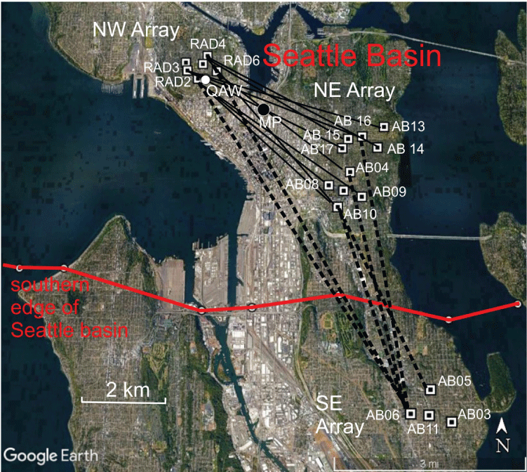
Map showing three dense seismic arrays used in this study, Seattle, Washington. Squares mark locations of broadband seismometers in the deployment. Black lines between stations indicate inter-array correlations used in this paper: solid lines are paths within Seattle basin, dashed lines are paths that cross southern edge of basin (red line). Southern edge of Seattle basin derived from gravity measurements (Richard Blakely, written comm., 2017). Black dot labeled MP is location of shear-wave velocity profile used in dispersion analysis. White dot is location of permanent station QAW of the Pacific Northwest Seismic Network. Unlabeled station symbols are stations that were not used in cross-correlation analysis because of timing problem or intermittent recording.
Cross correlations were calculated in the frequency domain for a set of consecutive time windows. We first decimated the seismograms to 10 samples per second. The horizontal seismograms were rotated into the transverse and radial components, relative to the path between the two stations. We initially tried one-bit normalization of the seismograms before cross correlation (see Bensen and others, 2007; Lin and others, 2008) but found it yielded similar cross correlations as the original non-normalized seismograms. The results shown here are from the original seismograms without normalization. We also tried pre-whitening the spectra of the waveforms but determined that this did not improve the results. For the inter-array correlations, we bandpass filtered the waveforms at 0.05 to 1 hertz (Hz) before cross correlation. For the intra-array correlations, a bandpass filter from 0.1 to 4 Hz was applied before correlating. Three stations were not used in the analysis because of a timing problem or intermittent recording (unlabeled symbols in fig. 1). Seismograms from 17 stations were analyzed in this study.
Cross-Correlation Results
Figure 2 shows that a 10-hour window of noise produces a correlation time series for two stations (RAD2 and AB09) 5 km apart with discernable pulses at 5- to 15-s positive and negative lag times. This is representative of the correlations of the transverse component between stations in the NW and NE arrays with paths entirely within the Seattle basin (fig. 1). We found consistent delay times of the peak of the correlated pulse for 10-hour windows over the duration of the deployment. The time series derived from stacking the correlation time series from 20 consecutive 10-hour windows (about 9 days) more clearly displays the pulses at 5- to 15-s positive and negative lag times (fig. 2). Positive lag time corresponds to waves propagating from northwest to southeast and negative lag time corresponds to waves traveling in the opposite direction. The results in this paper are based on stacking 20 consecutive 10-hour windows. Stacking additional windows did not substantially change the results. We did not include the period in the later part of the deployment when an ML 3.3 earthquake occurred on May 3, 2017, near Bremerton, Wash., about 25 km southwest of the NW array, so that signals from this earthquake did not affect the cross correlations. In general, we found different amplitudes for the pulses at positive and negative lag times. For any given cross correlation, we only used the pulse (positive or negative lag) with the largest amplitude for the dispersion analysis. We typically observed larger correlation pulses for paths travelling west to east across the basin, consistent with the seismic noise microseisms being preferentially generated to the west near the coast. Using the smaller amplitude pulses would not make a substantial difference to the results.
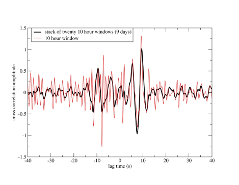
Plot of cross-correlation waveforms of seismic noise for stations RAD2 to AB09 for a 10-hour window and a stack of cross-correlation waveforms for 20 consecutive 10-hour windows. The transverse component of noise was used. s, seconds.
Figure 3 documents the moveout of the correlation pulse across stations in the NE array, indicating that the noise correlation represents the Green’s function of the path. These correlations use the same station in the NW array and three stations in the NE array. As the inter-station distance increases by about 1 km, the peak of the cross correlation is delayed by about 2 s. We conclude that these pulses on the correlation time series of the transverse time series represent the Love-wave impulse response between the two stations.
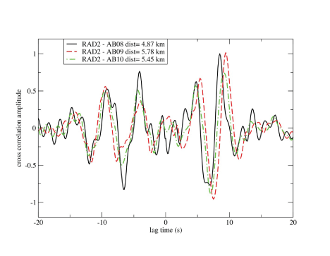
Plot of cross correlations of seismic noise using station pairs with increasing separation distances. Cross correlations exhibit moveout in time with increasing separation. Lag times at different periods of peak envelopes were used to calculate group velocities. Moveout of waveforms across the dense array was used to calculate phase velocity. The transverse component of noise was used. km, kilometers; s, seconds.
Cross correlation of the transverse components produced more distinct pulses compared to the correlations of the vertical and radial components. Figure 4 shows the clear pulses on the transverse correlation at 4- to 10-s positive lag and 3- to 12-s negative lag. Identifying pulses on the radial and vertical components was generally problematic for the waveforms we examined. This indicates that Love waves had higher correlations between sites than Rayleigh waves at the same period. Therefore, we restricted our analysis in this paper to the transverse component.
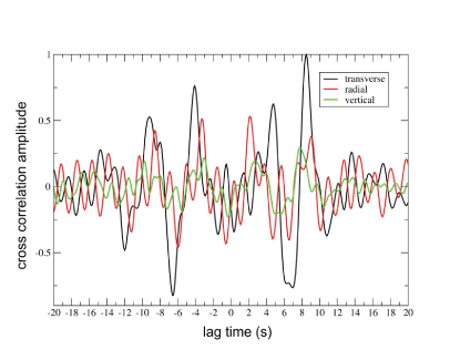
Plot of cross correlations of seismic noise at stations RAD2 and AB08, illustrating larger pulses on the transverse component compared to the radial and vertical components. s, seconds.
We determined group velocities of Love waves by bandpass filtering each cross-correlation waveform using zero-phase Butterworth filters, enveloping the filtered waveform, and picking the time of the peak amplitude of the envelope (Herrmann, 1973). Figure 5 exhibits the results of bandpass filtering the noise correlation waveform at 3- and 5-s periods, for two sites separated by about 5 km (RAD2 and AB08). The dispersion of the cross-correlation pulses is clearly indicated by the earlier arrival of the 5-s pulse compared to the 3-s pulse. Group velocities were determined by dividing the distance between the stations by the time delay of the peak of the envelope of the bandpass-filtered cross-correlation waveform.
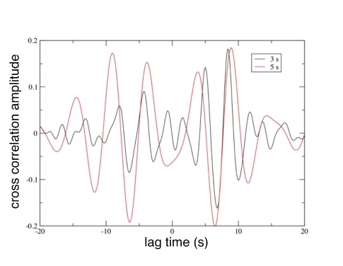
Plot of cross correlation of seismic noise at stations RAD2 and AB08, bandpass filtered at center periods of 3 and 5 seconds (s), illustrating faster group velocity at the longer period. The transverse component of noise was used.
There were several challenges in the cross-correlation analysis. For periods shorter than 2 s, there were generally no distinct pulses in the cross correlation for inter-array paths of about 5 km. At periods longer than about 6 s, the peak of the filtered waveform for the inter-array paths was too close to zero lag to be resolved in time. Theoretical studies recommend that the path be long enough such that the travel time is longer than the period (Tsai, 2009). The ratio of the delay time and maximum period of the waveforms in this study is comparable to that of the laboratory ultrasound study of Lobkis and Weaver (2001), who initially proposed the use of ambient noise correlation to determine Green’s functions.
Bandpass filtering the cross-correlation time series around a center period does not always produce a waveform that is predominantly at that center period. We chose center periods of 0.5, 1.0, 2.0, 3.0, 4.0, 5.0, and 6.0 s. The frequency width of the bandpass filters was 10 percent of the center frequency. The band-limited nature of the cross correlation caused by the dominant period of microseisms can make the dominant period of the filtered waveform lower than the center period specified in the filtering (Bensen and others, 2007). We calculated the dominant period of the filtered waveforms by measuring the time between zero crossings near the peak amplitude.
We calculated group velocities for 12 paths between the NW and NE arrays from 3 to 6 s periods and for 4 paths at 2 s (fig. 6). The station pairs have separation distances of about 5 km and are listed in table 1 and shown in figure 1. The average group velocity values for these inter-array measurements are plotted in figure 6 at the average periods of the bandpass-filtered cross-correlation waveforms. The error bars in figure 6 denote one standard deviation of the measurements for different pairs of stations. The other pairs of stations we examined yielded poor cross correlations and were not used in this study.
We also found usable cross correlations at 0.5- and 1.0-s periods for sites separated by about 1 to 2 km within the NE array. The group velocities at 0.5- and 1.0-s periods for five pairs of NE stations (intra-array paths) are also plotted in figure 6. We did not find usable cross correlations at these periods for stations within the NW and SE arrays.
The group velocities increase from about 0.42 km/s at a 0.5-s period to 0.72 km/s at about a 6-s period (fig. 6). In general, the standard deviations were larger for the shorter periods. The standard deviation in group velocities for a given period is likely caused by lateral variations in the VS depth profiles in the basin, as well as by measurement uncertainties.
We also cross correlated six paths crossing the southern edge of the Seattle basin (see table 1; fig. 1). These correlations were between stations in the NW and SE arrays and between stations in the NE and SE arrays. Figure 6 shows the average results found at 4- to 5-s periods. Shorter periods did not exhibit useful correlations. The group velocities for paths crossing the basin edge were about 1 km/s faster than those for the paths within the basin. This is expected because of the higher VS in the sedimentary rocks south of the basin edge compared to the glacial sediments in the basin at depths less than 1 km. We did not find useful cross correlations for inter-array paths with endpoints at AB11 or AB03 (fig. 1). These stations were located in an area of shallow bedrock (Tertiary sedimentary rock) which may have different noise characteristics. Cross correlations could be used for paths entirely outside the Seattle basin to quantify the VS in the rocks south of the basin.
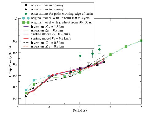
Plot of Love-wave group velocities measured from cross-correlation waveforms (data points with error bars of one standard deviation) and those calculated for the fundamental mode from flat-layered velocity models. m, meters; km, kilometers; Z1.0, depth to bedrock; VS, shear-wave velocity; km/s, kilometers per second; s, seconds.
Table 1.
Station pairs used to determine group velocities.[s, seconds]
Analysis of Group Velocities to Determine Shear-Wave Velocity Profiles
We compared the group velocities derived from the noise correlation for paths within the basin with those calculated for a flat-layered velocity model based on the SAO17 model, as well as other profiles. Love-wave group velocities for flat-layered velocity models were determined using the computer programs of Herrmann (2013). The layer thicknesses used correspond to those in the SAO17 model: 0.05-km thickness of the top layer, 0.1-km thickness to 1.3-km depth, and 0.3-km thickness from 1.3- to 10-km depth. The SAO17-model VS profile has a jump in VS at the base of the Quaternary sediments at 0.9-km depth (fig. 7). Tertiary sedimentary rock underlies the sediments. There is another distinct jump in VS at the top of the volcanic rock (basement) at about 7-km depth. The original SAO17 model had a minimum VS of 600 meters per second (m/s) for the top layer, based on the limitations of the 3D simulations. For the group velocity calculations, we lowered the VS in the top layer of the SAO17 model to 0.45 km/s, to be consistent with observations of near-surface VS on the glacial soils in the Seattle basin (Williams and others, 1999). We calculated densities from the VP in the SAO17 model using the empirical relationship given in Brocher (2005).
The SAO17 model at the midpoint of the arrays (MP in fig. 1) fits the observed group velocities except for at a 1-s period, where it was slightly larger than one standard deviation above the mean observed value (fig. 6). We found that introducing a VS gradient from 0.05- to 0.1-km depth improved the fit to the group velocity at a 1-s period. Thus, a minor modification of the SAO17 model matched the observed group velocities.
A key issue is the non-uniqueness of velocity profiles that fit the observed group velocities. To assess this non-uniqueness, we wrote a computer program to perform a nonlinear inversion of the observed group velocities to determine the VS for depths less than 2 km. Each iteration of the inversion determines the adjustments to the input VS profile that improve the fit to the observed group velocities. The program first finds the change in group velocity at each period given a perturbation in the VS for each layer. The group velocity at each period is calculated from the computer codes of Herrmann (2013). Damping and smoothing is also applied to stabilize the inversion. The inversion uses singular value decomposition to invert the matrix containing the derivatives of group velocity with respect to VS in each layer. The inversion program iterates until the root-mean-square error between the observed and predicted group velocities is no longer reduced significantly. The velocity in the top layer is constrained to be close to 0.45 km/s, based on the observed group velocity at a 0.5-s period.
Various VS profiles were found that adequately fit the observed group velocities from 0.5- to 6-s periods. Our suite of starting models had a constant velocity in the layers that were inverted for VS. Figure 7 contains the VS profiles from the SAO17 model and those from the inversions that fit the observed group velocities. The group velocities derived from the inversions are shown in figure 6. The starting VS profiles and the profiles determined from the inversions are displayed in figure 8. All of these profiles adequately fit the group velocity observations (fig. 6), with values within one standard deviation of the mean at each period.
For the first starting model, we solved for the VS in 14 layers at depths less than 2.0 km (fig. 8A). The layers have a thickness of 0.1 km to 1.3-km depth and 0.3 km for depths greater than 1.3 km. The top layer has a thickness of 0.05 km. The starting model was identical to the SAO17 model at depths greater than 2.0 km and had a VS of 1.38 km/s at depths less than 2.2 km. This inversion yielded a velocity model with a jump in VS at 1.3-km depth, which we assume represents the top of bedrock. The velocity gradient at depths less than 1.3 km was greater than in the SAO17 model.
We also tried a starting model using the VS values of the SAO17 model for depths greater than 0.9 km and a VS of 1.2 km/s at depths less than 0.9 km (fig. 8B). The inversion solved for VS at depths less than 0.9 km. This resulted in a model that also fit the data well. The inversion produced a model with lower velocities than 1.0 km/s at depths less than 0.9 km and also a small velocity decrease with increasing depth from 0.5 to 0.9 km. Therefore, we interpret the depth to bedrock (Z1.0) in this model to be 0.9 km.
We found that VS profiles from the inversions with Z1.0 values of 0.5 and 0.7 km did not adequately fit the observed group velocities. The starting models and inversion results are shown in figure 9. We tried a starting model with VS of 1.2 km/s in depths less than 0.5 km. In this case, the inversion solved for VS in depths less than 0.5 km to see if models with a Z1.0 of 0.5 km could fit the observations. This model could not produce the observed group velocities (fig. 6). A starting model with a VS of 1.2 km/s in depths less than 0.7 km (fig. 9) yielded an inversion result with a poor fit to the observed group velocity at about a 6 s period (fig. 6). This indicates that models with a Z1.0 of 0.7 km do not fit the observed dispersion.
We conclude that depths to top of bedrock of 0.7 km or less are inconsistent with the observed group velocities. Thus, the noise observations provide an important constraint on the velocity model.
We also tried two starting models that followed the SAO17 model deeper than 2.0 km but with VS perturbations of ±0.2 km/s. We consider this to be a reasonable representation of the uncertainty of VS at depths greater than 2.0 km. The starting velocities at depths less than 2.0 km were 1.18 and 1.58 km/s (fig. 8C, D). The inversions found two models that fit the observed group velocities. The faster of the starting models produced a VS jump at 1.3-km depth in the inversion result. This jump occurred at the same depth as in the SAO17 model but had a larger increase. The slower starting model produced a final model without a distinct jump in VS at any given depth less than 2.0 km. However, the Z1.0 determined from the inversions using both of these starting models was 1.3 km (fig. 8C, D).
The velocity profiles from the surface to 0.5-km depth were quite similar between all of the VS profiles that fit the observed group velocities (fig. 7). The velocity profiles diverged for depths of 0.5 to 0.9 km, indicating that the observed group velocities provide less resolution of the VS in this depth range.
Better constraints on the VS at depths greater than 2 km could be achieved with longer period group velocities. Determining these group velocities would require greater station separation, which would be difficult to achieve for sites in the Seattle area without encountering lateral variations in VS.
The results of this report are consistent with the results of Stephenson and others (2019). Using SPAC analysis of seismic noise recorded on triangular arrays, they found an increase of VS at 0.8±0.2 km depth for sites in the Seattle basin. This depth range is comparable to the 0.9- to 1.3-km depth for the jump in VS determined from cross correlation of seismic noise from the wider spaced arrays used here.
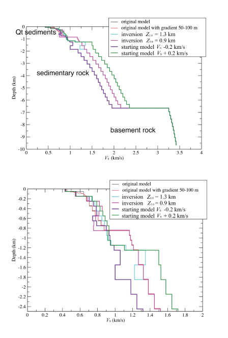
Shear-wave velocity (VS) profiles that fit observed group velocities. Top, VS profiles considered in this study. Bottom, Expanded view of profiles for depths less than 2 kilometers (km). Original velocity model is from the Stephenson and others (2017) three-dimensional model (SAO17) at location MP in figure 1, with VS in top 100 meters (m) set to 450 meters per second (m/s). The group velocities calculated for the revised models are shown in figure 6. Z1.0, depth to 1.0 kilometers per second (km/s).
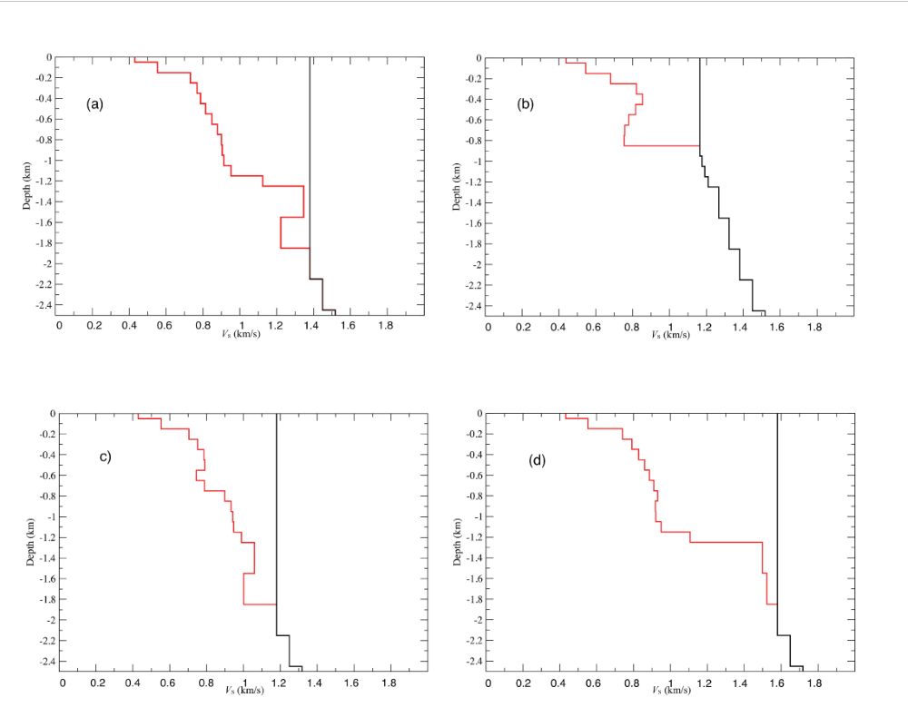
Plots of shear-wave velocity (VS) profiles involved in the inversions of group velocities. Black line is starting model for inversion; red line is model from inversion using observed group velocities. Predicted group velocities from inversions all fit observed group velocities. A, Inversion for layers shallower than 2.0 kilometers (km). B, Inversion for layers shallower than 0.9 km. C, Inversion for layers shallower than 2.0 km and lowering initial velocities by 0.2 kilometers per second (km/s) for depths greater than 2.0 km. D, Inversion for layers shallower than 2.0 km and raising initial velocities by 0.2 km/s for depths greater than 2.0 km.
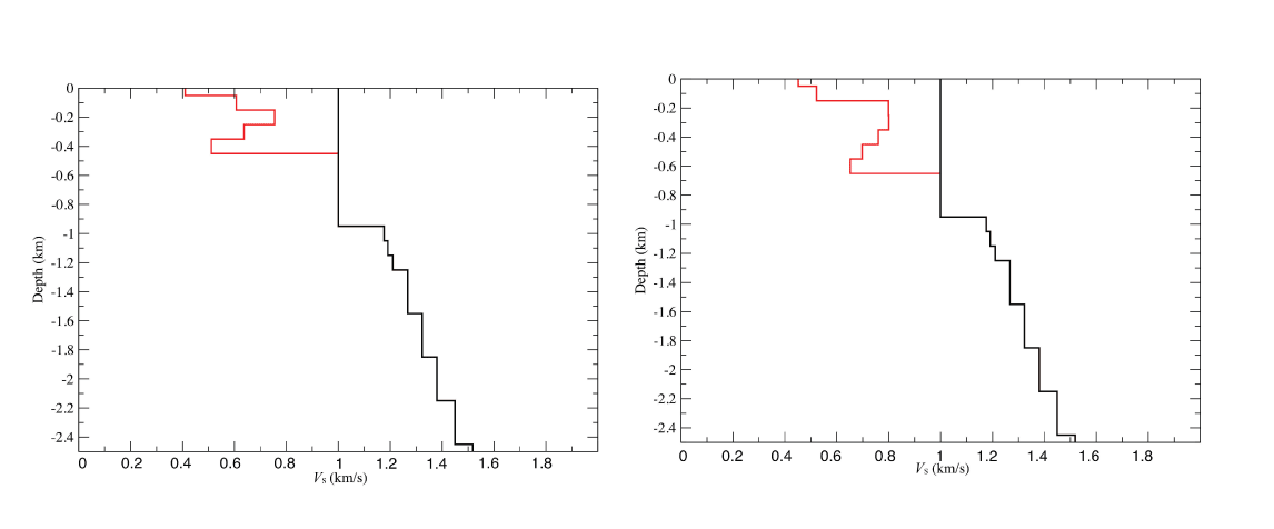
Shear-wave velocity (VS) profiles from the inversions for maximum depth-to-bedrock (Z1.0) values of 0.7 kilometers (km) (right) and 0.5 km (left). Black line is starting model for inversion; red line is model from inversion using observed group velocities. Predicted group velocities from inversions are shown in figure 6 and do not fit observed group velocities. km/s, kilometers per second.
Summary
This study demonstrated that the correlation of seismic noise with a short deployment time of 9 days is useful for evaluating the shear-wave velocity structure at depths to 2.4 km in the Seattle basin. We found several velocity profiles with depths to bedrock of 0.9 to 1.3 km that matched the observed group velocities. The results indicate that these noise data provide important information on the near-surface shear-wave velocity profiles and the depth to bedrock (Z1.0). These parameters are important in three-dimensional simulations, as well as empirical ground-motion models. Thus, relatively short deployments of instruments provide noise correlations that constrain the depth to bedrock in the Seattle basin, which is important for estimating ground motions from future earthquakes and, therefore, seismic hazard.
References Cited
Bensen, G.D., Ritzwoller, M.H., Barmin, M.P., Levshin, A.L., Lin, F., Moschetti, M.P., Shapiro, N.M., and Yang, Y., 2007, Processing seismic ambient noise data to obtain reliable broad-band surface wave dispersion measurements: Geophysical Journal International, v. 169, no. 3, p. 1239–1260, https://doi.org/10.1111/j.1365-246X.2007.03374.x.
Blakely, R.J., Wells, R.E., Weaver, C.S., and Johnson, S.Y., 2002, Location, structure, and seismicity of the Seattle fault zone, Washington—Evidence from aeromagnetic anomalies, geologic mapping, and seismic-reflection data: Geological Society of America Bulletin, v. 114, no. 2, p. 169–177, https://doi.org/10.1130/0016-7606(2002)114<0169:LSASOT>2.0.CO;2.
Brocher, T.M., 2005, Empirical relations between elastic wavespeeds and density in the Earth’s crust: Bulletin of the Seismological Society of America, v. 95, no. 6, p. 2081–2092, https://doi.org/10.1785/0120050077.
Calvert, A.J., Fisher, M.A., Johnson, S.Y., 2003, Along-strike variation in the shallow seismic velocity structure of the Seattle fault zone—Evidence for fault segmentation beneath Puget Sound: Journal of Geophysical Research, v. 108, no. B1, 14 p., https://doi.org/10.1029/2001JB001703.
Campbell, K.W., and Bozorgnia, Y., 2014, Ground motion model for the average horizontal components of PGA, PGV, and 5% damped linear acceleration response spectra: Earthquake Spectra, v. 30, p. 1087–1115, https://doi.org/10.1193/062913EQS175M.
Chiou, B.S.-J., and Youngs, R.R., 2014, Update of the Chiou and Youngs NGA model for the average horizontal component of peak ground motion and response spectra: Earthquake Spectra, v. 30, p. 1117-1153, https://doi.org/10.1193/072813EQS219M.
Delorey, A.A., and Vidale, J.E., 2011, Basin shear-wave velocity beneath Seattle, Washington, based on noise-correlated Rayleigh waves: Bulletin of the Seismological Society of America, v. 101, no. 5, p. 2162–2175, https://doi.org/10.1785/0120100260.
Frankel, A., Carver, D., and Williams, R., 2002, Nonlinear and linear site response and basin effects in Seattle for the M6.8 Nisqually, Washington, earthquake: Bulletin of the Seismological Society of America, v. 92, no. 6, p. 2090–2109, https://doi.org/10.1785/0120010254.
Frankel, A., and Stephenson, W., 2000, Three-dimensional simulations of ground motions in the Seattle region for earthquakes on the Seattle fault: Bulletin of the Seismological Society of America, v. 90, no. 5, p. 1251–1267, https://doi.org/10.1785/0119990159.
Frankel, A., Stephenson, W., and Carver, D., 2009, Sedimentary basin effects in Seattle, Washington—Ground-motion observations and 3D simulations: Bulletin of the Seismological Society of America, v. 99, no. 3, p. 1579–1611, https://doi.org/10.1785/0120080203.
Frankel, A.W., Stephenson, W., Carver, D., Williams, R., Odum, J., and Rhea, S., 2007, Seismic hazard maps for Seattle, Washington, incorporating 3D sedimentary basin effects, nonlinear site response, and rupture directivity: U.S. Geological Survey Open-File Report 2007–1175, 78 p., 3 pls., https://doi.org/10.3133/ofr20071175.
Frankel, A.D., Wirth, E.A., Marafi, N., Vidale, J.E., and Stephenson, W.J., 2018, Broadband synthetic seismograms for magnitude 9 earthquakes on the Cascadia megathrust based on 3D simulations and stochastic synthetics, Part 1—Methodology and overall results: Bulletin of the Seismological Society of America, v. 108, no. 5A, p. 2347–2369, https://doi.org/10.1785/0120180034.
Herrmann, R.B., 1973, Some aspects of band-pass filtering of surface waves: Bulletin of the Seismological Society of America, v. 63, no. 2, p. 663–671, https://doi.org/10.1785/BSSA0630020663.
Herrmann, R.B., 2013, Computer programs in seismology—an evolving tool for instruction and research: Seismological Research Letters, v. 84, p. 1081–1088, https://doi.org/10.1785/0220110096.
Johnson, S.Y., Dadisman, S.V., Childs, J.R., and Stanley, W.D., 1999, Active tectonics of the Seattle fault and central Puget Sound, Washington—Implications for earthquake hazards: Geological Society of America Bulletin, v. 111, no. 7, p. 1042–1053, https://doi.org/10.1130/0016-7606(1999)111<1042:ATOTSF>2.3.CO;2.
Lin, F.C., Moschetti, M.P., and Ritzwoller, M.H., 2008, Surface wave tomography of the western United States from ambient seismic noise—Rayleigh and Love wave phase velocity maps: Geophysical Journal International, v. 173, no. 1, p. 281–298, https://doi.org/10.1111/j.1365-246X.2008.03720.x.
Lobkis, O.I., and Weaver, R.L., 2001, On the emergence of the Green’s function in the correlation of a diffuse field: Journal of the Acoustical Society of America, v. 110, no. 6, p. 3011–3017, https://doi.org/10.1121/1.1417528.
Marafi, N.A., Eberhard, M.O., Berman, J.W., Wirth, E.A., and Frankel, A.D., 2019, Impact of simulated M9 Cascadia subduction zone motions on idealized systems: Earthquake Spectra, v. 35, no. 3, p. 1261–1287, https://doi.org/10.1193/052418EQS123M.
Odum, J.K., Stephenson, W.J., Goetz-Troost, K., Worley, D.M., Frankel, A.D., Williams, R.A., and Fryer, J., 2004, Shear- and compressional-wave velocity measurements from two 150-m-deep boreholes in Seattle, Washington, USA: U.S. Geological Survey Open-File Report 2004–1419, 36 p., https://doi.org/10.3133/ofr20041419.
Shapiro, N.M., and Campillo, M., 2004, Emergence of broadband Rayleigh waves from correlation of the ambient seismic noise: Geophysical Research Letters, v. 31, no. 7, L07614, 4 p., https://doi.org/10.1029/2004GL019491.
Snelson, C.M., Brocher, T.M., Miller, K.C., Pratt, T.L., and Trehu, A.M., 2007, Seismic amplification within the Seattle basin, Washington State—Insights from the SHIPS tomography experiments: Bulletin of the Seismological Society of America, v. 97, no. 5, p. 1432–1448, https://doi.org/10.1785/0120050204.
Stephenson, W.J., 2007, Velocity and density models incorporating the Cascadia subduction zone for 3D earthquake ground motion simulations: U.S. Geological Survey Open File Report 2007–1348, 24 p., https://pubs.usgs.gov/of/2007/1348/.
Stephenson, W., Asten, M., Odum, J., and Frankel, A., 2019, Shear-wave velocity in the Seattle basin to 2 km depth characterized with the krSPAC micotremor array method—Insights for urban basin-scale imaging: Seismological Research Letters, v. 90, no. 3, p. 1230–1242, https://doi.org/10.1785/0220180194.
Stephenson, W.J., Reitman, N.G., and Angster, S.J., 2017, P- and S-wave velocity models incorporating the Cascadia subduction zone for 3D earthquake ground motion simulations—Update for Open-File Report 2007–1348: U.S. Geological Survey Open-File Report 2017–1152, 17 p., https://doi.org/10.3133/ofr20171152.
Thompson, M., Wirth, E.A., Frankel, A.D., Hartog, J.R., and Vidale, J.E., 2020, Basin amplification effects in the Puget Lowland, Washington, from strong-motion recordings and 3D simulation: Bulletin of the Seismological Society of America, v. 110, no. 2, p. 534–555, https://doi.org/10.1785/0120190211.
Tsai, V.C., 2009, On establishing the accuracy of noise tomography travel-time measurements in a realistic medium: Geophysical Journal International, v. 178, no. 3, p. 1555–1564, https://doi.org/10.1111/j.1365-246X.2009.04239.x.
Williams, R.A., Stephenson, W.J., Frankel, A.D., and Odum, J.K., 1999, Surface seismic measurements of near surface P- and S-wave seismic velocities at earthquake recording stations, Seattle, Washington: Earthquake Spectra, v. 15, no. 3, p. 565–584, https://doi.org/10.1193/1.1586059.
Wirth, E.A., Frankel, A.D., Marafi, N., Vidale, J.E., and Stephenson, W.J., 2018, Broadband synthetic seismograms for magnitude 9 earthquakes on the Cascadia megathrust based on 3D simulations and stochastic synthetics, Part 2—Rupture parameters and variability: Bulletin of the Seismological Society of America, v. 108, no. 5A, p. 2370–2388, https://doi.org/10.1785/0120180029.
Wirth, E.A., Vidale, J.E., Frankel, A.D., Pratt, T.L., Marafi, N.A., Thompson, M., and Stephenson, W.R., 2019, Source-dependent amplification of earthquake ground motions in sedimentary basins: Geophysical Research Letters, v. 46, no. 12, p. 6443–6450, https://doi.org/10.1029/2019GL082474.
Wong, I., Stokoe, K.H., Cox, B.R., Lin, Y.-C., and Menq, F.-Y., 2011, Shear-wave velocity profiling of strong-motion sites that recorded the 2001 Nisqually, Washington, earthquake: Earthquake Spectra, v. 27, p. 183–212, https://doi.org/10.1193/1.3534936.
Abbreviations
GMM
ground-motion models
IRIS
Incorporated Research Institutions for Seismology
SAO17
Stephenson and others (2017) 3D velocity model
SPAC
spatially averaged coherency
USGS
U.S. Geological Survey
Suggested Citation
Frankel, A., and Bodin, P., 2022, Using seismic noise correlation to determine the shallow velocity structure of the Seattle basin, Washington: U.S. Geological Survey Open-File Report 2022–1108, 13 p., https://doi.org/10.3133/ofr20221108.
ISSN: 2331-1258 (online)
Study Area
| Publication type | Report |
|---|---|
| Publication Subtype | USGS Numbered Series |
| Title | Using seismic noise correlation to determine the shallow velocity structure of the Seattle basin, Washington |
| Series title | Open-File Report |
| Series number | 2022-1108 |
| DOI | 10.3133/ofr20221108 |
| Year Published | 2022 |
| Language | English |
| Publisher | U.S. Geological Survey |
| Publisher location | Reston, VA |
| Contributing office(s) | Earthquake Science Center |
| Description | vi, 12 p. |
| Country | United States |
| State | Washington |
| City | Seattle |
| Other Geospatial | Seattle Basin |
| Online Only (Y/N) | Y |
| Google Analytic Metrics | Metrics page |