

Estimating Northern Spotted Owl (Strix occidentalis caurina) Pair Detection Probabilities Based on Call-Back Surveys Associated with Long-Term Mark-Recapture Studies, 1993–2018
Links
- Document: Report (6.4 MB pdf) , HTML , XML
- Download citation as: RIS | Dublin Core
Acknowledgments
We thank the many field assistants who worked on the study areas over the years, as they were integral to the success of this effort. Federally funded study areas (Cle Elum, Olympia, Coast Ranges, HJ Andrews, Tyee, South Cascades, and Northwest California) collected data according to protocols approved by Oregon State University and Colorado State University’s Institutional Animal Care and Use Committees. All relevant State and Federal permits were acquired and maintained for all study areas included in this meta-analysis.
Abstract
The northern spotted owl (Strix occidentalis caurina; hereinafter NSO) was listed as “threatened” under the Endangered Species Act in 1990 and population declines have continued since that listing. Given the species’ protected status, any proposed activities on Federal lands that might impact NSO require consultation with U.S. Fish and Wildlife Service and part of that consultation often includes surveys to determine presence and occupancy status of the species in the proposed activity area. The objective of this report is to present study-area specific estimates of the probability of detection for NSO pairs from twelve 2-week seasonal survey periods using data from a recent range-wide meta-analysis. These estimates were a by-product of pair occupancy modeling but might provide insight into potential changes in the effect of the invasive barred owl on NSO detection rates. We used two-species multi-season occupancy models to estimate the probability of detection for NSOs on each of 11 study areas for each 2-week survey period and relative to the range-wide effect of barred owl presence or absence. Detection probabilities within the season generally increased from the earliest surveys in March through mid-season, decreasing again in the late season on five study areas. For three other study areas, detection rates were highest during the earliest survey periods in late March or early April. Estimates of cumulative seasonal detection of NSO (across a maximum of six within-season surveys) were less than 0.90 when barred owls (BO) were present on all but one study area, regardless of when surveys were conducted within a season. However, despite low detection rates, the probability that a territory was occupied when an NSO pair was not detected over six within-season surveys was also very low. When BO are not present on a territory, a six-survey protocol had a high probability of detecting an NSO pair at least once during the season on all study areas, except for the very lowest per-survey estimates. Conducting most surveys earlier in the season, when the probability of detecting pairs is highest (through May on most areas) could improve seasonal detection rates. However, alternative methods of population monitoring—such as the use of passive acoustic recorders—may be needed to continue monitoring NSO for research and management.
Introduction
The northern spotted owl (Strix occidentalis caurina; hereinafter NSO) was listed as “threatened” under the Endangered Species Act in 1990 (U.S. Fish and Wildlife Service, 1990). Because of continued population declines, the U.S. Fish and Wildlife Service (hereinafter USFWS) recently determined that uplisting NSO to “endangered” status was “warranted but precluded” by other listing priorities (U.S. Fish and Wildlife Service, 2020). Given the species’ protected status, any proposed activities on Federal lands that might impact NSO require consultation with USFWS, and part of that consultation often includes surveys to determine presence and occupancy status of this threatened species in the area of the proposed activity (U.S. Fish and Wildlife Service, 1992, 2012).
Detection of NSOs in forest stands incorporates two processes: (1) the probability that the territory is occupied (in other words, one or more NSO are present on the territory) and (2) the probability that if an NSO is present on the territory, it is detected. Thus, survey protocols and analyses that allow these two probabilities to be estimated separately provide the best estimates of territory occupancy and are important for documenting when planned management activities will negatively impact resident NSOs through habitat modifications or disruption to essential breeding activities. The primary method of surveying for NSOs in long-term demography studies includes as much as six call-back surveys conducted at fixed points along a route at night, or during walk-ins to previously occupied territory centers during the day (Franklin and others, 1996; Yackulic and others, 2012). As has been documented for some time, the invasive barred owl (Strix varia; hereinafter BO) suppresses NSO response rates to traditional call-back surveys (Olson and others, 2005; Crozier and others, 2006; Duchac and others, 2020). Barred owl presence on a territory also negatively impacts occupancy dynamics of NSO in the landscape (for example, Olson and others, 2005; Kroll and others, 2010; Dugger and others, 2011, 2016; Franklin and others, 2021). Therefore, NSO surveys that account for the probability of detection and BO presence provide the most robust estimates of NSO site occupancy.
Previously published estimates of NSO detection rates were based on per-visit detections (Olson and others, 2005; Kroll and others, 2010; Dugger and others, 2011), rather than equal-length survey periods that might include multiple territory visits (Yackulic and others, 2014; Dugger and others, 2016; Franklin and others, 2021). Early estimates also included detections of any owl—single or pair—and these per-visit detection rates were generally higher than detections of pairs only (Olson and others, 2005; Kroll and others, 2010). However, an owl pair is the ecological unit required to maintain viable populations so pair occupancy is vitally important to understanding population status and trends (Dugger and others, 2011). Recent efforts to understand occupancy dynamics of NSO have focused on detections of NSO pairs only (Yackulic and others, 2012, 2014, 2019; Dugger and others, 2011, 2016; Franklin and others, 2021). In these analyses, the estimation and modeling of NSO pair occupancy dynamics (for example, colonization, local extinction, annual occupancy) were the primary objective, so although the probability of detection was also always modeled, it was often not reported (for example, Dugger and others, 2016; Franklin and others, 2021).
The objective of this report is to present study-area specific estimates of the probability of detection for NSO pairs from twelve 2-week seasonal survey periods (“survey-specific”) using data from a recent meta-analysis of 11 NSO demographic study areas across the species range (Franklin and others, 2021). The NSO meta-analysis was not focused on estimating the probability of detecting NSO pairs, but such estimates were generated as a by-product of the pair occupancy modeling and might provide insight into potential changes into the continued effects of BOs on NSO detection rates. Since these estimates were not provided in Franklin and others (2021), they are presented in this report.
Study Areas
Populations of NSO that occurred on Federal and non-Federal lands within the range of the species were the basis of this analysis. To address our objectives, we used detection/non-detection survey data from historically monitored territories on 11 NSO demography studies included in the most recent meta-analysis evaluating population status and trends (table 1; fig. 1; Franklin and others, 2021). This analysis included three study areas in Washington (Cle Elum [CLE], Rainier [RAI], Olympic Peninsula [OLY]), five study areas in Oregon (Coast Ranges [COA], HJ Andrews [HJA], Tyee [TYE], Klamath [KLA], and South Cascades [CAS]), and three study areas in Northern California (Northwest California [NWC], Hoopa [HUP], Green Diamond Resources [GDR]; fig. 1). These study areas primarily represent lands under Federal administration, but some private, Tribal, and mixed ownership lands are also included (table 1). Detailed descriptions of each study area are available in Anthony and others (2006).
Table 1.
General characteristics of 11 study areas used to estimate probability of detection of northern spotted owl (Strix occidentalis caurina) pairs in Washington, Oregon and California, 1993–2018.[WA Douglas-fir refers to Pseudotsuga menziesii. Abbreviations: NW, Northwest; WA, Washington; OR, Oregon; CA, California; OR-CA, Oregon–California; km2, square kilometers]
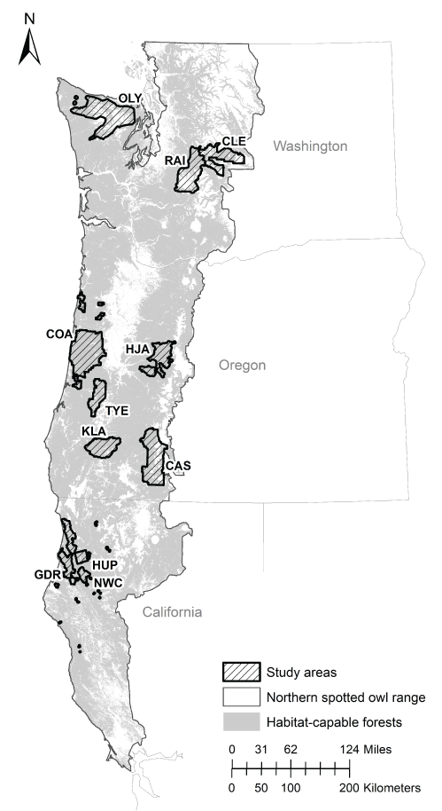
Locations of 11 study areas used to estimate per survey estimates of the probability of detection for northern spotted owl (Strix occidentalis caurina) pairs, Washington, Oregon, and California, 1993‒2018. Figure is taken from Dugger and others (2016).
Methods
Survey Data
Detection/non-detection data were collected annually for both NSO and BO across 26 years (1993–2018) on 9 study areas, 21 years (1993–2013) for HUP, and 16 years (1993–2008) for GDR. The total number of surveyed territories included in this analysis declined on two study areas (CLE, COA) in the last 4 years because we excluded territories involved in a concurrent BO removal study (for example, Wiens and others, 2021). Vocal lure (in other words, “callback”) surveys and daytime walk-in visits to previously used territory centers or nest trees were used to systematically search each study area for territorial NSOs (Franklin and others, 1996). The minimum number of visits per season ranged from three to six depending on the study area (Franklin and others, 1996). A detailed description of survey protocols associated with the NSO effectiveness monitoring program is available in appendix A of Lint and others (1999). Incidental detections (auditory and visual) of BOs were recorded as well as NSO detections. We grouped the results of territory visits into twelve 2-week survey periods (starting on March 1 and ending on August 31 of each year) that included detections of one or more BO and the distinction between single NSO and NSO pair detections during each survey period. Most study areas began surveys in early or late March of each year (period 1 or 2), but NWC began surveys in April (survey period 3) of each year. An NSO pair detection was defined as the detection of both the male and female NSO at some point during the 2-week survey period, the detection of a male NSO with a nest, or the detection of a single NSO of either sex with fledged young. We then summarized detection data within 2-week survey periods into encounter histories for any BO (singles or pairs) and NSO pairs only. Thus, to focus on detections of NSO pairs, detections of NSO singles were replaced with “0” (representing no detection of a pair) and “1” for pairs during a survey period, resulting in encounter histories that included four types of detections:
-
No owls were detected.
-
BOs only were detected.
-
NSO pairs only were detected.
-
Both BOs and an NSO pair were detected.
We used “dots” to denote missing data (in other words, no survey conducted within the 2-week survey period).
Analyses
Estimates of the probability of detection for NSOs were generated from two-species multi-season occupancy models (MacKenzie and others, 2018) using a hybrid of the approaches of Richmond and others (2010) and Yackulic and others (2014). For parameters modeled using the approach of Richmond and others (2010), we considered BOs the dominant species (coded as “A”) because of their prevalence and competitive advantage, and NSOs were the subordinate species (coded as “B”). The ecological process parameters were modeled as in Richmond and others (2010) and included initial occupancy (), colonization (γi), and local extinction (εi) for each species. These parameters are year-specific (subscript denotes primary sampling period “year”) and were modeled for BO as independent of NSO presence. For NSO, these parameters were modeled as conditional on whether BO were present or not. The probabilities of detection were survey-specific () within years () for each species () and were conditional on the presence (or not) of the other species as in Yackulic and others (2014), with estimates of the probability of detecting NSO pairs the focus of this report. We generated model parameter estimates as part of a meta-analysis effort that was focused on NSO demographics and included data from all 11 study areas (Franklin and others, 2021). We used program R-PRESENCE (https://www.mbr-pwrc.usgs.gov/software/presence.html) to build models and generate parameter estimates and model selection results. Detection probability () was estimated for each survey (secondary samples within seasons) within primary sampling periods (years) based on the model structure used in the meta-analysis (excluding the trap response; Franklin and others, 2021). We identified our best model for NSO pair detection rates using an information theoretics approach and AICc (Akaike’s Information Criteria corrected for small sample size) model selection results, with the model containing the lowest AICc generally considered to have the most support (Burnham and Anderson, 2002). The best probability of NSO pair detection model from our analysis included a study-area specific covariate, plus a study area-specific quadratic function reflecting within-season variation, and the additive effect of the presence of BOs that was shared across all study areas. No between season variation (denoted by the “.”) was included in the best model, only within-season variation (). We used the following equation to estimate the probability of detection of NSO pairs when BO were present:
We used the following equation to estimate the probability of detection of NSO pairs when BO were absent:
The survey period () was standardized [] and we used the resulting estimates of model coefficients (table 2) and the associated variance-covariance matrix to calculate survey-specific estimates that were constant across all years. We used the delta method (Cooch and White, 2021, Appendix B) and the embdbook package (v1.3.12; Bolker, 2008) in R 4.0.4 (R Core Team, 2021) to calculate standard errors (SE) and 95-percent confidence limits for these estimates. For more detail on the methodology and results relative to other model parameters, see Franklin and others (2021).
Table 2.
Model coefficients and standard errors from the model structure used to estimate survey-specific probability of detection for northern spotted owl (Strix occidentalis caurina) pairs on 11 study areas in Washington, Oregon, and California, 1993–2018.[The model included individual study area effects and the quadratic structure of survey occasion () for each study area, with the effect of barred owl (Strix varia) presence consistent across all season-specific surveys and study areas. There were twelve 2-week survey occasions (), and they were standardized [] before inclusion in the model. Abbreviations: OLY, Olympic; CLE, Cle Elum; RAI, Rainier; COA, Coast Ranges; HJA, HJ Andrews; TYE, Tyee; KLA, Klamath; CAS, South Cascades; HUP, Hoopa; GDR, Green Diamond; NWC, Northwest California; SE, standard error; , model coefficients]
We also used estimates to calculate a cumulative seasonal detection rate (), or the probability of detecting a NSO pair one time or more over the course of the season based on six surveys within a year (in other words, the highest minimum number of visits conducted per year on some study areas). We estimated under a robust design framework for each study area as follows:
We used four different combinations of estimates to calculate , including:
-
the single highest;
-
the single lowest;
-
the sixth highest (corresponding to the “peak” of the quadratic function); and
-
estimates from surveys 2, 4, 6, 8, 10, and 12, to reflect consistent survey effort over the 6-month NSO breeding season, for territories where BOs was present and territories where they were absent.
We also estimated the probability that NSO pairs were present even though they were never detected on any of six surveys conducted at a site within a season, for territories where BOs were present and territories where BOs were absent using Bayes’ Theorem (MacKenzie and others, 2018) as follows:
We calculated closed conditional probability of occupancy () based on six surveys per season () for territories with BOs present and territories with BOs absent. We used estimates of the probability of NSO pair territory occupancy in 2018 for each study area () and (1) the single highest and (2) six survey-specific detection probabilities () from surveys evenly spread across the season (in other words, surveys 2, 4, 6, 8, 10, 12) when BOs were present and when BOs were absent.
Results
Detection probabilities for within-season surveys for NSO pairs generally indicated a quadratic pattern, increasing from the earliest surveys in March through mid-season (May–June), decreasing again late in the season for five study areas (CLE, OLY, HJA, KLA, CAS; table 3; fig. 2). The pattern for COA and TYE was quadratic but the highest detection rates occurred earlier in the season, in late March or early April, and then decreased through the rest of the season (table 3; fig. 2). For the three California study areas (NWC, HUP, GDR) and one study area in Washington (RAI), the highest per-survey pair detection rates occurred during the earliest surveys in March and April and then decreased through the season to lows in August (fig. 2B, I–K). The additive effect of BO was negative for all study areas, with substantial reductions in per-survey NSO pair detection rates on all areas when BOs were present (table 3; fig. 2).
Table 3.
Estimates with standard errors and 95-percent confidence limits of the probability of detecting a northern spotted owl (Strix occidentalis caurina) pair on a territory if it is present when one or more barred owls (BO) are present, and when no barred owls (Strix varia) are present for twelve 2-week periods surveyed each year from March 1 to August 31 for Cle Elum, Rainier, Olympic, Coast Ranges, HJ Andrews, Tyee, Klamath, South Cascades, Northwest California, Hoopa, and Green Diamond Resources study areas, in Washington, Oregon, and California, 1993–2018.[Detection rates presented are from the best model, which does not include variation between years, only variation between surveys within years. The highest per-survey detection rates within a season are shown in bold type. Abbreviations: , estimates; SE, standard errors; 95% CI, 95-pecent confidence limits; --, no data]
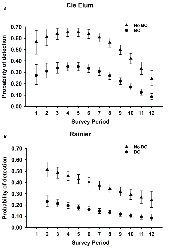
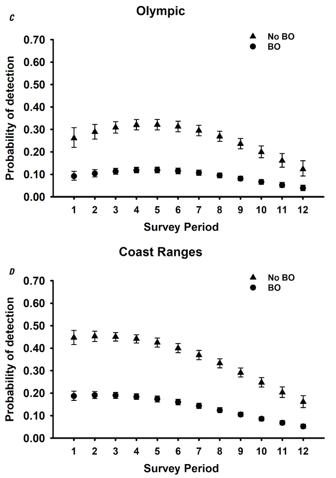
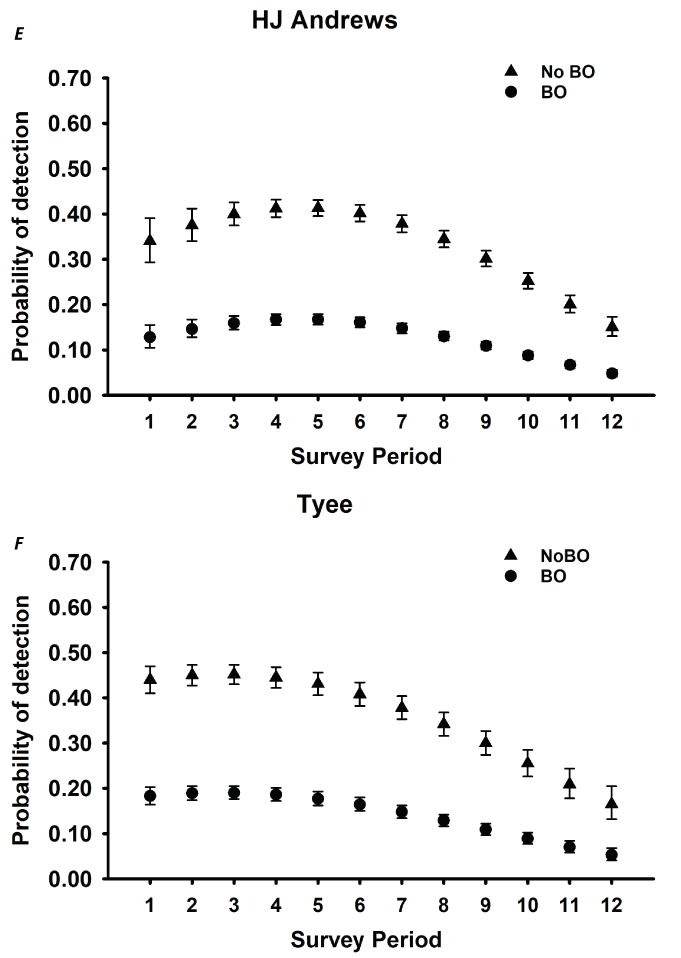
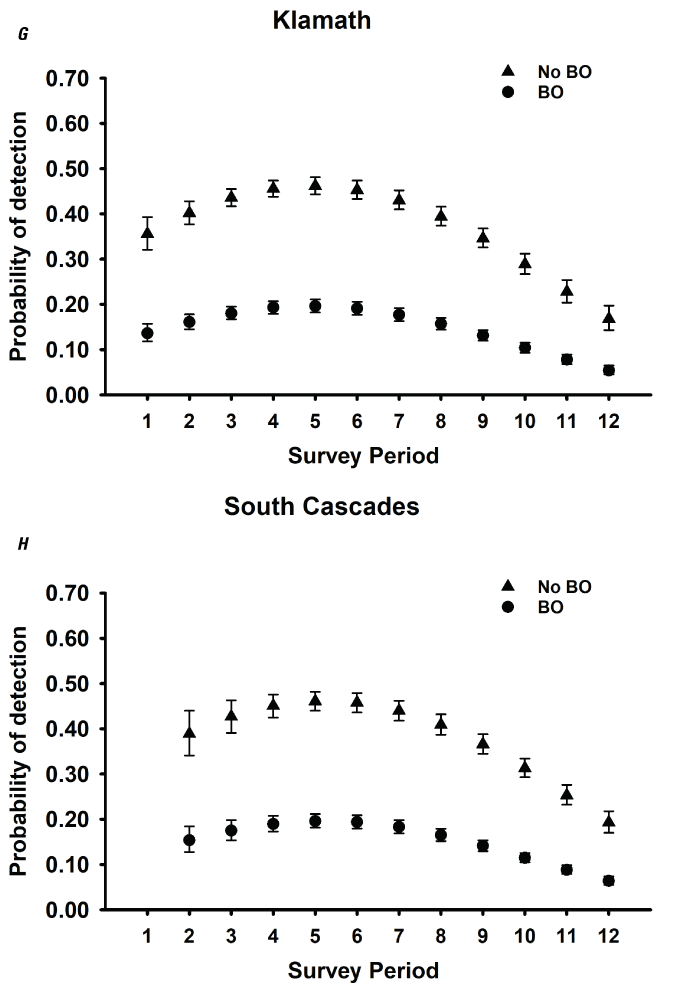
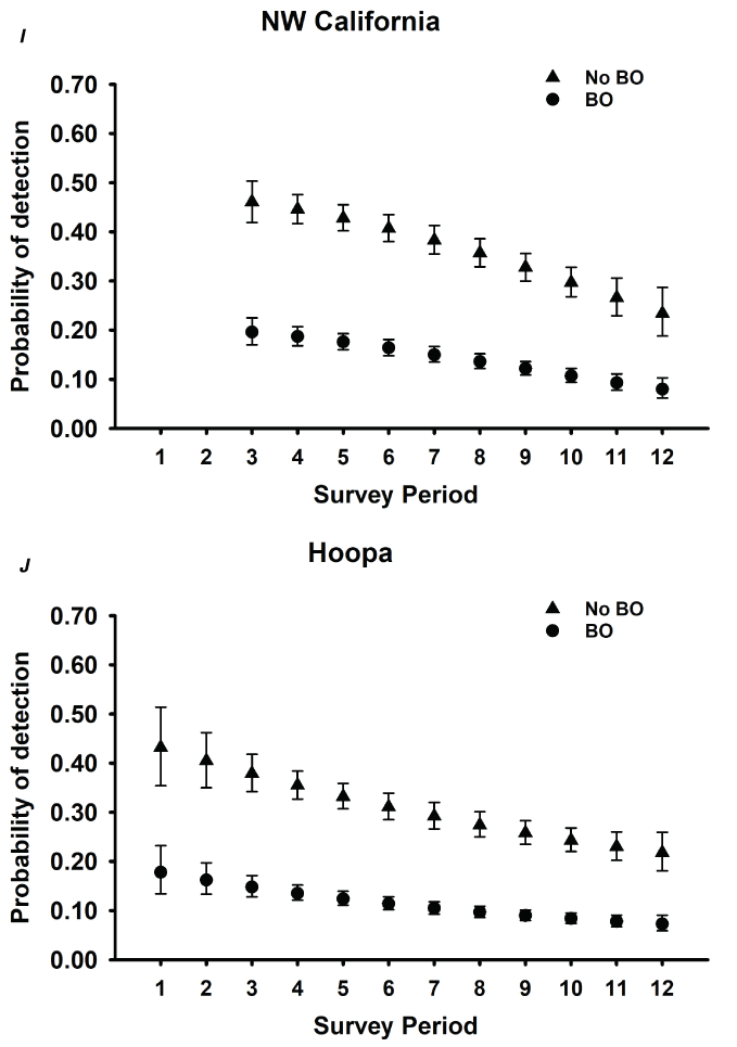

Estimates of detection probabilities with 95-percent confidence limits for northern spotted owl (Strix occidentalis caurina) pairs when barred owls (Strix varia; BO) are detected and when they are not across all twelve 2-week survey periods (March 1–August 31) conducted within seasons for Cle Elum (A), Rainier (B), Olympic (C), Coast Ranges (D), HJ Andrews (E), Tyee (F), Klamath (G), South Cascades (H), Northwest California (I), Hoopa (J), and Green Diamond Resources (K) study areas, Washington, Oregon, and California, 1993–2018. Surveys during period 1 in Rainier and South Cascades, and periods 1 and 2 in Northwest California were not conducted in any year, so estimates were excluded for those periods.
Estimates of cumulative seasonal detection of NSO pairs () from a maximum of six surveys were highest when based on either the single highest estimate or the six highest estimates. However, only CLE achieved greater than (>) 0.90 and represented the highest estimates of per-survey probability of detection when BOs were present (table 4). For most study areas the estimates of based on the six highest estimates varied from 0.60 to 0.75, but a low of 0.51 was observed on OLY and a high of 0.91 on CLE when BOs were present (table 4). In contrast, estimates of based on six surveys were >0.90 when BOs were not present on a territory for all configurations except for the lowest estimates (table 5), or when surveys 2,4,6,8,10, and 12 were used on OLY and HUP (table 5).
Table 4.
Cumulative seasonal detection () or the probability of detecting a northern spotted owl (Strix occidentalis caurina) pair one or more times when six surveys are conducted each year on each study area (see table 1) when one or more barred owls (Strix varia) are also present.[Estimates of were based on the (1) single highest, (2) single lowest, (3) six highest, and (4) estimates from survey periods 2, 4, 6, 8, 10, and 12 obtained from the best model, which does not include variation between years, but only variation between surveys within years.]
Table 5.
Cumulative seasonal detection () or the probability of detecting a northern spotted owl (Strix occidentalis caurina) pair one or more times when six surveys are conducted each year for each study area (see table 1) when no barred owls (Strix varia) are present. for each study area (see table 1).[Estimates of were based on the (1) single highest, (2) single lowest, (3) 6 highest, and (4) estimates from survey periods 2, 4, 6, 8, 10, and 12 obtained from the best model, which does not include variation between years, but only variation between surveys, within years.]
Despite low detection rates when BOs were present on a territory, conditional estimates of occupancy for territories where NSO pairs were never detected generally were also very low, particularly for the lowest per-survey pair detection rates and unconditional probability of occupancy for NSO pairs from 2018 when BOs were present (table 6). The probability that a territory was occupied when an NSO was not detected over six surveys was highest for study areas with the highest NSO pair occupancy rates and the lowest per-survey pair detection rates within seasons for both territories with and without BOs (table 6).
Table 6.
Estimates of the probability that a northern spotted owl pair (Strix occidentalis; NSO) is present, but not detected during a season when six surveys are conducted (in other words, closed conditional occupancy; ), based on Bayes’ Theorem following MacKenzie and others (2018) on 11 study areas in Washington, Oregon, and California.[Closed conditional occupancy was calculated using estimates of the probability of occupancy for NSO pairs during 2018 () and cumulative seasonal estimates of the probability of detection () based on the a) single highest and b) and survey-specific detection rates () for surveys 2, 4, 6, 8, 10, 12 on each study area when barred owls (Strix varia; BO) were present (see table 1) and when BOs were not present (table 2) from 2-species. occupancy models detailed in Franklin and others (2021).]
Discussion
For various ecological and analytical reasons, recent occupancy analyses for NSOs have focused on detections of NSO pairs (Dugger and others, 2011, 2016; Yackulic and others, 2012; 2014; Franklin and others, 2021) rather than detection of any owl, single or pair. From the perspective of understanding population status and trends, territorial occupancy of NSO pairs is the relevant ecological metric. We observed variation in the survey-specific probability of detecting a pair over the course of the breeding season with five study areas having the highest per-survey detection rates in May, consistent with earlier findings by Yackulic and others (2014) on TYE. However, we observed the highest per-survey detection rates earlier in the season (March or April) for all California study areas, and on RAI in Washington, and COA and TYE in Oregon, suggesting that the timing of the most efficient survey effort might be different depending on the study area.
Our estimates of the probability of detection of NSO pairs based on 2-week time periods during the season (per-survey estimates) were 29–59 percent lower than previous estimates for any owl (single or pair) on the same study areas (OLY, CLE, COA, HJA, TYE, CAS; Dugger and others, 2009; table 7). However, our findings were similar to mean per-visit detection rates of owl pairs in Oregon and California across territories with and without BOs (Olson and others, 2005, Kroll and others, 2010). Estimates of the probability of detection of NSO pairs from these earlier studies varied by season but were often less than (<) 0.40 (0.22–0.67; fig. 3 in Olson and others, 2005; 0.27–0.67; fig. 3 in Kroll and others, 2010). On the CAS study area, previous estimates of per-visit detection rates for NSO pairs when BOs were present were often <0.20, as compared to rates >0.50 when BOs were absent (Dugger and others, 2011), consistent with current findings for CAS at least when BOs were present in territories (table 3). Thus, detection rates of pairs in response to BO presence may not have changed substantially in the last 10 years, at least in some areas.
Table 7.
Estimates, standard errors, and 95-percent confidence limits of the highest survey-specific probability of detection for northern spotted owl (Strix occidentalis caurina) pairs when barred owls (Strix varia) are present for each study area (mean across all years 1993–2018; table 1) in comparison to mean, within season visit-specific estimates for singles and pairs from previous analyses (see table 1; Dugger and others, 2009).[Abbreviations: , estimates (first number on left side of column), standard errors (first number inside parentheses), and 95-percent confidence limits (number range within parentheses) of the highest survey-specific probability of detection for northern spotted owl pairs; N/A, study areas not included in Dugger and others (2009).]
| Study Area | This study | Dugger and others (2009) |
|---|---|---|
| Washington | ||
| Cle Elum | 0.35 (0.09; 0.31–0.39) | 0.49 (0.04; 0.42–0.57) |
| Rainier | 0.23 (0.08; 0.19–0.28) | N/A |
| Olympic | 0.12 (0.02; 0.11–0.13) | 0.36 (0.02; 0.33–0.40) |
| Oregon | ||
| Coast Ranges | 0.19 (0.02; 0.18–0.21) | 0.46 (0.02; 0.42–0.50) |
| HJ Andrews | 0.17 (0.02; 0.16–0.18) | 0.40 (0.04; 0.33–0.48) |
| Tyee | 0.19 (0.02; 0.18–0.21) | 0.37 (0.04; 0.30–0.45) |
| Klamath | 0.20 (0.05; 0.18–0.21) | N/A |
| South Cascades | 0.20 (0.02; 0.18–0.21) | 0.29 (0.02; 0.42–0.50) |
| California | ||
| Northwest California | 0.20 (0.04; 0.17–0.23) | N/A |
| Hoopa | 0.18 (0.07; 0.13–0.23) | N/A |
| Green Diamond Resources | 0.21 (0.04; 0.19–0.24) | N/A |
Estimates of detection rates for NSO pairs across 2-week survey periods are not necessarily equivalent to per-visit detection rates reported in previous studies as per-visit detections reflected a single complete territory survey (for example, Olson and others, 2005; Dugger and others, 2011), whereas the 2-week time periods used in our analysis could include the results of less than one complete territory survey. Additionally, detection rates for pairs can be substantially lower than estimates for any owl (both singles and pairs; Olson and others, 2005; Kroll and others, 2010). As a result, cumulative seasonal detection rates for NSO pairs () from this study when BOs were present were less than 0.95 on all study areas except CLE under a six-survey protocol (table 8). Increasing the number of surveys within a season could increase the probability of detecting an NSO pair at least once during the season, but the number of surveys required to meet a target of >0.95 or even >0.90 would range from 8 to >12 depending on the study area (table 8). Additionally, the extra calling by field crews could also create more negative consequences for breeding NSO because of the increased territory that defense callbacks elicit, or the potential for increased interactions with resident BO that might occur when NSO respond to callbacks. Alternatively, conducting most surveys earlier in the season, when the probability of detecting pairs is highest (through May on most areas) could improve seasonal detection rates. When BO are not present on a territory, a six-survey protocol had a high probability of detecting an NSO pair at least once during the season on all study areas, except for the very lowest estimates (table 8).
Table 8.
Probability of detecting a northern spotted owl (Strix occidentalis caurina) pair on a territory at least one time during the season given it is present (), relative to the total number of surveys conducted each season (range 3–12), when one or more barred owl (Strix varia) was present, and when barred owls were not present for Cle Elum, Rainier, Olympic, Coast Ranges, HJ Andrews, Tyee, Klamath, South Cascades, Northwest California, Hoopa, and Green Diamond Resources study areas, Washington, Oregon, and California.[The single highest survey-specific detection rate () observed across all years for each study area (see table 3) was used to calculate . Abbreviation: BO, barred owl.]
In contrast to detection rates, occupancy dynamics have changed substantially since the mid-to late-2000s. Colonization rates have declined and local extinction rates have increased for NSO populations in all study areas coincident with the increasing presence of BO in the landscape (Franklin and others, 2021). These changes in occupancy dynamics have resulted in strong declines in territory occupancy (fig. 9 in Franklin and others, 2021) and increased rates of movement between territories (in other words, breeding dispersal) by NSOs (Jenkins and others, 2021). This result is consistent with overall declines in rates of population change, suggesting that NSO populations continue to decline range-wide (Franklin and others, 2021). Smaller NSO populations and declines in the probability of pair territory occupancy can impact the cumulative seasonal probability of detecting NSO pairs during surveys. Although a six-survey protocol has a high probability of detecting an NSO pair at least once during the season if BO are not present on the territory, by 2018, BO occupancy on NSO territories ranged from 0.49 to 0.97 (fig. 9 in Franklin and others, 2021). Thus, very few NSO territories included in this analysis were not impacted by BO. Consequently, NSO pair occupancy rates observed in 2018 by Franklin and others (2021) were low in many study areas (<0.25 on seven areas). For these study areas, the probability of never detecting NSO pairs within a season, given that they were present (in other words, closed conditional occupancy) when six surveys were conducted, was generally <0.10 for the highest per-survey detection rates observed when BOs were present. Thus, when occupancy rates are very low, the probability of missing an NSO pair if it was present using a six-survey protocol was low, even though per-survey detection rates were also very low. When BOs were not present, estimates on all study areas were generally high enough that there was a low probability of incorrectly assigning pair occupancy status to a territory under a six-survey protocol (in other words, closed conditional occupancy was <0.10 on most study areas; table 6).
Alternative methods of population monitoring—such as the use of passive acoustic monitoring where as little as 3 weeks of recording can document the presence/absence of NSO (singles or pairs) with 95-percent certainty (Wood and others, 2019; Duchac and others, 2020)—may be needed to continue monitoring NSO for research and management (Lesmeister and others, 2021). However, these estimates of the probability of detection are not directly comparable to our estimates of the probability of detecting NSO pairs. These studies have used random grid sampling that estimated the probability of use rather than occupancy of historical territories and estimated detection of any NSO (singles and pairs; Wood and others, 2019; Duchac and others, 2020). Advances in processing and interpretation of acoustic data are ongoing and distinguishing between the sexes (Dale and others, 2022), territory residence, and breeding status (in other words, transients, resident singles, and pairs) may be possible using calling frequency and timing. However, the delineation of NSO activity centers would likely require additional survey effort (walk-ins in addition to the use of passive acoustic monitoring) to provide the information currently used to protect NSO in forest stands proposed for harvest (Duchac and others, 2020). Alternatively, the trigger for stand protection could shift from identifying an occupied NSO activity center to identifying any stand with some specified level of “use” by NSO (Lesmeister and others, 2021).
Changes in NSO pair occupancy rates across the species range (for example, Franklin and others, 2021), and BO effects on NSO behavior including decreased detection rates, and longer, and more likely movement of breeding birds (Jenkins and others, 2019, 2021) has increased the difficulties of monitoring NSO. However, it is critical to NSO conservation and management to understand where on the landscape productive NSO pairs exist, particularly when proposed management activities may negatively impact those pairs. BO control strategies can be successful at halting or reversing declines in NSO populations (Diller and others, 2016; Wiens and others, 2021); however, these activities can only be successful if suitable habitat is available for NSO to recolonize after BO are controlled.
References Cited
Anthony, R.G., Forsman, E.D., Franklin, A.B., Anderson, D.R., Burnham, K.P., White, G.C., Schwarz, C.J., Nichols, J.D., Hines, J.E., Olson, G.S., Ackers, S.H., Andrews, L.S., Biswell, B.L., Carlson, P.C., Diller, L.V., Dugger, K.M., Fehring, K.E., Fleming, T.L., Gerhardt, R.P., Gremel, S.A., Gutiérrez, R.J., Happe, P.J., Herter, D.R., Higley, J.M., Horn, R.B., Irwin, L.L., Loschl, P.J., Reid, J.A., and Sovern, S.G., 2006, Status and trends in demography of northern spotted owls, 1985–2003: Wildlife Monographs, v. 163, p. 1–48.
Cooch, E., and White, G.C., eds., 2021, The delta method, app. B of Program MARKA gentle introduction (19th ed.): phpBB Group, 44 p., accessed December 9, 2021, at http://www.phidot.org/software/mark/docs/book/pdf/app_2.pdf.
Dugger, K.M., Forsman, E.D., Franklin, A.B., Davis, R.J., White, G.C., Schwarz, C.J., Burnham, K.P., Nichols, J.D., Hines, J.E., Yackulic, C.B., Doherty, P.F., Jr., Bailey, L., Clark, D.A., Ackers, S.H., Andrews, L.S., Augustine, B., Biswell, B.L., Blakesley, J., Carlson, P.C., Clement, M.J., Diller, L.V., Glenn, E.M., Green, A., Gremel, S.A., Herter, D.R., Higley, J.M., Hobson, J., Horn, R.B., Huyvaert, K.P., McCafferty, C., McDonald, T., McDonnell, K., Olson, G.S., Reid, J.A., Rockweit, J., Ruiz, V., Saenz, J., and Sovern, S.G., 2016, The effects of habitat, climate, and barred owls on long-term demography of northern spotted owls: The Condor, v. 118, no. 1, p. 57–116.
Franklin, A.B., Dugger, K.M., Lesmeister, D.B., Davis, R.J., Wiens, J.D., White, G.C., Nichols, J.D., Hines, J.E., Yackulic, C.B., Schwarz, C.J., Ackers, S.H., Andrews, L.S., Bailey, L.L., Bown, R., Burgher, J., Burnham, K.P., Carlson, P.C., Chestnut, T., Conner, M.M., Dilione, K.E., Forsman, E.D., Glenn, E.M., Gremel, S.A., Hamm, K.A., Herter, D.R., Higley, J.M., Horn, R.B., Jenkins, J.M., Kendall, W.L., Lamphear, D.W., McCafferty, C., McDonald, T.L., Reid, J.A., Rockweit, J.T., Simon, D.C., Sovern, S.G., Swingle, J.K., and Wise, H., 2021, Range-wide declines of northern spotted owls populations in the Pacific Northwest—A meta-analysis: Biological Conservation, v. 259, p. 109168, accessed December 9, 2021, at https://doi.org/10.1016/j.biocon.2021.109168.
Jenkins, J.M.A., Lesmeister, D.B., Forsman, E.D., Dugger, K.M., Ackers, S.H., Andrews, L.S., Gremel, S.A., Hollen, B., McCafferty, C.E., Pruett, M.S., Reid, J.A., Sovern, S.G., and Wiens, J.D., 2021, Conspecific and congeneric interactions shape increasing rates of breeding dispersal of northern spotted owls: Ecological Applications, v. 31, no. 7, p. e02398.
Jenkins, J.M.A, Lesmeister, D.B., Forsman, E.D., Dugger, K.M., Ackers, S.H., Andrews, L.S., McCafferty, C.E., Pruett, M.S., Reid, J.A., Sovern, S.G., Horn, R.B., Gremel, S.A., Wiens, J.D., and Yang, Z., 2019, Social status, forest disturbance, and barred owls shape long-term trends in breeding dispersal distance of northern spotted owls: Condor v. 121, no. 4, p. 45–62.
Lesmeister, D.B., Appel, C.L., Davis, R.J., Yackulic, C.B., and Ruff, Z.J., 2021, Simulating the effort necessary to detect changes in northern spotted owl (Strix occidentalis caurina) populations using passive acoustic monitoring, PNW-RP-618: Portland, Oregon, U.S. Forest Service, Pacific Northwest Research Station, 55 p.
Olson, G.S., Anthony, R.G., Forsman, E.D., Ackers, S.H., Loschl, P.J., Reid, J.A., Dugger, K.M., Glenn, E.M., and Ripple, W.J., 2005, Modeling of site occupancy dynamics for northern spotted owls, with emphasis on the effects of barred owls: The Journal of Wildlife Management, v. 69, no. 3, p. 918–932.
R Core Team, 2021, R: A language and environment for statistical computing: Vienna, Austria, R Foundation for Statistical Computing, accessed December 9, 2021, at https://www.R-project.org/.
Wiens, J.D., Dugger, K.M., Higley, M., Lesmeister, D.B., Franklin, A.B., Hamm, K., White, G.C., Dilione, K., Simon, D.C., Brown, R., Carlson, P., Yackulic, C., Nichols, J., Hines, J., Davis, R., Lamphear, D., McCafferty, C., McDonald, T., Sovern, S., and Sovern, S., 2021, Invader removal triggers competitive release in a threatened avian predator: Proceedings of the National Academy of Sciences of the United States of America, v. 118, no. 31, p. e2102859118, accessed December 9, 2021, at https://doi.org/10.1073/pnas.2102859118.
Yackulic, C.B., Bailey, L.L., Dugger, K.M., Davis, R.J., Franklin, A.B., Forsman, E.D., Ackers, S.H., Andrews, L.S., Diller, L.V., Gremel, S.A., Hamm, K.A., Herter, D.R., Higley, J.M., Horn, R.B., McCafferty, C., Reid, J.A., Rockweit, J.T., and Sovern, S.G., 2019, The past and future roles of competition and habitat in the range-wide occupancy dynamics of northern spotted owls: Ecological Applications, v. 29, no. 3, p. e01861.
Conversion Factors
Datum
Horizontal coordinate information is referenced to the North American Datum of 1983 (NAD 83_Albers).
Abbreviations
AICc
Akaike’s information criteria, corrected for small sample sizes
BO
barred owl
CAS
South Cascades
CI
confidence interval
CLE
Cle Elum
COA
Coast Ranges
GDR
Green Diamond Resources
HJA
HJ Andrews
HUP
Hoopa
KLA
Klamath
NSO
northern spotted owl
NWC
Northwest California
OLY
Olympic
RAI
Rainier
SE
standard error
TYE
Tyee
USFWS
U.S. Fish and Wildlife Service
For information about the research in this report, contact
Director, Forest and Rangeland Ecosystem Science Center
777 NW 9th Street
Suite 400
Corvallis, OR 97330
https://www.usgs.gov/centers/forest-and-rangeland-ecosystem-science-center
Manuscript approved on February 6, 2023.
Publishing support provided by the U.S. Geological Survey
Science Publishing Network, Tacoma Publishing Service Center
Suggested Citation
Dugger, K.M., Franklin, A.B., Lesmeister, D.B., Davis, R.J., Wiens, J.D., White, G.C., Nichols, J.D., Hines, J.E., Yackulic, C.B., Schwarz, C.J., Ackers, S.H., Andrews, L.S., Bailey, L.L., Bown, R., Burgher, J., Burnham, K.P., Carlson, P.C., Chestnut, T., Conner, M.M., Dilione, K.E., Forsman, E.D., Gremel, S.A., Hamm, K.A., Herter, D.R., Higley, J.M., Horn, R.B., Jenkins, J.M., Kendall, W.L., Lamphear, D.W., McCafferty, C., McDonald, T.L., Reid, J.A., Rockweit, J.T., Simon, D.C., Sovern, S.G., Swingle, J.K., and Wise, H., 2023, Estimating northern spotted owl (Strix occidentalis caurina) pair detection probabilities based on call-back surveys associated with long-term mark-recapture studies, 1993–2018: U.S. Geological Survey Open-File Report 2023–1012, 25 p., https://doi.org/10.3133/ofr20231012.
ISSN: 2331-1258 (online)
Study Area
| Publication type | Report |
|---|---|
| Publication Subtype | USGS Numbered Series |
| Title | Estimating northern spotted owl (Strix occidentalis caurina) pair detection probabilities based on call-back surveys associated with long-term mark-recapture studies, 1993–2018 |
| Series title | Open-File Report |
| Series number | 2023-1012 |
| DOI | 10.3133/ofr20231012 |
| Year Published | 2023 |
| Language | English |
| Publisher | U.S. Geological Survey |
| Publisher location | Reston, VA |
| Contributing office(s) | Coop Res Unit Seattle, Forest and Rangeland Ecosys Science Center, Patuxent Wildlife Research Center, Southwest Biological Science Center, Eastern Ecological Science Center |
| Description | vii, 25 p. |
| Country | United States |
| State | California, Oregon, Washington |
| Online Only (Y/N) | Y |
| Google Analytic Metrics | Metrics page |