

Light Attenuation and Erosion Characteristics of Fine Sediments in a Highly Turbid, Shallow, Great Basin Lake—Malheur Lake, Oregon, 2017–18
Links
- Document: Report (4.2 MB pdf) , HTML , XML
- Data Releases:
- USGS data release — Phytoplankton data for Malheur Lake, Oregon, 2018-20
- USGS data release — Photosynthetically active radiation measurements collected at Malheur Lake, Oregon, 2017-18
- Download citation as: RIS | Dublin Core
Acknowledgments
The authors thank the High Desert Partnership and U.S. Fish and Wildlife Service for their collaboration and partnership during this study. Data collection was facilitated by Joe Barnett, Alexa Martinez, Ed Sparks, Norman Clippinger, Ben Cate, Robert Esquivel, Shelly Pickett, and James Pearson, all presently or formerly with one of these two organizations. We appreciate David Schoelhammer (U.S. Geological Survey emeritus) for volunteering his time and expertise with the mobile erosion laboratory, and we thank Sara Eldridge and Liam Schenk (U.S. Geological Survey) for their efforts leading the project in various years.
Abstract
Malheur Lake is a large, shallow, turbid lake in southeastern Oregon that fluctuates widely in surface area in response to yearly precipitation and climatic cycles. High suspended-sediment concentrations (SSCs) likely are negatively affecting the survival of aquatic plants by reducing the intensity of solar radiation reaching the plants, thus inhibiting photosynthesis. This study was designed to determine the types of suspended material, the erodibility of the lakebed, the attenuation of photosynthetically active radiation (PAR) through the water column, and the effects of wind and precipitation on SSC.
Two sites in the lake were monitored for approximately 5 months during the summer growing season each year (2017–19). At these sites, turbidity, chlorophyll a fluorescence (a surrogate for concentration), and underwater PAR measurements were collected continuously, and discrete samples were collected every 2 weeks and analyzed for SSC, loss on ignition, and chlorophyll a concentration. Underwater PAR profile measurements were collected during site visits, and a nearby meteorological station recorded terrestrial PAR and wind speeds.
About 18 percent of suspended material in the water was organic and mostly detrital. Nearly 100 percent of all suspended material was fine material (less than 63 micrometers), and more than 90 percent of the surficial lakebed material was fine material. The high concentrations of fine material in the water column can be expected to strongly attenuate light.
SSC was significantly higher at both sites in 2018 compared to 2017 and 2019; the interannual differences were mostly due to the lower amount of precipitation in 2018, which resulted in shallower lake depths. Three years of SSC values multiplied by water depth ( showed a seasonal pattern: concentrations were often highest in early spring, lowest in summer, and intermediate in autumn.
Episodic wind events with speeds of 5–10 meters per second caused rapid increases in turbidity above background that lasted for a few days. However, a baseline (estimated to be 0.11 kilograms per square meter) was present between wind events and even under ice, suggesting a persistent suspension of very fine, highly erodible material. Terrestrial and underwater PAR measurements were used to develop a relation between PAR attenuation and turbidity that can be used in modeling restoration scenarios. Calculated bottom shear stress caused by wind-generated waves ranged from 0 to 0.4 pascals (Pa). Erosion experiments indicated variability in the bottom sediments from the two lake sites, but much of the lakebed is highly erodible at a threshold of 0.05 to 0.1 Pa.
Restoration actions may target the persistent turbidity (for example, the use of flocculation) or transient turbidity (for example, construction of wave-reduction barriers), with a goal of attaining approximately 36 micromoles photons per square meter per second of PAR at the lakebed to promote emergence of sago pondweed and other desirable plants. Currently, that threshold often is reached from 4 to 34 centimeters (cm) below the water surface in 1 meter water depth, depending on wind conditions, but halving persistent turbidity would increase the upper end of the range to 55 cm. Additional studies regarding the effects of (1) sediment drying on resuspension and (2) nutrient inputs and internal cycling on phytoplankton populations would help determine the most appropriate restoration strategies.
Introduction
Malheur Lake is a large and shallow terminal wetland-lake system in the semi-arid northwestern corner of the Great Basin of the continental United States, in southeastern Oregon (fig. 1). President Theodore Roosevelt established the Malheur National Wildlife Refuge in 1908 because the lake system was one of the largest freshwater marshes in the United States and served as an important stop and breeding ground along the Pacific Flyway for migratory birds (Cornely, 1982). The refuge is managed by the U.S. Fish and Wildlife Service. Despite degradation of habitat in recent years, the lake is still an important breeding and migration area for ducks and geese, breeding area for numerous shorebird species, and habitat for resident species (Duebbert, 1969; Cornely, 1982; U.S. Fish and Wildlife Service, 2012).
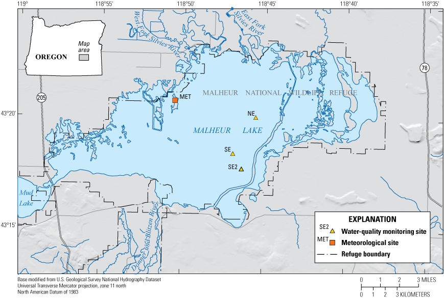
Malheur Lake and monitoring locations, southeastern Oregon. Water-quality monitoring sites NE (northeast) and SE (southeast) were monitored in 2017. Water-quality monitoring sites NE and SE2 (SE site moved to a different location) were monitored in 2018 and 2019.
A defining feature of Malheur Lake is its large range in area over multidecadal time scales, resulting from climatic cycles in annual precipitation and snowpack. In the past century (1920–2020), the surface area of the lake has varied over 2 orders of magnitude, from low values of about 500 hectares (ha) in 1992 to about 54,000 ha in 1986, as well as smaller maxima around 30,000 ha at earlier and later times in the 20th century (Pearson, 2020). The lake has two major freshwater inputs, the Silvies River and the Donner und Blitzen River. The Silvies River—the smaller of the two—flows into the lake from the north, and its headwaters are in the high elevations of the Blue Mountains in central Oregon. The Silvies River is connected to the lake only through surface flow during times of high snowmelt runoff; it is not connected through surface flow every year, depending on the snowpack (Hubbard, 1975). The Donner und Blitzen River flows into the lake from the south, and its headwaters are in the high elevations of the Steens Mountain area of southeastern Oregon. The Donner und Blitzen River is perennial, but the annual hydrograph follows a standard snowmelt-driven progression from the highest flows in the spring as snowpack melts to lowest flows, primarily groundwater-sourced base flow, in late summer and autumn.
As recently as the 1970s, Malheur Lake was a vast wetland, containing both emergent vegetation (dominated by hardstem bulrush [Schoenoplectus acutus]) and submergent vegetation (dominated by sago pondweed [Stuckenia pectinata]; Duebbert, 1969). However, the lake is currently (2021) a highly turbid environment, with a lack of aquatic vegetation of either type, characterized by high concentrations of nutrients and suspended sediment. The suspended-sediment concentrations (SSCs) in Malheur Lake, at times exceeding 1,000 milligrams per liter (mg/L) in this study, are much higher than the concentrations in other shallow, freshwater systems around the world that have been characterized as highly turbid (Dokulil, 1984; Lee and Rast, 1997; Chen and others, 2003; Jeppesen and others, 2003; Guang and others, 2006), where the highest values of suspended sediment rarely exceed 150 mg/L. The lake’s resident fish assemblage has been diminished and is now dominated by the non-native, benthivorous common carp (Cyprinus carpio). Modeling results suggest that the population of carp has progressed through boom-and-bust cycles over the decades, largely responding to, and lagging, the size of the lake; peak biomass has reached 10,000 kilograms per hectare multiple times (Pearson, 2020). Those high carp biomasses likely played an important role in eliminating aquatic vegetation from the system. Much of the restoration activity directed at the lake ecosystem has focused on elimination of carp (Pearson and others, 2019), but there has recently been recognition that the system has progressed down the path of high turbidity to a stable state such that even if carp could be eliminated, that alone will likely not be enough to bring the system back to a macrophyte-dominated stable state.
A paradigm in the study of shallow lakes is that they can exist in one of two alternate stable states—(1) a clear state, characterized by an abundance of aquatic macrophytes, diverse aquatic biota, and low water column nutrients and phytoplankton biomass, and (2) a turbid state, characterized by the opposite (Scheffer and others, 1993; Scheffer and others, 2001). A shift from a clear to a turbid state can be induced by several physical or ecological factors and interactions among the factors, including climatic drivers, nutrient fluxes, hydrologic variability, biotic invaders, and loss of native species. An important aspect of this paradigm is that these factors can also increase the system’s resistance to a shift between states because feedbacks reinforce the new system (Scheffer, 2004). Once an alternative turbid state is reached, therefore, the threshold for returning to the clear state may require nutrient or suspended-sediment concentration or invasive species biomass that is lower than it was before the switch in states. This study is part of an ongoing effort of managers and interest groups to identify the feedback mechanisms that maintain the turbid state at Malheur Lake and to determine the threshold that must be achieved through restoration activities to return the lake to its previous, clear state.
Purpose and Scope
The purpose of this study was to determine the effect of suspended particles in Malheur Lake on the depth of light penetration through the water column. Plants require light, specifically photosynthetically active radiation (PAR, visible light in the 400–700 nanometer [nm] wavelength range), to photosynthesize. Therefore, scattering and absorption of light from suspended particles directly affect plant survival. The objectives of the study were to evaluate the:
-
mass of particles in the water column (volumetric concentration and mass density),
-
type of particles in the water column (inorganic, organic, fine material, coarse material),
-
source of particles, whether from tributaries or limnetic (resuspension of bed material or autochthonous growth of organic material),
-
effect of wind speed and precipitation on concentration of suspended particles,
-
interannual and seasonal effects (such as water depth and ice cover) on the concentration of suspended particles, and
-
light transmission through the water column under varying concentrations of optically active particles (OAPs, material suspended in the water that absorbs or scatters light).
In this report, several types of data collected during three sampling seasons (2017–19) are presented and analyzed to support these goals. The light attenuation study comprised two sampling seasons. Underwater PAR measurements were collected during summer and autumn of 2017 and during spring through autumn of 2018. At the time this report was written, water-quality data collected in an additional sampling season (2019) were available, and because these continuous and discrete water-quality data further contributed to the understanding of the particle concentration data, they were included in this report. Continuous water-quality monitors were deployed at two stationary sites in the lake and collected turbidity, chlorophyll a fluorescence (which is converted to a concentration), and other measurements for approximately 5 months each year. Discrete water samples also were collected at those sites either weekly or every other week and were analyzed for SSC, loss on ignition (a measure of the organic content of the suspended sediment), and chlorophyll a concentration (CHL). Meteorological data, including the wind speed and terrestrial PAR data used in this report, were collected from 2017 through 2019 at a local station on the edge of the lake. Controlled experiments on sediment cores collected from the lake were done over 2 days in August of 2018 using a mobile erosion laboratory to assess the physical characteristics and critical shear stress of the bottom sediments.
Computer modeling is an important tool for restoration planning, but such models require field measurements to establish parameters, calibration datasets, boundary conditions, and forcing functions. This report provides data and parameters needed for sediment resuspension modeling, including an understanding of the physical characteristics of the sediment and the erosional response to wave action. The report also provides a model for the calculation of light attenuation as a function of SSC or turbidity (TRB). A simple but quantitative relation for the dependence of light attenuation on sediment loads and the depth of the water column is provided that may be useful for restoration planning.
Interannual and Seasonal Patterns in Optically Active Particles, 2017–19
Suspended sediment, composed of an inorganic and organic fraction, and phytoplankton are the most important optically active particles (OAPs) in a turbid freshwater environment with significant primary productivity. Data collection for this study was designed to quantify the inorganic suspended sediment, organic suspended sediment, and phytoplankton. Light data were collected during 2017 and 2018 sampling seasons only, but measurements of water quality with continuous monitors and the collection of discrete samples continued through 2019.
Malheur Lake is covered with ice in most winters, and the water column can freeze to the substrate. Therefore, all continuous data and most discrete data were collected during the ice-free period each year (spring through fall); a few discrete samples were collected under ice.
Methods of Water-Quality Data Collection and Processing
Continuous Water-Quality Monitoring
Continuous water-quality data were collected June–November in 2017 at two sites of similar depth in Malheur Lake, designated as the northeast site (NE) and the southeast site (SE), located 3.55 kilometers (km) apart (fig. 1). Data collection during 2017 established that the continuous parameters were highly correlated among the sites, and the southeast site was moved to a different location, designated SE2, for the 2018 and 2019 seasons to assess variability in lake conditions (table 1). The NE and SE2 sites were 4.42 km apart, and water depths at SE2 were about 0.2 meters (m) less than at NE. Data collection at SE2 ended in early August 2018 because the shallow depths made it inaccessible, but data were collected at SE2 through mid-October 2019 because water levels remained higher later into autumn.
Table 1.
Datasets used in this study, including type of data, location, and the periods collected in Malheur Lake, Oregon, during the 2017–19 sampling seasons.[Dataset: PAR, photosynthetically active radiation; LiCor, LI-COR quantum sensor; SSC, suspended-sediment concentration; CHL, chlorophyll a concentration. Abbreviations: mm-dd-yyyy, month, day, year; MET, meteorological station; NE, northeast water-quality monitoring site; SE, southeast water-quality monitoring site; SE2, southeast water-quality monitoring site moved to a different location; USGS, U.S. Geological Survey; –, data not collected]
YSI 6600 multiparameter water-quality monitors were attached to moveable platforms at mid-water column, and platforms were adjusted throughout the seasons to remain at mid-water-column depth. Water-quality monitors logged water temperature, specific conductance, turbidity, and chlorophyll a fluorescence data at half-hourly intervals. Operation and maintenance of the continuous water-quality monitors and the application of data corrections followed U.S. Geological Survey (USGS) methods and protocols (Wagner and others, 2006). Data are available to the public through the online USGS National Water Information System —Web Interface system (U.S. Geological Survey, 2020) and USGS Data Grapher (U.S. Geological Survey, 2022).
Discrete Water Sample Collection
Discrete water samples were collected for laboratory determination of SSC and CHL at the sites where water-quality monitors were deployed in 2017, 2018, and 2019 (fig. 1; table 1). Water-depth measurements were made using a weighted tape measure at the time of sample collection, and field measurements of temperature, specific conductance, and turbidity were recorded. Collection of the discrete samples took place over approximately 10 weeks each year, overlapping the installation of the continuous monitors, which started much later in 2017 than in 2018 or 2019 (table 1).
Samples were collected and processed following U.S. Geological Survey (USGS) methods and protocols (U.S. Geological Survey, 2018) with modifications relevant to water sample collection in a very shallow, exposed waterbody, and from an airboat. Water was collected with a Van Dorn sampler at mid-water column because the shallow water of Malheur Lake (generally less than 1 m) was determined to be well-mixed. Vertical homogeneity of the water column relative to water temperature, turbidity, dissolved oxygen, and pH was confirmed prior to the first sampling date in the season by collecting vertical profile readings with a monitor. Sample bottles were filled directly from the Van Dorn sampler while the sampler was gently and continually shaken to homogenize suspended material. Samples were stored on ice until they arrived at the field laboratory for processing. Suspended-sediment samples were sent to the USGS Cascades Volcano Observatory Sediment Laboratory for analysis of SSC, loss on ignition (LOI), and percent fine material (percentage of material smaller than 63 micrometers [µm] in size). Samples to be analyzed for CHL were filtered through a Whatman GF/F glass fiber filter (47-millimeter diameter, 0.7-µm pore size), and the filters were shipped on dry ice to the USGS National Water Quality Laboratory in Denver, Colorado, for analysis.
Samples analyzed for SSC were used to develop the transformation between the concentration of suspended sediment and the corresponding measurement of turbidity collected with continuous monitors. Chlorophyll a is a cellular pigment involved in photosynthesis and is a surrogate for phytoplankton biomass. The water samples analyzed for CHL were used to correct the continuous fluorescence measurements collected with the continuous monitors.
Conversion Between Turbidity and Suspended-Sediment Concentration
In 2017, 26 SSC samples were collected at the NE (n=13) and SE (n=13) sites from mid-July to mid-November. In 2018, 32 samples were collected at the NE (n=18) and SE2 (n=14) sites between early May and mid-September. Each time an SSC sample was collected, a corresponding turbidity (TRB) measurement was recorded with the calibrated reference water-quality monitor. Following methods described in Rasmussen and others (2009), a regression model was developed by using the paired SSC (in mg/L) and TRB (in formazin nephelometric units [FNU]) readings collected during the 2017 and 2018 sampling seasons; model output can be viewed in appendix 1. Analyses for this report were performed prior to the 2019 sampling season and were based on the model developed from the 2017 and 2018 data.
An additional 18 paired SSC samples and TRB readings were collected in 2019 at NE (n=9) and SE2 (n=9). An Analysis of Covariance was used to compare the 2017–18 (n=58) to the 2017–19 (n=76) regression models. The two models were not significantly different (the probability [p] of the null hypothesis—no difference in the models—being true was 0.98). The additional 2019 samples did not change the model significantly, indicating that the relation between turbidity and suspended sediment was consistent from year to year. This report uses the best-fit SSC/TRB model developed from the 2017 and 2018 data (coefficient of determination [R2]=0.9123). The log-log equation was inverted and resulted in the following conversion between TRB and SSC:
whereCalibration of Chlorophyll a Fluorescence
Chlorophyll a is a photosynthetic pigment incorporated into phytoplankton that fluoresces when exposed to light of a certain wavelength. The amount of fluorescence measured by a sensor can be expressed as a concentration, in micrograms per liter. Chlorophyll sensors measure changes in chlorophyll concentrations as the biomass of phytoplankton increases and decreases. The YSI 6025 chlorophyll sensors were calibrated in micrograms per liter following the manufacturer’s protocols and using rhodamine water tracer dye solution. Sensor response can vary among deployed sensors of the same make and model. Therefore, discrete water samples also were collected beside the sensor to compare fluorescence values from the sensor to discrete water-sample values. Discrete water samples collected at the water-quality monitor either weekly or every other week were analyzed for chlorophyll a concentration by the USGS National Water Quality Laboratory; following quality-assurance checks, the laboratory values are considered the correct concentrations. The continuous data collected from the water-quality monitors were compared to the discrete laboratory chlorophyll a values, and year- and site-specific regressions were developed to correct for bias when needed (app. 2). Applying the specific models created laboratory-corrected continuous chlorophyll a datasets, which are available in NWIS—Web Interface (U.S. Geological Survey, 2020).
Interannual and Seasonal Patterns in Optically Active Particles—Results
Physical Characteristics of Bed and Suspended Sediments
One bed-sediment sample was collected with an Ekman dredge at each of the northeast and southeast sites in August 2017. Several grams of the top 3–4 centimeters (cm) of the sample were removed for analysis of LOI and percent fine material (defined as less than 63 μm). The percent fine material was 91 and 95 percent at NE and SE, respectively. The LOI was 340,000 and 260,000 milligrams per kilogram at NE and SE, respectively, or 34 and 26 percent. These values indicate that the top several cm of bed sediment is composed of fine material that visually resembles a silty clay loam, and the organic fraction is substantial, from about one-quarter to one-third. Based on visual inspection of cores collected for the erosion experiments, it appeared that the fine silty clay loam overlaid a base of material resembling peat, suggesting that the high organic content of the sediment is composed of degraded plant material that is a legacy of the historical abundance of wetland vegetation (see cover photograph).
The suspended sediment was almost all fine material (as opposed to coarse material)—100 percent of the suspended material was fine in 76 out of 81 samples, and 99 percent of the material was fine in the remaining five samples. Fine material is more effective on a per-mass basis at absorbing and scattering light than sand (Lobo and others, 2014); therefore, the high mass concentrations of this material can be expected to strongly attenuate light. The organic fraction, measured as LOI, was consistent, with a median value of 18.1 percent and 25th and 75th percentile values of 15.2 and 23.8 percent, respectively. Thus, the suspended material was mostly inorganic in composition. The suspended material seems to have had a non-negligible but smaller organic fraction than the bed sediments, but this conclusion is preliminary as it is based on just two samples of the bed material over the vast area of the lake.
Interannual and Seasonal Patterns of Optically Active Particles
OAPs (material suspended in the water that absorbs or scatters light) are composed of inorganic material (sand, silt, and clay) and organic material (detritus and phytoplankton). The analysis in this section addresses the following questions:
-
What is the spatial variability of OAP concentrations in the lake?
-
To what extent are concentrations of organic and inorganic OAPs independent of each other?
-
How variable are OAP concentrations interannually?
-
Is there an identifiable seasonal pattern in the OAP concentrations?
The answers to the first two questions are straightforward to determine from the discrete samples. When the data collected at the northeast and southeast sites (SE in 2017 and SE2 in 2018 and 2019) in any of the 3 years of sampling are compared, the distributions of SSC at the two sites seem similar (fig. 2); the same can be said of the distributions of CHL. A nonparametric Wilcoxon test on the pairs of data shown in figure 2 determined that the null hypothesis that the samples came from the same distributions could not be rejected. Pearson correlation between SSC and LOI was strong and positive (R2=0.94, the probability [p] of the null hypothesis of no correlation being true was less than 0.001), indicating that the organic fraction of SSC was fairly constant. When 2017–19 data from all three lake sites were combined, the median value of the ratio LOI:SSC was 18.2, so the organic fraction of SSC was about 18 percent. The Pearson correlation between SSC and CHL across all sites and years was positive and statistically significant (p<0.001), but CHL explained less than one-half of the variability in SSC (R2=0.46), indicating that SSC was only weakly correlated to the amount of phytoplankton. A similarly weak but significant correlation was found between LOI and CHL (R2=0.46, p<0.001), indicating that the contribution of phytoplankton to the organic component of the suspended organic material was variable.
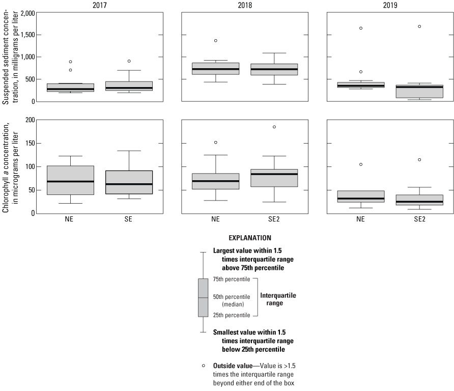
Paired distributions of suspended-sediment concentration and chlorophyll a concentration from discrete samples collected at the northeast (NE) and southeast (SE, SE2) sites, Malheur Lake, Oregon, 2017–19.
Phytoplankton and detrital material respond differently to remedial action, but the fraction of the suspended sediment that is phytoplankton cannot be determined precisely with the data collected because the stoichiometry of the cells is not known. However, some bounds can be placed on the phytoplankton percentage by assuming a reasonable range in cellular chlorophyll content. A high value of the ratio of cellular carbon to chlorophyll a (based on typical freshwater systems) might be 160 milligrams per milligram (mg/mg; Bowie and others, 1985), and a low value that is more representative of highly turbid systems could be 30 mg/mg (Geider, 1987). Combined 2017–19 CHL data from all three lake sites had a median value of 56.1 µg/L. Assuming a carbon content of 50 percent by weight in phytoplankton cells (Bowie and others, 1985), this median concentration of chlorophyll a corresponds to a possible range in phytoplankton biomass from about 18.0 mg/L at the lower cellular chlorophyll a content to 3.4 mg/L at the higher cellular chlorophyll a content. These calculations indicate that phytoplankton could comprise about 5–25 percent of the LOI, based on an LOI concentration of 73 mg/L (the median value of combined 2017–19 data from all three lake sites). Together, the relations among SSC, LOI, and CHL indicate that (1) there was a consistent organic fraction of the suspended sediment (based on the high R2 between LOI and SSC), (2) the SSC was about 18 percent organic matter (based on the median value of LOI:SSC), and (3) the organic fraction of the SSC was mostly detrital rather than phytoplankton (based on the upper bound of 25 percent phytoplankton when the highest value of carbon to chlorophyll a was assumed).
The paired distributions in figure 2 show that SSC was higher at both sites in 2018 than in 2017 and 2019; when data from both sites are aggregated for each year, pairwise Wilcoxon tests confirm that this difference is significant (p<0.001). Consistent with the finding that SSC and CHL were only weakly correlated, pairwise Wilcoxon tests on similarly aggregated data show that CHL was statistically similar in 2017 and 2018, but significantly lower in 2019. Plotting the data as time series provides additional detail and indicates that interpretation of these interannual differences is complicated by differences in sampling time frames and water depths among the 3 years (fig. 3). The differences can be moderated by normalizing SSC and CHL using depth integration (fig. 3E–3F). The normalization technique is discussed later in this section.
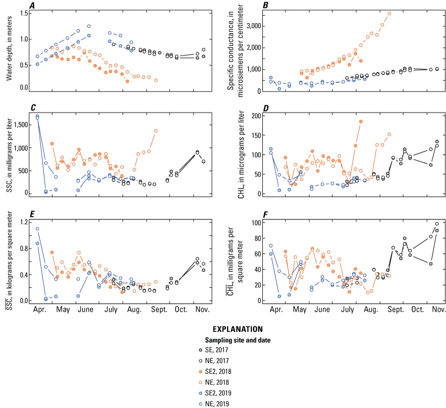
Time series plots of (A) water depth, (B) specific conductance, (C) suspended-sediment concentration (SSC), (D) chlorophyll a concentration (CHL), (E) depth-integrated suspended-sediment concentration (, and (F) depth-integrated chlorophyll a concentration () at the northeast (NE) and southeast (SE, SE2) sites, Malheur Lake, Oregon, 2017–19.
Differences in the year-to-year hydrology of the basin provide helpful context. Daily precipitation data recorded at the municipal airport in Burns, Oregon (station USW00094185; National Centers for Environmental Information, 2020), about 20 miles northwest of Malheur Lake, show that the cumulative water year precipitation as of May 1 was 28.9, 15.2, and 25.8 cm in 2017, 2018, and 2019, respectively. Winter precipitation over the lake and at the higher elevations (stored as snowpack) was much less prior to the 2018 season than it was prior to the 2017 and 2019 seasons. After the spring runoff period, lake stage in 2017 was steadily and slowly decreasing by the time sampling started in July, owing to evaporation, which can be seen in recorded water depth and field readings of specific conductance (fig. 3A–3B). At the beginning of the 2018 season (in May), lake stage was already lower than the lake stage in July 2017, and it decreased steadily through summer, as recorded in field readings of water depths and increasing specific conductance. In 2019, tributary inflows were higher for longer than in either 2017 or 2018 (reference USGS streamgage 10396000), and the lake stage increased steadily from the time sampling started in April through June, after which it declined as evaporation dominated, and specific conductance increased. The recorded water depths also show that the SE site was similar in depth to the NE site in 2017, but the SE2 site was shallower than the NE site by nearly 0.2 m in 2018.
Also notable in 2019 are the low SSC and CHL values at SE2 from mid-May through early June. These low values were a result of the high inflows of fairly clear water from the Donner und Blitzen River that affected that site in the spring of 2019 until the lake once again became spatially homogeneous. Clear water absorbs light and appears dark in imagery, whereas water with more optically active particles reflects light and appears lighter in color. The clearer water from the tributary and the subsequent mixing are visible in satellite imagery from two dates in 2019 (fig. 4).
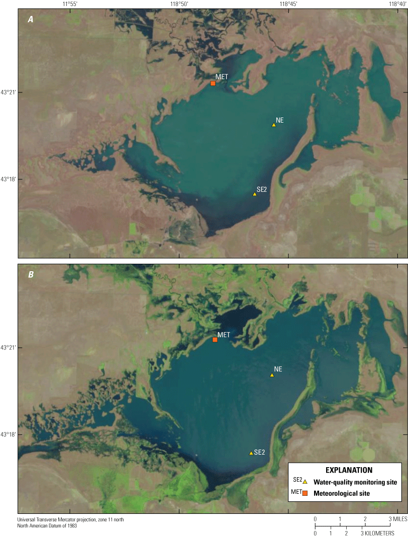
Landsat satellite images of Malheur Lake, Oregon, taken on (A) April 26, 2019, showing clearer water flowing from the Donner und Blitzen River to the southeast sampling site (SE2), and (B) June 29, 2019, showing that the water in the lake has homogenized and that water at the southeast site (SE2) is visually indistinguishable from water at the northeast site (NE).
The differences in depth can be accounted for when comparing the data by multiplying the concentrations by the water column depth—converting the data from a mass of suspended sediment in the water to a mass of suspended sediment over a unit area of the lakebed in kilograms per square meter (kg/m2; fig. 5)—as has been done in figure 3E–3F. Normalizing the data in this way (denoted by an overbar) eliminates most of the higher baseline in in 2018 compared to 2017 and 2019. Aside from low spring values at SE2 in 2019 from the effect of the Donner und Blitzen River, is largely consistent among the 3 years. The pattern that emerges is one of highest in early spring, followed by a decline through mid-summer, and another smaller increase into the autumn. values were more variable seasonally and among the 3 years than . Values of in June and July of 2018 compared to the other 2 years were still higher, but the large differences in August and September are largely removed. The seasonal cycle in is characterized by intermediate values in the spring through summer, depending on the year, and higher values into autumn. These patterns are useful for discussion purposes and provide a working hypothesis that can be tested with further data collection, but the interpretation is tentative as differences in the periods sampled make robust month-to-month comparisons difficult because spring and autumn months were not sampled in all 3 years. Discrete sample collection in 2017 and 2019 overlapped from late-June to mid-August. Discrete sampling in 2018 spanned periods from spring to summer and overlapped with both 2017 and 2019 but did not start as early as in 2019 or continue as late as in 2017.
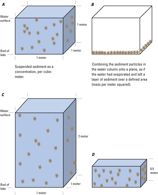
Relation between (A) volumetric concentration and (B) mass density. Mass density can be converted to an equivalent thickness of bed sediment. The volumetric concentration of sediment is determined by the mass of sediment (measured in kilograms per square meter) and the water depth (C and D); for example, at a given density, the concentration in the 0.5-meter depth (D) would be 4 times the concentration in the 2-meter depth (C).
Seasonal patterns can be clarified further with the higher temporal resolution provided by daily means from the continuous monitoring data (fig. 6A–6B). Continuous TRB was converted to SSC using equation 1 (app. 1), and then daily means of SSC and CHL were multiplied by depth to create and time series using water depth from weekly field measurements linearly interpolated to daily values (2017 and 2019) or the measured stage (2018). The lowest values of are consistent at all sites and in all years from July through October. The highest values occurred in early spring (April, except for SE2 in 2019, which was influenced by the high Donner und Blitzen River inflows), transitioning to the lowest values in summer and increasing to intermediate values in autumn (November; fig. 6A).
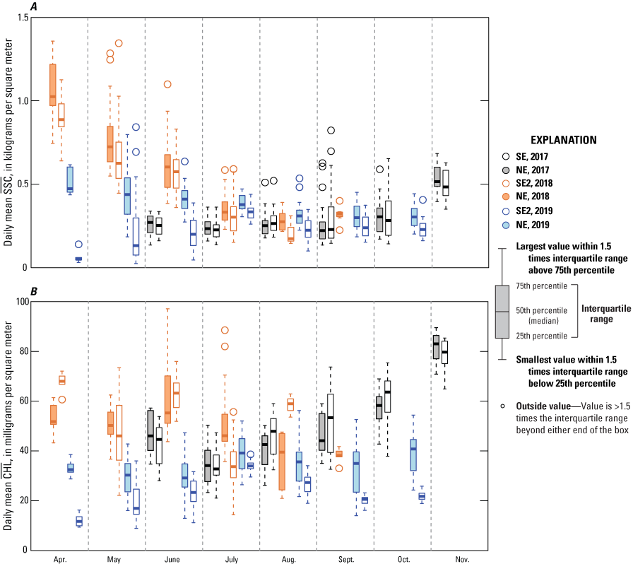
Daily means of (A) suspended-sediment density () and (B) chlorophyll a density () as a function of month in the calendar year, Malheur Lake, Oregon, 2017–19. Data are grouped by site and year. Each box contains all the daily mean suspended sediment or chlorophyll a densities from that site for that month. Water-quality monitoring sites: NE, northeast; SE, southeast; SE2, SE moved to another location.
values, in contrast to , were more variable and not characterized by a consistent seasonal pattern, although there is evidence of increasing through the autumn of 2017 (fig. 6B). Seasonal maxima occurred in November in 2017, June in 2018, and August in 2019. Again, the interpretation of seasonal dependence is tentative because spring and autumn months were not sampled in all 3 years, but a useful working hypothesis is that values are likely to be highest in spring, transitioning to lower values in summer, and increasing once again in autumn. does not lend itself to generalizations about seasonal variability, but it is notable that the seasonal patterns were moderately consistent between the northeast and southeast site in each year (except for spring of 2019 at the southeast site, owing to the influence of the Donner und Blitzen River), even though those sites were separated by 3.55 km in 2017 and 4.42 km in 2018 and 2019.
Relation Between Optically Active Particles and Wind, 2017–19
Methods of Wind Speed Data Collection
Wind speeds were measured at 30-minute intervals with an RM Young model 03002 factory-calibrated anemometer installed 3.26 m above the ground during the 2017, 2018, and 2019 sampling seasons at the Malheur Lake meteorological station located on an island near the north shore of the lake (MET station; fig. 1). Equipment failures (unrelated to weather conditions) resulted in a delayed start of data collection to August 10, 2017, and subsequent gaps of 14 days in August and 9 days November. The 2018 and 2019 datasets are complete.
Relation Between Optically Active Particles and Wind Speed—Results
The relation between and wind speed can be observed qualitatively in the daily time series (figs. 7A–7C; 8A–8C). Mass density (concentration multiplied by depth, or depth-integrated concentration) is more suitable for investigating the relation to wind and bottom shear stress than volumetric concentration because resuspension is a surface-area driven process. The depth-integrated quantities remove the effect of volume on concentration. The daily time series show that some peaks in can be visually associated with peaks in wind speed; furthermore, the pattern of peaks in is similar at the northeast and southeast sites (figs. 7 and 8), indicating a large-scale forcing function that affects both sites (wind at the surface of the lake). The Pearson correlation coefficient R between daily mean at the two sites is strongly positive (R=0.84, 3 years combined). Several peaks approaching 0.7 kg/m2 or higher are evident in 2017 on August 11, September 20, and October 8, and during November 6–9 (figs. 7A, 8A). The threshold wind speed for a response in above the background seems to be 5–10 meters per second (m/s).
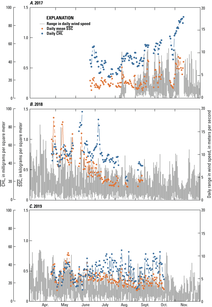
Time series of daily mean suspended-sediment density () and daily mean chlorophyll a density () at the northeast water-quality monitoring site, and the range (daily minimum to daily maximum) in wind speed at the meteorological station, Malheur Lake, Oregon, (A) 2017, (B) 2018, (C) 2019.
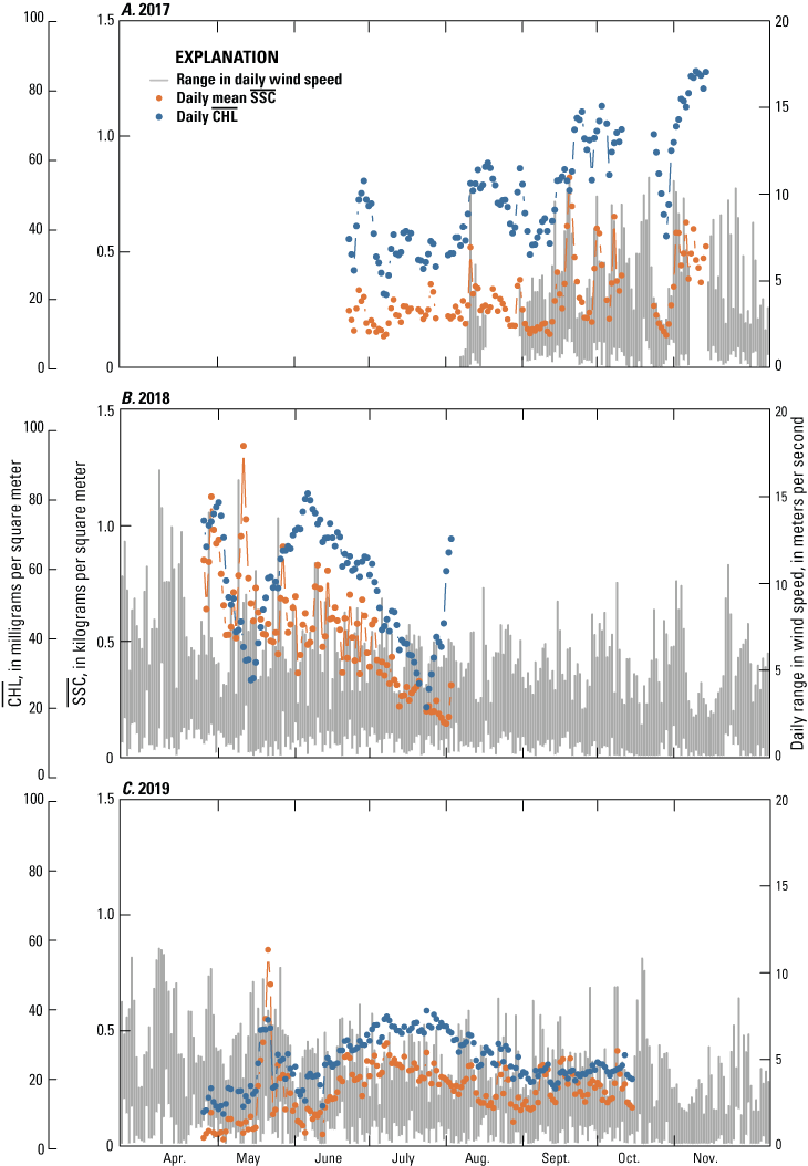
Time series of daily mean suspended-sediment density () and daily mean chlorophyll a density () at the southeast water-quality monitoring site, and the range (daily minimum to daily maximum) in wind speed at the meteorological station, Malheur Lake, Oregon, (A) 2017, (B) 2018, (C) 2019.
Spring winds at Malheur Lake are, in general, stronger than summer and autumn winds, and in spring of the 2018 sampling season (figs. 7B, 8B), several peaks in exceeded 1 kg/m2 on April 28, May 12, May 27, and June 10, again visible in the data from both sites. Peaks in wind speed associated with maxima were higher in spring; several peaks exceeded 15 m/s. Wind speeds during the spring of 2019 were lower than in corresponding months in 2018—the daily maximum wind speed exceeded 10 m/s on only 2 days in April and May—and the response in was correspondingly lower. A maximum of 0.62 kg/m2 at NE on April 30 was preceded by a daily maximum wind speed of 10.1 m/s, and another maximum of 0.8 kg/m2 on May 21 was associated with a wind maximum on May 19 of 9.5 m/s (fig. 7C). The peak on May 21 also was evident at the southeast site (fig. 8C). The peaks in at both sites and in all 3 years are consistent in that they rise in conjunction with wind events and fall within a few days when the winds subside.
Particularly in 2017, daily mean was weakly correlated with (figs. 7A, 8A). Several simultaneous peaks in the data occur in both records. The Pearson correlation coefficient between and is significant and weakly positive (R=0.46 at the northeast site, R=0.59 at the southeast site, p<0.01, 3 years combined). The reason for this correlation is not obvious, as it might be reasonable to assume that the increased turbidity associated with higher would suppress phytoplankton biomass and the associated chlorophyll rather than enhance it. Possible explanations include the suspension of benthic chlorophyll along with sediments from the bottom, or the reaction of phytoplankton to a surge in nutrients associated with the suspension of sediments. The Pearson correlation coefficient between daily mean at the two sites is strongly positive (R=0.80; p<0.01; 3 years of data combined).
The bottom shear stress was calculated from the wind-speed time series of data collected at the meteorological station, using equations from Coastal Engineering Research Center (CERC, 1984) and the depth at each site. The equations for wind-driven wave height, wavelength, and period are provided in appendix 3. These calculations require wind speed (projected to a 10-m height above land surface; see app. 3), water depth, and fetch (distance the wind blows uninterrupted across water). An approximation of fetch was determined by using measuring tools in ArcGIS (Esri, 2019). LandSat 7 and 8 georeferenced images (20-percent clouds or less) that were available during the 2017 (n=12), 2018 (n=13), and 2019 (n=13) monitoring periods were added to ArcGIS. Straight-line distances from monitoring sites to the shoreline to the north, west, and south, and to the dike to the east, were determined for each satellite image. To continue the calculations through winter, water depth and water temperature (needed for calculating water kinematic viscosity; appendix 3) were linearly interpolated from December 2017 to May 2018, and again from October 2018 to April 2019. In both winters, ice covered Malheur Lake for a period that is difficult to precisely determine, and because ice cover prevents the transfer of wind energy, the calculated shear stress is only applicable for ice-free conditions. Once the wave height, wavelength, and period are calculated, shallow-water wave theory can be used to calculate the friction factor and shear stress (app. 3).
Using these simplifications, the daily maximum of the hourly bottom shear stress was calculated for August 2017 through October 2019 (fig. 9A). The approximate range in dates each winter when the lake was covered in ice was determined by visually examining Sentinel-2 satellite imagery and are shown in figure 9A. Images are generally available at 2- to 3-day intervals, but often cloud cover obscures the lake, so dates were approximated. Bottom shear stress under ice should be nearly zero, so the calculated values are theoretical values for ice-free conditions during ice-covered conditions. The seasonal pattern in the bottom shear stress parallels wind speed, with larger values occurring in early spring (February through April) and late autumn (October and November) and lowest values occurring in mid- to late summer. During those high-wind months, daily maxima in shear stress routinely exceeded 0.3 pascals (Pa), particularly in spring, but only occasionally exceeded 0.4 Pa.
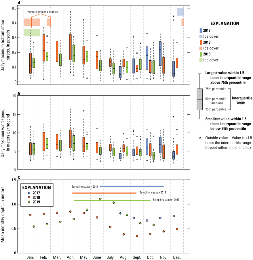
Boxplots showing (A) daily maximum bottom shear stress, aggregated by month, with the approximate duration of ice cover in each year (the calculated values of shear stress do not apply under ice cover); and (B) daily maximum wind speed, aggregated by month; and graph showing (C) mean monthly depth and the duration of the sampling season in each year, Malheur Lake, Oregon, 2017–19. Values at the northeast (NE) and southeast (SE and SE2) water-quality monitoring sites have been combined.
Another way to see the relation between bottom shear stress and on short time scales (from one to a few days) is to plot the daily maxima from each site on the same graph (fig. 10), excluding data from the southeast site in 2019 because the Donner und Blitzen River strongly affected . Only dates within the sampling season (shown in fig. 9) are included in the graph. Increasing daily maximum bottom shear stress is associated with increasing daily maximum . Pearson correlation coefficients indicate a significant linear relation (R=0.79 and 0.60 for 2017 and 2018 data, both sites combined, respectively; R=0.68 for 2019 data at the northeast site only; p<0.001 in all cases). Notably, the slope of the 2018 data is greater than the slope of the 2017 or 2019 data, even though plotting the shear stress against the depth-integrated quantity (accounts for the concentrating effect of the smaller water depth in 2018 compared to the other 2 years. In 2018, shear stress and decreased from sampling season maximum values in April to sampling season minimum values in September as the size of the lake and water depth steadily decreased (figs. 6A and 9). In contrast, in 2019 the size of the lake and water depth steadily increased from April, when measured and calculated bottom shear stresses were highest, to June, when measured and calculated bottom shear stresses leveled out (figs. 6A and 9). Continuous data collection in 2017 documented during the increase in wind speed through the autumn rather than the decrease through the spring. The measured and calculated bottom shear stresses increased steadily from August through November, during which the lake size and water depth first decreased and then increased, but the changes were smaller than in spring of 2018 and 2019 (figs. 6A and 9). Thus, decreasing lake size and water depth coincident with springtime decreasing wind speed may result in somewhat higher (as in 2018), if bottom shear stresses are similar, than increasing lake size and water depth in spring (as in 2019) or increasing wind speed in autumn (as in 2017); however, this is a working hypothesis based on limited data and would need further testing to verify.
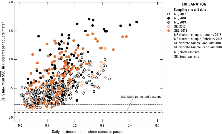
Daily maximum suspended-sediment density ( as a function of daily maximum bottom shear stress, northeast and southeast water-quality monitoring sites, Malheur Lake, Oregon, 2017–19.
Daily means of (fig. 6A) always exceeded the estimated persistent baseline of 0.11 kg/m2 of shown in figure 10, with the exception of spring 2019 data at SE2. This estimate for the persistent baseline was arrived at because it was lower than 99 percent of the daily minimum values (note that daily maximums are plotted in fig. 10) of the combined 2017–19 August and September data at the two sites. August and September data were used because those were months characterized by low winds in all 3 years, and both sites could be considered while still removing the influence of the Donner und Blitzen River on the data at SE2 in 2019 from the calculation.
Density values for two SSC samples collected in winter between the 2017 and 2018 sampling seasons are shown in figure 10. The January samples were collected by drilling a hole in 9 cm of ice cover at the NE site (the SE site was ice-free), and the February samples were collected from under about 12 cm of ice at both sites. The January samples plot below and (at the northeast site) close to the persistent baseline (), and the February samples plot above the calculated baseline but below most of the data collected during the sampling season. Thus, the few winter samples indicate that can be reduced to levels less than 0.11 kg/m2when wind action on the surface is suppressed or eliminated, but some level of , and therefore some level of turbidity because the two are related by equation 1, persists through the winter. Based on satellite imagery, the January samples (collected January 18) had been under ice since mid-December of 2017, whereas the February samples (collected on February 28) had been under ice for only about 10 days, as an ice-free period in mid-February was evident in the imagery. Some of the highest bottom shear stresses of the winter would have occurred during that February ice-free period (fig. 9), and the above baseline values measured in February may indicate that it takes several weeks for the very fine sediments responsible for to settle out of the water column after wave action is eliminated by ice.
Overall, the data provide evidence that relations between OAPs and wind strength can be considered on two time scales that correspond to different size classes of fine (less than 63 µm) sediment—a larger size class that is eroded from the bed and redeposited within a few days or less and a smaller size class that, once suspended, stays suspended for weeks. Even weak mid-summer winds or wintertime disturbance under ice cover can keep very fine particles in suspension for a long time. Therefore, represents an estimated lower bound on that is generally consistent across sites and years. The consistency suggests that the value represents a limit on imposed by the availability of the finest size class of source material.
The volumetric SSC corresponding to varies with water depth, and because SSC depends on TRB (eq. 1), the persistent turbidity (corresponding to must vary with water depth as well. Persistent turbidity as a function of water depth can be calculated by solving equation 1 for turbidity and writing SSC in the equation in terms of and water depth, and substituting for to get only the fraction of the turbidity contributed by :
whereis the water turbidity contributed by the persistent fraction of the mass density of suspended sediment, in formazin nephelometric units,
is the persistent fraction of the mass density of suspended sediment, estimated to be 0.11 kilograms per square meter, and
d
is the water depth in meters.
The relation between and water depth described by equation 2 when is set to 0.11 kg/m2 is shown in figure 11. The graphic shows how TRB measurements made by monitors or SSC measurements from discrete sample collection would vary with water depth even if wind-driven resuspension were suppressed and only the finest sediment contributing to persistent turbidity remained in suspension.
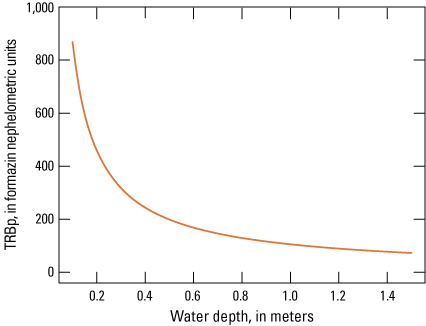
Theoretical relation between water depth and persistent turbidity (, when persistent mass density of suspended sediment is 0.11 kilograms per square meter.
Light Attenuation as a Function of Optically Active Particles
Methods of Light-Data Collection
Terrestrial Light Measurements
Incoming photosynthetically active radiation (PAR) was measured with a LI-COR LI-190R quantum sensor located at the meteorological station on an island near the north shore of the lake (fig. 1) at 30-minute intervals. Equipment malfunctions resulted in poor data quality prior to September 2017, but the quality was good from September 2017 through the end of 2018. The sensor was factory calibrated according to the manufacturer’s specifications and time intervals. Additionally, the data were checked against a clear-sky calculation and also against an AgriMet site at Prairie City, Oregon, that was at approximately the same latitude as the Malheur Lake site and also located in the high-altitude, semi-arid region east of the Cascade Range.
Underwater Light Measurements
Underwater measurements of PAR were collected (1) at 10-minute intervals at a fixed location in the water column at the northeast and southeast sites and (2) as profiles beside the deployed sensors at the northeast and southeast sites during site visits (app. 4). The profiles were collected with a factory-calibrated LI-COR LI-192 quantum sensor attached to a hand-held frame marked with depth increments (fig. 12). The quantum sensor is designed to measure PAR from wavelengths of 400 to 700 nm by filtering out shorter and longer wavelengths. The sensor measures radiation incident to a horizontal plane from all solar elevation angles. PAR is reported in units that measure the number of packets of energy, called quanta, crossing the horizontal plane in a given period of time. A quantum refers to the minimum quantity of radiation, one photon, involved in physical interactions, such as absorption by photosynthetic pigments. In this study we report PAR in micromoles photons per square meter per second (µmol/m2/s). Measurements were made just above and just below the surface and at intervals of 5 to 15 cm down to the bottom. Care was taken to position the boat such that it did not shade the profiler. These profiles were collected approximately weekly at the northeast and southeast sites.
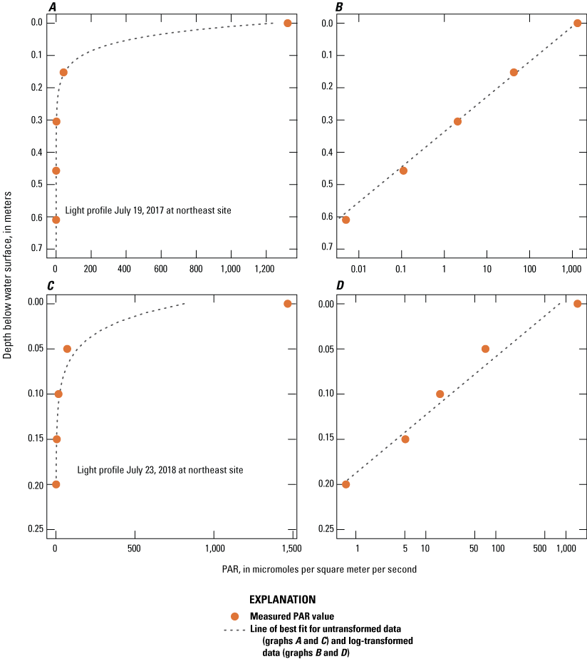
Example photosynthetically active radiation (PAR) profiles collected at the northeast site, showing exponential behavior over 20 centimeters and the best-fit line to the logarithmically transformed data, the slope of which is the attenuation coefficient, Malheur Lake, Oregon, July 19, 2017 (A and B), and July 23, 2018 (C and D).
The underwater-light time series data were collected with internally logging Odyssey PAR sensors, relatively inexpensive and self-contained PAR sensors that perform well when calibrated against a high-quality quantum sensor like the LI-COR LI-192, which was done in this case according to manufacturer instructions (Long and others, 2012). A separate wiper assembly manufactured by Zebra-Tech was installed so that the sensors would be kept relatively free of debris and biofouling between site visits. The Odyssey PAR sensors were placed on the southern side of the installation platforms in order to avoid shading by the platforms. The sensors were placed at the northeast and southeast sites in pairs to provide redundancy, but data from only one sensor at each site in any given deployment week were used to build the regression model for the attenuation coefficient.
Scaffolding installations that acted as a framework for attaching instrumentation and a platform from which to perform maintenance were constructed at the northeast (NE) and southeast (SE) sites in 2017, and again at NE and SE2 in 2018 (fig. 1; app. 4). Crews visited the sites approximately weekly to clean and check the sensors. The underwater PAR sensors were attached to a plate with a sliding collar mounted to one of the vertical supports of the installation that had been marked so that it could be used as a staff gage. The crews pulled the plate upward along the vertical support to bring it out of the water for cleaning, and then moved the plate back down to reposition the sensors once maintenance was completed, targeting a depth of about 15 cm. Crews recorded the depth of the sensors when they left the site by using the markings that were visible from the surface.
Lake stage varies over the course of a season as a result of tributary and rain inputs and evaporation losses. On shorter time scales, the surface of the lake moves vertically as weather patterns pass over and, on the shortest time scales, as wind waves progress across the surface. Incident light at the water surface in this extremely turbid environment is absorbed and scattered over a very short depth from the surface; therefore, (1) keeping the PAR sensor close to the surface and (2) determining an accurate instantaneous depth of the PAR sensor at the time of the measurement were crucial to an accurate calculation of the light attenuation coefficient. The target depth for the PAR sensors was about 15 cm. Because lake stage declines over the course of the sampling season, the sensors were placed at a target depth of 15 cm below the surface at the start of each deployment week, and they generally needed to be lowered to meet the target depth at the beginning of the next deployment week and to avoid leaving the sensor above the water surface as the lake surface lowered.
An accurate calculation of depth for the PAR sensors required two types of information: (1) the depth of the PAR sensors at the start of each deployment when the sensors were replaced at the target depth as described above and (2) subsequent changes in lake stage through time until the next site visit. Plans were made to install a recording lake-stage gage on a small island in the lake before the 2017 sampling season to record the changes in lake stage, but those plans had to be abandoned because Caspian terns (Hydroprogne caspia) and American white pelicans (Pelecanus erythrorhynchos) were nesting on the island through the spring and early summer of 2017. The changes in lake stage, therefore, were recorded by depth sensors in the YSI 6600 water-quality monitors that also were installed at the sites. Depth data collected by the monitors (at 30-minute intervals) were corrected for barometric pressure changes using barometric pressure data collected at the meteorological station on the lake for the time those measurements were available. When local barometric pressure data were not available, data from the Burns airport were used after converting the barometric pressure from the airport to local values based on a linear regression model developed with data at times when both were available. A small remaining diel-cycle variation in the depth data recorded by the water-quality monitors was removed by applying a 3-day running average to the barometric-pressure-corrected depth. To calculate a continuous depth time series for the PAR sensors, the depth was reset to the target depth recorded by the crews on the field sheets (usually 15 cm) at the beginning of each new deployment week, and the change in depth between site visits was determined by the change in depth recorded by the water-quality monitors. Linear interpolation was used to convert the measurements collected by the water-quality monitors at 30-minute intervals to the 10-minute interval of the PAR sensors.
In 2018, additional measurements were made to enable accurate positioning of the PAR sensors without an established lake-stage gage on the island. At the northeast (NE) and southeast (SE2) sites (fig. 1), lake stage was measured with an OTT HydroMet PLS pressure level sensor, and the datum for this lake stage was established with a real-time kinematic (RTK) Global Navigation Satellite System survey unit with an accuracy of plus or minus (±) 1.5 cm. The RTK survey at the sites was tied to a National Geodetic Survey monument near the refuge headquarters that has an orthometric height accuracy of ±1.6 cm. The local vertical position accuracy from RTK depended on the distance between the National Geodetic Survey monument and each site (Rydlund and Densmore, 2012). The estimated vertical accuracy of the lake stage datum was ±4.1 and ±3.8 cm at the NE and SE2 site, respectively, which was determined by summing the estimated vertical accuracy of the National Geodetic Survey monument, the instrument reported precision, and the distance-related errors (estimated at 1 part per million which computes to 1 cm for NE and 0.7 cm for SE2). The continuous depth time series of the PAR sensors was calculated in a manner analogous to that used in 2017, substituting the change in depth recorded by the OTT pressure level sensor for the change in depth recorded by the water-quality monitors.
Calculation of Clear-Sky Radiation, Reflection Coefficient, and Cloud Cover
The development of an annual time series of clear-sky radiation was used to calculate the cloud cover corresponding to measurements of incoming radiation made at the meteorological station. The clear-sky radiation at the site’s latitude and longitude, converted to PAR from full-spectrum radiation, provides a theoretical maximum for incident radiation, and deviations from that maximum can be attributed to the fraction of the sky covered by clouds. The methods to develop the time series largely followed the sequence of calculations as provided in Martin and McCutcheon (1998, p. 349–362), incorporating sunrise and sunset calculations made using the suncalc package (Thieurmel and Elmarhraoui, 2019) in the R computing environment (R Core Team, 2020). The clear-sky radiation as calculated is full-spectrum solar radiation. It was compared to daily maximum PAR data collected at the Malheur Lake meteorological station on cloudless days through 2018, and the following regression was developed to convert clear-sky full-spectrum radiation to PAR at Malheur Lake: The calculation of the reflection coefficient, based on the angle of incidence of solar radiation as a function of time of day and day in the year, also was derived from equations provided by Martin and McCutcheon (1998).
Cloud cover was calculated by comparing the hourly values of measured PAR with the theoretical maximum provided by clear-sky radiation in the PAR spectrum. Malheur Lake is located in a semi-arid climate characterized by typically sunny days during the summer; consequently, more than one-half the hourly values of cloud cover were zero. Values of measured PAR for which the calculated cloud cover was less than 20 percent, which were used to create the regression model for the attenuation coefficient, comprised 70 percent of the hourly values.
Calculation of the Attenuation Coefficient
The attenuation coefficient was calculated from the underwater PAR measurements using the following form of the Beer-Lambert law:
whereIz
is the PAR at depth z, in micromoles photons per square meter per second,
I0
is the PAR incident at the surface in the same units,
R
is the surface reflection coefficient,
B
is the surface absorption coefficient,
α
is the light attenuation coefficient, in units of per meter, and
z
is the depth below water surface, in units of meters.
Simplifying notation by defining I'0 = I0 (1 – R) (1 – B), and taking the natural log of both sides of equation 3 results in:
which shows that the natural logarithm of the measured PAR in the LI-COR profiles can be described by a straight line with a slope of α. Therefore, α was calculated from the LI-COR light profiles as the slope of a straight line fit to the log transformation of the measurements. Profile measurements deeper than 20 cm were not used in calculating the slope because deeper measurements in some profiles were affected by reflection off the bottom, creating a distortion in the profile. The slope was only calculated if at least three measurements were taken in the profile. It is also possible to rearrange equation 4 such that can be calculated from a single measurement of at a known depth:Equation 5 is used in this study to calculate the attenuation coefficient from the continuous measurements of PAR made with the Odyssey sensors and the incident light measured at the meteorological station.
Calculation of the Absorption Coefficient
Setting z = 0 in equation 3 and solving for the absorption coefficient provides the following:
whereB
is the surface absorption coefficient,
Is
is the PAR just below the water surface in micromoles photons per square meter per second,
I0
is the PAR incident at the surface in the same units, and
R
is the surface reflection coefficient.
Equation 6 was used to calculate the absorption coefficient from the LI-COR profiles. B was calculated for all profiles collected at NE and SE in 2017, and NE and SE2 in 2018, excluding the winter (January and February) samples from 2018, as well as any negative values that indicated a clear interference from clouds. The resulting distribution was normally distributed as determined by a Shapiro-Wilk normality test (p=0.45). The median value of the distribution was 0.32, which was the value of B used in the rest of the calculations.
Attenuation Coefficient as a Function of Turbidity and Chlorophyll a Concentration—Results
The minimum amount of light needed for an aquatic plant to germinate and emerge depends on factors such as plant species, temperature, and wave exposure, among others (Van den Berg and others, 1998; Penning and others, 2013). Van den Berg and others (1998) tested emergence of sago pondweed tubers at two light levels in laboratory experiments and found that emergence occurred at the lower light (36 micromoles photons per square meter per second [μmol/m2/s] PAR); evidence suggested that the lower light level was stressful and may approximate the minimum amount of light needed. Because sago pondweed is a desirable submergent macrophyte in Malheur Lake, measured PAR values were converted to a depth from the surface at which PAR was attenuated from surface values to 36 μmol/m2/s (referred to as D36 hereinafter).
The attenuation coefficient can be disaggregated into components based on the OAPs in the water or measurements that can act as surrogates for those constituents; in this study, the attenuation coefficient is modeled as a function of TRB and CHL, both of which were measured continuously:
whereα
is the light attenuation coefficient, in units of per meter,
αw
is the light attenuation coefficient of the water without OAPs,
TRB
is the turbidity, in formazin nephelometric units,
CHL
is the chlorophyll a concentration, in micrograms per liter, and
f
represents an arbitrary function.
The attenuation coefficient is often represented as a linear function of the explanatory variables, but the data collected in this study cover such a wide range of TRB and CHL values that allowing a more flexible functional form is warranted. The attenuation coefficients calculated from the time series of data from fixed underwater PAR sensors at the northeast and southeast site over 2 years were combined (fig. 13). The data used to build the regression model were restricted to values obtained when PAR sensor depths were greater than 12 cm, because at depths greater than 12 cm, the sensor is usually located below the most rapidly changing part of the light profile (fig. 12). Restricting the data in this way reduces the error in the calculated resulting from any error in the sensor depth. The data used to build the regression model also were limited to measurements collected when cloud cover was less than 20 percent, which further reduced the scatter in the data (fig. 13) by reducing error associated with the interpolation of terrestrial PAR data to the times of the underwater PAR measurements. Both the 12-cm-depth threshold and the 20-percent cloud-cover threshold were determined by trial and error, and the resulting effect on the scatter in the data was assessed visually. About 1,800 points remained in the dataset (the number varied slightly depending on which randomly chosen sensor was used from the pair at each site).
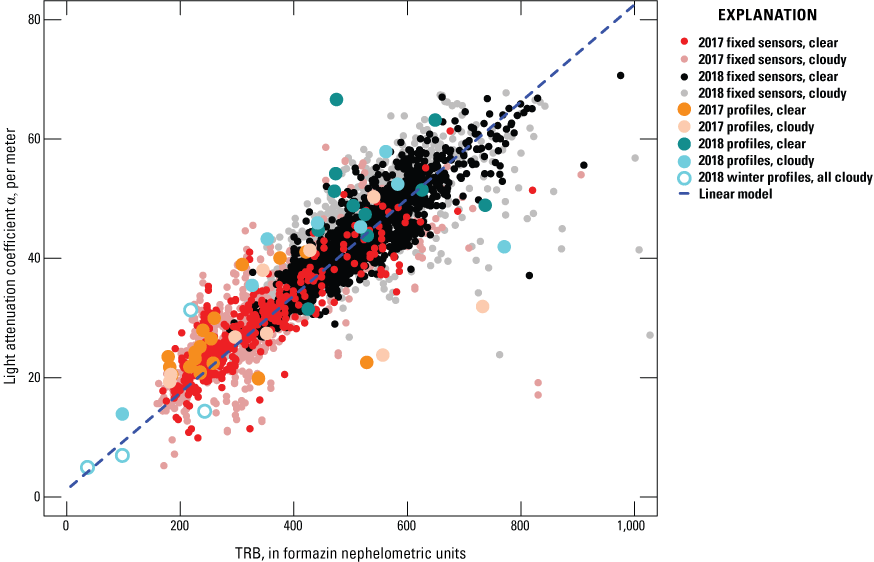
Values of light attenuation coefficient α calculated from data recorded at fixed photosynthetically active radiation sensors and from light profiles at two sites, as a function of turbidity (TRB), Malheur Lake, Oregon, 2017–18.
To eliminate inflation of the degrees of freedom in the model related to autocorrelation in turbidity or chlorophyll a concentration, 20 percent of the data was randomly subsampled (without replacement) to provide about 360 points for building a regression model. This procedure was repeated 500 times, and the coefficients from the 500 trials were averaged to get the final values (table 2). A Durbin-Watson (DW) test statistic was used to confirm that autocorrelation was eliminated. DW from all the regression models and trials was normally distributed with a mean of 2.0 and a standard deviation of 0.11 (DW varies from 0 to 4, with a value of 2 indicating no autocorrelation in the data).
Table 2.
Coefficients and error metrics for calculating the light attenuation coefficient α.[Untransformed models are in the general form of α=a+b×TRB+c×CHL, where α has units of per meter, TRB is turbidity in formazin nephelometric units, and CHL is chlorophyll a concentration in micrograms per liter. Transformed models are in the general form of ln(α)=a+b×ln(TRB)+c×ln(CHL), and BCF is a bias correction factor used to convert the expression for α from logarithmic to linear space. Italicized coefficients were not significant (p>0.1). Abbreviations and symbol: NA, not applicable; ln, natural logarithm; –, not included in model; RMSE, root-mean-squared error in units of per meter; NMRSE, root-mean-squared error divided by the interquartile range in α]
Multiple models were investigated, including linear models on the untransformed and logarithmically transformed data, models that incorporated as a fixed value, and models that allowed to be determined as the regression intercept (table 2). All the models performed moderately well (normalized root-mean-squared error from 0.26 to 0.27). Chlorophyll a concentration was tested as a predictor variable, and although it was statistically significant in one of the linear models, the addition of chlorophyll a concentration did not much improve the measurements of error. The simplest untransformed model (fig. 13) had error measurements nearly as good as any more complicated model, so the simplest untransformed model was used to calculate the depth at which light was attenuated to 36 µmol photons/m2/s in the section, “Light Attenuation by Persistent and Transient Turbidity.” This model is written:
whereα
is the light attenuation coefficient, in units of per meter,
1.2
is the value of αw in per meter,
TRB
is turbidity, in formazin nephelometric units, and
0.081
is the regression slope, in units of per meter per formazin nephelometric unit.
The value of 1.2 for αw was imposed on the linear model, based on the value used by Hostetler and Bartlein (1990). The performance of the linear model was not much degraded by imposing a known value for the y-intercept (the root-mean squared error changed from 3.47 to 3.62; table 2).
The α values calculated from profiles collected in 2017 and 2018 using the slope in equation 4 were not used to build the model but are plotted on fig.13 to show that they are consistent with the model. The magnitude of the scatter around the regression line in the values calculated from the profiles exceeds that of the values calculated from the fixed sensors. Likely explanations for the additional error in the profiles are the difficulty in maintaining a fixed position with the hand-held sensor in a moving boat while measurements were recorded, and the fact that the profile data were collected over about 20 minutes, and over that time discrete underwater PAR measurements within a single profile can be the result of changing rather than fixed conditions of TRB and incident PAR.
Measurement of Critical Shear Stress
The critical shear stress for erosion of bed sediment is an important parameter in models that simulate sediment erosion and deposition. In a large, shallow lake like Malheur Lake, the bottom shear stress is primarily caused by oscillating wave velocities at the sediment-water interface. The critical shear stress is the threshold at which the forces keeping the sediments consolidated at the bed are exceeded by forces that pull them apart, resulting in sediments that are suspended into the water above. Fine sediments are expected to behave cohesively; that is, interparticle attractions hold the particles together at the bed. The bottom shear stress must overcome these attractions for erosion and suspension to occur. A mobile erosion mini-laboratory system was used with cores collected at Malheur Lake to experimentally measure the critical shear stress.
Experimental Methods
Cores were collected from the northeast (NE) and southeast (SE2) sites in August 2018 (app. 4). An airboat transported crews to the sites and back to the mobile laboratory on the shore. Conditions at SE2 were very shallow at that time, and the cores were collected by leaning over the side of the boat to minimize disturbance of the sediments. The cores were collected by carefully pushing a clear plastic sleeve, 10 cm in diameter, about 20 cm into the sediment bed. The sleeve was much longer than 20 cm, so lake water also was collected in the sleeve above the core. A rubber disk the size of the sleeve was then pushed into the sediments to the side and underneath the sleeve, to slice and cap the core from the bottom. The cap and sleeve were pulled onto the boat and visually examined for homogeneity and signs of disturbance. The goal was to collect a core with an undisturbed, smooth, flat surface. Sometimes several attempts were made before a good quality core was obtained. At NE, where depths were greater, the method was modified by inserting the sleeve into a rubber cup attached to a long pole. The gasket provided enough suction to pull the core out of the sediments, and a second person leaned over and capped the core while it was still in the water. Two cores were collected from each site, placed into a carrier designed to minimize jostling, and transported back to shore where the mobile erosion laboratory was set up. A sample of surficial sediment was collected in duplicate at each site and sent to RTI Laboratories for the analysis of the mass fraction of water.
The experiments were performed in duplicate on the cores from each site. The theory and detailed methods for data analysis are available in Gust (1990), Gust and Mueller (1997), and Dickhudt and others (2011). The basic concept is that the water in the sleeve above the cores is capped with a rotating disk that pulls the water around the core and creates stress at the surface. The shear stress is kept nearly horizontally uniform by simultaneously pumping water radially from the outside to the center of the core. The device is calibrated so that the speed of rotation of the disk produces a known water velocity and, therefore, known shear stress at the surface.
Shear stress is applied in steps, usually starting at about 0.01 Pa, and increasing every 20–30 minutes in increments of about 0.1 Pa, to as much as about 0.6 Pa in this study. The known volume of water above the cores is continually replaced by influent with known turbidity (lake water that was collected with the cores), and turbidity is continuously measured in the effluent. Samples to be analyzed for SSC are collected from the effluent periodically and used in post-processing to calibrate the turbidity to the simultaneous mass concentration. Mass conservation is used to calculate the mass eroded at each increment of applied shear stress, and the erosion parameters including critical shear stress () are calculated using the Sanford and Maa (2001) erosion model. As the applied stress is increased at each step, the effluent turbidity increases rapidly and then slowly decreases over time to background (influent) concentration. The critical shear stress increases with distance down the core because the sediment becomes more consolidated, so each time the applied stress is increased (assuming a new critical threshold is reached), a new layer of sediment is suspended. These layers are usually on the order of fractions of a millimeter and not necessarily visible to the naked eye. Over the course of the experiment, as erosion moves down the core in thin layers, a relation between the critical shear stress and the mass eroded is obtained.
Results of Erosion Experiments
The two cores collected at the northeast site had erosion characteristics different from those collected at the southeast site (fig. 14, where the eroded mass of sediment is shown as increasing down the y-axis to be consistent with increasing depth of erosion). The mass eroded in NE cores increased much more slowly as applied shear stress was increased through time than it did in the cores from the southeast site. In fact, one of the cores from the southeast site eroded so quickly that surface changes to the core at the third increase in shear stress were visible. The eroded mass at the end of the experiments (approaching 0.6 Pa) varied by a factor of 20, from 0.06 kg/m2 at the end of the NE core 2 experiment to 1.05 kg/m2 at the end of the SE2 core 1 experiment (table 3). Care was taken while collecting the cores, and they all appeared to be of good quality (flat, uniform surface, no obvious voids), although the rapid erosion of the SE2 core 1 indicates that it may have been more heterogenous than it visually appeared to be. Therefore, the range in results likely is indicative of heterogeneity in the bottom of the lake and the different hydrologic conditions at the two sites. The NE site is located in the deepest part of the lake, which remains inundated even as the lake shrinks to its smallest extent, whereas the SE2 site is in shallower water, and the site becomes dewatered if the lake shrinks to less than about 5,000 hectares, as it did at the end of 2017 before becoming inundated again during spring runoff from the Donner und Blitzen River.
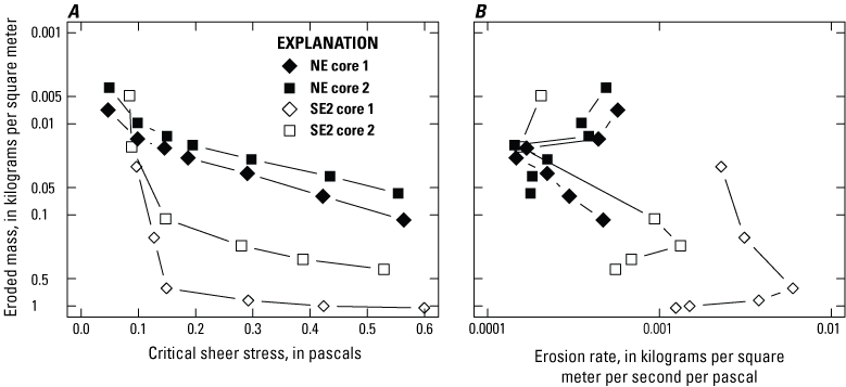
Eroded mass of cores at each step of erosion chamber experiments as a function of (A) critical shear stress and (B) erosion rate, Malheur Lake, Oregon, 2018. NE, northeast water-quality monitoring site; SE2, southeast water-quality monitoring site moved to a different location.
Table 3.
Results of mobile erosion laboratory experiments, including the mass eroded (me), the critical shear stress (), the erosion rate (M), and the depth of erosion (de), at each incremental step in the experiment.[Abbreviations and symbol: kg/m2, kilograms per square meter; Pa, pascal; kg/m2/s/Pa, kilograms per square meter per second per pascal; mm, millimeters; NE, northeast water-quality monitoring site; SE2, southeast water-quality monitoring site; –, not defined]
Two parameters useful for sediment transport models are provided in table 3: the critical shear stress (τc) and the erosion rate M (Sanford and Maa, 2001). These parameters are expected to vary with depth, and the eroded mass me in the table has been converted to an equivalent depth of eroded sediment de to support an analysis of the depth-dependence of these quantities. The conversion is:
whereρs
is the mass density of the solids in the bed, and
p
is the porosity (volume fraction of water) of the bed sediments.
A conventional value of 2,650 kg/m3 was used for , and the porosity was determined to be 0.93 at NE and 0.89 at SE2, the average of duplicate samples collected at NE and SE2. Rounding differences account for small discrepancies between the conversion between me and de calculated with equation 9, and the values of de reported in table 3. The final value of at step 8 in the experiment for the NE core 1 was 0.11 kg/m2. This mass converted to an eroded depth of 0.61 millimeters (mm). The final values of for SE2 cores 1 and 2 were 1.05 and 0.39 kg/m2, respectively, which converted to an eroded depth of 3.60 and 1.36 mm. Field personnel reported that the cores seemed to be composed primarily of an organic, peaty soil overlain by a layer of very fine, silty sediment that varied from about 1-cm thick at SE2 to 4-cm thick at NE (see report cover photograph). A layer of fine silt 1 to 4-cm thick could easily provide enough source material for the values of observed in the experiments, and for the values of observed in the lake, which reach peak values in the range of 1–1.5 kg/m2.
The results of these core experiments are not unique in the application of the mobile erosion laboratory in either the large variation among the cores or the erodibility of the sediment as measured by and M. Work and Schoellhamer (2017) reported similar variation in cores collected in the Yolo Bypass near Sacramento, California. The range in Malheur Lake cores is consistent with the range in their cores that represented nine land-use types, including two wetland types (disked and undisked), and a drain site receiving water from managed wetlands. Cores from the drain site were the most erodible in their study and most similar to SE2 cores. Malheur Lake cores cover a similar range in and M as a function of eroded mass but are more erodible when compared on the basis of the threshold required to initiate erosion. The NE cores started to erode at the second step in the experiment, at a of 0.05 Pa, and SE2 cores started to erode at 0.10 (core 1) or 0.08 (core 2) Pa. Work and Schoellhamer (2017) recorded initial values of 0.03–0.25 Pa, but only the drain site and irrigated pasture started to erode atvalues less than 0.10 Pa. Their cores were made of soils that, unlike the bottom sediments at Malheur Lake, are used for agriculture part of the year, and likely obtain some armoring when not flooded.
The critical shear stress and erosion rate coefficient of bed sediment are expected to increase as more material is eroded because the sediment becomes more consolidated with depth. Values of increase with eroded mass (the proxy for depth) in the cores (fig. 14A), but M does not increase with depth uniformly. When all cores are considered together, M seems to increase with depth, but the results of any individual core do not show this relation (fig. 14B). However, as shown in table 3, the eroded depths corresponding to the mass eroded are very small (on the order of millimeters) and when such small erosion depths are involved, lateral heterogeneity in the erosion characteristics of the bed are more important than variations with depth (Schoellhamer and others, 2017).
The erosion rate coefficient M takes on a different range of values for the NE cores compared to the SE2 cores, indicating variability in the bed sediment characteristics on scales from meters to kilometers. Furthermore, the inconsistency of M within a single core is an indication of heterogeneity in the bed characteristics at the scale of centimeters (Schoellhamer and others, 2017). The parameter values reported here provide a good beginning for a sediment transport modeling effort. A statistically robust sampling design that accounts for the various scales of heterogeneity over the large expanse of bed sediment underlying Malheur Lake would provide a better understanding of the distribution of and M; this could be especially important if future studies are concerned with the water-quality implications of suspending sediments from areas in the lake that differ based on bed sediment chemistry. Highly erodible sediments can contribute to the water quality of the lake more easily than less erodible sediments; therefore, understanding the contribution of various types of bed sediment requires some knowledge of the amount of surface area each type might represent and the erosion characteristics of each type.
Light Attenuation by Persistent and Transient Turbidity
This study has identified a potentially useful way of understanding the turbidity in Malheur Lake as the sum of a “persistent” turbidity and a “transient” turbidity. The persistent turbidity results from a baseline mass density of sediment, which we have estimated at 0.11 kg/m2. This persistent seems to be independent of wind at the surface; even in summer, when bottom shear stress often does not exceed the 0.05 to 0.1 Pa critical threshold identified in the erosion experiments, the mass density of suspended sediment remains at or above this level. This amount of suspended material also was observed in a winter sample collected under ice that had been in place about 10 days. This material is likely very fine, is released from the lakebed with minor disturbance, and remains in suspension for a long time (weeks). The persistent suspended-sediment concentration and associated turbidity increases nonlinearly as water depth decreases because the same amount of suspended mass is concentrated in a smaller volume. This effect is well-illustrated by numerical modeling of sediment resuspension in the lake (Pearson, 2020).
Transient turbidity is the result of mass eroded from and deposited on the lakebed over short time scales of one to a few days. The large variability in the mass of suspended sediment associated with transient turbidity can be directly associated with wind events that cause a bottom shear stress greater than 0.05‒0.1 Pa. The dependence of this fraction of turbidity on water depth is more complicated than the dependence of the persistent fraction. Given the same mass of resuspended material, a deeper water column results in more dilute conditions than a shallower one. Additionally, deeper water is more likely to occur in spring, when wind speeds are higher, whereas shallow water is more likely to occur late in summer after many months of evaporation, when winds are weaker. Winds tend to increase in autumn, but this can be countered in very shallow water if friction from the lakebed limits the growth of waves and, therefore, the bottom sheer stress (Pearson, 2020). Consequently, because friction in shallow water may lead to lower resuspension of transient turbidity, there is not a simple, monotonic relation between depth and turbidity; the highest turbidities may not occur with shallowest depths. When TRB from the continuous monitors at both sites are combined (with the exception of the 2019 data at the southeast site, influenced by the Donner und Blitzen River) and then disaggregated by water depth, the lowest median and highest extreme TRB values occurred at depths ranging from 0.8 to 0.9 m (fig. 15A). At depths less than 0.4 m, the TRB distribution is multimodal, with most values ranging from 700 to 1,000 FNU.
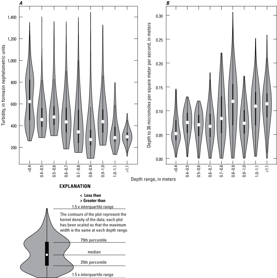
Violin plots of (A) turbidity and (B) depth of light attenuation to 36 micromoles photons per square meter per second (D36), aggregated by 0.1-meter increments of water depth, Malheur Lake, Oregon, 2017–19. Data from the northeast (NE) and southeast (SE and SE2) water-quality monitoring sites have been combined, omitting 2019 data from SE2.
Suspended sediment and turbidity are important to the lake ecosystem because they affect light attenuation, which is severe in Malheur Lake under current conditions. The very fine and mostly inorganic sediments that characterize Malheur Lake turbidity are particularly effective at light scattering (Lobo and others, 2014). Under the best conditions measured in this study, the depth of attenuation to 36 µmol photons/m2/s (D36) of incident PAR was 0.2–0.3 m. The largest median D36 occurred at depths ranging from 0.8 to 0.9 m (fig. 15B). The large range in D36 at these intermediate depths is a consequence of the great temporal variability in transient turbidity associated with wind events.
The interaction of depth, wind speed, and seasonality and the effect on D36 can be seen in figures 16 and 17. To create these figures, the time series of SSC obtained from TRB using equation 1 at the northeast site was converted to , and then the transient fraction () was calculated by subtracting a persistent of 0.11 kg/m2 from . The corresponding transient turbidity TRBt was calculated by subtracting equation 2 from equation 1, inverted to calculate TRB as a function of SSC, to get equation 10:
whereTRB
is turbidity, in formazin nephelometric units,
TRBp
is the water turbidity contributed by the persistent fraction of the mass density of suspended sediment, in formazin nephelometric units,
SSC
is suspended-sediment concentration, in milligrams per liter,
is the persistent fraction of the mass density of suspended sediment, estimated to be 0.11 kilograms per square meter, and
d
is the water depth, in meters.
α
is the light attenuation coefficient, in units of per meter,
αw
is the contribution to light attenuation by the water without TRB,
αp
is the contribution to light attenuation by persistent TRB,
αt
is the contribution to light attenuation by transient TRB,
TRBp
is the water turbidity contributed by the persistent fraction of the mass density of suspended sediment, in formazin nephelometric units, and
TRBt
is the water turbidity contributed by the transient fraction of the mass density of suspended sediment, in formazin nephelometric units.
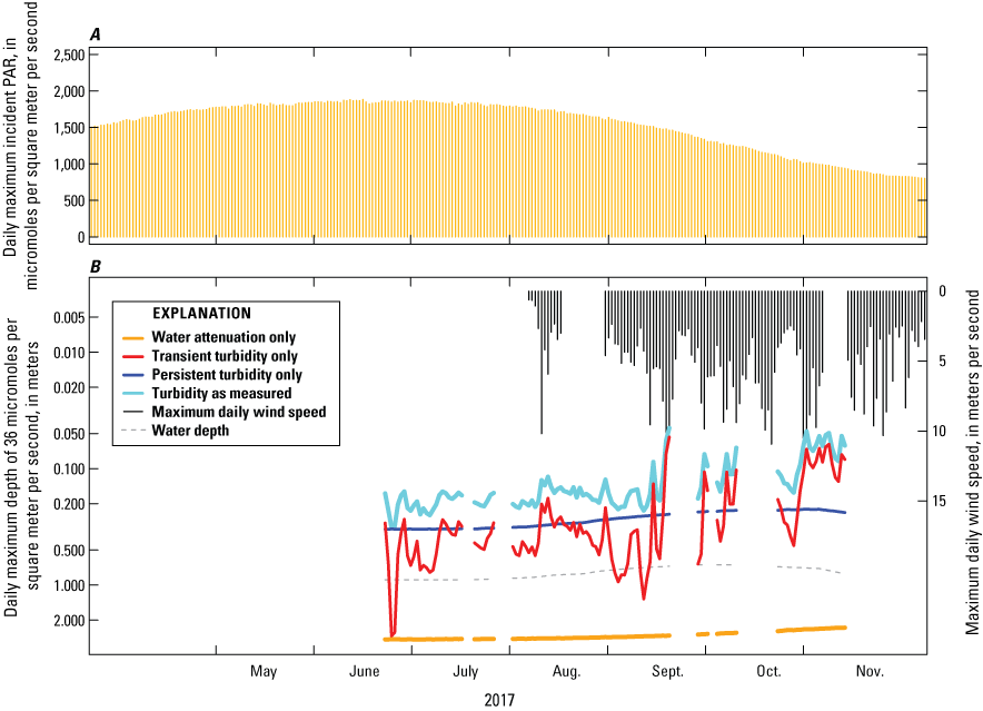
Graphs showing (A) incident photosynthetically active radiation (PAR) based on a clear-sky calculation, and (B) daily maximum wind speed and the depth at which incident PAR is attenuated to 36 micromoles photons per square meter per second (D36), Malheur Lake, Oregon, 2017. Data were collected at the northeast water-quality monitoring site and the meteorological station.
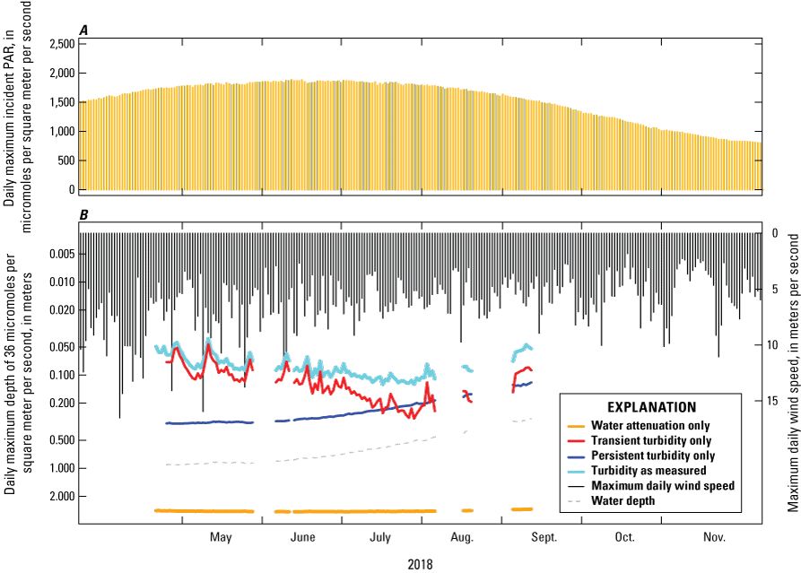
Graphs showing (A) incident photosynthetically active radiation (PAR) based on a clear-sky calculation, and (B) daily maximum wind speed and the depth at which incident PAR is attenuated to 36 micromoles photons per square meter per second (D36), Malheur Lake, Oregon, 2018. Data were collected at the northeast site and the meteorological station.
The linear model (eq. 11) was used with the turbidity corresponding to each fraction to calculate the light attenuation coefficient and its three components. The D36 was calculated using equation 3, setting Iz equal to 36 micromoles photons per square meter per second, and solving for z. The calculation was done four times, setting the attenuation coefficient α to: αw (clear water attenuation only), αp (attenuation due to TRBp only), αt (attenuation due to TRBt only), and to (attenuation due to water and total turbidity, [TRB]). A clear sky calculation converted to the PAR spectrum was used as the incident light at the surface rather than measured PAR to eliminate effects of cloud cover on the results.
Figure 16 shows that TRBp strongly and consistently attenuates light, and the D36 calculated from only TRBp never exceeded 0.4 m. As water depth decreased through the end of 2017 sampling, the D36 imposed by TRBp decreased correspondingly. The D36 calculated from only TRBt was variable and ranged from values exceeding 1 m under conditions of weak winds and low TRBt, to values less than the D36 imposed by TRBp when winds were strong and TRBt was high. Soon after data collection started, the D36 calculated from only TRBt briefly exceeded water depth, as it did on several days in September, as well. At the other end of its range, the D36 calculated from only TRBt was less than the D36 calculated from only TRBp on a few days each month, and on most days in November. The number of days that attenuation imposed by TRBt exceeded that imposed by TRBp increased later in the summer as the wind speed reached higher peaks.
Turbidity was much higher at the beginning of 2018 than at the end of 2017, and the difference can be attributed primarily to TRBt. From the beginning of data collection in 2018 through mid-July, the D36 calculated from only TRBt never exceeded the D36 calculated from only TRBp. However, water depth declined during the 2018 data collection, and by mid-summer the D36 calculated from only TRBt sometimes exceeded the D36 calculated from only TRBp, indicating that under low-wind and very shallow conditions, most of the light attenuation came from TRBp. The depth was so shallow through most of 2018 that suspended material was concentrated relative to 2017 conditions, and the range in TRBt was never as large as in 2017 and never approached the baseline attenuation of the water without turbidity, as it had (briefly) early in 2017.
For purposes of designing restoration activities, it may be useful to think in terms of two distinct sediment types contributing to total turbidity, as restoration actions targeted at transient turbidity (such as wave reduction barriers; Pearson, 2020) might differ from actions targeted at decreasing persistent turbidity (such as inducing flocculation). Because the goal is to establish emergent and submergent vegetation, it would be helpful to consider how reductions in loading of sediment from the bed would affect light attenuation. The total light attenuation coefficient can be written in terms of these quantities by combining equations 1, 2, 5, 10 and 11:
where
is the persistent mass density of suspended sediment, in kilograms per square meter,
is the transient mass density of suspended sediment, in kilograms per square meter,
is a constant equal to 1,479,
b
is a regression coefficient equal to 0.081,
d
is the water depth, in meters,
αw
is the light attenuation coefficient of the water without optically active particles, in units of per meter, and
α
is the light attenuation coefficient, in units of per meter.
The first term in curly brackets is the persistent fraction of TRB and the second is the transient fraction of TRB. Equation 12, when used in the Beer-Lambert law (eq. 3), provides a simple calculator to enable visualization of light attenuation in the three-dimensional space defined by persistent and transient sediment load and water depth (fig. 18; table 4). For the purpose of creating fig. 18 and table 4, incident light was set to the mean of the daily maximum clear sky radiation between April 15 and May 15, which was 1,759 µmol photons/m2/s, and the reflection coefficient R was set to 0, representing conditions at midday. For example, at a water depth of 1.0 m and of 0.3 kg/m2, the value of D36 is 0.12 m when is 0.11 kg/m2 (fig. 18A; table 4, row 5), and that value increases to 0.13 m if is halved (fig. 18B; table 4, row 5), or 0.16 m if is eliminated entirely (fig. 18C; table 4, row 5).
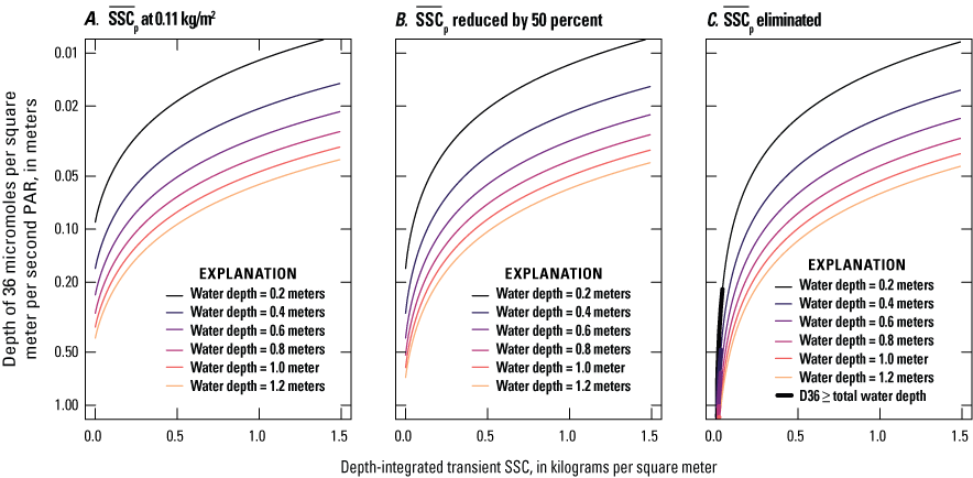
Depth at which incident photosynthetically active radiation (PAR) of 1,759 micromoles photons per square meter per second is attenuated to 36 micromoles photons per square meter per second (D36) as a function of transient sediment mass density and water depth, for (A) persistent sediment mass density () as estimated at 0.11 kilograms per square meter (kg/m2), (B) 50-percent reduction in , and (C) complete elimination of , Malheur Lake, Oregon. ≥, greater than or equal to.
Table 4.
Depth at which incident photosynthetically active radiation of 1,759 micromoles photons per square meter per second is attenuated to 36 micromoles photons per square meter per second (D36), and sediment mass density (), as a function of total water column depth (H), transient suspended-sediment mass density (), and persistent suspended-sediment mass density ().[Abbreviations: kg/m2, kilograms per square meter; m, meter]
The combined effect of the two types of sediment load is that at very high transient sediment loads associated with strong wind events, the persistent sediment load has little effect on the total sediment load and D36 (rows 13–15 in table 4). When the transient sediment load is very low, however, the effect of the persistent sediment load on total sediment load and D36 is high, and this is especially the case when the water depth is greater (rows 1–6 in table 4). In a water column of 1-m depth, D36 ranges from 0.04 to 0.36 m at an of 0.11 kg/m2, and ranges from 0.05 to 2.92 m when is eliminated entirely (rows 2, 5, 8, 11, and 14 in table 4). Because the transient sediment load is variable on short time scales and naturally varies over a wide range (represented by values on the x-axis in fig. 18 or the rows in table 4), it may make sense for restoration to prioritize reducing the persistent load, as indicated by the sequence of graphs shown in figure 18.
Other information that would inform restoration activities includes a better understanding of the composition of the sediments, particularly minerology and accurate size fractionation of the very fine sediments, to more rigorously define what this report qualitatively identifies as fractions contributing to persistent and transient turbidity. A survey of bed sediments could be useful for identifying the source of the sediment load. Our sampling design did not identify spatial differences at the sites that might indicate greater or lesser proximity to a source, but we know from satellite images that horizontal dispersion in the lake is effective at homogenizing concentrations laterally over time scales of weeks (fig. 4), and our erosion experiments identified spatial differences in the bed sediments on a kilometer scale. The source of the persistent sediments might not be ubiquitous, but limited in spatial extent, which could influence restoration alternatives.
A defining feature of Malheur Lake is the very large interannual variation in size over multiyear time scales. Our sampling covered 3 years and a range in conditions, and the size of the lake varied from a minimum of 3,420 ha at the end of 2018 to a maximum of 14,286 ha in early 2019, but this variation did not come close to capturing the entire range of normal size fluctuations that the lake has undergone in recent decades in response to climatic conditions, from 550 ha in the autumn of 1992 to about 54,320 ha in the spring of 1986 (Pearson, 2020). The implications of this large range in spatial extent for sediment load and turbidity include, but may not be limited to, the fact that water depths can be smaller and larger than we observed, and that inundating and draining large swaths of land at multiyear time scales could affect the sediment source potential of that land.
Studies that assess the effects of inundating previously exposed sediments tend to focus on the release of nutrients from the sediments when reflooded (Watts, 2000; Baldwin and Mitchell, 2000). Water quality is likely affected when previously exposed sediments are inundated. The fine particles in Malheur Lake bed sediments may aggregate and compact when dried, potentially reducing turbidity when reflooded (Fox and others, 1977; McComb and Qiu, 1998). A study by Twinch (1987) in a hypertrophic reservoir in South Africa found a 28 percent reduction of silt (or fine, 2–63 µm) material when sediments were dried, due to aggregation. However, wind-blown particles may be deposited on the exposed lakebed, potentially increasing the material available for resuspension. Dune islands in Malheur Lake provide source material for wind action and deposition, and soil cores indicate that deposition occurs during dry conditions (Dugas, 1998). It is unclear how the exposed sediments during a dry year affect sediment resuspension and turbidity in the lake; assessing compaction and wind deposition in future studies could help clarify that uncertainty. Managing exposed sediment during dry years may be one approach to lake restoration.
Summary
The high turbidity and associated high suspended-sediment concentration (SSC) of Malheur Lake in southeastern Oregon is negatively affecting the survival and propagation of desirable aquatic plants. Although the problem is evident, the composition of the turbidity and the factors affecting resuspension are multifaceted, creating a complex path toward lake restoration. This study, carried out during 2017–19, was designed to determine the types of suspended material, the erodibility of the lakebed, the attenuation of photosynthetically active radiation (PAR) through the water column, and the effects of wind and lake hydrology on SSC and turbidity.
The main types of particles that absorb or scatter light are either organic (detritus or phytoplankton) or inorganic (silt, sand, and clay). Phytoplankton is living organic matter that is autochthonously generated and remains suspended in the water column, but detritus and inorganic sediment can remain suspended or settle to the bottom and become resuspended through various processes. Lakebed-sediment samples indicated that approximately 30 percent of the top few centimeters of material was organic and >90 percent of all the material was fine material (less than 63 micrometers). Suspended-sediment samples collected from the water column had a median organic content of 18.1 percent, and 99–100 percent of all material was fine material. The high concentrations of fine material in the water column can be expected to strongly attenuate light.
Other than in 2019 when water from the Donner und Blitzen River influenced the southeast site, data (SSC and chlorophyll a concentration) collected from two locations in the lake were not significantly different, suggesting that the concentration of optically active particles (material suspended in the water that absorbs and [or] scatters light) at the two locations is largely a result of a large-scale forcing that affects both sites. Resuspension from bottom shear stress associated with wind-driven waves is an example of such a large-scale forcing. Results indicate that the organic fraction of the suspended material is mostly detritus rather than phytoplankton, assuming a reasonable range in chlorophyll a cellular stoichiometry. SSC was significantly higher at both sites in 2018 compared to comparable sampling dates in 2017 and 2019, and the interannual differences were mostly due to the lower amount of precipitation in 2018, which resulted in shallower lake depths. Combining 3 years of SSC values multiplied by water depth () shows a seasonal pattern: concentrations are often highest in early spring, lowest in summer, and intermediate in autumn. Seasonal patterns are not consistent for chlorophyll a concentration values.
Turbidity, a surrogate for SSC, was measured continuously with a water-quality monitor. A relation was developed to convert turbidity to SSC, which was compared to wind speed measured at a nearby meteorological station. Wind speeds tend to be strongest in spring and weakest in summer, but they vary substantially. Wind speeds of 5–10 meters per second (m/s) caused rapid increases in turbidity readings above background that lasted for a few days. Between strong wind events, and during extended periods of low winds, calculated from turbidity and depth did not decrease to near-zero values, but instead had a lower bound indicating a baseline, or persistent, representing a fixed suspended mass of sediment that is independent of wind speed. These observations supported the partitioning of turbidity (and SSC) in Malheur Lake into transient and persistent components.
Because is multiplied by water depth, the persistent baseline of p) is independent of water depth. When p) is converted tvolumetric concentration (SSC), however, the baseline concentration decreases with increasing water depth, indicating that the fixed suspended mass of sediment over a given area (estimated to be 0.11 kilograms per square meter) is spread over a deeper water column. Because SSC and turbidity have a one-to-one correspondence and increase together, the turbidity corresponding to the persistent baseline volumetric concentration also decreases with increasing water depth.
The critical shear stress required to suspend bottom sediment was measured with erosion experiments on sediment cores collected from the lake. Based on these experiments, transient turbidity is initiated by wind events that exceed about 0.05 to 0.1 Pa in bottom shear stress. The erosion experiments indicated variability in the critical shear stress required to release the bottom sediments from the two lake sites; however, much of the lakebed likely is highly erodible. Some of the variability in bottom sediments may be related to seasonal inundation and whether the sediment at that location was exposed to air the previous year. The highest turbidities may not occur at the shallowest lake depths because of the effect of friction on wind-wave development and associated bottom shear stress and sediment resuspension. Persistent turbidity remains when bottom shear stress is less than 0.05 Pa and, because of its very fine grain size, strongly and consistently attenuates light. Transient turbidity will cause additional light attenuation, depending on depth and wave action resulting from wind stress.
The attenuation of PAR with depth as a function of turbidity was determined by using a robust linear regression model that included data recorded by terrestrial and underwater PAR sensors. This attenuation coefficient can be used in modeling restoration scenarios, and it was used in this study to examine the contributions of persistent and transient turbidity to light attenuation independently.
Restoration actions may target the persistent or transient turbidity. For example, wave-reduction barriers may reduce transient turbidity, and flocculation may affect the persistent turbidity. Some strategies, such as reducing exposed sediments during dry years through greater plant coverage, likely will affect both turbidity components. A consideration in restoration is that transient turbidity naturally varies over a wide range, whereas persistent turbidity imposes a consistent limit on PAR transmission to the bed. For example, under current conditions, the depth at which an average daily maximum of incident PAR (between April 15 and May 15) is attenuated to 36 micromoles photons per square meter per second (µmol photons/m2/s) varies from 4 to 36 centimeters (cm) when the water is 1 m deep, whereas if the persistent turbidity were reduced by one-half, the depth at which incident PAR is attenuated to 36 µmol photons/m2/s varies from 4 to 61 cm. Lowering the persistent turbidity has the potential to enable transmission of light much deeper into the water column during times of weak winds when the transient turbidity is low.
Ideally, restoration actions will lead to a positive feedback loop, in which reductions in turbidity lead to the establishment of vegetation in parts of the lake where depth, bottom characteristics, and wind-wave conditions are most favorable. These reductions, in turn, could potentially reduce resuspension in these locations, reduce the source of resuspended material to the lake as a whole, and interrupt wind-wave development, thus further reducing turbidity and allowing vegetation to establish in an increasing areal extent, eventually leading to a clear and highly vegetated system.
References Cited
Bowie, G.L., Mills, W.B., Porcella, D.B., Campbell, C.L., Pagenkopf, J.R., Rupp, G.L., Johnson, K.M., Chan, P.W.H., Gherini, S.A., and Chamberlin, C.E., 1985, Rates, constants, and kinetics formulations in surface water quality modeling: U.S. Environmental Protection Agency, Report No. EPA/600/3-85/040, 455 p.
Chen, Y., Qin, B., Teubner, K., and Dokulil, M.T., 2003, Long-term dynamics of phytoplankton assemblages—Microcystis-domination in Lake Taihu, a large shallow lake in China: Journal of Plankton Research, v. 25, no. 4, p. 445–453. [Also available at https://doi.org/10.1093/plankt/25.4.445.]
Dokulil, M., 1984, Assessment of components controlling phytoplankton photosynthesis and bacterioplankton production in a shallow, alkaline, turbid lake (Neusiedlersee, Austria): Internationale Revue der Gesamten Hydrobiologie und Hydrographie, v. 69, p. 679–727. [Also available at https://doi.org/10.1002/iroh.19840690506.]
Esri, 2019, ArcGIS online: Esri, accessed October 1, 2021, at https://www.esri.com/en-us/landing-page/product/2019/arcgis-online/overview.
Fox, J.L., Brezonik, P.L., and Keirn, M.A., 1977, Lake drawdown as a method of improving water quality: U.S. Environmental Protection Agency Report No. EPA-600/3-77-005, 93 p., accessed September 24, 2020, at https://nepis.epa.gov/Exe/ZyPDF.cgi/9101QX6N.PDF?Dockey=9101QX6N.PDF.
Guang, J., Wei, Y., and Huang, J., 2006, A model for the retrieval of suspended sediment concentrations in Taihu Lake from TM images: Journal of Geographical Sciences, v. 16, p. 458–464. [Also available at https://doi.org/10.1007/s11442-006-0409-3].
Gust, G., and Mueller, V., 1997, Interfacial hydrodynamics and entrainment functions of currently used erosion devices, in Burt, N., Parker, R., and Watts, J. eds., Cohesive sediments, 4th Nearshore and estuarine cohesive sediment transport conference INTERCOH '94 [Proceedings], July 11–15, 1994, Wallingford, United Kingdom: New York, Wiley, p. 149–174.
Lobo, F., Costa, M., Phillips, S., Young, E., and McGregor, C., 2014, Light backscattering in turbid freshwater—A laboratory investigation: Journal of Applied Remote Sensing, v. 8, no. 1, p. 083611, accessed on January 11, 2022, at https://doi.org/10.1117/1.JRS.8.083611.
McComb, A., and Qiu, S., 1998, The effects of drying and reflooding on nutrient release from wetland sediments, in Williams, W.D., ed., Wetlands in a dry land—Understanding for management: Canberra, Australia, Environment Australia, p. 147–159. [Also available at https://researchrepository.murdoch.edu.au/id/eprint/23906/.]
National Centers for Environmental Information, 2020, Looking for data?: National Centers for Environmental Information web page, accessed August 21, 2020, at https://www.ncei.noaa.gov/.
Pascolo, S., Petti, M., and Bosa, S., 2018, On the wave bottom shear stress in shallow depths—The role of wave period and bed roughness: Water, v. 10, 19 p., accessed March 9, 2022, at https://doi.org/10.3390/w10101348.
R Core Team, 2020, The R project for statistical computing: Vienna, Austria, The R Foundation web page, accessed January 10, 2020, at http://www.r-project.org.
Rydlund, P.H., Jr., and Densmore, B.K., 2012, Methods of practice and guidelines for using survey-grade global navigation satellite systems (GNSS) to establish vertical datum in the United States Geological Survey: U.S. Geological Survey Techniques and Methods, book 11, chap. D1, 102 p. with appendixes.
Schoellhamer, D., Manning, A., and Work, P., 2017, Erosion characteristics and horizontal variability for small erosion depths in the Sacramento-San Joaquin River Delta, California, USA: Ocean Dynamics, v. 67, no. 6, p. 799–811. [Also available at https://doi.org/10.1007/s10236-017-1047-2.]
Smith, C.D., 2022, Phytoplankton data for Malheur Lake, Oregon, 2018–20: U.S. Geological Survey data release, accessed January 3, 2022, at https://doi.org/10.5066/P92ZBWJ5.
Thieurmel, B., and Elmarhraoui, A., 2019, Package 'suncalc'—The R project for statistical computing: Vienna, Austria, The R Foundation web page, accessed August 15, 2020, at http://www.r-project.org/.
U.S. Fish and Wildlife Service, 2012, Refuge waters in peril: U.S. Fish and Wildlife Service, 4 p., accessed July 22, 2015, at https://permanent.access.gpo.gov/gpo30861/AQ_Health_brochure_1.pdf.
U.S. Geological Survey, 2016: U.S. Geological Survey, Office of Surface Water Technical Memorandum 2016.07, 40 p., accessed February 10, 2021, at https://vdocument.in/united-states-department-of-the-interior-usgs-wq201610pdf-united-states-department.html.
U.S. Geological Survey, 2018, General introduction for the “National Field Manual for the Collection of Water-Quality Data” (ver. 1.1, June 2018): U.S. Geological Survey Techniques and Methods, book 9, chap. A0, 4 p., accessed January 11, 2022, at https://doi.org/10.3133/tm9A0. [Supersedes U.S. Geological Survey Techniques and Methods, book 9, chap. A0, version 1.0.]
U.S. Geological Survey, 2020, USGS water data for the Nation: U.S. Geological Survey National Water Information System database, accessed September 10, 2020, at https://maps.waterdata.usgs.gov/mapper/index.html.
U.S. Geological Survey, 2022, USGS data grapher and Data tabler: U.S. Geological Survey Oregon Water Science Center web page, accessed January 11, 2022, at https://or.water.usgs.gov/grapher/.
Wagner, R.J., Boulger, R.W., Jr., Oblinger, C.J., and Smith, B.A., 2006, Guidelines and standard procedures for continuous water-quality monitors—Station operation, record computation, and data reporting: U.S. Geological Survey Techniques and Methods, book 1, chap. D3, accessed February 1, 2017, at https://pubs.water.usgs.gov/tm1D3.
Wood, T.M., 2022, Photosynthetically active radiation measurements collected at Malheur Lake, Oregon, 2017–18: U.S. Geological Survey data release, https://doi.org/10.5066/P95FMN8F.
Appendix 1. Model Development and Documentation—Suspended-Sediment Concentrations and Turbidity Measurements
Model
logssc = + 1.09 * logturb - 0.174
where
ssc	is suspended-sediment concentration, in milligrams per liter, and
turb	is turbidity, in formazin nephelometric units.
Variable Summary Statistics
             logssc  ssc logturb turb
Minimum        2.29  195    2.26  180
1st Quartile   2.48  304    2.46  290
Median         2.77  587    2.69  484
Mean           2.70  569    2.63  471
3rd Quartile   2.89  773    2.76  580
Maximum        3.14 1370    3.00 1010
Basic Model Statistics
Number of observations:                             58
Standard error (RMSE):                          0.0696
Average Model standard percentage error (MSPE):   16.1
Coefficient of determination (R2):               0.912
Adjusted Coefficient of determination (Adj. R2): 0.911
Bias Correction Factor (BCF):                     1.01
Explanatory Variables
            Coefficients Standard Error t value Pr(>|t|)
(Intercept)       -0.174         0.1190   -1.46 1.51e-01
logturb            1.090         0.0453   24.10 2.85e-31
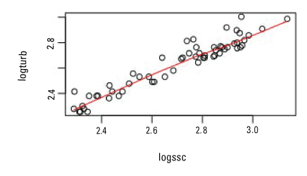
Log-transformed suspended-sediment concentrations (logssc; in milligrams per liter) and log-transformed turbidity values (logturb; in formazin nephelometric units). Model (diagonal line) was developed from samples and measurements (circles) collected in Malheur Lake, Oregon, 2017–18.
Appendix 2. Model Development and Documentation: Continuous Chlorophyll Fluorescence Sensor Readings and Chlorophyll a Concentrations
NWIS Site Information
Northeast (NE)
NWIS Site ID: 432004118453400
NWIS Site Name: Malheur Lake – MAL-NE
Sampling Location: The site is located at 43°20'4.31"N, 118°45'34.10"W within the Malheur National Wildlife Refuge, Oregon.
Monitoring Dates: Seasonally in 2017, 2018, and 2019
Site characteristics: Malheur Lake is a vast, shallow, turbid lake in southeast Oregon. Aquatic plants only exist on the lake margins and the lake contains non-native carp. The northeast site (NE) in the lake is inundated all year and is usually approximately 1 meter deep. The water column is fairly well-mixed from the surface to the sediment.
Southeast (SE)
NWIS Site ID: 431826118465600
NWIS Site Name: Malheur Lake – MAL-SE
Sampling Location: The site is located at 43°18'25.95”N, 118°46'55.71”W within the Malheur National Wildlife Refuge, Oregon.
Monitoring Dates: Summer and autumn 2017
Site Characteristics: This site has very similar conditions to the NE site.
Southeast 2 (SE2)
NWIS Site ID: 431745118462300
NWIS Site Name: Malheur Lake – MAL-SE 2
Sampling Location: The site is located at 43°17'45.4”N, 118°46'22.6”W in Malheur Lake within the Malheur National Wildlife Refuge, Oregon.
Monitoring Dates: Seasonally in 2018 and 2019
Site Characteristics: The southeast water-quality monitoring site moved to a different location (SE2) in the lake becomes inundated in the spring and is usually less than 1 meter deep. The water column is fairly well-mixed from the surface to the sediment. During wet water years, this site is largely influenced by the Donner und Blitzen River in spring, and turbidity is low during that time. Later in the season, the site is similar to the NE site.
Water-Quality Monitor Information (Applicable to All Sites and Years)
YSI 6600 multiparameter water-quality monitors were deployed horizontally in the middle of the water column; monitors were repositioned to mid-depth at each site visit. In 2017 and 2018, deployed monitors were exchanged with clean and calibrated monitors at site visits. In 2019, the deployed monitor was not exchanged at site visits. Instead, the monitor was taken to the refuge biology laboratory for recalibration and was redeployed the following day. Both site visit methods (exchanging monitors and recalibrating the same monitor) are valid; however, exchanging monitors may result in the need for additional corrections while recalibrating the same monitor results in missing data. Fouling and calibration corrections were applied following Wagner and others (2006).
The YSI 6025 chlorophyll sensor was calibrated with a two-point calibration to deionized water and a diluted rhodamine water tracer standard solution. The concentrated rhodamine water tracer standard was diluted to 200:1, creating a 0.625 mg/L solution. The calibration value entered into the monitor software was based on a temperature-compensated table in the YSI manual. Recalibration was performed if the sensor value differed from the table value by ±5 percent when checked in standards. The monitors logged chlorophyll readings in micrograms per liter and relative fluorescence units.
Conversion of Chlorophyll Fluorescence Sensor Readings to Chlorophyll a Concentrations
Based on multiple years of data (2017–19), multiple sites (NE, SE, SE2), and microscopy samples, very large differences in chlorophyll occur year-to-year and sometimes site-to-site, likely because of differences in the phytoplankton population (Smith, 2022). Information is not available about the phytoplankton community in 2017, and there is little information about the phytoplankton community in 2018 because only one reconnaissance sample was collected at both sites (NE and SE2) in mid-August. In 2019, chlorophyll a and microscopy samples were collected every other week from late April through mid-August. Distinct differences in the phytoplankton community can be seen, particularly at SE2 but also at NE to a lesser extent, in the August 2018 samples compared to any sample collected in 2019. At the SE2 site in August 2018, the sample was dominated by cyanobacteria in the micro-size range (the largest), and the biovolume total was greater than anything measured in 2019. At NE, the difference between August 2018 and 2019 samples was not nearly as extreme. Therefore, the unusual chlorophyll pattern in 2018 at SE2 was likely real and due to differences in the phytoplankton community. Multiple plots were created for the 3 years of data and 3 sites to assess relations between chlorophyll sensor fluorescence (in micrograms per liter [µg/L]) measured by the deployed water-quality monitor and chlorophyll a concentrations (µg/L) in the corresponding discrete water samples.
NE 2017 and SE 2017 Chlorophyll a Regression
Regression: y = 2.1455x–25.109; coefficient of determination (R2) =0.8192
Based on the comparisons (by year, by site, and combined), the 2017 data combined from both the NE and SE sites created a logical regression (R2=0.82; standard error of the estimate= 13.98). The linear regression applied to the 2017 data and the 95-percent prediction intervals are shown in figure 2.1. Figure 2.2 shows the 2017 “Chlorophyll a, regress” time series at NE, and figure 2.3 shows the 2017 “Chlorophyll a, regress” time series at SE. These time series should be considered the final, computed chlorophyll a datasets and are available in NWIS—Web Interface (U.S. Geological Survey, 2020). In both figures 2.2 and 2.3, the discrete laboratory sample values plot along the final datasets and support the chosen regression.
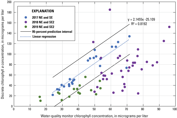
Chlorophyll concentrations measured with a water-quality monitor and chlorophyll a concentrations measured in corresponding discrete water samples collected from northeast (NE) and southeast (SE and SE2) sites in Malheur Lake, Oregon, 2017–19. Discrete samples were analyzed at the U.S. Geological Survey National Water Quality Laboratory. Linear regression includes the 2017 NE and SE site data.
Final continuous chlorophyll a dataset and discrete chlorophyll a laboratory sample values for northeast (NE) water-quality monitoring site in Malheur Lake, Oregon, 2017.
Final continuous chlorophyll a dataset and discrete chlorophyll a laboratory sample values for southeast (SE) water-quality monitoring site in Malheur Lake, Oregon, 2017.
NE 2018 and NE 2019 Chlorophyll a Regression
Regression: y = 0.0254x1.8587; R2=0.8109
Based on the comparisons (by year, by site, and combined), a regression including data from NE in 2018 and NE in 2019 created a logical regression (R2= 0.81; standard error of the estimate= 13.70). NE values in 2019 were generally low, whereas NE values in 2018 were high; therefore, a regression with both years expands the laboratory sample range and allows for interpolation rather than extrapolation. The regression is a power function which keeps the low predicted values in 2019 greater than zero. The power regression applied to the NE 2018 and NE 2019 data and the 95-percent prediction intervals are shown in figure 2.4. Figures 2.5–2.6 show the “Chlorophyll a, regress” time series at NE in 2018 and 2019, respectively. These time series should be considered the final, computed chlorophyll a datasets. The discrete laboratory sample values follow the pattern and general magnitude of the final datasets, which support the chosen regression. In 2019, the first discrete sample in April was collected before the continuous monitor was deployed (fig. 2.6).
Graph showing chlorophyll concentrations measured with a water-quality monitor and chlorophyll a concentrations measured in corresponding discrete water samples collected from northeast (NE) and southeast (SE and SE2) water-quality monitoring sites in Malheur Lake, Oregon, 2017–19. Discrete samples were analyzed at the U.S. Geological Survey National Water Quality Laboratory. Power regression includes the data from the NE site in 2018 and 2019.
Graph showing final continuous chlorophyll a dataset and discrete chlorophyll a laboratory sample values for northeast (NE) water-quality monitoring site in Malheur Lake, Oregon, 2018.
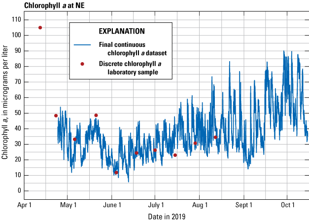
Graph showing final continuous chlorophyll a dataset and discrete chlorophyll a laboratory sample values for southeast (NE) water-quality monitoring site in Malheur Lake, Oregon, 2019.
SE2 2018 Chlorophyll a Regression
Regression: none
At the SE2 site in 2018, a single regression was not applied to the dataset due to various sensor responses throughout the season. Instead, Set 3 corrections (“other” corrections) were applied in segments to adjust the chlorophyll a time series values in micrograms per liter to match the concentrations of discrete samples collected in the field. The chlorophyll a value from the deployed monitor at the closest time to the sample collection time was used to calculate a ratio. In cases where the sample was collected between two logged values, an average of the two values bracketing the sample collection time was used. For this analysis period, Set 3 corrections began with the April 20–May 1, 2018, period. Discrete samples showed a wide range of ratios compared to the monitor values for the duration of the deployments; therefore, some corrections were applied between site visits, and some corrections spanned multiple visits if the ratios were similar. The two highest chlorophyll a sample concentrations occurred at the last two site visits of the sampling season, and the monitor data were adjusted to the ratios for the two site visits. The ratio calculated on May 29, 2018, was not used because the sample concentration from that day matched the monitor values after the ratio for June 5, 2018, was applied. Figure 2.7 shows the 2018 “Chlorophyll a, regress” time series at SE2 and is the final, computed chlorophyll a dataset available in NWIS—Web Interface (U.S. Geological Survey, 2020).
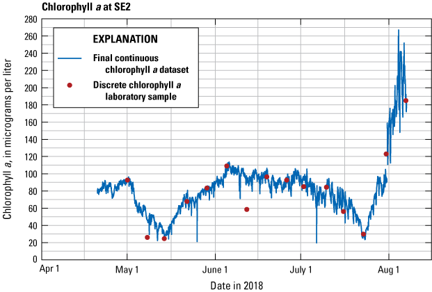
Graph showing final continuous chlorophyll a dataset and discrete chlorophyll a laboratory sample values for southeast (SE2) water-quality monitoring site in Malheur Lake, Oregon, 2018.
SE2 2019 Chlorophyll a Regression
Regression: none
Based on the sensor and discrete sample comparisons (by year, by site, and combined), it was decided that a regression was not needed for the SE2 2019 data. Some regressions were attempted, but they forced the continuous data negative. The laboratory sample values plot closely along the corrected continuous fluorescence data and applying a regression (a correction) would not remove any bias. Figure 2.8 shows the 2019 “Chlorophyll a, regress” time series at SE2. This time series should be considered the final, computed chlorophyll a dataset and is available in NWIS—Web Interface (U.S. Geological Survey, 2020). The discrete laboratory sample values follow the pattern and general magnitude of the final dataset, which supports the decision not to apply a regression.
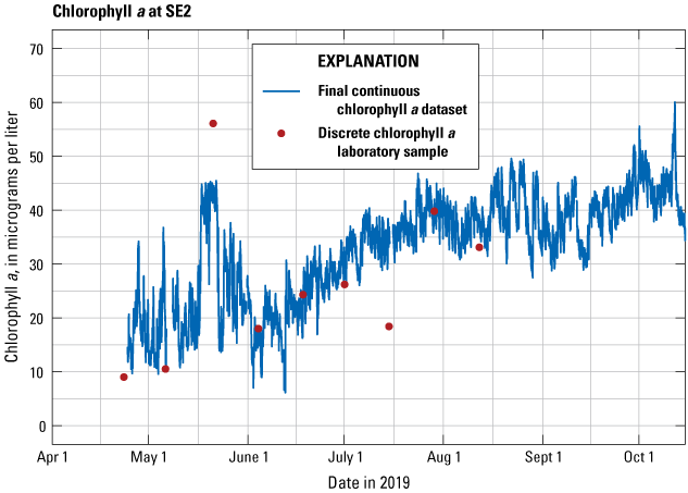
Graph showing final continuous chlorophyll a dataset and discrete chlorophyll a laboratory sample values for southeast (SE2) water-quality monitoring site in Malheur Lake, Oregon, 2019.
Appendix 3. Equations used in Calculation of Bottom Shear Stress
U
is the wind speed in meters per second at a height of 10 meters, and
g
is the acceleration due to gravity (9.8 meters per second squared).
is the roughness height, set equal to .001 meter,
U
is the wind speed at 10-m height above land surface,
U3.26
is the wind speed at 3.26-m height above land surface, and
ln
is the natural logarithm of x.
is the kinematic viscosity of water, in square meters per second, which is related to the absolute viscosity of water by .
Appendix 4. Photographs Showing Equipment Installations and Mobile Erosion Laboratory, Malheur Lake, Oregon
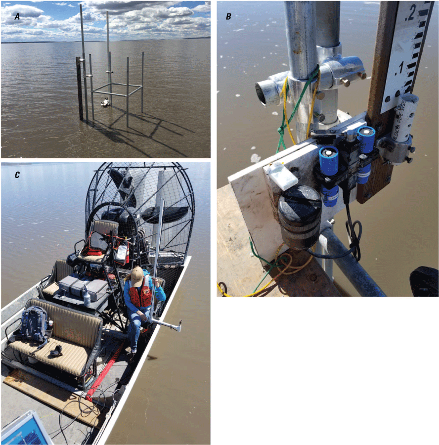
Photographs showing (A) one of the scaffolding installations for lake data collection, (B) Odyssey photosynthetically active radiation (PAR) sensors with Zebra-Tech wiper attached to moveable plate on scaffolding, and (C) the LI-COR LI-192 quantum sensor attached to a hand-held frame marked with depth increments, used to collect PAR profiles, in Malheur Lake, Oregon. Photograph A by Andrew Erickson, U.S. Geological Survey. Photographs B and C by Joe Barnett, U.S. Fish and Wildlife Service.
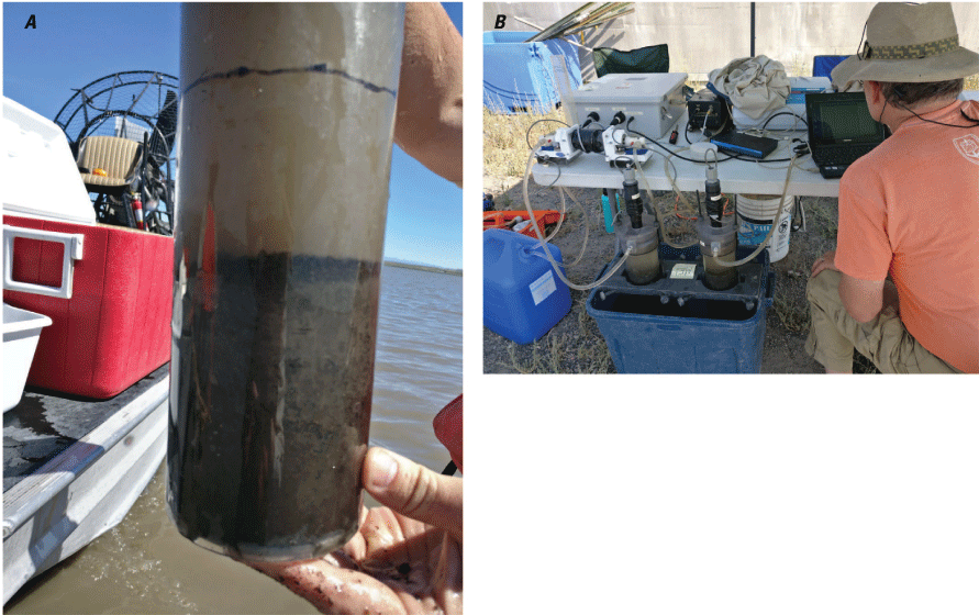
Photographs showing (A) one of the sediment lake cores collected in August 2018 and (B) the mobile erosion laboratory setup on land, at Malheur Lake, Oregon. Photographs by Joe Barnett, U.S. Fish and Wildlife Service.
Conversion Factors
International System of Units to U.S. customary units
Temperature in degrees Celsius (°C) may be converted to degrees Fahrenheit (°F) as follows:
°F = (1.8 × °C) + 32.
Supplemental Information
Specific conductance is given in microsiemens per centimeter at 25 degrees Celsius (µS/cm at 25°C).
Concentrations of suspended sediment and loss on ignition in water are given in milligrams per liter (mg/L), and concentrations of chlorophyll a in water are given in micrograms per liter (µg/L). Continuous and discrete water-quality data collected during this study are available online in the National Water Information System (NWIS; U.S. Geological Survey, 2020). Photosynthetically active radiation data and the associated water depths of the measurements, as time series and as profiles, are available in Wood (2022). Statistical test calculations were performed using the basic statistics package in the R computing environment (R Core Team, 2020).
Abbreviations
ANCOVA
analysis of covariance
CERC
Coastal Engineering Research Center
CHL
chlorophyll a concentration
chlorophyll a concentration multiplied by water depth
DW
Durbin-Watson
FNU
formazin nephelometric unit
LOI
loss on ignition
NE
northeast water-quality monitoring site
NWIS
National Water Information System
OAP
optically active particle
p
probability in a statistical test that the null hypothesis is true
PAR
photosynthetically active radiation
R
Pearson correlation coefficient
R2
coefficient of determination
SE
southeast water-quality monitoring site
SE2
southeast water-quality monitoring site moved to a different location
SSC
suspended-sediment concentration
suspended-sediment concentration multiplied by water depth
persistent fraction of
transient fraction of
TRB
turbidity
TRBp
persistent fraction of turbidity
TRBt
transient fraction of turbidity
USGS
U.S. Geological Survey
Publishing support provided by the U.S. Geological Survey
Science Publishing Network, Tacoma Publishing Service Center
For more information concerning the research in this report, contact the
Director, Oregon Water Science Center
U.S. Geological Survey
2130 SW 5th Avenue
Portland, Oregon 92701
Suggested Citation
Wood, T.M., and Smith, C.D., 2022, Light attenuation and erosion characteristics of fine sediments in a highly turbid, shallow, Great Basin Lake—Malheur Lake, Oregon, 2017–18: U.S. Geological Survey Scientific Investigations Report 2022–5056, 51 p., https://doi.org/10.3133/sir20225056.
ISSN: 2328-0328 (online)
Study Area
| Publication type | Report |
|---|---|
| Publication Subtype | USGS Numbered Series |
| Title | Light attenuation and erosion characteristics of fine sediments in a highly turbid, shallow, Great Basin Lake—Malheur Lake, Oregon, 2017–18 |
| Series title | Scientific Investigations Report |
| Series number | 2022-5056 |
| DOI | 10.3133/sir20225056 |
| Year Published | 2022 |
| Language | English |
| Publisher | U.S. Geological Survey |
| Publisher location | Reston, VA |
| Contributing office(s) | Oregon Water Science Center |
| Description | Report: x, 51 p.; 2 Data Releases |
| Country | United States |
| State | Oregon |
| Other Geospatial | Malheur Lake |
| Online Only (Y/N) | Y |
| Google Analytic Metrics | Metrics page |