

Virginia Bridge Scour Pilot Study—Hydrological Tools
Links
- Document: Report (9.59 MB pdf) , HTML , XML
- Dataset: USGS National Water Information System database - USGS water data for the nation
- Data Release: USGS data release - Virginia bridge scour pilot study streamflow data
- Download citation as: RIS | Dublin Core
Acknowledgments
The author thanks John Matthews of the Virginia Department of Transportation for his ideas, insights, and support of this project. George E. Harlow, Jr. and Mark Bennett of the U.S. Geological Survey Virginia and West Virginia Water Science Center are thanked for their advice, review, and support of this project.
Abstract
Hydrologic and geophysical components interact to produce streambed scour. This study investigates methods for improving the utility of estimates of hydrologic flow in streams and rivers used when evaluating potential pier scour over the design-life of highway bridges in Virginia. Recent studies of streambed composition identify potential bridge design cost savings when attributes of cohesive soil and weathered rock unique to certain streambeds are considered within the bridge planning design. To achieve potential cost savings, however, attributes and effects of scour forces caused by water movement across the streambed surface must be accurately described and estimated.
This study explores the potential for improving estimates of the hydrologic component, namely hydrologic flow, afforded by empirically based deterministic, probabilistic, and statistical modeling of flows using streamgage data from 10 selected sites in Virginia. Methods are described and tools are provided that may assist with estimating hydrological components of flow duration and potential cumulative stream power for bridge designs in specific settings, and calculation of comprehensive projections of anticipated individual bridge pier scour rates. Examples of hydrologic properties needed to determine the rates of streambed scour are described for sites spanning a range of basin sizes and locations in Virginia. Deterministic, probabilistic, and statistical modeling methods are demonstrated for estimating hydrological components of streambed scour over a bridge design lifespan. Eight tools provide examples of streamflow analysis using daily and instantaneous streamflow data collected at 10 study sites in Virginia. Tool 1 provides a generalized system dynamics model of streamflow and sediment motion that may be used to estimate hydrologic flow over time. Tool 2 illustrates at-a-station hydraulic geometry using methods pioneered by Leopold and others. Tool 3 provides a system dynamics model developed to test the use of Monte-Carlo sampling of instantaneous streamflow measurements to augment and increase precision of site-specific period-of-record daily-flow values useful for driving stream-power and streambed scour estimates. Tool 4 integrates deterministic modeling, maximum likelihood logistic regression, and Monte-Carlo sampling to identify probable hydrologic flows. Tool 5 provides instantaneous flow hydrologic envelope profiles, using measured instantaneous flow data integrated with measured daily-flow value data. Tool 6 provides precise estimates of hydrologic flow over entire data time-series suitable for driving scour simulation models. Tool 7 provides a threshold of flow and probability of time-under-load interactive calculator that allows selection of a desired bridge design lifespan, ranging from 1 to 250 years, and identification of a flow interval of interest. Tool 8 provides a flow-random sampling interactive tool, developed to facilitate easy access to large datasets of randomly sampled flow data measurements from unique locations for purposes of computing and testing future models of bridge pier scour.
Introduction
This report summarizes collaborative work performed by the U.S. Geological Survey (USGS) Virginia and West Virginia Water Science Center and the Virginia Department of Transportation (VDOT). The USGS-VDOT Bridge Scour Pilot Study investigated methods for improving the prediction of streambed scour in Virginia rivers and streams, the application of which can contribute to improvements in cost effective and safe highway-bridge design. This report describes analyses, discusses their potential utility, and provides examples of the data-driven hydrological tools associated with this work.
Purpose and Scope
Methods useful for (1) estimating the duration of specific streamflows and (2) identifying potential cumulative erosive properties of stream power over the design lifespan of a bridge were investigated. As research into the properties of streambed materials has advanced, methods of evaluating scour that incorporate scour resistance are now included in a recent Federal Highway Administration (FHWA) publication (Arneson and others, 2012). Bridges with piers established in, or on, cohesive soil or erodible rock may now be designed so that the scour resistance of these materials is considered within the evaluation of bridge-design lifespan (Arneson and others, 2012). These new and more complex design evaluations require knowledge of the duration of exposure of streambed materials to scouring flows over the expected life of a bridge. The established standards for evaluating hydrologic processes as employed by VDOT and readily available to the industry do not currently provide this type of information (Richardson and Davis 2001). Methods investigated here for estimating the hydrologic components of streamflow duration and streamflow erosive forces may be combined with geotechnical data and design elements particular to specific settings and bridge designs to calculate comprehensive projections of anticipated scour rates for individual bridge piers. Improved knowledge of cumulative scour of bridge piers may provide significant bridge construction cost savings, while ensuring design and construction of safe highway bridges.
VDOT and USGS collaborated to provide estimates of hydrologic elements of bridge pier scour that may be combined with other geotechnical data in future scour evaluations. This investigation explored hydrologic elements associated with cohesive soil and erodible rock scour estimates to develop experimental tools to facilitate scour analysis using daily and instantaneous streamflow data collected at 10 study sites in Virginia. Each study site represented a unique setting and together the sites span a range of basin sizes and hydrogeological conditions.
Background
Cost effective and safe highway bridge designs are required to ensure the long-term sustainability of Virginia’s road systems. The streamflows that, over time, scour streambed sediments from bridge piers negatively impact bridge safety and design costs. To ensure safety, bridge design must anticipate streambed scour at bridge piers over the lifespan of a bridge. Until relatively recently (2012), FHWA guidance provided for scour estimates of granular, noncohesive, highly erosive material, which can result in overestimated scour potentials where streambed materials offer some resistance to scour (Richardson and Davis 2001). Recent studies of streambed composition identify potential bridge design cost savings when attributes of cohesive soil and weathered rock unique to certain streambeds are considered within the bridge planning design (Arneson and others, 2012). This study seeks to estimate properties of stream power and streambed scour for these more resistive sites that may include cohesive soil or weathered rock streambed material.
Previous Studies
The U.S. Department of Transportation Federal Highway Administration lays out a comprehensive set of investigations and methods for designing and evaluating bridges resistant to scour (Arneson and others, 2012). These include detailed recommended procedures and specific design approaches for determining scour analysis variables and computing magnitude of local scour at bridge piers. Concepts and definitions of scour, as well as soil, rock, and geotechnical considerations are included in this comprehensive treatment of scour conditions. An entire chapter of this work is devoted specifically to bridge pier scour.
Briaud and others (2011) describe the Scour Rate in Cohesive Soil–Erosion Function Apparatus (SRICOS) method, which is used to overcome the limitations of applying bridge scour depth equations developed using coarse-grained soil to scour predictions associated with fine-grained soils, which have much lower erosion rates. The method draws upon studies of bridge-scour depths in fine-grained soils with consideration of soil erodibility and time dependence. The report stipulates that “…applying the equations developed to predict depth of scour in coarse-grained soils to fine-grained soils without the consideration of time yields overly conservative scour depths…” and that an effective scour analysis method for fine-grained materials “…needs to consider the effect of time and soil properties as well as hydraulic parameters.” The SRICOS method was developed originally to predict scour depth versus time for cylindrical bridge piers founded in fine-grained soils and has since been expanded to include predictions for contraction scour and abutment scour. The method relies heavily on the empirical results of an initial erosion function apparatus (EFA) test using soil samples collected within the depth of concern from the site. The EFA test yields an erodibility curve that, in turn, may be used to determine a maximum shear stress and corresponding initial scour rate. These values are then used to prepare a curve that describes scour depth over time from which predictions of scour depth over the duration of flooding may be obtained (Briaud and others, 2011).
A series of 24 sediment scour experiments conducted by Sheppard and Miller (2006) yielded comparisons of both clear-water and live-bed scour depths associated with a single circular pile. Tests were conducted using two uniform-diameter cohesionless sediments and a range of water depths and flow velocities, all but four of which were greater than velocities required to initiate sediment movement upstream of the pile. Scour depth results and representative time history plots of scour depths were prepared and presented. The tests extended the live-bed local scour depth dataset to ratios of velocity versus critical velocity (V/Vc) as high as 6, which is near the velocity at which peak live-bed scour occurs. Scour predictions were made using scour equations and compared with measured values (Sheppard and Miller, 2006).
A 2014 study evaluated 23 of the commonly used equilibrium local scour equations for cohesionless sediments using compiled laboratory and field databases (Sheppard and Miller, 2006). The equations were used to compute scour depths for a wide and practical range of structure, flow, and sediment parameters. Equations yielding unreasonable scour depths were eliminated from consideration, and the remaining equations were further analyzed using laboratory and field data. Plots of underprediction error versus total error were provided along with error statistic calculations and were used to rank equation performance. Predictive methods were found to improve in accuracy over the years, with methods developed in recent years demonstrating the best performance. The Sheppard/Melville (S/M) method was found to be the most accurate method of those tested by Sheppard and Miller (2006) and has been used in the design of bridge piers. The selected references section of this report lists additional studies of potential interest.
Methods
Analyses explored improving estimation and prediction of hydrologic flows driving streambed scour at bridge piers. The methods tested and compared with one another employed deterministic, probabilistic, and statistical analyses. All analyses were empirical in nature, relying on data specific to individual basins in Virginia. Datasets were compiled and experimental data-driven analytical tools were created. A companion report presents data used in the analyses (Austin, 2022).
Methods investigated focus on live-bed scour, which occurs when shear stresses at the interface of water and streambed become greater than the values associated with the threshold of motion of streambed materials, causing movement and displacement of streambed materials. When confined to a particular area of the streambed such as that surrounding a bridge pier, this phenomenon may be called pier scour or local scour, in contrast to abutment scour, which is the displacement of streambed materials surrounding a bridge abutment, and contraction scour, which is scour resulting from fluid acceleration due to narrowing of a channel cross section. When bed materials are lacking, contraction scour may be referred to as “clear-water scour” (Mueller and Wagner, 2005). Scour types may occur separately or in combination, and one or more scour types may contribute to scour of bridge piers.
Site Selection and Data Compilation
Ten study sites in Virginia were selected for inclusion in the study, a mix of reference and nonreference gaged sites as identified in the Gages II database (Falcone, 2011). Sites with drainage basin areas ranging from about 4 to 4,600 square miles, and unregulated streamflow data collected over periods of 20 to 89 years were selected (table 1). The selection of a set of study sites with a relatively wide range of basin sizes and relatively long periods-of-record was deliberate, with the idea of potentially enhancing the utility of analyses, particularly if the results could be generalized across spatial or temporal gradients (fig. 1).
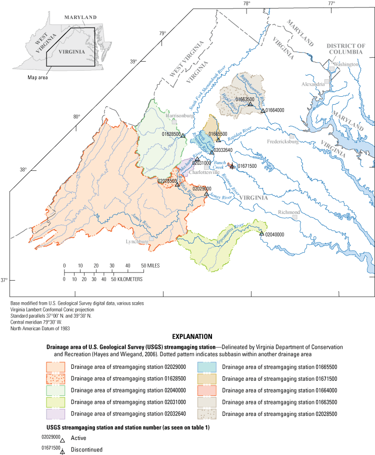
Map showing location of study sites. Sites are described in detail in table 1.
Table 1.
Descriptive statistics of study sites. Data from the USGS National Water Information System (U.S. Geological Survey, 2019).[ft3/s, cubic feet per second; mi2, square miles; VA, Virginia; S, south; N, north; F, fork]
| Site number (see fig. 1) | Station number | Station description | Approximate years of record | Mean daily value (ft3/s) | Minimum daily value (ft3/s) | Maximum daily value (ft3/s) | Range of daily values (ft3/s) | Median daily value (ft3/s) | Drainage area (mi2) | Decimal latitude (decimal degrees) | Decimal longitude (decimal degrees) | |
|---|---|---|---|---|---|---|---|---|---|---|---|---|
| 1 | 02029000 | James River at Scottsville, VA | 89 | 5,170.75 | 300.00 | 208,000.00 | 207,700.00 | 3,160.00 | 4,585 | 37.797365 | 78.491398 | |
| 2 | 01664000 | Rappahannock River at Remington, VA | 71 | 689.14 | 2.90 | 64,000.00 | 63,997.10 | 415.00 | 620 | 38.53068 | 77.813605 | |
| 3 | 01628500 | S F Shenandoah River Near Lynnwood, VA | 83 | 1,028.81 | 84.00 | 63,500.00 | 63,416.00 | 600.00 | 1,078 | 38.322628 | 78.754746 | |
| 4 | 02040000 | Appomattox River at Mattoax, VA | 88 | 693.51 | 2.60 | 34,300.00 | 34,297.40 | 376.00 | 725 | 37.421538 | 77.858888 | |
| 5 | 01665500 | Rapidan River near Ruckersville, VA | 71 | 154.37 | 0.45 | 29,400.00 | 29,399.55 | 96.00 | 115 | 38.280686 | 78.340007 | |
| 6 | 01663500 | Hazel River at Rixeyville, VA | 71 | 338.93 | 1.10 | 34,600.00 | 34,598.90 | 210.00 | 285 | 38.591789 | 77.964996 | |
| 7 | 02028500 | Rockfish River near Greenfield, VA | 71 | 141.25 | 0.07 | 28,800.00 | 28,799.93 | 85.00 | 95 | 37.869585 | 78.823354 | |
| 8 | 02031000 | Mechums River near White Hall, VA | 71 | 105.47 | 0.00 | 10,600.00 | 10,600.00 | 66.00 | 95 | 38.102636 | 78.592794 | |
| 9 | 02032640 | N F Rivanna River near Earlysville, VA | 20 | 125.19 | 0.28 | 11,000.00 | 10,999.72 | 64.00 | 108 | 38.163467 | 78.424732 | |
| 10 | 01671500 | Bunch Creek near Boswells Tavern, VA | 31 | 4.77 | 0.00 | 442.00 | 442.00 | 2.10 | 4 | 38.031806 | 78.191392 | |
Data Evaluation
Period-of-record daily-flow value streamflow data and period-of-record instantaneous value streamflow data beginning in 1990 were acquired for the 10 study sites from the USGS National Water Information System (NWIS) (U.S. Geological Survey, 2019). Histograms and continuous distributions of period-of-record daily-flow value streamflow data were prepared for the data collected at each site. Time series and bivariate trend analyses for each site were performed to identify any potential trends in data. An optimum (best fitting) probability density function determined by ranked Akaike Information Criterion (SAS Institute Inc., 2012), an estimator of prediction error describing the distribution of measured daily-flow values, was selected for each dataset from a comparison set of 12 computed candidate distributions spanning a range of potential distribution shapes specific to each study site (SAS Institute Inc., 2012) (fig. 2).
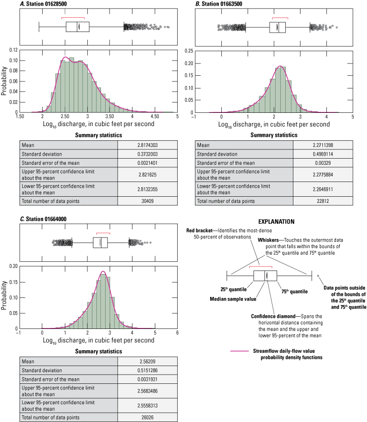
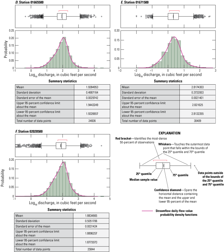
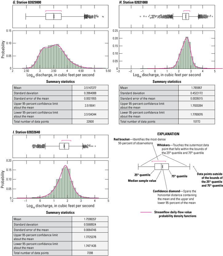
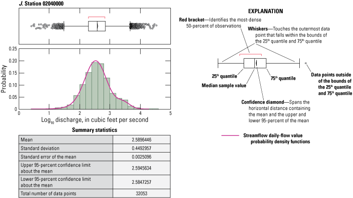
Graphs showing streamflow daily-flow value probability density functions for the 10 study sites. Each probability density function is the best-fitting function selected from a group of 12 computed basin specific candidate probability density functions.
Analysis and Tool Development
Hydrologic data were analyzed to develop tools to help determine streambed scour at bridge piers. Deterministic, probabilistic, and statistical modeling approaches were used to characterize and estimate hydrological outcomes of interest to VDOT, recognizing that each of these modeling approaches has unique strengths.
-
Deterministic modeling identifies and describes system elements (parts) and simulates cause-and-effect changes over time caused by links and interactions among identified elements of a system. System dynamics modeling, a type of deterministic modeling, allows identification and simulation of effects of endogenous (internally generated) feedback among model elements. This provides powerful opportunities to more fully identify and better understand causal links, interactions, reinforcing and compensating feedback mechanisms, and shifts in loop dominance (the most influential feedback loops in a system of causes and effects) that are part of the real-world, nonlinear systems being studied (Forrester, 1971).
-
Probabilistic modeling provides robust ways to understand likely outcomes of particular events within the context of previous events and conditions, often without the benefit of clear or complete knowledge of mechanisms, links, and delays associated with a particular combination of causes and effects (Hosmer and Lemeshow, 2000).
-
Statistical modeling provides numerous ways to sort through and manage distinctions among specific cause-and-effect signals and the separation of a signal from noise. Causation and distinctions among explanatory and response effects often may be successfully identified using well established and time-tested methods (Patterson and others, 2013; Sall and others, 2007; Yevjevich, 1967).
Each of these analytical approaches was used singly, and at times in combination with another analytical approach, to produce tools to determine and predict hydrological elements needed for estimating streambed scour rates over the design lifespans of highway bridges. Methods of analysis and the processes involved when developing eight tools are discussed in the remainder of this section of the report. Each tool is classified based on predominant modeling method used: (1) deterministic modeling, (2) probabilistic modeling, or (3) statistical modeling.
Deterministic Modeling Tools
Tool 1: A Generalized System Dynamics Model of Streamflow and Sediment Motion
Founded on the scientific method, system dynamics modeling provides a unique way to visualize and understand causal links, interactions, and feedback dynamics associated with complex multiorder nonlinear endogenous feedback systems. The method is particularly applicable to the dynamics of natural systems, which exhibit nonlinear feedback behaviors as consequences of system structure. Embedded causal loops often generate interconnected behavior patterns and shifts in loop dominance over time, internal to the system, that may be self-reinforcing or self-compensating.
Such feedback behaviors manifest themselves within the interconnected system created by causal links among components of streamflow, streambed particle shear stress, and streambed scour rate (fig. 3). Shear at the streambed, as influenced by the interplay of feedback between water-shear velocity and bed-sediment particle size, is one example. Increases in water velocity can scour streambed sediments, which then may decrease median streambed sediment size, accelerating rates of streambed sediment scour and resulting in potential increases in volumes of sediment removed from bridge piers. Conversely, decreases in water velocity can deposit streambed sediments, which then may increase median streambed sediment size, dampening rates of streambed sediment scour and resulting in potential decreases in volumes of sediment removed from bridge piers. Other changes from causal links within this system, such as increases in channel hydraulic radius or decreases in channel slope, may eventually regulate rates of streambed sediment scour or deposition. Any regulation or other adjustments, however, are dependent upon the characteristics of channel geomorphology and the overall hydrologic regime associated with the stream setting and bridge installation (fig. 3).
A common method of developing a system dynamics model begins with identifying one or more reference behavior modes that describe time-series responses associated with the question being addressed (Forrester, 1971; Richardson and Pugh, 1983). These are often illustrated using graphs of problem behavior-over-time. A causal-loop diagram is then created, mapping the links and interactions among the elements identified as associated with the question or problem. Reinforcing, compensating, and delayed effects and influences among elements are identified and noted as part of the causal-loop diagram. The graphs of reference behavior mode(s) together with causal-loop diagram(s) provide a qualitative description of the system of interest and an illustration of a proposed system structure that may be causing the behavior being addressed. State (stock) and rate (flow) variables often are mapped as a third step, to distinguish between stocks, in which information and physical elements often accumulate and are stored over intervals of time, and flows, which describe the movement of information and physical elements among the entities identified in the model. Once mapped, the stock and flow variables are populated with equations that describe the interactions and varying rates of change among them. When simulated, these interactions and varying rates of change often identify loops of cause-and-effect that may generate feedback effects and shifts in loop dominance over time. What emerges is a web of interacting causes and effects—a system that describes dynamic change-over-time that often is endogenous and creates its own behavior, which may be thought of as an articulation of a dynamic hypothesis of system interaction (Richardson and Pugh, 1983). Precisely this type of dynamic hypothesis, focused on questions specific to streambed scour, sediment removal, and sediment deposition is identified by the generalized system dynamics model of streamflow and sediment motion (fig. 4).
The generalized system dynamics model of streamflow and sediment motion facilitates detailed exploration of these interconnected effects. The model investigates hydrologic elements of these interactions using theoretical estimates of sediment motion, developed using Shields-curve relations as a proxy for empirical values (Maidment, 1993). Relations are described as multiorder discrete difference equations (table 2). A set of interactions in the model describes the interplay between water-shear velocity and bed-sediment particle size. As streamflow increases, the ratio of streamflow (Q) to critical streamflow (Q•) increases, causing bed-sediment scour rate to increase and net sediment removal from the streambed. If sediment particles at depth (beneath the bed-surface) are smaller than the bed-surface sediments that were previously in place, median bed sediment size decreases with sediment removal, and the specific weight of sediment decreases causing a reduction in the Q• threshold and an accelerating rate of streambed scour. Conversely, as streamflow decreases, the ratio of Q to Q• decreases, causing bed-sediment scour rate to decrease and net sediment addition to the streambed. If sediment particles at depth (beneath the bed-surface) are larger than the bed-surface sediments that were previously in place, median bed sediment size increases, and the specific weight of sediment increases causing an increase in the Q• threshold and a decelerating rate of streambed scour (fig. 5).
The reinforcing (positive) effects of increasing streambed scour associated with a stream-water velocity and bed-sediment feedback loop in which median sediment sizes decrease with depth will continue until regulated by a compensating (negative) counter affect. Possible compensating affects could be (1) an increase in bed sediment size with depth, (2) an increase in channel width resulting in a decrease in flow depth and net increase in channel roughness, or (3) a decrease of channel slope.
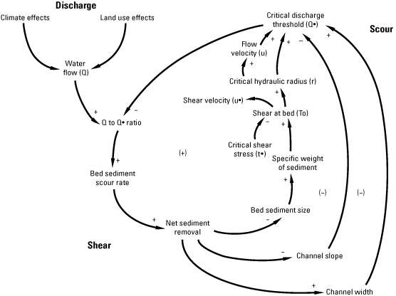
Diagram showing generalized streamflow and sediment motion causal loop diagram. A ‘+’ symbol indicates a positive (reinforcing) causal link. A ‘–’ symbol indicates a negative (compensating) causal link. A ‘(+)’ notation indicates a net-positive (reinforcing) loop of causal links. A ‘(–)’ notation indicates a net-negative (compensating) loop of causal links.
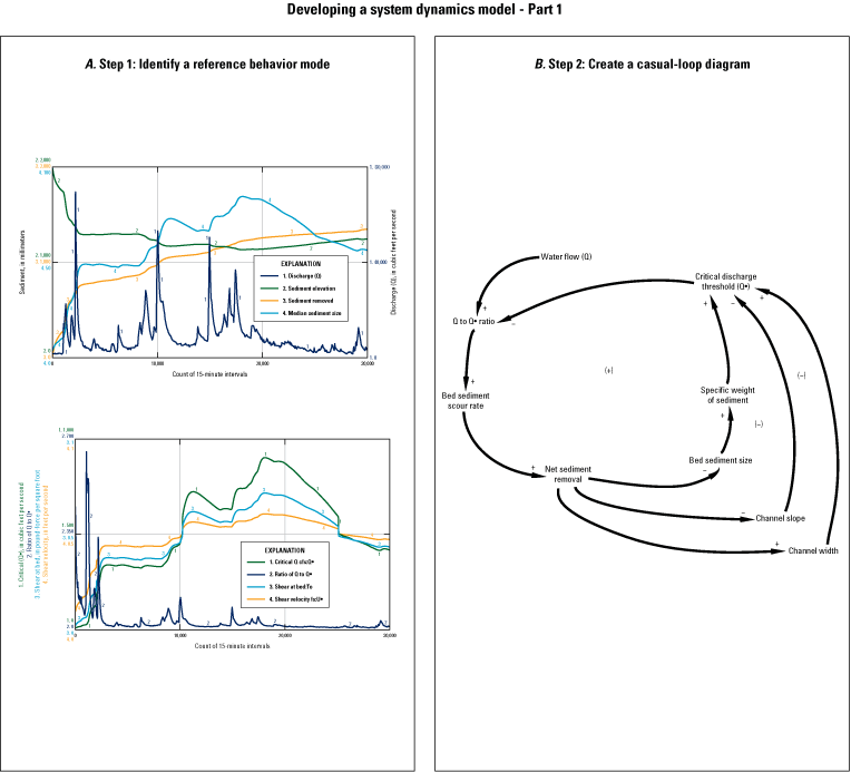
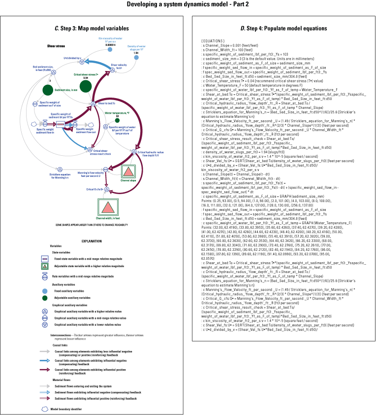
Steps in developing a system dynamics model. A, Step 1 involves using graphs to identify reference behavior over time. B, In step 2, a casual-loop diagram is created with major model elements. Minus signs (–) indicate negative (compensating) feedback. Plus signs (+) indicate positive (reinforcing) feedback. C, System dynamics model structural elements are identified in step 3. D, Step 4 populates discrete difference equations. ft3, cubic feet; ft2, square feet; s, second; mm, millimeter; lbf, pound-force; Ys, specific weight of sediment; Yf, specific weight of water; F, degrees Fahrenheit; R, hydraulic radius; U, flow velocity; n, Manning’s n; Q, streamflow in cubic feet per second; Q•, critical streamflow in cubic feet per second; Shear Vel fs:U•, bed shear velocity in feet per second; Bed sediment size in feet ft:d50, bed sediment particle mean diameter in feet.
Table 2.
Generalized streamflow and sediment motion discrete difference equations. Each line in the table documents one discrete difference equation.[t, time; dt, delta-time; ft, feet; mm, millimeter; s, second; lb., pounds; F, degrees Fahrenheit]
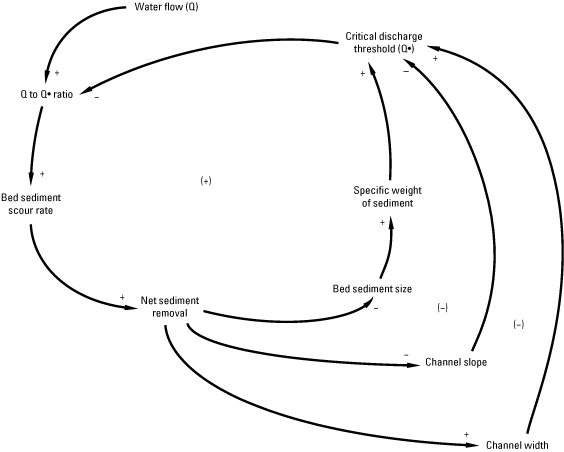
Diagram showing water velocity and bed sediment feedback loop. A ‘+’ symbol indicates a positive (reinforcing) causal link. A ‘–’ symbol indicates a negative (compensating) causal link. A ‘(+)’ notation indicates a net-positive (reinforcing) loop of causal links. A ‘(–)’ notation indicates a net-negative (compensating) loop of causal links.
Tool 2: Hydraulic Geometry At-a-Station Relations
Using methods pioneered by Leopold and others (1964), at-a-station hydraulic geometry was described for the James River at Scottsville, Virginia (station number 02029000). Knowledge of variation in hydraulic characteristics at a given cross section may be used to better understand and estimate likely changes in channel width, channel depth, water velocity, suspended-sediment load, river-bed slope, and channel roughness. Change-over-time in any of these characteristics may contribute to fluctuations in bed scour, with potential consequences for bridge-pier installations.
Streamflow field measurement statistics, including channel width, depth, and streamflow depth-averaged velocity measurements were accessed and retrieved from the USGS NWIS (U.S. Geological Survey, 2019). Measurements of channel width, channel depth, and channel depth-averaged velocity were combined with period-of-record streamflow data and plotted. Nonlinear regression was used to evaluate channel hydraulic geometry using the following relation, where streamflow hydraulic geometry is expressed as a function of water width, depth, and velocity:
Q is streamflow and w, d, and v are, respectively, water width, mean water depth, and mean water velocity, each of which may be represented as a function of streamflow with a, c, and k as intercept parameters and b, f, and m as slope parameters (Leopold and others, 1964).Tool 3: System Dynamics Model of Streambed Scour Incorporating Instantaneous Flows
A system dynamics model was developed using Monte-Carlo sampling of instantaneous streamflow measurements to augment and increase the precision of site-specific period-of-record mean daily-flow values (DV) potentially driving stream-power and streambed-scour estimates. Instantaneous streamflow values for each study site, collected and recorded in Virginia beginning in 1990 at 15- and 30-minute (min) intervals, were accessed and retrieved from the USGS NWIS (U.S. Geological Survey, 2019). Each instantaneous flow value was associated with its corresponding mean daily-flow value, the average of all instantaneous-flow values identified as occurring over the same daily interval. A set of frequency distributions of instantaneous values associated with each daily-flow value was then determined. Identifying the distribution of instantaneous values associated with each daily-flow value since 1990 provided a relation of likely instantaneous flows to all daily-flow values over the period-of-record at each test site. At each 15-min time step in the model a daily-flow value was presented and Monte-Carlo methods were used to select a likely associated instantaneous value (Maidment, 1993). The likely instantaneous values associated with each mean daily-flow value over the period-of-record identify variation in instantaneous flow not available from a mean daily-flow value alone, providing increased precision in flow estimation that may improve subsequent estimates of stream power and streambed scour associated with erosion of streambed sediments at bridge piers (fig. 6).
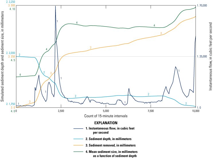
An example 104-day scour simulation illustrating 10,000 sampled 15-minute interval instantaneous-flow values driving change in millimeters of simulated sediment depth and change in sediment size in millimeters.
Probabilistic Modeling Tools
Tool 4: Probabilistic Sampling of Instantaneous Flows
Deterministic modeling was integrated with maximum likelihood logistic regression (MLLR) (Fawcett, 2006; Austin, 2014; Austin and Nelms, 2017) and Monte-Carlo sampling to create a probabilistic modeling tool that leverages the likelihood of instantaneous flows associated with daily-flow values (fig. 7). The process is initiated within the deterministic portion of the model, where a new daily-flow value is presented at each model iteration time-step. The daily-flow value presented is associated with all instantaneous-flow values likely to occur with the daily-flow value. A computed distribution of instantaneous values associated with the daily-flow value is identified and MLLR is used to compute the probabilities of occurrence of all associated instantaneous-flow values. Monte-Carlo sampling logic is then used to randomly select a likely instantaneous flow value from the MLLR distribution of probable choices. The deterministic portion of the model then determines whether to use the selected instantaneous flow value or the selected daily-flow value based on model logic that assigns an adjustable acceptable level of risk to the outcome. Model outcomes may be more, or less, risk-averse based on guidance from managers. The sequence of steps repeats with new information at each model time-step, resulting in a hydrological time-series that may be used in scour predictions. Each time-series is unique; a superset of unique time-series may be generated and compared to identify the most likely outcomes associated with many potentially different states of future flows (fig. 7).
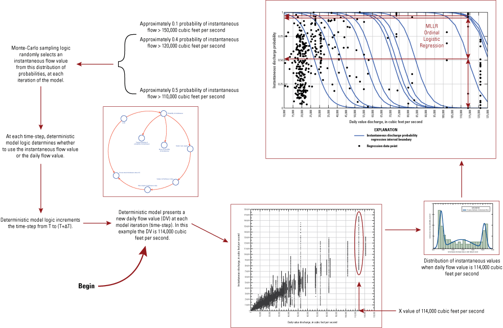
Probabilistic sampling of instantaneous flow. Deterministic, maximum likelihood logistic regression (MLLR), and Monte-Carlo methods are used to generate probable hydrology time series for modeling bridge pier scour. T, time, ΔT, change in time.
Tool 5: Instantaneous Flow Hydrologic Envelope Profiles
Instantaneous flow data were integrated with measured daily-flow value data to create instantaneous flow hydrologic envelope profiles for selected test sites. These were designed to enhance the precision of flow time-series for use in scour evaluations, providing easily accessible, conservative, and accurate estimates of water flux over short time steps. For selected sites, envelope profiles were prepared using Monte-Carlo sampling of instantaneous streamflow values, performed at each time step over the entire daily-flow value period-of-record. Each of these new records provided a unique period-of-record time series, incorporating the most likely instantaneous-flow values potentially associated with each measured daily-flow value. This sampling and instantaneous streamflow assignment process was repeated at least 30 times for each of the period-of-record daily-flow values associated with each test site. A unique integrated time series was generated after each repetition. Maximum and mean values associated with the repeated processes at each time step were then used to create two envelope curves for each test site—one describing likely mean flows associated with each daily time step and another describing likely maximum flows associated with each daily time step (fig. 8).
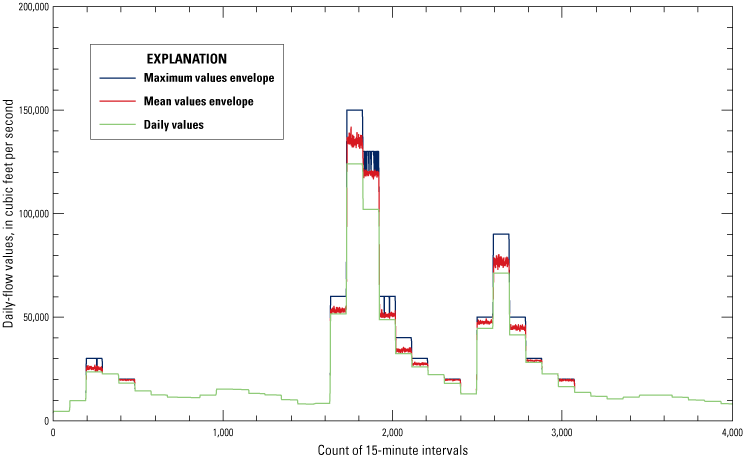
An illustration of Monte-Carlo identified period-of-record instantaneous value hydrologic envelope profiles. A 36.5-day subset of data generated for site 02029000, James River, Scottsville, Virginia, is shown illustrating the maximum values envelope curve (blue), mean values envelop curve (red), and corresponding daily-flow value streamflow data (green).
Tool 6: Sampled Instantaneous Flow Period-of-Record Time Series
To provide precise estimates of hydrologic flow over entire data time-series, which could be used to drive scour simulation models, sampled instantaneous flow period-of-record time series were prepared for selected test sites. Each prepared time-series dataset contained Monte-Carlo sampled 15-min interval instantaneous-flow values for the study site daily-flow value period-of record. This consisted of as many as 4 million sampled instantaneous-flow values per study site. Creation of each time-series dataset involved careful evaluation and preparation of instantaneous flow value probability density functions organized sequentially across a set of daily-flow value incremental size steps; figure 9 illustrates one set of these datasets, a series of probability density functions prepared for log10 daily-flow value size steps from 2.7 through 5.1. The sampling of instantaneous flows across the range of sequentially organized probability density functions provides a way to visualize and compare daily-flow values and estimated instantaneous-flow values at varying degrees of granularity, including daily-, weekly-, monthly-, seasonal-, and annual-time-step intervals (fig. 10).
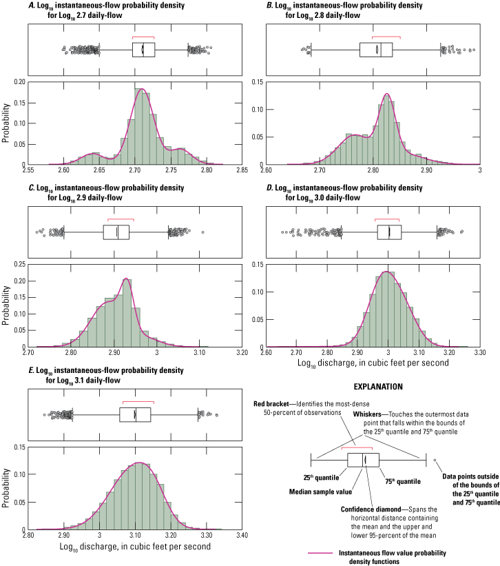
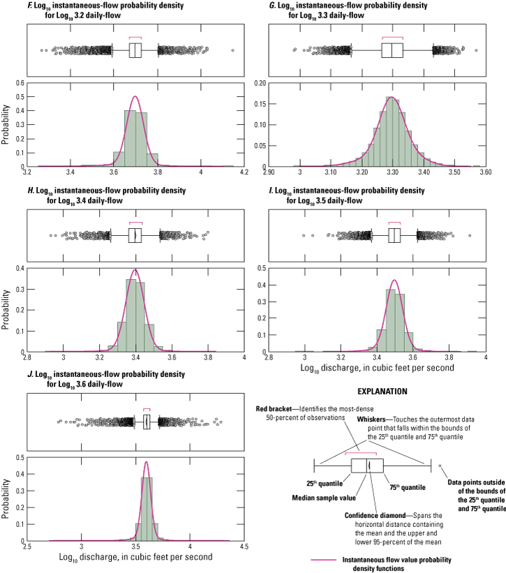
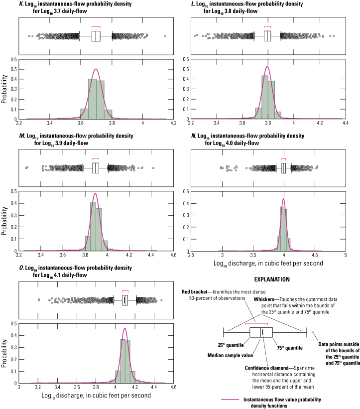
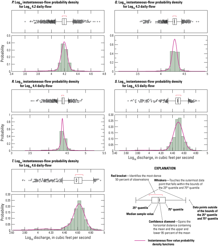
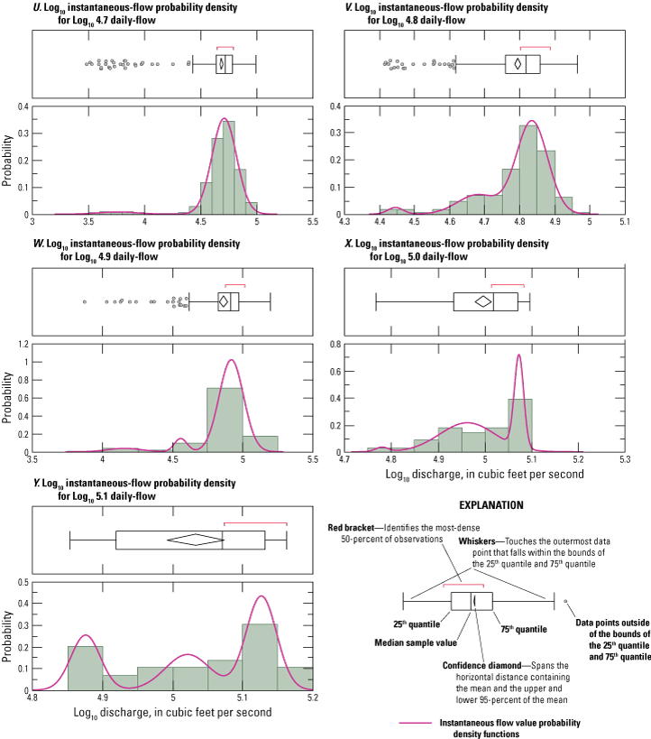
Graphs showing instantaneous flow value probability density functions organized by daily-flow value (DV) incremental size steps for site 02029000, James River, Scottsville, Virginia.
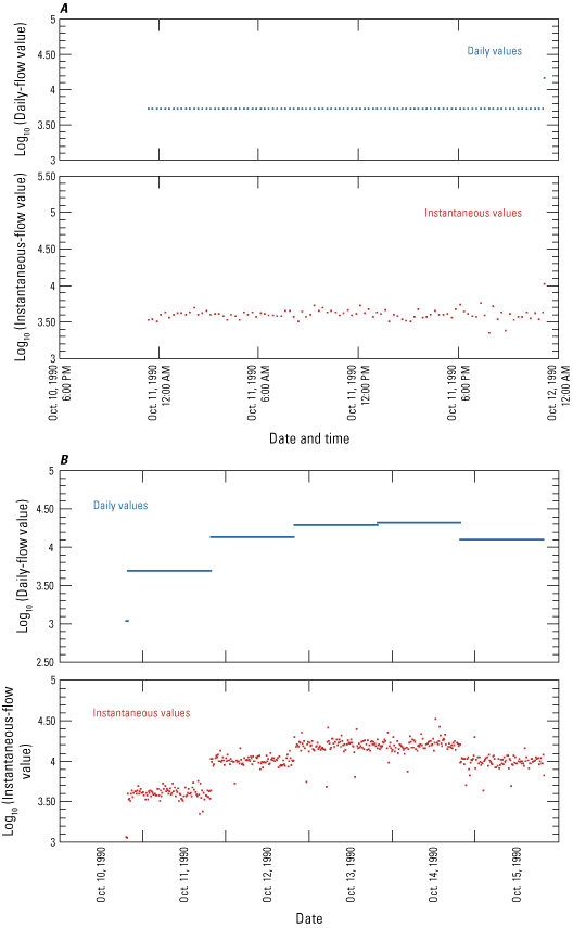
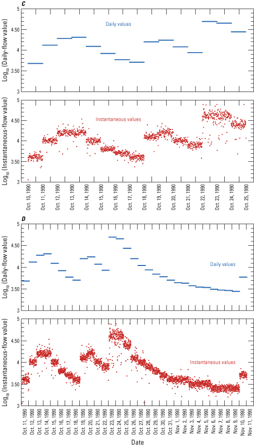
An illustration of potential visualization and comparison of daily-flow and instantaneous-flow values at differing time intervals: 1 day (A), 5 days (B), 15 days (C), and 31 days (D). Site 02029000, James River, Scottsville, Virginia.
Tool 7: Threshold of Flow and Probability of Time-Under-Load Interactive Calculator
Flow time-series data from the Nottoway River at Sebrell, Virginia (USGS station number 02047000), were used with elements of probability theory to develop a threshold of flow and probability of time-under-load interactive calculator that identifies the amount of time that a flow of a particular size is experienced over a selected bridge design lifespan. A desired bridge design lifespan and a flow interval of interest may be selected. Simulated bridge design lifespans range from 1 to 250 years, and flow intervals may be chosen, from minimum flow to maximum flow, as measured over the site’s period-of-record. With desired flow values selected, the interactive calculator displays the average chance (probability) of observing daily-flow values greater than or equal to flow within the identified range of flows. Probabilities are scaled from zero to one, with zero representing no probability of flow within the desired range, and one representing complete certainty of flow within the desired range. Probability results are further reported in day equivalents and year equivalents for the selected bridge design life span. For example, a selected design lifespan of 120 years for the Nottoway River at Sebrell, with a selected minimum flow threshold of 1,609 cubic feet per second and a selected maximum flow threshold of 60,000 cubic feet per second, yields a probability of observing daily-flow values greater than or equal to daily-flow values within the flow threshold interval range of 0.13, which is equivalent to 15.92 years or 5,810 days of streamflow within the identified range (fig. 11). Tool 7 facilitates interactive scenario analysis and feedback for management decision making.
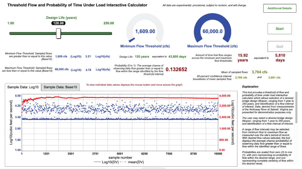
The threshold of flow probability and time-under-load interactive calculator. Base10, decimal numeral system; cfs, cubic feet per second; DV, daily-flow value; Log10, logarithm base 10 (See Appendix 1 for access to equations and example tools).
Statistical Modeling Tools
Tool 8: Flow Random Sampling Interactive Calculator
A flow random sampling interactive tool was developed to facilitate easy access to large datasets of randomly sampled flow data measurements from unique locations for purposes of computing and testing future models of bridge pier scour. The Nottoway River at Sebrell, Virginia (USGS station number 02047000), was identified as a useful site for compiling data and preparing methods to facilitate acquisition of large flow measurement datasets. Flow time-series data from the Nottoway River at Sebrell, Virginia, collected over the station’s period-of-record, were fitted to a Weibull distribution probability density function (Helsel and others, 2020). Probability and random sampling methods were used to create a flow random sampling interactive tool for the Nottoway River at Sebrell that provides real-time generation of, and on-demand access to, 36,500-datapoint random samples of streamflow data representing 100 years of mean daily-flow values. Using the tool allows acquisition of a new and unique 100-year set of daily-flow values with each interactive request of a new random sample. The interactive tool facilitates acquisition of uniquely sampled daily-flow values for experimentation, testing, and analysis of models that use large flow data sample sets (fig. 12).
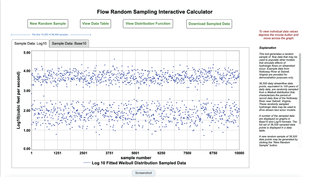
Flow random sampling interactive tool for Nottoway River at Sebrell, Virginia. Base10, decimal numeral system; Log10, logarithm base 10 (See Appendix 1 for access to equations and example tools).
Datasets
The datasets used to generate study analyses, calculations, and model output are published as a companion USGS data release (Austin, 2022). Datasets include
Results
Study deliverables are organized as tools that provide example analyses, data, and evaluation of daily and instantaneous streamflow, hydrologic elements, hydraulic geometry characteristics, streamflow probabilities, and simulation of probabilistic and deterministic streamflow duration. Equations are provided in appendix 1. Hydrologic properties associated with streambed scour are identified. Statistical methods demonstrate the use of sampled instantaneous streamflows, measured beginning in 1990, across the full period-of-record range of daily-flow values at a study site. The hydrologic statistics, statistical methods, and data-sampling techniques demonstrated in the tools may be used to assist in characterizing potential rates of streambed scour and estimating cumulative streambed scour at bridge pier locations over projected bridge design lifespans when combined with nonhydrologic elements provided by VDOT. Examples of nonhydrologic elements include bridge location and design specifications, attributes of cohesive soils associated with bridge piers, geotechnical attributes of bridge pier scour computations, and preferred specifications and methods for estimating soil scour.
Tools
Tool 1
A generalized system dynamics model of streamflow and sediment motion provides a generalized system dynamics model of streamflow and sediment motion that may be used to estimate hydrologic flow over time, likely thresholds of streambed sediment motion, and rates of streambed sediment scour. A key feature of the model is the structured design identifying a set of feedback loops that characterize reinforcing feedback effects of streambed sediment scour as influenced by water-velocity and bed sediment size.
Tool 2
The hydraulic geometry at-a-station relations tool illustrates at-a-station hydraulic geometry using methods pioneered by Leopold and others (1964). A key feature of this approach is the enhanced understanding of cross section variation in hydraulic characteristics provided by empirical relations that may be used to estimate likely changes in channel width, channel depth, water velocity, suspended-sediment load, river-bed slope, and channel roughness useful for evaluating bed scour at bridge piers.
Tool 3
A system dynamics model of streambed scour that incorporates instantaneous flows provides a method for testing the use of instantaneous streamflow measurements to drive stream-power and streambed scour estimates. The tool is structured to allow observation of outcomes from combinations of various ranges of input parameters. A unique feature of this approach is the ability to generate many estimates of future hydrologic flow scenarios, compile summary statistics, and identify likely flow scenarios.
Tool 4
Probabilistic sampling of instantaneous flows integrates deterministic modeling, MLLR, and Monte-Carlo sampling to identify probable hydrologic flows. The method leverages the likelihood of instantaneous flows associated with daily-flow values. The process is initiated by deterministic methods. A new daily-flow value is presented at each model iteration time-step. Instantaneous flows likely to occur with each daily-flow value are identified. MLLR computes instantaneous flow probabilities of occurrence. Monte-Carlo sampling logic randomly selects likely instantaneous-flow values, and deterministic model logic determines whether to employ an instantaneous or daily-flow value in hydrologic flow calculations based on an acceptable level of risk guided by management decisions. Unique features of this approach include integration of deterministic methods, Monte-Carlo sampling, and probabilistic methods; the option to identify scour multipliers associated with specific levels of streamflow; and the option to tailor model outcomes as more, or less, risk-averse using management input guidance.
Tool 5
Instantaneous flow hydrologic envelope profiles use measured instantaneous flow data integrated with measured daily-flow value data. Instantaneous flow hydrologic envelope profiles are designed to enhance precision of flow time-series estimates for use in scour evaluations and comparisons of mean daily-flow values, maximum daily-flow values, and instantaneous flows. They provide easily accessible, conservative, and accurate estimates of water flux over short time steps. A unique feature of these envelope profiles is that they are prepared using Monte-Carlo sampling of instantaneous streamflow values, providing estimates of instantaneous flows at each time step over the entire daily-flow value streamflow data period-of-record.
Tool 6
Sampled instantaneous flow period-of-record time series provide estimates of instantaneous hydrologic flow over entire daily-flow value data time-series, suitable for driving scour simulation models. Site-specific sampled instantaneous flow period-of-record time series were prepared. Each time-series dataset contains Monte-Carlo sampled 15-min interval instantaneous-flow values for the full study site daily-flow value period-of record, consisting of as many as 4 million sampled instantaneous-flow values per study site. Creation of each time-series dataset involved preparation and evaluation of instantaneous flow value probability density functions organized across a set of daily-flow value incremental size steps. The tool provides a means of visualizing and comparing daily-flow values and estimated instantaneous flows at varying degrees of granularity, including daily-, weekly-, monthly-, seasonal-, annual-, or other potentially useful intervals.
Tool 7
The threshold flow and probability of time-under-load interactive calculator allows selection of a desired bridge design lifespan, ranging from 1 to 250 years, and identification of a flow interval of interest. VDOT expressed interest in understanding and estimating the amount of time, over the design lifespan of a bridge, that the Nottoway River might be expected to achieve various stages of flow. Flow time-series data from the Nottoway River at Sebrell, Virginia, were used with elements of probability theory to develop the probability of time-under-load interactive calculator. A flow interval may be chosen, ranging from a minimum flow to a maximum flow as measured over the period-of-record of gage data associated with the Nottoway River at Sebrell, Virginia. As values are selected, the interactive calculator displays an average chance (probability) of observing daily-flow values greater than or equal to flow within the identified range of desired flows.
Tool 8
The flow random sampling interactive calculator provides a flow random sampling interactive tool, developed to facilitate easy access to large datasets of randomly sampled flow data measurements from unique locations for purposes of computing and testing future models of bridge pier scour. VDOT expressed interest in using stream flow data to drive models of bridge pier scour, and the Nottoway River at Sebrell, Virginia, was identified as a useful site for compiling data and preparing methods to facilitate acquisition of large flow measurement datasets. Flow time-series data collected over the station’s period-of-record, and fitted to a Weibull distribution probability density function, provide on-demand real-time generation of 36,500-datapoint random samples of streamflow data, allowing acquisition of unique 100-year sets of daily-flow value data with each interactive sample request.
Discussion
The analytical methods and tools described in this report demonstrate ways to improve the accuracy and utility of hydrologic flow estimates related to bridge pier scour. Each tool has strengths and weaknesses, and no single analytical approach can capture all aspects of hydrologic flow through natural river systems. As a matter of context, it is helpful to understand some of the details and distinctions among these empirical, theoretical, deterministic, and probabilistic methods of estimating hydrologic flows.
Empirical methods involve collection and analysis of field data that establish relations between variables or between variables and some aspect of a hydrologic process. The hydraulic geometry approach, as pioneered by Leopold and Maddock (1953) and used in Tool 2, is an excellent example of this type of empiricism in which relations described by power functions are used to analyze stream response to changing streamflow. Equations are flexible and the analytical techniques are sophisticated. Though problems may arise if generalizations from empirical results are based on an inadequate or overly restricted dataset, empirical approaches provide valuable insights into the unique relations of specific fluvial systems, and often may benefit further from the added, often systemic, understanding afforded by the underpinnings of a sound theoretical structure (Knighton, 1998).
Theoretical methods, which are further characterized below as deterministic and probabilistic, have at their core the formulation and testing of specific statements based on established principles, and often the construction and testing of simple or complex models (Knighton, 1998). Theoretical analyses often involve complex interactions among many variables. In certain instances, some degree of model abstraction or simplification is introduced and often framed by the model detail and granularity as sufficient to exploring and answering a previously identified set of specific questions or hypotheses. In some avenues of approach, such as system dynamics modeling, a structural representation of a system of interactions, built upon an identified reference behavior mode over time, is identified along with key feedback elements and endogenous characteristics to model the structure of the system that generates its own behavior over time. In these instances, and given a set of initial conditions, future outcomes based on a structured relation of interacting components may be revealed and tested. In system dynamics analysis this interactive, structured, endogenous relation of state variables and rate equations is described as a dynamic hypothesis. Methods specific to system dynamics modeling are used in Tools 1 and 3, and elements of theoretical analytical approaches are found in Tools 1, 3–6, and 7.
The deterministic method, one facet of theoretical analysis, is based on reasoned thought—the belief that physical laws control much of the behavior of natural systems—and that the behavior of natural systems can be predicted to a satisfactory level of accuracy, often associated with one or more previously identified questions once salient physical laws are recognized and understood. Deterministic equations often associated with hydrologic modeling include the continuity equation, flow-momentum equations, flow-resistance equations, and sediment-transport equations. Deterministic modeling often is used in a range of contexts including evaluations of channel initiation, drainage network development, meander development, prediction of channel topography, and prediction of particle entrainment (Knighton, 1998). Elements of deterministic analysis are found in Tools 1–7.
Probabilistic methods often are used when it is believed that the natural world, or at least the portion of it that is being investigated, is so complex that a meaningful deterministic explanation of the phenomena in question cannot be achieved. The same may be said of more generalized statistical analyses. Shreve (1975) discusses probabilistic and topologic approaches to drainage basin geology, writing that, “Geomorphic systems are descendants of antecedent states that are generally unknown, and they are invariably parts of larger systems from which they cannot be isolated…a probabilistic theory that takes account of [this] apparent randomness is evidently a necessity, because if our theories are to succeed, they must reflect the world as it is, not as we would like it to be.” Probabilistic analytical methods often are used when it is assumed that randomness exists in nature, that randomness is a fundamental property of natural systems, or that physical laws—perhaps combined with a lack of complete understanding—are not sufficient to identify or fully explain the system interactions driving a particular natural state or condition. Elements of probabilistic and statistical analysis are found in Tools 4–7 and 8.
When investigating and estimating hydrological flow, a combination of analytical approaches that meet specific analytical needs often offers the best chance of successfully characterizing a particular outcome of interest (Knighton, 1998). Most of the tools developed here combine elements of the analytical methods just described, and the manager or analyst should select the tool, or tools, that most appropriately address the question(s) at hand, within the scope of desired time and precision.
Conclusion
Analyses and hydrologic assessment tools developed in this study provide resources useful in the evaluation of streambed scour at bridge piers. Enhanced precision of flow estimates afforded by hydrological flow estimation methods that employ sampling of instantaneous flows across daily-flow periods-of-record appear particularly promising, as do the identification and evaluation of structural interactions and scour feedback affects using system dynamics models. Further evaluations of system structure, causal interactions, feedback affects, and shifts in loop dominance associated with stream power and flow resistance at the hydrological flow-streambed interface have the potential to reveal nonlinear reinforcing and compensating effects and elements of circular causality associated with bridge pier erosion, potentially yielding improved scour rate estimates over time. Future work building these types of system dynamics models linked to site-specific empirical hydrological flow, geotechnical, and channel materials data may significantly leverage understanding of scour dynamics at the bridge pier and streambed interface, yielding more complete insight into, and accurate estimates of, bridge pier scour rates.
More detailed studies of dynamic interactions among water, streambed surface, and bridge pier geometry and placement are needed to better characterize the often small, incremental changes in rates of streambed erosion and deposition that may deliver significant cumulative bridge pier erosive effects over long-term (100 years or more) bridge design lifespans. The dynamics of these interactions and any incremental changes in scour or deposition may include linked feedback effects and associated rates of change that need to be identified and studied yet are hard to perceive and measure over short- and medium-term time intervals. Any potentially reinforcing and structurally significant incremental effects spanning the longer time intervals that bridges and bridge piers are often designed to withstand need to be identified and carefully evaluated.
Summary
This report summarizes collaborative work by the U.S. Geological Survey (USGS) Virginia and West Virginia Water Science Center and the Virginia Department of Transportation (VDOT) investigating methods to evaluate rates of streambed scour in Virginia rivers and streams to improve cost effectiveness and safe design of highway bridge installations. VDOT and USGS entered into a cooperative agreement to provide estimates of hydrologic elements of bridge pier scour that may be combined with other geotechnical data in future scour evaluations. Investigations were limited to exploring hydrologic elements of scour estimates and preparing estimation tools using daily and instantaneous streamflow data.
Methods of evaluating scour that incorporate scour resistance estimates are now included in Federal Highway Administration guidance publications. Bridges with piers established in, or on, cohesive soil or erodible rock may now be designed so that scour resistance is considered within the bridge design lifespan. These new developments provided a rationale for initiating this study.
Several previous studies provided useful context, documenting the erosive properties of streambed scour. These include (1) a comprehensive set of investigations and methods for designing and evaluating bridges resistant to scour, (2) a new method developed to overcome limitations of applying bridge scour coarse-grained soil depth results to scour predictions associated with fine-grained soils, (3) studies comparing clear-water and live-bed scour depths associated with a single circular pile, and (4) an evaluation of 23 existing equations for local scour at bridge piers.
Ten sites in Virginia were selected for study, with drainage basin areas ranging from about 4 to 4,600 square miles in size, and stream discharge data collected over periods ranging from 20 to 89 years. Datasets were compiled, reviewed for errors, and used to prepare experimental analytical tools employing deterministic, probabilistic, and statistical analytical methods. System dynamics modeling of endogenous feedback—a deterministic modeling method—afforded unique opportunities to better understand system structure, causal links, interactions, reinforcing and compensating endogenous feedback, and shifts in loop dominance associated with erosive interactions of water and channel materials that create streambed scour. Probabilistic modeling provided useful insights into likely hydrologic flows, without the benefit of complete knowledge of causes and effects. Statistical modeling provided helpful distinctions among cause-and-effect signals, successfully identifying causation and distinctions among explanatory and response effects.
Eight experimental analytical tools were prepared. Three of the tools were developed using deterministic modeling methods, four tools were developed using probabilistic methods, and one tool was developed using other statistical methods. Distinctions among empirical, theoretical, deterministic, and probabilistic analytical methods were described. Datasets used for analyses were published as a USGS data release (Austin, 2022).
Selected References
Austin, S.H., 2014, Methods for estimating drought streamflow probabilities for Virginia streams: U.S. Geological Survey Scientific Investigations Report 2014–5145, 20 p., accessed October 2019 at https://doi.org/10.3133/sir20145145.
Austin, S.H., 2022, Virginia bridge scour pilot study streamflow data: U.S. Geological Survey data release, https://doi.org/10.5066/P957ABZN.
Austin, S.H., and Nelms, D.L., 2017, Modeling summer month hydrological drought probabilities in the United States using antecedent flow conditions: Journal of the American Water Resources Association, v. 53, no. 5, p. 1134–1146, accessed October 2019. https://doi.org/10.1111/1752-1688.12562.
Briaud, J.-L., Chen, H. -C., and Chang, K.-A., Oh, S.J., Chen, S., Wang, J., Li, Y., Kwak, K., Nartjaho, P., Gudaralli, R., Wei, W., Pergu, S., Cao, Y.W., and Ting, F., 2011, Summary report—The SRICOS-EFA method: College Station, Texas, Texas A&M University, 106 p., https://ceprofs.civil.tamu.edu/briaud/SRICOS-EFA/Summary%20of%20SRICOS-EFA%20Method.pdf.
Duggan, J., 2016, System dynamics modeling with R: Switzerland, Springer International Publishing, 176 p., accessed October 2019 at https://doi.org/10.1007/978-3-319-34043-2.
Falcone, J., 2011, GAGES-II—Geospatial attributes of gages for evaluating streamflow: U.S. Geological Survey web page, accessed December 2013 at http://water.usgs.gov/lookup/getspatial?gagesII_Sept2011.
Fawcett, T., 2006, An introduction to ROC analysis: Pattern Recognition Letters, v. 27, no. 8, p. 861–874, accessed October 2019 at https://doi.org/10.1016/j.patrec.2005.10.010.
Helsel, D.R., Hirsch, R.M., Ryberg, K.R., Archfield, S.A., and Gilroy, E.J., 2020, Statistical methods in water resources: U.S. Geological Survey Techniques and Methods, book 4, chap. A3, 458 p., https://doi.org/10.3133/tm4A3. [Super- sedes USGS Techniques of Water-Resources Investigations, book 4, chap. A3, version 1.1.]
Hosmer, D.W., and Lemeshow, S., 2000, Applied logistic regression: Hoboken, New Jersey, John Wiley and Sons, Inc., 383 p., accessed October 2019 at https://doi.org/10.1002/0471722146.
Leopold, L.B., and Maddock, T., Jr., 1953, The hydrologic geometry of stream channels and some physiographic implications: U.S. Geological Survey Professional Paper 252, 57 p., accessed September 2019 at https://doi.org/10.3133/pp252.
Leopold, L.B., Wolman, M.G., and Miller, J.P., 1964, Fluvial processes in geomorphology: Mineola, New York, Dover Publications, Inc., 522 p., accessed September 2019 at http://pubs.er.usgs.gov/publication/70185663.
Patterson, L.A., Lutz, B.D., and Doyle, M.W., 2013, Characterization of drought in the south Atlantic, United States: Journal of the American Water Resources Association, v. 49, no. 6, p. 1385–1397, accessed September 2019. https://doi.org/10.1111/jawr.12090.
Sheppard, D.M., and Miller, W., Jr., 2006, Live-bed local pier scour experiments: Journal of Hydraulic Engineering (New York, N.Y.), v. 132, no. 7, p. 635–642, accessed October 2019. https://doi.org/10.1061/(ASCE)0733-9429(2006)132:7(635).
Shreve, R.L., 1975, The probabilistic-topologic approach to drainage-basin geomorphology: Geology, v. 3, no. 9, p. 527–529, accessed October 2019. https://doi.org/10.1130/0091-7613(1975)3<527:TPATDG>2.0.CO;2.
U.S. Geological Survey, 2019, USGS water data for the nation: U.S. Geological Survey National Water Information System database, accessed June 2019 at https://doi.org/10.5066/F7P55KJN.
Yevjevich, V., 1967, An objective approach to definitions and investigations of continental hydrologic droughts—Hydrology paper 23: Fort Collins, Colorado, Colorado State University, 19 p., accessed August 2019 at https://doi.org/10.1016/0022-1694(69)90110-3.
Appendix 1. Equations
Tool 1: Equations for a Generalized System Dynamics Model of Streamflow and Sediment Motion
{INITIALIZATION EQUATIONS}
: s Channel_Slope = 0.001 {feet/feet}
: s Channel_Width_ft = 100 {feet}
: s sediment_depth = 2000 {initial condition is 2 meters of sediment (2000 mm) units are mm}
: s sediment_removed = 0 {Sediment removed by scour. Units are mm}
: s specific_weight_of_sediment_lbf_per_ft3:_Ys = 103
: c Q_climate_switch = 0 {0 = off, 1 = on}
: c Instantaneous_Q = 0 {Enter instantaneous Q values here.}
: c Q_adjustment = 0.01 {abritrarily multiply Q by this value}
: c discharge = Instantaneous_Q*Q_adjustment
: c Q_mult_from_climate = TIME
: f Q_cfs = IF Q_climate_switch = 1 THEN discharge*Q_mult_from_climate ELSE discharge
: c base_deposition_rate = 0.01 {Base deposition rate at Shields initiation of motion. Units are mm per time interval.}
: c sediment_size_mm = sediment_depth {3 is the default value. Units are in millimeters}
: c Bed_Sed_Size_in_feet_ft:d50 = sediment_size_mm/304.8 {feet}
: c Stricklers_equation_for_Manning's_n = (Bed_Sed_Size_in_feet_ft:d50^(1/6))/25.6 {Strickler's equation to estimate Manning's n}
: c Critical_shear_stress:T• = 0.04 {recommend critical shear stress (T•) value}
: c Water_Temperature_F = 50 {default temperature in degrees F}
: c specific_weight_of_water_lbf_per_ft3:_Yf_as_F_of_temp = Water_Temperature_F
: c Shear_at_bed:To = Critical_shear_stress:T•*(specific_weight_of_sediment_lbf_per_ft3:_Ys-specific_weight_of_water_lbf_per_ft3:_Yf_as_F_of_temp) * Bed_Sed_Size_in_feet_ft:d50
: c Critical_hydraulic_radius_'flow_depth'_ft:_R = Shear_at_bed:To / (specific_weight_of_water_lbf_per_ft3:_Yf_as_F_of_temp * Channel_Slope)
: c Manning's_Flow_Velocity_ft_per_second:_U = (1.49 / Stricklers_equation_for_Manning's_n) * (Critical_hydraulic_radius_'flow_depth'_ft:_R^(2/3) * Channel_Slope^(1/2))  {feet per second}
: c Critical_Q_cfs:Q• = Manning's_Flow_Velocity_ft_per_second:_U * Channel_Width_ft * Critical_hydraulic_radius_'flow_depth'_ft:_R {ft3 per second}
: c ratio_of_Q_to_Q• = Q_cfs /Critical_Q_cfs:Q• {ratio of actual discharge to critical discharge}
: c sed_dep_mult_from_Q = ratio_of_Q_to_Q• {units are dimensionless}
: f sed_dep_rate_mm_time = base_deposition_rate * sed_dep_mult_from_Q {units are mm per time interval}
: c base_scour_rate = 0.01 {Base scour rate at Shields initiation of motion. Units are mm per time interval.}
: c scour_rate_mult_from_Q = ratio_of_Q_to_Q• {Base scour rate multiplier as a function of Q. Units are dimensionless.}
: f sed_rem_rate_mm_time = base_scour_rate * scour_rate_mult_from_Q {units are mm per time interval}
: c specific_weight_of_sediment_as_F_of_size = sediment_size_mm
: f specific_weight_sed_flow_in = specific_weight_of_sediment_as_F_of_size
: f spec_weight_sed_flow_out = specific_weight_of_sediment_lbf_per_ft3:_Ys
: c Critical_shear_stress_result_check = Shear_at_bed:To/((specific_weight_of_sediment_lbf_per_ft3:_Ys-specific_weight_of_water_lbf_per_ft3:_Yf_as_F_of_temp)*Bed_Sed_Size_in_feet_ft:d50)
: c density_of_water_slugs_per_ft3 = 1.94 {slugs/ft3}
: c kin_viscosity_of_water_ft2_per_s:v = 1.4 * 10^-5  {square feet / second}
: c Shear_Vel_fs:U• = SQRT(Shear_at_bed:To/density_of_water_slugs_per_ft3) {feet  per second}
: c specific_gravity_of_sediment = 2.65
: c specific_weight_of_water_lbf_per_ft3:_Yf = 62.4 {lbf/ft3}
: c U•d_divided_by_v = (Shear_Vel_fs:U•*Bed_Sed_Size_in_feet_ft:d50)/kin_viscosity_of_water_ft2_per_s:v

{RUNTIME EQUATIONS}
: s Channel_Slope(t) = Channel_Slope(t - dt)
: s Channel_Width_ft(t) = Channel_Width_ft(t - dt)
: s sediment_depth(t) = sediment_depth(t - dt) + (sed_dep_rate_mm_time - sed_rem_rate_mm_time) * dt
: s sediment_removed(t) = sediment_removed(t - dt) + (sed_rem_rate_mm_time) * dt
: s specific_weight_of_sediment_lbf_per_ft3:_Ys(t) = specific_weight_of_sediment_lbf_per_ft3:_Ys(t - dt) + (specific_weight_sed_flow_in - spec_weight_sed_flow_out) * dt
: c discharge = Instantaneous_Q*Q_adjustment
: c Q_mult_from_climate = GRAPH(TIME)
Points: (0, 0.000), (421.052631579, 1.000), (842.105263158, 1.00321543408), (1263.15789474, 1.00321543408), (1684.21052632, 1.01607717042), (2105.26315789, 1.0192926045), (2526.31578947, 1.02893890675), (2947.36842105, 1.03536977492), (3368.42105263, 1.04501607717), (3789.47368421, 1.05466237942), (4210.52631579, 1.06752411576), (4631.57894737, 1.09324758842), (5052.63157895, 1.12540192926), (5473.68421053, 1.15434083601), (5894.73684211, 1.19935691318), (6315.78947368, 1.26045016077), (6736.84210526, 1.32797427653), (7157.89473684, 1.38585209003), (7578.94736842, 1.44051446945), (8000, 1.56270096463)
: f Q_cfs = IF Q_climate_switch = 1 THEN discharge*Q_mult_from_climate ELSE discharge
: c sediment_size_mm = GRAPH(sediment_depth {3 is the default value. Units are in millimeters})
Points: (1000, 128.0), (1200, 64.0), (1400, 32.0), (1600, 16.0), (1800, 8.0), (2000, 3.0), (2200, 2.5), (2400, 2.25), (2600, 2.0), (2800, 1.5), (3000, 1.0)
: c Bed_Sed_Size_in_feet_ft:d50 = sediment_size_mm/304.8 {feet}
: c Stricklers_equation_for_Manning's_n = (Bed_Sed_Size_in_feet_ft:d50^(1/6))/25.6 {Strickler's equation to estimate Manning's n}
: c specific_weight_of_water_lbf_per_ft3:_Yf_as_F_of_temp = GRAPH(Water_Temperature_F)
Points: (32.00, 62.4190), (33.80, 62.3953), (35.60, 62.4260), (37.40, 62.4270), (39.20, 62.4280), (41.00, 62.4270), (42.80, 62.4260), (44.60, 62.4230), (46.40, 62.4200), (48.20, 62.4160), (50.00, 62.4110), (51.80, 62.4050), (53.60, 62.3980), (55.40, 62.3910), (57.20, 62.3820), (59.00, 62.3730), (60.80, 62.3630), (62.60, 62.3530), (64.40, 62.3420), (66.20, 62.3300), (68.00, 62.3170), (69.80, 62.3040), (71.60, 62.2900), (73.40, 62.2760), (75.20, 62.2610), (77.00, 62.2450), (78.80, 62.2290), (80.60, 62.2120), (82.40, 62.1940), (84.20, 62.1760), (86.00, 62.1580), (87.80, 62.1390), (89.60, 62.1190), (91.40, 62.0990), (93.20, 62.0780), (95.00, 62.0570)
: c Shear_at_bed:To = Critical_shear_stress:T•*(specific_weight_of_sediment_lbf_per_ft3:_Ys-specific_weight_of_water_lbf_per_ft3:_Yf_as_F_of_temp) * Bed_Sed_Size_in_feet_ft:d50
: c Critical_hydraulic_radius_'flow_depth'_ft:_R = Shear_at_bed:To / (specific_weight_of_water_lbf_per_ft3:_Yf_as_F_of_temp * Channel_Slope)
: c Manning's_Flow_Velocity_ft_per_second:_U = (1.49 / Stricklers_equation_for_Manning's_n) * (Critical_hydraulic_radius_'flow_depth'_ft:_R^(2/3) * Channel_Slope^(1/2))  {feet per second}
: c Critical_Q_cfs:Q• = Manning's_Flow_Velocity_ft_per_second:_U * Channel_Width_ft * Critical_hydraulic_radius_'flow_depth'_ft:_R {ft3 per second}
: c ratio_of_Q_to_Q• = Q_cfs /Critical_Q_cfs:Q• {ratio of actual discharge to critical discharge}
: c sed_dep_mult_from_Q = GRAPH(ratio_of_Q_to_Q• {units are dimensionless})
Points: (0.900, 0.000), (1.010, 0.053), (1.120, 0.141), (1.230, 0.220), (1.340, 0.335), (1.450, 0.467), (1.560, 0.634), (1.670, 0.881), (1.780, 1.189), (1.890, 1.559), (2.000, 2.000)
: f sed_dep_rate_mm_time = base_deposition_rate * sed_dep_mult_from_Q {units are mm per time interval}
: c scour_rate_mult_from_Q = GRAPH(ratio_of_Q_to_Q• {Base scour rate multiplier as a function of Q. Units are dimensionless.})
Points: (1, 0), (300.9, 50), (600.8, 100), (900.7, 300), (1200.6, 500), (1500.5, 1500), (1800.4, 3000), (2100.3, 5000), (2400.2, 11000), (2700.1, 30000), (3000, 100000)
: f sed_rem_rate_mm_time = base_scour_rate * scour_rate_mult_from_Q {units are mm per time interval}
: c specific_weight_of_sediment_as_F_of_size = GRAPH(sediment_size_mm)
Points: (0.25, 93.00), (0.5, 94.00), (1.0, 98.00), (2.0, 101.00), (4.0, 103.00), (8.0, 108.00), (16.0, 111.00), (32.0, 121.00), (64.0, 127.00), (128.0, 130.00), (256.0, 137.00)
: f specific_weight_sed_flow_in = specific_weight_of_sediment_as_F_of_size
: f spec_weight_sed_flow_out = specific_weight_of_sediment_lbf_per_ft3:_Ys
: c Critical_shear_stress_result_check = Shear_at_bed:To/((specific_weight_of_sediment_lbf_per_ft3:_Ys-specific_weight_of_water_lbf_per_ft3:_Yf_as_F_of_temp)*Bed_Sed_Size_in_feet_ft:d50)
: c kin_viscosity_of_water_ft2_per_s:v = 1.4 * 10^-5  {square feet / second}
: c Shear_Vel_fs:U• = SQRT(Shear_at_bed:To/density_of_water_slugs_per_ft3) {feet  per second}
: c U•d_divided_by_v = (Shear_Vel_fs:U•*Bed_Sed_Size_in_feet_ft:d50)/kin_viscosity_of_water_ft2_per_s:v

{TIME SPECS}
STARTTIME=9000
STOPTIME=11000
DT=1
INTEGRATION=Runge-Kutta 4
RUNMODE=NORMAL
PAUSEINTERVAL=0
Tool 2: Equations for Hydrologic Geometry At-a-Station Relations
{INITIALIZATION EQUATIONS}
: c chan_discharge = TIME
: c Fitted_Model_Chan_Vel = 0.0370532505510006 * chan_discharge ^ 0.450785369474287
: c Fitted_Model_Chan_Width = 302.039444952286 * chan_discharge ^ 0.0704623388141807
: c Fitted_Model_Gage_height = 0.0900095294873019 * chan_discharge ^ 0.480456713312396

{RUNTIME EQUATIONS}
: c chan_discharge = GRAPH(TIME){A partial listing follows}
Points: (1.0, 5720), (2.0, 2557.92163543), (3.0, 1338.17035775), (4.0, 802.821124361), (5.0, 801.608177172), (6.0, 5970.86882453), (7.0, 37324.1908007), (8.0, 20122.0783646), (9.0, 5318.3032368), (10.0, 858.9335604772033.96252129),•••(580.0, 5831.78875639), (581.0, 3774.20783646), (582.0, 6016.59284497), (583.0, 2312.02725724), (584.0, 1396.06473595), (585.0, 2792.79386712), (586.0, 8141.73764906), (587.0, 8239.8637138), (588.0, 4840)

: c Fitted_Model_Chan_Vel = 0.0370532505510006 * chan_discharge ^ 0.450785369474287
: c Fitted_Model_Chan_Width = 302.039444952286 * chan_discharge ^ 0.0704623388141807
: c Fitted_Model_Gage_height = 0.0900095294873019 * chan_discharge ^ 0.480456713312396

{TIME SPECS}
STARTTIME=1
STOPTIME=588
DT=0.25
INTEGRATION=Runge-Kutta 2
RUNMODE=NORMAL
PAUSE INTERVAL=0
Tool 3: Equations for a System Dynamics Model of Streambed Scour Incorporating Instantaneous Flows
{INITIALIZATION EQUATIONS}
: s Channel_Slope = 0.006*4581^-0.2518 {feet/feet}
: s Channel_Width_ft = 12.964*4581^0.4294
: s sediment_deposited = 0 {no sediment initially}
: s sediment_depth = 2000 {initial condition is 2 meters of sediment (2000 mm) units are mm}
: s sediment_removed = 0 {Sediment removed by scour. Units are mm}
: s specific_weight_of_sediment_lbf_per_ft3:_Ys = 103
: c base_deposition_rate = 0.01 {Base deposition rate at Shields initiation of motion. Units are mm per time interval.}
: c Q_climate_switch = 1 {0 = discharge, 1 = climate change value,  2 = climate change graph}
: c Q_selection = 1 {1 =actual values, 0 = 128847 cfs}
: c Random_Subset_of_10K_Inst_Q_From_1990_to_2007_2029001 = TIME
: c discharge = IF Q_selection = 1 THEN Random_Subset_of_10K_Inst_Q_From_1990_to_2007_2029001 ELSE  120 {cfs}
: c Q_mult_from_climate_value = 1.1  {a multiplier greater than 1 to test more aggressive flows}
: c Q_mult_from_climate_graph = TIME
: f Q_cfs = IF Q_climate_switch = 1 THEN discharge*Q_mult_from_climate_value  ELSE  IF Q_climate_switch = 2 THEN Q_mult_from_climate_graph  ELSE discharge
: c sediment_choice = 1 {select a sediment multiplier}
: c A:_sed_size_per_sed_depth_mm = sediment_depth {3 is the default value. Units are in millimeters}
: c B:_alternative_sed_size_per_sed_depth_mm = sediment_depth
: c C:_sed_size_single_value = 3 {millimeters}
: c sediment_size_mm = IF sediment_choice = 1 THEN A:_sed_size_per_sed_depth_mm ELSE IF sediment_choice = 2 THEN B:_alternative_sed_size_per_sed_depth_mm ELSE IF sediment_choice = 3 THEN C:_sed_size_single_value ELSE A:_sed_size_per_sed_depth_mm
: c Bed_Sed_Size_in_feet_ft:d50 = sediment_size_mm/304.8 {feet}
: c Stricklers_equation_for_Manning's_n = (Bed_Sed_Size_in_feet_ft:d50^(1/6))/25.6
: c Critical_shear_stress:T• = 0.04 {recommend critical shear stress (T•) value}
: c Water_Temperature_F = 50 {default temperature in degrees F}
: c specific_weight_of_water_lbf_per_ft3:_Yf_as_F_of_temp = Water_Temperature_F
: c Shear_at_bed:To = Critical_shear_stress:T•*(specific_weight_of_sediment_lbf_per_ft3:_Ys-specific_weight_of_water_lbf_per_ft3:_Yf_as_F_of_temp) * Bed_Sed_Size_in_feet_ft:d50
: c Critical_hydraulic_radius_'flow_depth'_ft:_R = Shear_at_bed:To / (specific_weight_of_water_lbf_per_ft3:_Yf_as_F_of_temp * Channel_Slope)
: c Manning's_Flow_Velocity_ft_per_second:_U = (1.49 / Stricklers_equation_for_Manning's_n) * (Critical_hydraulic_radius_'flow_depth'_ft:_R^(2/3) * Channel_Slope^(1/2))  {feet per second}
: c Critical_Q_cfs:Q• = Manning's_Flow_Velocity_ft_per_second:_U * Channel_Width_ft * Critical_hydraulic_radius_'flow_depth'_ft:_R {ft3 per second}
: c ratio_of_Q_to_Q• = Q_cfs /Critical_Q_cfs:Q• {ratio of actual discharge to critical discharge}
: c sed_dep_mult_from_Q_to_Q• = ratio_of_Q_to_Q• {units are dimensionless}
: f sed_dep_rate_mm_time = SMTH1(base_deposition_rate * sed_dep_mult_from_Q_to_Q•, 100) {units are mm per time interval}
: c base_scour_rate = 0.01 {Base scour rate at Shields initiation of motion. Units are mm per time interval.}
: c scour_rate_mult_from_Q_to_Q• = ratio_of_Q_to_Q• {Base scour rate multiplier as a function of Q. Units are dimensionless.}
: f sed_rem_rate_mm_time = SMTH1(MAX((base_scour_rate * scour_rate_mult_from_Q_to_Q•), 0), 100) {units are mm per time interval}
: f sed_in = sed_dep_rate_mm_time
: c specific_weight_of_sediment_as_F_of_size = sediment_size_mm
: f specific_weight_sed_flow_in = specific_weight_of_sediment_as_F_of_size
: f spec_weight_sed_flow_out = specific_weight_of_sediment_lbf_per_ft3:_Ys
: c Critical_shear_stress_result_check = Shear_at_bed:To/((specific_weight_of_sediment_lbf_per_ft3:_Ys-specific_weight_of_water_lbf_per_ft3:_Yf_as_F_of_temp)*Bed_Sed_Size_in_feet_ft:d50)
: c density_of_water_slugs_per_ft3 = 1.94 {slugs/ft3}
: c kin_viscosity_of_water_ft2_per_s:v = 1.4 * 10^-5  {square feet / second}
: c Shear_Vel_fs:U• = SQRT(Shear_at_bed:To/density_of_water_slugs_per_ft3) {feet  per second}
: c specific_gravity_of_sediment = 2.65
: c specific_weight_of_water_lbf_per_ft3:_Yf = 62.4 {lbf/ft3}
: c U•d_divided_by_v = (Shear_Vel_fs:U•*Bed_Sed_Size_in_feet_ft:d50)/kin_viscosity_of_water_ft2_per_s:v

{RUNTIME EQUATIONS}
: s Channel_Slope(t) = Channel_Slope(t - dt)
: s Channel_Width_ft(t) = Channel_Width_ft(t - dt)
: s sediment_deposited(t) = sediment_deposited(t - dt) + (sed_in) * dt
: s sediment_depth(t) = sediment_depth(t - dt) + (sed_dep_rate_mm_time - sed_rem_rate_mm_time) * dt
: s sediment_removed(t) = sediment_removed(t - dt) + (sed_rem_rate_mm_time) * dt
: s specific_weight_of_sediment_lbf_per_ft3:_Ys(t) = specific_weight_of_sediment_lbf_per_ft3:_Ys(t - dt) + (specific_weight_sed_flow_in - spec_weight_sed_flow_out) * dt
: c Random_Subset_of_10K_Inst_Q_From_1990_to_2007 = GRAPH(TIME) {partial listing follows}
Points: (53, 1080.0), (183, 1030.0), (192, 1010.0), (237, 1260.0), (280, 949.0), (403, 990.0), (413, 1150.0), (480, 1020.0), (510, 960.0), (570, 1280.0), ••• (801, 1120.0), (815, 1010.0), (879, 870.0), (900, 870.0)
: c discharge = IF Q_selection = 1 THEN Random_Subset_of_10K_Inst_Q_From_1990_to_2007_2029001 ELSE  120 {cfs}
: c Q_mult_from_climate_graph = GRAPH(TIME)
Points: (0, 0.000), (421.052631579, 1.000), (842.105263158, 1.00321543408), (1263.15789474, 1.00321543408), (1684.21052632, 1.01607717042), (2105.26315789, 1.0192926045), (2526.31578947, 1.02893890675), (2947.36842105, 1.03536977492), (3368.42105263, 1.04501607717), (3789.47368421, 1.05466237942), (4210.52631579, 1.06752411576), (4631.57894737, 1.09324758842), (5052.63157895, 1.12540192926), (5473.68421053, 1.15434083601), (5894.73684211, 1.19935691318), (6315.78947368, 1.26045016077), (6736.84210526, 1.32797427653), (7157.89473684, 1.38585209003), (7578.94736842, 1.44051446945), (8000, 1.56270096463)
: f Q_cfs = IF Q_climate_switch = 1 THEN discharge*Q_mult_from_climate_value  ELSE  IF Q_climate_switch = 2 THEN Q_mult_from_climate_graph  ELSE discharge
: c A:_sed_size_per_sed_depth_mm = GRAPH(sediment_depth {3 is the default value. Units are in millimeters})
Points: (1000, 128.0), (1200, 64.0), (1400, 32.0), (1600, 16.0), (1800, 8.0), (2000, 3.0), (2200, 3.0), (2400, 3.0), (2600, 3.0), (2800, 3.0), (3000, 3.0)
: c B:_alternative_sed_size_per_sed_depth_mm = GRAPH(sediment_depth)
Points: (1000, 128), (1200, 64), (1400, 32), (1600, 16), (1800, 8), (2000, 3), (2200, 3), (2400, 3), (2600, 3), (2800, 3), (3000, 3)
: c sediment_size_mm = IF sediment_choice = 1 THEN A:_sed_size_per_sed_depth_mm ELSE IF sediment_choice = 2 THEN B:_alternative_sed_size_per_sed_depth_mm ELSE IF sediment_choice = 3 THEN C:_sed_size_single_value ELSE A:_sed_size_per_sed_depth_mm
: c Bed_Sed_Size_in_feet_ft:d50 = sediment_size_mm/304.8 {feet}
: c Stricklers_equation_for_Manning's_n = (Bed_Sed_Size_in_feet_ft:d50^(1/6))/25.6 {Strickler's equation to estimate Manning's n}
: c specific_weight_of_water_lbf_per_ft3:_Yf_as_F_of_temp = GRAPH(Water_Temperature_F)
Points: (32.00, 62.4190), (33.80, 62.3953), (35.60, 62.4260), (37.40, 62.4270), (39.20, 62.4280), (41.00, 62.4270), (42.80, 62.4260), (44.60, 62.4230), (46.40, 62.4200), (48.20, 62.4160), (50.00, 62.4110), (51.80, 62.4050), (53.60, 62.3980), (55.40, 62.3910), (57.20, 62.3820), (59.00, 62.3730), (60.80, 62.3630), (62.60, 62.3530), (64.40, 62.3420), (66.20, 62.3300), (68.00, 62.3170), (69.80, 62.3040), (71.60, 62.2900), (73.40, 62.2760), (75.20, 62.2610), (77.00, 62.2450), (78.80, 62.2290), (80.60, 62.2120), (82.40, 62.1940), (84.20, 62.1760), (86.00, 62.1580), (87.80, 62.1390), (89.60, 62.1190), (91.40, 62.0990), (93.20, 62.0780), (95.00, 62.0570)
: c Shear_at_bed:To = Critical_shear_stress:T•*(specific_weight_of_sediment_lbf_per_ft3:_Ys-specific_weight_of_water_lbf_per_ft3:_Yf_as_F_of_temp) * Bed_Sed_Size_in_feet_ft:d50
: c Critical_hydraulic_radius_'flow_depth'_ft:_R = Shear_at_bed:To / (specific_weight_of_water_lbf_per_ft3:_Yf_as_F_of_temp * Channel_Slope)
: c Manning's_Flow_Velocity_ft_per_second:_U = (1.49 / Stricklers_equation_for_Manning's_n) * (Critical_hydraulic_radius_'flow_depth'_ft:_R^(2/3) * Channel_Slope^(1/2))  {feet per second}
: c Critical_Q_cfs:Q• = Manning's_Flow_Velocity_ft_per_second:_U * Channel_Width_ft * Critical_hydraulic_radius_'flow_depth'_ft:_R {ft3 per second}
: c ratio_of_Q_to_Q• = Q_cfs /Critical_Q_cfs:Q• {ratio of actual discharge to critical discharge}
: c sed_dep_mult_from_Q_to_Q• = GRAPH(ratio_of_Q_to_Q• {units are dimensionless})
Points: (0.900, 0.000), (1.010, 0.032), (1.120, 0.076), (1.230, 0.151), (1.340, 0.270), (1.450, 0.378), (1.560, 0.551), (1.670, 0.757), (1.780, 1.059), (1.890, 1.503), (2.000, 2.000)
: f sed_dep_rate_mm_time = SMTH1(base_deposition_rate * sed_dep_mult_from_Q_to_Q•, 100) {units are mm per time interval}
: c scour_rate_mult_from_Q_to_Q• = GRAPH(ratio_of_Q_to_Q• {Base scour rate multiplier as a function of Q. Units are dimensionless.})
Points: (1, 0), (300.9, 50), (600.8, 100), (900.7, 300), (1200.6, 500), (1500.5, 1500), (1800.4, 3000), (2100.3, 5000), (2400.2, 11000), (2700.1, 30000), (3000, 100000)
: f sed_rem_rate_mm_time = SMTH1(MAX((base_scour_rate * scour_rate_mult_from_Q_to_Q•), 0), 100) {units are mm per time interval}
: f sed_in = sed_dep_rate_mm_time
: c specific_weight_of_sediment_as_F_of_size = GRAPH(sediment_size_mm)
Points: (0.25, 93.00), (0.5, 94.00), (1.0, 98.00), (2.0, 101.00), (4.0, 103.00), (8.0, 108.00), (16.0, 111.00), (32.0, 121.00), (64.0, 127.00), (128.0, 130.00), (256.0, 137.00)
: f specific_weight_sed_flow_in = specific_weight_of_sediment_as_F_of_size
: f spec_weight_sed_flow_out = specific_weight_of_sediment_lbf_per_ft3:_Ys
: c Critical_shear_stress_result_check = Shear_at_bed:To/((specific_weight_of_sediment_lbf_per_ft3:_Ys-specific_weight_of_water_lbf_per_ft3:_Yf_as_F_of_temp)*Bed_Sed_Size_in_feet_ft:d50)
: c kin_viscosity_of_water_ft2_per_s:v = 1.4 * 10^-5  {square feet / second}
: c Shear_Vel_fs:U• = SQRT(Shear_at_bed:To/density_of_water_slugs_per_ft3) {feet  per second}
: c U•d_divided_by_v = (Shear_Vel_fs:U•*Bed_Sed_Size_in_feet_ft:d50)/kin_viscosity_of_water_ft2_per_s:v

{TIME SPECS}
STARTTIME=0
STOPTIME=10000
DT=1
INTEGRATION=Runge-Kutta 4
RUNMODE=NORMAL
PAUSEINTERVAL=0
Tool 4: Equations for Probabilistic Sampling of Instantaneous Flows
{INITIALIZATION EQUATIONS}
: s BKF_storm_interval_timer = 0
: s water_standing_on_land_surface = 0
: S bed_elevation_mm = 0 {millimeter}
: S cumulative_scour_mm = 0 {millimeters}
: f time_in = (TIME+RANDOM(1,300))/(TIME+0.000001)
: c total_inches_rainfall_in_24_hours_BKF = RANDOM(0.1,4,0.2) {inches}
: c base_deposition_rate = 0.01 {millimeters per day}
: c Q_selection = 1 {1 =inst values 0 = daily values}
: c "10K_Instantaneous_Values_02029000" = TIME
: c "10K_Daily_Values_02029000" = TIME
: c discharge = IF Q_selection = 1 THEN "10K_Instantaneous_Values_02029000" ELSE  "10K_Daily_Values_02029000"
: f Q_cfs = discharge
: c deposition_mult_from_Q = Q_cfs
: f deposition_rate_mm_per_day = base_deposition_rate * deposition_mult_from_Q
: c SCS_type_II_rainfall_distribution = BKF_storm_interval_timer
: f rainfall_in_acre_inches_per_hour = SCS_type_II_rainfall_distribution*total_inches_rainfall_in_24_hours_BKF
: c base_scour_rate = 0.01 {millimeters per day}
: c scour_mult_from_Q = Q_cfs
: c scour_mult_from_depth = bed_elevation_mm {millimeters}
: f scour_rate_mm_per_day = base_scour_rate * scour_mult_from_Q * scour_mult_from_depth {millimeters per day}
: c start_BKF_rainstorms? = 1 {1= yes 0=no}
: f time_out = IF(BKF_storm_interval_timer >200) THEN BKF_storm_interval_timer/DT*start_BKF_rainstorms? ELSE 0   {13,020 hours is approximately equal to 1.5 years, the average interval of Bankfull storm events}
: c initial_bed_elevation = 0
: c velocity_from_discharge = Q_cfs
: c shear_stress_from_velocity = velocity_from_discharge
: c scour_rate_from_shear_stress = shear_stress_from_velocity {shear stress is in (N/m3) and scour rate is in (mm/hour)}

 RUNTIME EQUATIONS}
: s BKF_storm_interval_timer(t) = BKF_storm_interval_timer(t - dt) + (time_in - time_out) * dt
: s water_standing_on_land_surface(t) = water_standing_on_land_surface(t - dt) + (rainfall_in_acre_inches_per_hour) * dt
: S bed_elevation_mm(t) = bed_elevation_mm(t - dt) + (deposition_rate_mm_per_day - scour_rate_mm_per_day) * dt
: S cumulative_scour_mm(t) = cumulative_scour_mm(t - dt) + (scour_rate_mm_per_day) * dt
: f time_in = (TIME+RANDOM(1,300))/(TIME+0.000001)
: c total_inches_rainfall_in_24_hours_BKF = RANDOM(0.1,4,0.2) {inches}

: c "10K_Instantaneous_Values_02029000" = GRAPH(TIME) {A partial listing}
Points: (1, 1500.000), (2, 1510.000), (3, 1510.000), (4, 1510.000), •••
(9995, 44300.000), (9996, 44300.000), (9997, 44400.000), (9998, 44400.000), (9999, 44600.000), (10000, 44700.000)

: c "10K_Daily_Values_02029000" = GRAPH(TIME) {A partial listing}
Points: (1, 1165.46875), (2, 1165.46875), (3, 1165.46875), (4, 1165.46875), (5, 1165.46875), ••• (9998, 44231.250), (9999, 44231.250), (10000, 44231.250)

: c discharge = IF Q_selection = 1 THEN "10K_Instantaneous_Values_02029000" ELSE  "10K_Daily_Values_02029000"
: f Q_cfs = discharge
: c deposition_mult_from_Q = GRAPH(Q_cfs)
Points: (0.0, 0.59807073955), (2.04081632653, 0.16077170418), (4.08163265306, 0.064308681672), (6.12244897959, 0.0385852090032), (8.16326530612, 0.032154340836), (10.2040816327, 0.0128617363344), (12.2448979592, 0.000), (14.2857142857, 0.000), (16.3265306122, 0.000), (18.3673469388, 0.000), (20.4081632653, 0.000), (22.4489795918, 0.000), (24.4897959184, 0.000), (26.5306122449, 0.000), (28.5714285714, 0.000), (30.612244898, 0.000), (32.6530612245, 0.000), (34.693877551, 0.000), (36.7346938776, 0.000), (38.7755102041, 0.000), (40.8163265306, 0.000), (42.8571428571, 0.000), (44.8979591837, 0.000), (46.9387755102, 0.000), (48.9795918367, 0.000), (51.0204081633, 0.000), (53.0612244898, 0.000), (55.1020408163, 0.000), (57.1428571429, 0.000), (59.1836734694, 0.000), (61.2244897959, 0.000), (63.2653061224, 0.000), (65.306122449, 0.000), (67.3469387755, 0.000), (69.387755102, 0.000), (71.4285714286, 0.000), (73.4693877551, 0.000), (75.5102040816, 0.000), (77.5510204082, 0.000), (79.5918367347, 0.000), (81.6326530612, 0.000), (83.6734693878, 0.000), (85.7142857143, 0.000), (87.7551020408, 0.000), (89.7959183673, 0.000), (91.8367346939, 0.000), (93.8775510204, 0.000), (95.9183673469, 0.000), (97.9591836735, 0.000), (100.0, 0.000)

: f deposition_rate_mm_per_day = base_deposition_rate * deposition_mult_from_Q

: c SCS_type_II_rainfall_distribution = GRAPH(BKF_storm_interval_timer)
Points: (0.00, 0.0000), (1.00, 0.0100), (2.00, 0.0150), (3.00, 0.0150), (4.00, 0.0200), (5.00, 0.0200), (6.00, 0.0250), (7.00, 0.0300), (8.00, 0.0350), (9.00, 0.0500), (10.00, 0.4200), (11.00, 0.1180), (12.00, 0.0470), (13.00, 0.0320), (14.00, 0.0280), (15.00, 0.0210), (16.00, 0.0200), (17.00, 0.0170), (18.00, 0.0170), (19.00, 0.0130), (20.00, 0.0110), (21.00, 0.0025), (22.00, 0.0000), (23.00, 0.0000), (24.00, 0.0000)

: f rainfall_in_acre_inches_per_hour = SCS_type_II_rainfall_distribution*total_inches_rainfall_in_24_hours_BKF

: c scour_mult_from_Q = GRAPH(Q_cfs)
Points: (103, 0.00), (3092.7, 0.00), (6082.4, 0.096463022508), (9072.1, 0.192926045016), (12061.8, 0.353697749196), (15051.5, 0.578778135048), (18041.2, 1.31832797428), (21030.9, 2.73311897106), (24020.6, 4.34083601286), (27010.3, 6.59163987138), (30000, 10.00)

: c scour_mult_from_depth = GRAPH(bed_elevation_mm {millimeters})
Points: (-10.00, 1.000), (-9.00, 1.16720257235), (-8.00, 1.34726688103), (-7.00, 1.61736334405), (-6.00, 1.87459807074), (-5.00, 2.08038585209), (-4.00, 2.08681672026), (-3.00, 1.89389067524), (-2.00, 1.55948553055), (-1.00, 1.22508038585), (0.00, 1.000)

: f scour_rate_mm_per_day = base_scour_rate * scour_mult_from_Q * scour_mult_from_depth {millimeters per day}

: f time_out = IF(BKF_storm_interval_timer >200) THEN BKF_storm_interval_timer/DT*start_BKF_rainstorms? ELSE 0   {13,020 hours is approximately equal to 1.5 years, the average interval of Bankfull storm events}

: c velocity_from_discharge = Q_cfs
: c shear_stress_from_velocity = velocity_from_discharge
: c scour_rate_from_shear_stress = GRAPH(shear_stress_from_velocity {shear stress is in (N/m3) and scour rate is in (mm/hour)})
Points: (0.0, 0.00), (100.0, 10.0964630225), (200.0, 13.5048231511), (300.0, 15.6270096463), (400.0, 16.00)

{TIME SPECS}
STARTTIME=1
STOPTIME=10000
DT=0.25
INTEGRATION=Runge-Kutta 2
RUNMODE=NORMAL
PAUSEINTERVAL=0
Tool 5: Equations for Instantaneous Flow Hydrologic Envelope Profiles
{INITIALIZATION EQUATIONS}
: c daily_values = TIME
: c "daily_values_+_inst" = TIME
: c maximum_values = TIME
: c mean_values = TIME
: c minute_intervals = TIME
: c Instantaneous_Monte_Carlo_Selection_Station_02029000 = TIME
: c "Inst_(cfs)" = 10^Instantaneous_Monte_Carlo_Selection_Station_02029000
: f Inst_in = "Inst_(cfs)"
: l Inst_conveyor = Inst_in
    TRANSIT TIME = averaging_time_in_15_minute_intervals
: f Inst_out = CONVEYOR OUTFLOW
: c "ROUNDED_Log10(DV)_Station_02029000" = TIME
: c DV = 10^"ROUNDED_Log10(DV)_Station_02029000"
: c "mean_flow_(cfs)" =  IF "mean_flow_averaging_time_(days)"-TIME > 0 THEN 0 ELSE MEAN(Inst_conveyor)

{RUNTIME EQUATIONS}
: c daily_values = GRAPH(TIME) {A partial listing follows}
Points: (1, 3790), (2, 3790), (3, 3907.0396582), (4, 4407.4079038), (5, 4450), (6, 4450), (7, 4450), (8, 4450), (9, 4450), (10, 4450), •••  (3198, 2194397), (3199, 2194398), (3200, 2194399), (3201, 2194400)

{TIME SPECS}
STARTTIME=1
STOPTIME=3201
DT=0.25
INTEGRATION=Runge-Kutta 2
RUNMODE=NORMAL
PAUSEINTERVAL=0
Tool 6: Equations for Sampled Instantaneous Flow Period-of-Record Time Series
{INITIALIZATION EQUATIONS}
: c "mean_flow_averaging_time_(days)" = 1 {day}
: c "15_minute_intervals_per_day" = 96 {15-minute intervals per day}
: c averaging_time_in_15_minute_intervals = "mean_flow_averaging_time_(days)"*"15_minute_intervals_per_day" {Inst value time units for average}
: c Instantaneous_Monte_Carlo_Selection_Station_02029000 = TIME
: c "Inst_(cfs)" = 10^Instantaneous_Monte_Carlo_Selection_Station_02029000
: f Inst_in = "Inst_(cfs)"
: l Inst_conveyor = Inst_in
    TRANSIT TIME = averaging_time_in_15_minute_intervals
: f Inst_out = CONVEYOR OUTFLOW
: c "ROUNDED_Log10(DV)_Station_02029000" = TIME
: c DV = 10^"ROUNDED_Log10(DV)_Station_02029000"
: c "mean_flow_(cfs)" =  IF "mean_flow_averaging_time_(days)"-TIME > 0 THEN 0 ELSE MEAN(Inst_conveyor)

{RUNTIME EQUATIONS}
: l Inst_conveyor(t) = Inst_conveyor(t - dt) + (Inst_in - Inst_out) * dt
    DISCRETE
    ACCEPT MULTIPLE BATCHES
: c averaging_time_in_15_minute_intervals = "mean_flow_averaging_time_(days)"*"15_minute_intervals_per_day" {Inst value time units for average}
: c Instantaneous_Monte_Carlo_Selection_Station_02029000 = GRAPH(TIME) {A partial listing follows}

Points: (1, 3.4800969711), (2.00270758123, 3.6186336545), (3.00541516245, 3.4912994745), (4.00812274368, 3.51139553), (5.01083032491, 3.5354475863), (6.01353790614, 2.9545443808), (7.01624548736, 3.0360010788), (8.01895306859, 4.1771256157), (9.02166064982, 3.8419303791), (10.024368231, 2.9725439842), ••• (9990.97563177, 2.8232799666), (9991.97833935, 3.1448644106), (9992.98104693, 3.9006546078), (9993.98375451, 3.7893382865), (9994.98646209, 3.6588618872), (9995.98916968, 3.3524178026), (9996.99187726, 3.3308572057), (9997.99458484, 3.8395069808), (9998.99729242, 2.9697733462), (10000, 3.406259053)

: c "Inst_(cfs)" = 10^Instantaneous_Monte_Carlo_Selection_Station_02029000
: f Inst_in = "Inst_(cfs)"
: f Inst_out = CONVEYOR OUTFLOW

: c "ROUNDED_Log10(DV)_Station_02029000" = GRAPH(TIME) {A partial listing follows}
Points: (1, 3.50), (2, 3.60), (3, 3.40), (4, 3.50), (5, 3.50), (6, 3.00), (7, 3.00), (8, 4.10), (9, 3.80), (10, 3.00), (11, 3.20), •••  (9990, 3.70), (9991, 2.90), (9992, 3.30), (9993, 3.90), (9994, 3.70), (9995, 3.70), (9996, 3.40), (9997, 3.30), (9998, 3.90), (9999, 3.00), (10000, 3.40)
: c DV = 10^"ROUNDED_Log10(DV)_Station_02029000"

: c "mean_flow_(cfs)" =  IF "mean_flow_averaging_time_(days)"-TIME > 0 THEN 0 ELSE MEAN(Inst_conveyor)

{TIME SPECS}
STARTTIME=1
STOPTIME=10000
DT=1
INTEGRATION=Runge-Kutta 4
RUNMODE=NORMAL
PAUSEINTERVAL=0
Tool 7: Equations for Threshold of Flow and Probability of Time-Under-Load Interactive Calculations
{INITIALIZATION EQUATIONS}
: S "Sum(DV)" = INIT(0)
: S "Sum(Lower_95%)" = INIT(0)
: S "Sum(Upper95%)" = INIT(0)
: S "Sum(Weibull_CDF_Probability)" = INIT(0)
: c lower_estimate_seed = UNIFORM(0, 1)
: c "shape_(B)" = 5.6337383 {weibull shape parameter (b)}
: c "scale_(a)" = 3.0300731 {weibull scale parameter (a)}
: c DV_minimum_flow_threshold = 1  {Daily Value threshold above which samples are taken (Base10). Equivalent to Log10(3.6)}
: c "Log10(DV)_minimum_flow_threshold" = LOG10(DV_minimum_flow_threshold) {Log10(DV) from the Weibull Distribution x-axis}
: c DV_maximum_flow_threshold = 60000  {Daily Value threshold above which samples are taken (Base10). Equivalent to Log10(3.6)}
: c "Log10(DV)_maximum_flow_threshold" = LOG10(DV_maximum_flow_threshold) {Log10(DV) from the Weibull Distribution x-axis}
: c parameter_seed = UNIFORM(0, 1)
: c "Nottoway_at_Sebrell_Weibull_Distribution_02047000_LOG(10)_PARAMETER" = WEIBULL("shape_(B)," "scale_(a)," parameter_seed, "Log10(DV)_minimum_flow_threshold," "Log10(DV)_maximum_flow_threshold")    {WEIBULL(<shape>, <scale>, [<seed>], [<min>, [<max>, [<sample>]]])  The WEIBULL builtin generates a series of random numbers that conforms to a Weibull distribution with the specified shape and scale. The WEIBULL builtin samples from continuous distributions.}
: c "shape_(lower_95%)" = 5.5818473 {weibull lower 95% shape parameter (b)}
: c "scale_(lower_95%)" = 3.0234587 {weibull lower 95% scale parameter (a)}
: c
"Nottoway_at_Sebrell_Weibull_Distribution_2047000_LOG(10)_LOWER_95%_ESTIMATE" = WEIBULL("shape_(lower_95%)," "scale_(lower_95%)," lower_estimate_seed, "Log10(DV)_minimum_flow_threshold," "Log10(DV)_maximum_flow_threshold")  {WEIBULL(<shape>, <scale>, [<seed>], [<min>, [<max>, [<sample>]]])  The WEIBULL builtin generates a series of random numbers that conforms to a Weibull distribution with the specified shape and scale. The WEIBULL builtin samples from continuous distributions.}
: c "shape_(upper_95%)" = 5.6858772 {weibull upper 955 shape parameter (b)}
: c "scale_(upper_95%)" = 3.0366894 {weibull scale parameter (a)}
: c upper_estimate_seed = UNIFORM(0, 1)
: c "Nottoway_at_Sebrell_Weibull_Distribution_2047000_LOG(10)_UPPER_95%_ESTIMATE" = WEIBULL("shape_(upper_95%)," "scale_(upper_95%)," upper_estimate_seed, "Log10(DV)_minimum_flow_threshold," "Log10(DV)_maximum_flow_threshold")  {WEIBULL(<shape>, <scale>, [<seed>], [<min>, [<max>, [<sample>]]])  The WEIBULL builtin generates a series of random numbers that conforms to a Weibull distribution with the specified shape and scale. The WEIBULL builtin samples from continuous distributions.}
: c "Nottoway_at_Sebrell_Weibull_Distribution_02047000_BASE(10)_PARAMETER" = 10^"Nottoway_at_Sebrell_Weibull_Distribution_02047000_LOG(10)_PARAMETER"
: f Base10_DV = "Nottoway_at_Sebrell_Weibull_Distribution_02047000_BASE(10)_PARAMETER"
: c "Nottoway_at_Sebrell_Weibull_Distribution_2047000_BASE(10)_LOWER_95%_ESTIMATE" = 10^"Nottoway_at_Sebrell_Weibull_Distribution_2047000_LOG(10)_LOWER_95%_ESTIMATE"
: f Base10_Lower_95%_Estimate = "Nottoway_at_Sebrell_Weibull_Distribution_2047000_BASE(10)_LOWER_95%_ESTIMATE"
: c "Nottoway_at_Sebrell_Weibull_Distribution_2047000_BASE(10)_UPPER_95%_ESTIMATE" = 10^"Nottoway_at_Sebrell_Weibull_Distribution_2047000_LOG(10)_UPPER_95%_ESTIMATE"
: f Base10_Upper_95%_Estimate = "Nottoway_at_Sebrell_Weibull_Distribution_2047000_BASE(10)_UPPER_95%_ESTIMATE"
: c Subtract_CDF_value_from_maximum_CDF_value = 1 {maximum CDF Value}
: c "Weibull_PARAMETER_Probability_CDF_as_Function_of_Log10(DV)" = "Nottoway_at_Sebrell_Weibull_Distribution_02047000_LOG(10)_PARAMETER"
: f Weibull_CDF_Probability = Subtract_CDF_value_from_maximum_CDF_value  -  "Weibull_PARAMETER_Probability_CDF_as_Function_of_Log10(DV)"
: c design_Life_in_Years = 100 {default bridge design life}
: c design_Life_in_Days = design_Life_in_Years*365
: c "Log10(DV)" = LOG10(Base10_DV)
: c "mean(DV)" = SAFEDIV("Sum(DV)," TIME)
: c "mean(Lower_95%)" = "Sum(Lower_95%)"/TIME
: c "mean(Upper_95%)" = "Sum(Upper95%)"/TIME
: c "mean(Weibull_CDF_Probability)" = "Sum(Weibull_CDF_Probability)"/TIME
: c time_in_days_at_or_above_DV_minimum_flow_threshold = "mean(Weibull_CDF_Probability)"*design_Life_in_Days
: c time_in_years_at_or_above_DV_minimum_flow_threshold = time_in_days_at_or_above_DV_minimum_flow_threshold/365
: c "Weibull_PARAMETER_Probability_as_Function_of_Log10(DV)" = "Nottoway_at_Sebrell_Weibull_Distribution_02047000_LOG(10)_PARAMETER"

{RUNTIME EQUATIONS}
: S "Sum(DV)"(t) = "Sum(DV)"(t - dt) + (Base10_DV) * dt
: S "Sum(Lower_95%)"(t) = "Sum(Lower_95%)"(t - dt) + (Base10_Lower_95%_Estimate) * dt
: S "Sum(Upper95%)"(t) = "Sum(Upper95%)"(t - dt) + (Base10_Upper_95%_Estimate) * dt
: S "Sum(Weibull_CDF_Probability)"(t) = "Sum(Weibull_CDF_Probability)"(t - dt) + (Weibull_CDF_Probability) * dt
: c lower_estimate_seed = UNIFORM(0, 1)
: c "Log10(DV)_minimum_flow_threshold" = LOG10(DV_minimum_flow_threshold) {Log10(DV) from the Weibull Distribution x-axis}
: c "Log10(DV)_maximum_flow_threshold" = LOG10(DV_maximum_flow_threshold) {Log10(DV) from the Weibull Distribution x-axis}
: c parameter_seed = UNIFORM(0, 1)
: c "Nottoway_at_Sebrell_Weibull_Distribution_02047000_LOG(10)_PARAMETER" = WEIBULL("shape_(B)," "scale_(a)," parameter_seed, "Log10(DV)_minimum_flow_threshold," "Log10(DV)_maximum_flow_threshold")    {WEIBULL(<shape>, <scale>, [<seed>], [<min>, [<max>, [<sample>]]])  The WEIBULL builtin generates a series of random numbers that conforms to a Weibull distribution with the specified shape and scale. The WEIBULL builtin samples from continuous distributions.}
: c "Nottoway_at_Sebrell_Weibull_Distribution_2047000_LOG(10)_LOWER_95%_ESTIMATE" = WEIBULL("shape_(lower_95%)," "scale_(lower_95%)," lower_estimate_seed, "Log10(DV)_minimum_flow_threshold," "Log10(DV)_maximum_flow_threshold")  {WEIBULL(<shape>, <scale>, [<seed>], [<min>, [<max>, [<sample>]]])  The WEIBULL builtin generates a series of random numbers that conforms to a Weibull distribution with the specified shape and scale. The WEIBULL builtin samples from continuous distributions.}
: c upper_estimate_seed = UNIFORM(0, 1)
: c "Nottoway_at_Sebrell_Weibull_Distribution_2047000_LOG(10)_UPPER_95%_ESTIMATE" = WEIBULL("shape_(upper_95%)," "scale_(upper_95%)," upper_estimate_seed, "Log10(DV)_minimum_flow_threshold," "Log10(DV)_maximum_flow_threshold")  {WEIBULL(<shape>, <scale>, [<seed>], [<min>, [<max>, [<sample>]]])  The WEIBULL builtin generates a series of random numbers that conforms to a Weibull distribution with the specified shape and scale. The WEIBULL builtin samples from continuous distributions.}
: c "Nottoway_at_Sebrell_Weibull_Distribution_02047000_BASE(10)_PARAMETER" = 10^"Nottoway_at_Sebrell_Weibull_Distribution_02047000_LOG(10)_PARAMETER"
: f Base10_DV = "Nottoway_at_Sebrell_Weibull_Distribution_02047000_BASE(10)_PARAMETER"
: c "Nottoway_at_Sebrell_Weibull_Distribution_2047000_BASE(10)_LOWER_95%_ESTIMATE" = 10^"Nottoway_at_Sebrell_Weibull_Distribution_2047000_LOG(10)_LOWER_95%_ESTIMATE"
: f Base10_Lower_95%_Estimate = "Nottoway_at_Sebrell_Weibull_Distribution_2047000_BASE(10)_LOWER_95%_ESTIMATE"
: c "Nottoway_at_Sebrell_Weibull_Distribution_2047000_BASE(10)_UPPER_95%_ESTIMATE" = 10^"Nottoway_at_Sebrell_Weibull_Distribution_2047000_LOG(10)_UPPER_95%_ESTIMATE"
: f Base10_Upper_95%_Estimate = "Nottoway_at_Sebrell_Weibull_Distribution_2047000_BASE(10)_UPPER_95%_ESTIMATE"
: c "Weibull_PARAMETER_Probability_CDF_as_Function_of_Log10(DV)" = GRAPH("Nottoway_at_Sebrell_Weibull_Distribution_02047000_LOG(10)_PARAMETER")
Points: (0.9777236053, 0.0000355076), (1.0136841658, 0.000100037826831), (1.04964472631, 0.000187148155479), (1.08560528681, 0.000224630500896), (1.12156584731, 0.000261167298765), (1.15752640782, 0.000335125744268), (1.19348696832, 0.000741575962389), (1.22944752882, 0.00122888784547), (1.26540808932, 0.00189529373599), (1.30136864983, 0.00274686289), (1.33732921033, 0.0041142949234), (1.37328977083, 0.00632407679854), (1.40925033134, 0.00785959108464), (1.44521089184, 0.0100453051644), (1.48117145234, 0.0130245754285), (1.51713201285, 0.0146798109724), (1.55309257335, 0.0173995660567), (1.58905313385, 0.0206404535382), (1.62501369435, 0.0256158821874), (1.66097425486, 0.0301520527023), (1.69693481536, 0.0350635199474), (1.73289537586, 0.0412724805162), (1.76885593637, 0.0475190540632), (1.80481649687, 0.0539419451779), (1.84077705737, 0.0612655593103), (1.87673761788, 0.069775134875), (1.91269817838, 0.0789614909469), (1.94865873888, 0.0890406046631), (1.98461929938, 0.0985052943078), (2.02057985989, 0.111368148777), (2.05654042039, 0.123426883609), (2.09250098089, 0.135406157849), (2.1284615414, 0.147943242003), (2.1644221019, 0.160017065183), (2.2003826624, 0.172790585069), (2.23634322291, 0.187081170137), (2.27230378341, 0.201537116839), (2.30826434391, 0.216942806491), (2.34422490442, 0.233840966688), (2.38018546492, 0.250353605468), (2.41614602542, 0.267594765094), (2.45210658592, 0.283134816558), (2.48806714643, 0.297873869096), (2.52402770693, 0.317473225671), (2.55998826743, 0.33524890832), (2.59594882794, 0.352755003681), (2.63190938844, 0.372892423448), (2.66786994894, 0.39090644793), (2.70383050945, 0.41220369558), (2.73979106995, 0.430445232884), (2.77575163045, 0.450657204734), (2.81171219095, 0.472727401804), (2.84767275146, 0.494229102037), (2.88363331196, 0.518462006809), (2.91959387246, 0.540990831393), (2.95555443297, 0.564201781711), (2.99151499347, 0.587919113596), (3.02747555397, 0.613355356324), (3.06343611448, 0.63763619835), (3.09939667498, 0.661833703329), (3.13535723548, 0.686049771314), (3.17131779598, 0.710691130572), (3.20727835649, 0.733441165346), (3.24323891699, 0.754538113799), (3.27919947749, 0.7751176603), (3.315160038, 0.795220320418), (3.3511205985, 0.81386034415), (3.387081159, 0.833289529322), (3.42304171951, 0.85151889929), (3.45900228001, 0.870675348167), (3.49496284051, 0.888878278447), (3.53092340102, 0.905925211314), (3.56688396152, 0.920408796652), (3.60284452202, 0.932862762367), (3.63880508252, 0.944669137347), (3.67476564303, 0.954957941542), (3.71072620353, 0.96311329157), (3.74668676403, 0.970201235046), (3.78264732454, 0.976684513671), (3.81860788504, 0.980852096243), (3.85456844554, 0.984833455981), (3.89052900605, 0.987756767545), (3.92648956655, 0.990724081547), (3.96245012705, 0.992919287201), (3.99841068755, 0.99475386548), (4.03437124806, 0.996051624841), (4.07033180856, 0.997005332547), (4.10629236906, 0.997868168325), (4.14225292957, 0.998326845766), (4.17821349007, 0.998712332969), (4.21417405057, 0.999092419821), (4.25013461108, 0.999221764091), (4.28609517158, 0.999291284813), (4.32205573208, 0.999442424523), (4.35801629258, 0.999578094418), (4.39397685309, 0.999744074829), (4.42993741359, 0.999851730852), (4.46589797409, 0.999888680693), (4.5018585346, 0.999911510227), (4.5378190951, 0.9999644924)
: f Weibull_CDF_Probability = Subtract_CDF_value_from_maximum_CDF_value  -  "Weibull_PARAMETER_Probability_CDF_as_Function_of_Log10(DV)"
: c design_Life_in_Days = design_Life_in_Years*365
: c "Log10(DV)" = LOG10(Base10_DV)
: c "mean(DV)" = SAFEDIV("Sum(DV)," TIME)
: c "mean(Lower_95%)" = "Sum(Lower_95%)"/TIME
: c "mean(Upper_95%)" = "Sum(Upper95%)"/TIME
: c "mean(Weibull_CDF_Probability)" = "Sum(Weibull_CDF_Probability)"/TIME
: c time_in_days_at_or_above_DV_minimum_flow_threshold = "mean(Weibull_CDF_Probability)"*design_Life_in_Days
: c time_in_years_at_or_above_DV_minimum_flow_threshold = time_in_days_at_or_above_DV_minimum_flow_threshold/365
: c "Weibull_PARAMETER_Probability_as_Function_of_Log10(DV)" = GRAPH("Nottoway_at_Sebrell_Weibull_Distribution_02047000_LOG(10)_PARAMETER")
Points: (0.9777236053, 0.9999644924), (1.0136841658, 0.999899962173), (1.04964472631, 0.999812851845), (1.08560528681, 0.999775369499), (1.12156584731, 0.999738832701), (1.15752640782, 0.999664874256), (1.19348696832, 0.999258424038), (1.22944752882, 0.998771112155), (1.26540808932, 0.998104706264), (1.30136864983, 0.99725313711), (1.33732921033, 0.995885705077), (1.37328977083, 0.993675923201), (1.40925033134, 0.992140408915), (1.44521089184, 0.989954694836), (1.48117145234, 0.986975424571), (1.51713201285, 0.985320189028), (1.55309257335, 0.982600433943), (1.58905313385, 0.979359546462), (1.62501369435, 0.974384117813), (1.66097425486, 0.969847947298), (1.69693481536, 0.964936480053), (1.73289537586, 0.958727519484), (1.76885593637, 0.952480945937), (1.80481649687, 0.946058054822), (1.84077705737, 0.93873444069), (1.87673761788, 0.930224865125), (1.91269817838, 0.921038509053), (1.94865873888, 0.910959395337), (1.98461929938, 0.901494705692), (2.02057985989, 0.888631851223), (2.05654042039, 0.876573116391), (2.09250098089, 0.864593842151), (2.1284615414, 0.852056757997), (2.1644221019, 0.839982934817), (2.2003826624, 0.827209414931), (2.23634322291, 0.812918829863), (2.27230378341, 0.798462883161), (2.30826434391, 0.783057193509), (2.34422490442, 0.766159033312), (2.38018546492, 0.749646394532), (2.41614602542, 0.732405234906), (2.45210658592, 0.716865183442), (2.48806714643, 0.702126130904), (2.52402770693, 0.682526774329), (2.55998826743, 0.66475109168), (2.59594882794, 0.647244996319), (2.63190938844, 0.627107576552), (2.66786994894, 0.60909355207), (2.70383050945, 0.58779630442), (2.73979106995, 0.569554767116), (2.77575163045, 0.549342795266), (2.81171219095, 0.527272598196), (2.84767275146, 0.505770897963), (2.88363331196, 0.481537993191), (2.91959387246, 0.459009168607), (2.95555443297, 0.435798218289), (2.99151499347, 0.412080886404), (3.02747555397, 0.386644643676), (3.06343611448, 0.36236380165), (3.09939667498, 0.338166296671), (3.13535723548, 0.313950228686), (3.17131779598, 0.289308869428), (3.20727835649, 0.266558834654), (3.24323891699, 0.245461886201), (3.27919947749, 0.2248823397), (3.315160038, 0.204779679582), (3.3511205985, 0.18613965585), (3.387081159, 0.166710470678), (3.42304171951, 0.14848110071), (3.45900228001, 0.129324651833), (3.49496284051, 0.111121721553), (3.53092340102, 0.0940747886855), (3.56688396152, 0.0795912033477), (3.60284452202, 0.0671372376328), (3.63880508252, 0.0553308626527), (3.67476564303, 0.0450420584577), (3.71072620353, 0.0368867084304), (3.74668676403, 0.0297987649538), (3.78264732454, 0.0233154863295), (3.81860788504, 0.0191479037567), (3.85456844554, 0.0151665440186), (3.89052900605, 0.0122432324555), (3.92648956655, 0.00927591845298), (3.96245012705, 0.00708071279878), (3.99841068755, 0.00524613451956), (4.03437124806, 0.00394837515928), (4.07033180856, 0.00299466745262), (4.10629236906, 0.00213183167486), (4.14225292957, 0.00167315423445), (4.17821349007, 0.00128766703134), (4.21417405057, 0.000907580179259), (4.25013461108, 0.000778235908853), (4.28609517158, 0.000708715187288), (4.32205573208, 0.000557575476502), (4.35801629258, 0.00042190558171), (4.39397685309, 0.000255925170504), (4.42993741359, 0.000148269148397), (4.46589797409, 0.000111319306662), (4.5018585346, 0.0000884897730832), (4.5378190951, 0.0000355076)

{TIME SPECS}
STARTTIME=1
STOPTIME=10000
DT=1
INTEGRATION=EULER's Method
RUNMODE=NORMAL
PAUSEINTERVAL=0
Tool 8: Equations for Flow Random Sampling Interactive Calculations
{INITIALIZATION EQUATIONS}
: c "Log10(Nottoway_River_Sample_Data)" = WEIBULL(5.63374, 3.03007)
: c "Base10(Nottoway_River_Sample_Data)" = 0.001+10^("Log10(Nottoway_River_Sample_Data)")

{RUNTIME EQUATIONS}
: c "Log10(Nottoway_River_Sample_Data)" = WEIBULL(5.63374, 3.03007)
: c "Base10(Nottoway_River_Sample_Data)" = 0.001+10^("Log10(Nottoway_River_Sample_Data)")

{TIME SPECS}
STARTTIME=1
STOPTIME=36500
DT=1
INTEGRATION=EULER's Method
RUNMODE=NORMAL
PAUSEINTERVAL=0
Conversion Factors
U.S. customary units to International System of Units
Temperature in degrees Celsius (°C) may be converted to degrees Fahrenheit (°F) as follows: °F = (1.8 × °C) + 32.
Temperature in degrees Fahrenheit (°F) may be converted to degrees Celsius (°C) as follows: °C = (°F – 32) / 1.8.
For additional information, contact:
Director, Virginia and West Virginia Water Science Center
U.S. Geological Survey, 1730 East Parham Road, Richmond, Virginia 23228
Or visit our website at https://www.usgs.gov/centers/va-wv-water
Publishing support provided by the West Trenton Publishing Service Center.
Suggested Citation
Austin, S.H., 2022, Virginia Bridge Scour Pilot Study—Hydrological Tools: U.S. Geological Survey Scientific Investigations Report 2022–5059, 46 p., https://doi.org/10.3133/sir20225059.
ISSN: 2328-0328 (online)
ISSN: 2328-031X (print)
Study Area
| Publication type | Report |
|---|---|
| Publication Subtype | USGS Numbered Series |
| Title | Virginia Bridge Scour Pilot Study—Hydrological Tools |
| Series title | Scientific Investigations Report |
| Series number | 2022-5059 |
| DOI | 10.3133/sir20225059 |
| Year Published | 2022 |
| Language | English |
| Publisher | U.S. Geological Survey |
| Publisher location | Reston, VA |
| Contributing office(s) | Virginia and West Virginia Water Science Center |
| Description | Report: vii, 46 p.; Data Release; Dataset |
| Country | United States |
| State | Virginia |
| Online Only (Y/N) | N |
| Additional Online Files (Y/N) | N |
| Google Analytic Metrics | Metrics page |