

Stormwater Quantity and Quality in Selected Urban Watersheds in Hampton Roads, Virginia, 2016–2020
Links
- Document: Report (10.9 MB pdf) , HTML , XML
- Data Release: USGS data release - Inputs and selected outputs used to assess stormwater quality and quantity in twelve urban watersheds in Hampton Roads, Virginia, 2016–2020
- Download citation as: RIS | Dublin Core
Acknowledgments
Scientists with the Hampton Roads Sanitation District (HRSD), primarily Daniel Barker, Raul Gonzalez, Jon Nelson, Kyle Curtis, Garrett Crain, Robert Langley, and Trevor Fletcher, have contributed greatly to this effort through their field work and program responsibilities. Staff at the HRSD Laboratory performed the nutrient and total suspended solids analyses for the large number of samples collected. Their efforts to accommodate unpredictable sample collection schedules are greatly appreciated. The support of the Hampton Roads Planning District Commission, specifically that of KC Filippino and Whitney Katchmark, has been instrumental to the success of the program.
This study was designed by John Jastram and Kenneth Hyer of the U.S. Geological Survey (USGS), who contributed to the success of the effort by sharing their expertise in water-resources monitoring and data analysis. Chelsea Delsack, James Duda, and numerous USGS hydrologic technicians have spent substantial amounts of time in the field maintaining instrumentation and collecting data, and their efforts are greatly appreciated. Additional thanks are extended to Charles Stillwell and Douglas Chambers for thoughtful and insightful reviews.
Abstract
Urbanization can substantially alter sediment and nutrient loadings to streams. Although a growing body of literature has documented these processes, conditions may vary widely by region and physiographic province (PP). Substantial investments are made by localities to meet federal, state, and local water-quality goals and locally relevant monitoring data are needed to appropriately set standards and track progress. In 2016, a long-term stormwater monitoring program was initiated to characterize water-quality and streamflow conditions and compute average annual nutrient- and sediment-loading rates across the three dominant land-use types—commercial (COM), high-density residential, and single-family residential (SFR)—in the Hampton Roads metropolitan region within the Coastal Plain PP in southeastern Virginia. This report summarizes the first five years of data collection to (1) assess patterns in streamflow and water chemistry across the three major land-use types in the region; (2) compute annual sediment and nutrient loads; and (3) compare annual loading rates to those in other urbanized regions.
Patterns in watershed hydrology characteristics and conditions were similar to those observed in other urban monitoring studies. Base-flow indices were lower and stream flashiness indices were higher in the study watersheds compared to those in less developed reference watersheds. These patterns reflect a decrease in infiltration and consequent increase in storm runoff as a result of urbanization. Stream flashiness was strongly positively related to degree of impervious land cover and negatively to watershed area. Hydrologic metrics varied across the land-use gradient, reflecting greater and more rapid runoff in the COM watersheds than in SFR watersheds. Event-based analyses conducted exclusively on periods of runoff highlight longer duration events, longer time-to-peak streamflow, and a longer lag between peak precipitation and peak streamflow in SFR watersheds, and higher stormflow yields, runoff ratios, and peak flows in COM watersheds. Event-based metrics varied seasonally because of regional meteorological patterns.
Concentrations of total suspended solids (TSS) and total phosphorus (TP) were positively correlated to streamflow, whereas concentrations of total nitrogen (TN) varied little across the hydrologic regime. Phosphorus composition varied spatially and seasonally—the proportion of orthophosphate (PO43-) was highest in samples collected from stations draining residential land-use types and was elevated in summer and fall. Nitrogen composition varied with hydrologic condition: nitrate plus nitrite (NO3-) dominance during base flow shifted to total organic nitrogen (TON) dominance during periods of runoff. For all three major constituents (TSS, TP, and TN), concentrations were highest in SFR watersheds, whereas yields were greatest in COM watersheds. This seeming contradiction in concentration and yield across land-use types occurred because of spatial differences in streamflow yield.
The network average TSS yield in Hampton Roads was lower than that in comparable networks in Fairfax County, Virginia, and Gwinnett County, Georgia, a difference that may reflect dissimilarities in the topographic and soil characteristics of the Coastal Plain versus those in Piedmont PPs, as well as differences in engineered concrete stormwater conveyances versus earthen streams. The average annual TP yield in Hampton Roads was higher than averages reported in comparison studies and was primarily driven by elevated PO43-. Elevated PO43- yields may be related to unique soil and geological features of the Coastal Plain PP that limit phosphorus retention. Total nitrogen yields in the Hampton Roads and Fairfax County networks were similar; however, composition did vary, with greater total organic nitrogen yields in Hampton Roads and greater NO3- yields in Fairfax County.
Cross-correlation analyses and mass-volume curves were used to assess the timing of sediment and nutrient loadings. The majority of TSS and TP was typically transported during the initial phase of a storm-runoff event, a phenomenon commonly termed the “first flush.” Although TN concentrations typically peaked within an hour of peak streamflow, reflecting the particulate dominance of TN during stormflows, and loadings were greater during the early phase of most storm events, the stricter first-flush criterion was rarely met. This suggests that the most abundant sources of TN in these watersheds are not as directly connected to the stormwater-conveyance system as are TSS and TP
Introduction
Nonpoint-source (NPS) pollution is the leading cause of aquatic impairment in waterbodies throughout the United States, including critical waterbodies such as the Gulf of Mexico and Chesapeake Bay (Carpenter and others, 1998; U.S. Environmental Protection Agency, 2011). Nitrogen (N) and phosphorus (P), common NPS pollutants, are essential to the health of aquatic communities, but excessive N and P loading can trigger algal blooms that reduce light availability and water clarity and cause anoxia (Carey and others, 2013). Excess sediment and nutrient loadings have been linked to the degradation of drinking-water sources (Davidson and others, 2010), contamination of fisheries by cyanotoxins (Wood and others, 2014), and decreased tourism and recreational activities, which have affected the economies of coastal communities (Wolf and others, 2017). In 1987, Congress enacted Section 319 of the Clean Water Act, requiring states to develop and implement NPS pollution-management programs (U.S. Environmental Protection Agency, 2011).
In 2010, the total maximum daily load (TMDL) for selected pollutants in Chesapeake Bay was established to restore clean water to the Bay and its tributaries after decades of declining health (U.S. Environmental Protection Agency, 2010). The TMDL set annual limits of 6.45 billion pounds of sediment, 12.5 million pounds of P, and 185.9 million pounds of N to Chesapeake Bay. These limits require reductions of N, P, and sediment loads by 25, 24, and 20 percent, respectively, from 2009 base-year loads (U.S. Environmental Protection Agency, 2010). The Chesapeake Bay watershed model (CBWM) was developed and used to divide sediment and nutrient inputs from the greater Chesapeake Bay watershed into approximately 2,000 relatively fine-scale stream segments (Chesapeake Bay Program, 2020). The CBWM predicts loadings from each stream segment by incorporating land-use data and estimated sediment and nutrient inputs, then further refines those loadings by cross-validating model simulation results with in-stream monitoring data to increase the spatial accuracy of predictions. Decades of monitoring, specifically in the Chesapeake Bay non-tidal network (CB-NTN), have supported the characterization of streamflow and water quality in many of Chesapeake Bay’s sub-watersheds (USGS CB-NTN website https://cbrim.er.usgs.gov/). These efforts have facilitated a better understanding of the spatial and temporal variability in both the source and transport of sediments and nutrients from headwater streams to the estuary. These CBWM calibration points typically represent large watersheds (approximately 10–10,000 square miles) with a low degree of impervious cover (less than [<]20 percent). Some small urban and suburban watersheds have been added to the CB-NTN in recent years, but these types of land use have not been well represented by historical monitoring efforts. Urban monitoring data available for use in the CBWM have been collected primarily in the Piedmont physiographic province (PP).
Urban and suburban land uses account for a relatively small proportion of land area across the United States but contained 82 percent of the Nation’s population in 2018 (U.S. Census Bureau, 2020). Infrastructure is built to accommodate the population, resulting in an increase in impervious land cover, and consequently, alteration of the hydrologic cycle of the watershed (Paul and Meyer, 2001). Such alterations divert water flow paths (horizontal and vertical), resulting in a loss of natural ecosystem services and degradation of the health of aquatic communities (Kaushal and Belt, 2012; Walsh and others, 2005a). The dense, interconnected system of gutters, lawns, ditches, impervious surfaces, and stormwater conveyance systems serve as a major source and transport pathway for organic carbon, and the nutrients coupled to that carbon, to downstream waters (Paul and Meyer, 2001). Further, these materials can become bioavailable for microbial processing following considerable chemical and physical changes (fragmentation, leaching, and hydraulic abrasion) that occur as it moves through the drainage network (Kaushal and Belt, 2012). As a result, urban areas can contribute a substantial proportion of sediment, P, and N loads to receiving waters. A CBWM scenario run in 2009 estimated that stormwater runoff from urban and suburban lands accounted for 16, 15, and 8 percent of loadings of sediment, P, and N, respectively, to the Chesapeake Bay (U.S. Environmental Protection Agency, 2010). Although agriculture is the largest overall source of suspended sediment in the Chesapeake Bay watershed (57 megagrams per square kilometer per year [Mg/km2/year]), urban areas generate the greatest load per unit area (3,928 Mg/km2/year; Brakebill and others, 2010). Decades of research has focused on quantifying the effects of agricultural activities on water quality (Carpenter and others, 1998; Gellis and others, 2015; Nakano and others, 2008). Recently, however, the number of studies of urban watersheds has increased (Aulenbach, and others, 2022; Aulenbach and others, 2017; Bonneau and others, 2017; Hobbie and others, 2017; O’Driscoll and others, 2010; Porter and others, 2020; Steuer and others, 1997). These studies have provided valuable knowledge about sediment and nutrient transport in urban watersheds; however, loading rates may vary widely by region. More specifically, the hydrology and biogeochemistry of surface waters vary across physiographic provinces, potentially affecting how streams respond to urbanization (Gold and others, 2019; Utz and others, 2011).
Hampton Roads is a metropolitan region in southeastern Virginia consisting of 10 independent cities, 6 counties and 1 independent town, all within the Coastal Plain PP. The study area, a subset of the greater Hampton Roads region, encompasses the six most populated cities holding Phase I municipal separate storm sewer system (MS4) permits: Chesapeake, Hampton, Newport News, Norfolk, Portsmouth, and Virginia Beach (fig. 1). The Coastal Plain PP is characterized by a relatively shallow water table, low elevation, and flat topographic relief. These physical factors, combined with intensive urban development, give rise to a hydrologically unique environment in comparison to Virginia’s upland areas (Piedmont, Blue Ridge, Valley and Ridge, and Appalachian Plateaus PPs; Fenneman, 1938). To date, detailed information regarding urban stormwater loading rates within the Coastal Plain PP is lacking and a basic understanding of how these loads vary by land use has yet to be developed. Application of the models developed for sediment and nutrient transport in higher-gradient watersheds on these lower-gradient Coastal Plain PP watersheds may be inappropriate. The region’s low hydraulic gradient results in meandering rivers and streams that ultimately flow into tidal estuaries. Undisturbed, these environments can act as buffers between uplands and receiving waters, such as Chesapeake Bay. Theoretically, the slow-moving waters do not have the energy required to transport large quantities of sediment and could provide ample residence time for the attenuation or removal of N and P.
Hampton Roads was rapidly urbanized in the mid-20th century following World War II. The region became home to the second largest port on the east coast, Virginia’s largest tourism sector, and many military installations, including Norfolk Naval Shipyard. Urbanization led to increased imperviousness (roads, sidewalks, parking lots, and rooftops) and compacted soils, land-cover features commonly linked to reduced soil infiltration, thereby limiting groundwater recharge, and increasing the volume of runoff to streams (Gregory and others, 2006; Leopold, 1968). These factors, combined with the flat topographic relief, low elevation relative to sea level (<16 to 177 feet [ft]), and a shallow water table have led to repeated and chronic flooding in many areas throughout the region.
An extensive network of stormwater sewers has been constructed to collect and export this stormwater runoff. Kaushal and Belt (2012) coined the term “urban karst” to refer to such urban drainage networks and the gravel-filled trenches that surround them, which, much like natural karst geology, create preferential flow paths. These flow paths also function similar to tile drains in agriculture fields. Stormwater systems efficiently export water from impervious land surfaces to prevent local flooding, protect human safety, and prevent property damage, but have not, until recently, been designed with the health of downstream ecosystems in mind (Walsh and others, 2005a). By increasing water-routing efficiency from impervious surfaces to streams, natural flow paths are shortened, riparian zones are bypassed, and in-stream water velocity is amplified. The network of storm sewer pipes effectively expands the drainage density (stream length per unit watershed area) compared to that in natural watersheds, which increases the lateral hydrologic connectivity within the watershed (Kaushal and Belt, 2012). The result is increased runoff volume (Leopold and Dunne, 1978), reduced lag time between the onset of precipitation and peak flows (Hall, 1977), and increased magnitude of peak-storm discharges (Weiss, 1990). Such changes in the hydrologic regime can facilitate the rapid transport of contaminants such as sediment, P, and N from upland areas to downstream receiving bodies by reducing or eliminating chemical (sorption, photodegradation), biological (uptake and biogeochemical cycling of nutrients), and physical processes (disentrainment of sediments and particulate trapping by vegetation) that would occur in natural streams.
The lack of locally relevant land-use specific sediment and nutrient loading rates for streams in urban areas in the Coastal Plain PP, and more specifically, the Hampton Roads region, represents a potential limitation for the calibration of the CBWM in these areas. The development of more accurate Coastal Plain PP loading rates and basic understanding of how those rates vary across the land-use types most prevalent in the region is critical to informed decision-making regarding stormwater management—implementing management practices and complying with regulations aimed at reducing sediment, P, and N transport such as the Chesapeake Bay and local TMDLs. To this aim, in 2015, the U.S. Geological Survey (USGS) partnered with the Hampton Roads Sanitation District (HRSD) in cooperation with the Hampton Roads Planning District Commission (HPRDC) to initiate a long-term water resource monitoring program to characterize sediment and nutrient loadings from the major types of urban land uses in the Hampton Roads region. The principal objective of this program was to generate locally relevant loading data that may be used to inform future versions of the CBWM to provide more accurate estimates of sediment and nutrient loads in the urbanized Coastal Plain PP of Virginia.
Purpose and Scope
This report summarizes patterns in streamflow, water chemistry, and total suspended solids (TSS), P, and N loading rates across a 12-station monitoring network in the Hampton Roads region of Virginia, from water years (WY) 2016–20. This network is operated through a partnership between USGS and the HSRD, in cooperation with the HRPDC. Analyses included the assessments of:
-
1. Streamflow variability, in terms of annual yields, base-flow separations, runoff ratios, flashiness-index metrics, and event-based metrics;
-
2. Hydrologic, spatial, and seasonal variability in a suite of water-quality related properties and chemical constituents (water temperature [WT], specific conductance [SC], turbidity [TB], total suspended solids [TSS], phosphorus [P], and nitrogen [N]); and
-
3. Annual sediment and nutrient loads based on surrogate regression models.
Description of Study Area and Monitoring Network
Hampton Roads comprises three geographic subdivisions, all of which lie within the Coastal Plain PP. South Hampton Roads contains the cities of Chesapeake, Norfolk, Portsmouth, and Virginia Beach; the subdivision known as the Peninsula contains Hampton and Newport News; the Rural Southern Virginia region contains cities and counties not included in this study. The study watersheds are all in the northeastern portion of South Hampton Roads or the southern portion of the Peninsula, which are nearly exclusively urban (98 percent; U.S. Census Bureau, 2020) and have an elevation less than 33 ft above sea level. Twelve watersheds that range in size from 37 to 273 acres and drain a representative gradient of Hampton Roads urban land-use types have been included in this study (table 1).
Table 1.
Monitoring stations and characteristics of watershed areas in the Hampton Roads study area. Annual constituent loads were computed only for complete water years.[Va., Virginia]
The 6 jurisdictions included in this study all rank in the top 10 in population and numbers of housing units in the Commonwealth of Virginia, account for 76 percent of the population in the entire Hampton Roads region, and 16 percent of the total Virginia population (U.S. Census Bureau, 2020). The region is the 34th largest metropolitan statistical area in the United States (U.S. Census Bureau, 2020). The population grew by approximately 40 percent from 1970 through 2020, with most of that growth occurring in Virginia Beach and Chesapeake (U.S. Census Bureau, 2020). The increase in housing units (90 percent) was more than double the growth in population, contributing to a substantial increase of impervious land cover. The remainder of the Hampton Roads region is predominantly agricultural or forested land and not represented by this study; however, reference streamgages, which represent non-urban areas of the Coastal Plain PP, are discussed. Throughout the report, the term “Hampton Roads” is used to represent these six cities rather than the entire region. Major rivers include the James River and York River, as well as tributaries such as the Elizabeth River, Back River, and North Landing River; the Atlantic Ocean and Chesapeake Bay border the easternmost extent of the region.
The monitored watersheds are underlain by two geologic formations: the Shirley Formation in Newport News, and the Tabb Formation (Lynnhaven and Sedgefield Members) across the remainder of the network. The Shirley Formation is composed of interbedded gravel, sand, silt, clay, and peat, at altitudes up to 35 to 45 ft (McFarland and Bruce, 2006; Johnson and Hobbs, 1990). The Lynnhaven Member of the Tabb Formation is composed of pebbly and cobbly sand grading upward into muddy, fine sand and silt, at altitudes up to 15–18 ft (McFarland and Bruce, 2006; Johnson and Hobbs, 1990). The Sedgefield Member of the Tabb Formation is composed of pebbly to bouldery, clayey sand and shelly sand, at altitudes up to 30 ft (McFarland and Bruce, 2006; Johnson and Hobbs, 1990).
Methods
This study was designed to enable a better understanding of streamflow, water chemistry, and sediment and constituent loading rates in the Hampton Roads region of the Coastal Plain PP. Data were collected and analyzed to characterize both spatial and seasonal patterns in those factors across a variety of land-use types and to establish an average loading rate of TSS and nutrients for the region.
Study Design
A long-term monitoring network consisting of 12 data-collection stations distributed across 12 small urban watersheds representative of the Hampton Roads region was established in 2015 (fig. 1). Two stations were located in each jurisdiction: Chesapeake, Hampton, Newport News, Norfolk, Portsmouth, and Virginia Beach. The selection of these watersheds was determined using a statistically based approach to provide a representative range of urban land-use types, land-cover attributes, and watershed scales (fig. 2). Each jurisdiction provided a list of candidate monitoring locations; watersheds for the candidate locations were delineated and attributes determined, a cluster analysis of watershed characteristics was performed to categorize each watershed, and final selections were made on the basis of observations during field visits to each location. To properly represent the variety of land-use types in the region, the selected watersheds had a primary land use of either commercial (COM), high-density residential (HDR), or single-family residential (SFR). To achieve the objectives of the study, and to the extent possible, it was necessary to avoid monitoring in tidally influenced stormwater conveyances. Because most of the region is tidally influenced, the only monitoring stations that were both non-tidal and met all other selection criteria were zero- and first-order reaches within the MS4. One station (Ramsgate) was located in an open, concrete-lined trapezoidal conveyance channel, two stations (Daisy and Ludlow) were in road culverts, and the remaining nine stations were sited in buried concrete storm-sewer pipes accessible by either manhole or outfall.
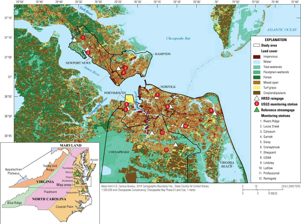
Map showing Hampton Roads monitoring stations and watersheds in which data were collected for this study. Station names are defined in table 1. Land cover categories from the Chesapeake Bay Program Office (2018). Some land-cover categories presented in figure 2 have been aggregated into coarser categories to improve visual presentation on this map. Coastal Plain Physiographic Province reference streamgages are shown in inset map and are described in appendix 1, table 1.1.
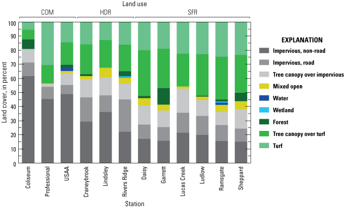
Percent of 9 land-cover classifications in the 12 monitored watersheds, ordered by land use and alphabetical order. Station names are defined in table 1. Land cover is based on the Chesapeake Conservancy, Chesapeake Bay Phase 6 High-Resolution 1-meter Land Cover Dataset (Chesapeake Bay Program Office, 2018).
The study was designed to establish background loading rates for TSS, total phosphorus (TP), and total nitrogen (TN); therefore, only watersheds with minimal stormwater best management practice (BMP) implementation were considered; the efficacy of BMPs was not evaluated. Watershed boundaries were delineated primarily on the basis of infrastructure maps provided by each jurisdiction. These maps included alignments of buried stormwater pipes and open conveyance channels, which did not always follow topographic features. Each stormwater network was physically walked to ensure the pipe network matched as-built diagrams. Data collection began at 10 monitoring stations on various dates throughout WY 2015 and at the other 2 stations in WY 2016. Real-time water-quality and streamflow data were recorded continuously at 5-minute increments throughout the study. Approximately 40 discrete water samples were collected at each station annually; these included a mix of event-targeted, high-flow “storm” samples and routinely scheduled “monthly” (typically low flow) samples. A complete annual (WY) timeseries was required for many of the analyses presented herein; therefore, data collected in WY 2015 are not included in this report.
Data Collection, Sampling, and Laboratory Analyses
The 12 monitoring stations were instrumented (fig. 3) to collect and record 5-minute measurements of water stage, WT, SC, and TB, collectively referred to as continuous data, which were transmitted to the USGS National Water Information System website (NWIS; U.S. Geological Survey, 2022) in near real time. Continuously collected 15-minute precipitation data were obtained from HRSD rain-gaging stations located near each of the monitoring stations. In both Hampton and Portsmouth, the two monitoring stations were associated with a single rain gage because of its proximity.
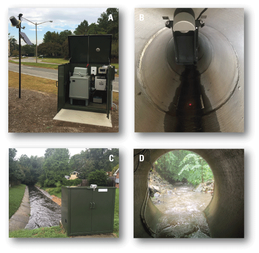
A, Monitoring station with equipment enclosure housing data loggers, automated sampler, and telemetry equipment at Storm Drain at USAA Drive at Norfolk, Virginia (Va.); B, in situ area-velocity meter mounted to the top of the stormwater pipe with laser beam visible on the water surface; C, equipment enclosure and trapezoidal concrete channel at Conveyance Channel at Ramsgate Lane near Great Bridge, Va.; and D, water flowing over equipment inside the stormwater pipe at Storm Drain at Rivers Ridge Circle, near Newport News, Va. Photographs by Aaron Porter, U.S. Geological Survey.
Standard USGS methods for continuously measuring and verifying water stage, measuring streamflow, and computing continuous timeseries of streamflow using either stage-discharge ratings or index-velocity ratings were followed (Rantz, 1982; Sauer and Turnipseed, 2010; U.S. Geological Survey, 2014a). A stage-discharge rating assumes free flow; however, this assumption was violated at many stations owing to backwater conditions. Although streamflow was computed on the basis of stage-discharge ratings at some stations, all stations were equipped with an in situ velocity meter, which was used to develop an index-velocity rating (Levesque and Oberg, 2012). Streamflow was calculated from the stage-discharge ratings at the Craneybrook, Daisy, Lucas Creek, Ramsgate, and Rivers Ridge stations, whereas index-velocity ratings were used at the Lindsley, Ludlow, Professional, and USAA stations. A combination of these methods to compute streamflow was used at the Coliseum, Garrett, and Sheppard stations, where backwater conditions occurred only during high flows, and in situ velocity meters performed poorly during periods of low streamflow. Despite attempts to avoid siting monitoring stations in tidally influenced locations, the effects of tide were observed occasionally at Coliseum and often at USAA. Reverse flow was not observed at either station, but during high tide a rise in water level downstream of the monitoring location created a backwater effect within the stormwater conveyance system, creating a tidal pattern in the stage data. This effect typically was not evident in the computed record of streamflow.
The operation and maintenance of continuous water-quality monitors was conducted by HRSD and USGS staff in accordance with published procedures (Wagner and others, 2006). During routine servicing visits to the stations, the instruments were cleaned and recalibrated when required on the basis of published thresholds. Data collected during these visits were used to apply corrections to WT, SC, and TB timeseries records for periods of suspected sensor fouling or calibration drift.
Base flow was sustained year-round at all stations by groundwater interchange through the concrete stormwater pipes. The chemistry of the water was characterized on the basis of analyses of monthly samples collected at each station in accordance with USGS methods (U.S. Geological Survey, 2006). All samples were analyzed for TSS and a suite of nutrient constituents (table 2). Monthly samples were collected by HRSD staff using a grab (dip) approach at the centroid of streamflow. All monitoring stations were sampled on the same day so as to limit variability in conditions across the stations; additionally, the order in which stations were visited was rotated each month. During each monthly sampling trip, three stations were randomly selected for the collection of an additional quality-assurance sample (two replicates, one blank). Additionally, from 28 to 40 event-targeted stormflow samples were collected at each monitoring station annually using an automated refrigerated sampler; these samples are referred to as storm samples throughout the report. The automated sampler was triggered to begin collection when a specified set of criteria were met. Criteria included a station-specific stage (water level) or streamflow threshold and a minimum time elapsed since the previous sample. Samples represented discrete points in time and were not composited to calculate an event mean concentration. For each storm event, a subset of the collected samples was manually selected by USGS personnel and retrieved by HRSD staff for delivery to the laboratory for analyses. Samples representing a range of conditions, including the rising, peak, and falling limbs of the storm hydrograph typically were collected for each event. All water-chemistry analyses were conducted by the HRSD Laboratory, as approved through the USGS Branch of Quality Systems Laboratory Evaluation Project (U.S. Geological Survey, 2014b). Samples were analyzed for concentrations of TSS, TP, orthophosphate (PO43-), total Kjeldahl nitrogen (TKN), nitrate plus nitrite (NO3-), and ammonia plus ammonium (NH3); concentrations of TN and total organic N (TON) were determined by calculation (TN is the sum of TKN and NO3-, TON is the difference between TKN and NH3).
Table 2.
Analytical methods used by Hampton Roads Sanitation District Laboratory for analyses of nutrients and suspended solids in water samples.Standard methods for the examinations of water and wastewater (Baird and others, 2017).
Statistical Analysis of Streamflow and Water Chemistry
Nonparametric analyses were used to describe statistical relations in water chemistry and streamflow data following methods published by Helsel and others (2020). Annual streamflow yield—the volume of streamflow generated per unit of drainage area—was calculated for each of the 12 monitoring stations as well as for 6 non-urban reference streamgages to inform hydrologic comparisons of watersheds of varying size and to investigate differences between land-use types. Non-urban reference streamgages in the Maryland, North Carolina, and Virginia Coastal Plain PP (see inset map on fig. 1) were selected to represent watersheds with low urban development (app. 1, table 1.1). Reference watersheds are orders of magnitude larger than those within the network because no comparable gaged watersheds were available at a sub-square mile scale.
Base-flow separation models and stream-flashiness metrics were used to investigate variability in streamflow characteristics across stations, land-use types, and seasons. Event-based analyses included those for stormflow duration, lag to peak, time to peak, stormflow volume, peak flow, runoff ratio, and rise rate, which were computed for extracted storm hydrographs. Spatial and seasonal patterns in water-chemistry data were evaluated using a nonparametric Kruskal-Wallace (Kruskal and Wallace, 1952) test and subsequent Steel-Dwass (Morley, 1982) post-hoc test for multiple comparisons (Critchlow and Flinger, 1991). The Steel-Dwass test is preferable to the more commonly used Wilcoxon method because Steel-Dwass controls for the overall experiment-wide error rate, thus reducing the probability of Type-1 errors (rejection of a true null hypothesis; Critchlow and Flinger, 1991). Monthly samples were collected on a pre-determined date and, by random chance, were occasionally storm-influenced. Summary statistics computed on monthly samples are intended to characterize base-flow conditions; therefore, these samples were instead included in the storm sample subset. The strength and statistical significance of correlation between metrics and response variables was evaluated using the nonparametric Spearman Rank correlation coefficient as defined by Spearman (1904). Where applicable, seasonal variability was tested by splitting the data by warm (April–September) and cool (October–March) seasons; in other instances, data were subset into four seasons based on solstice and equinox dates. Unless otherwise specified, the term “significant” is used throughout the text to denote a statistically significant difference based on a p-value less than or equal to (≤) 0.05.
Base-flow Separation Models and Storm-Hydrograph Separations
Base flow is the portion of streamflow derived from discharging groundwater. Stormflow is the portion of total streamflow contributed by direct surface, or overland, runoff to the stream channel, and to interflow, the water that initially infiltrates the soil surface and then travels through the unsaturated zone by means of gravity toward a stream channel. Separation of the base-flow and stormflow portions of total streamflow is useful for assessing the source of contaminants, the effects of urbanization on streamflow and water quality, and the characterization of TSS and nutrient loads by hydrologic condition (base flow versus stormflow).
Base-flow separations and storm-hydrograph extractions were conducted using modifications of the methods described by Hopkins and others (2020). Separation procedures were conducted on the 5-minute interval continuous streamflow timeseries at each station by applying the EcoHydRology R package (Fuka and others, 2018) using a 1-parameter digital filter with a filter parameter of 0.99 and 3 passes. The package provides output of total streamflow and a continuous timeseries of the proportion of base-flow and stormflow components. This output was used to calculate a base-flow index (BFI), which is the percentage of total streamflow contributed by base flow. Categorical separation of base-flow and stormflow periods was necessary for storm extractions, therefore further refinements were required. A storm period was first defined as a period when stormflow exceeded 0.25 cubic feet per second (ft3/s), total flow exceeded 0.50 ft3/s, and the slope of the hydrograph was greater than 0.10 ft3/s. To remove data for very small storms or slight fluctuations in streamflow erroneously included as storm events in the previous step, events lasting less than one hour were excluded from the analyses. Event selections were further refined by removing from the analyses the data for events with a rate of change (peak streamflow minus lowest streamflow value in the event) less than 0.1 ft3/s. Finally, because some storm events contained multiple peaks or occurred in quick succession because of intermittent precipitation, data for storms that occurred within a four-hour window were combined into a single event. A precipitation event typically precedes a streamflow response; therefore, each event was extended backwards one hour to identify the timing of peak rainfall and to quantify total event precipitation more appropriately.
Runoff Ratios
A ratio of stormflow to precipitation, hereafter termed “runoff ratio,” was calculated to evaluate the percentage of precipitation that flows directly to the storm conveyance. A runoff ratio provides a holistic examination of watershed processes, as it is a function of the interactions of precipitation, evapotranspiration, and infiltration (Ratzlaff, 1994). The runoff ratio can be influenced by impervious land cover, stormwater infrastructure, geology, watershed slope, and soil properties, such as depth, permeability and holding capacity. For example, impervious surface was found to increase runoff by 29 percent in areas with 50 percent impervious land cover (Lull and Sopper, 1969; Sanford and others, 2012).
Although runoff ratios are a commonly reported statistic, the use of this terminology and the methods used to derive it are inconsistent throughout hydrologic literature. A runoff ratio may be calculated by including either total streamflow or separated stormflow (Bell and others, 2016; Ratzlaff, 1994), and either total precipitation or throughfall, precipitation that penetrates through tree canopy and reaches the soil surface (Blume and others, 2007; Brown and others, 1999). Runoff ratios computed based on stormflow only are highly affected by the hydrograph separation method used (Blume and others, 2007); thus, care must be taken before comparing the results of different studies. In this study, the runoff ratio was computed on total streamflow during periods defined as storms, which were identified according to the base-flow separation and stormflow hydrograph methods described above, in the following equation:
whereCr is the runoff ratio,
SFy is the area-normalized event-based stormflow volume, and
Py is the area-normalized event-based precipitation volume.
The factors SFy and Py were calculated as the sum of streamflow and precipitation during each identified storm event, respectively. Watershed-specific 15-minute precipitation data were obtained from the nearest HRSD rain gage. Event-specific runoff ratios were calculated at the 12 monitoring stations for WY 2016 through 2020.
Flashiness Index
Flashiness, or the rate of change in streamflow, is a metric used to quantify a watershed’s response to precipitation (Baker and others, 2004). Urban development and associated impervious surfaces and engineered stormwater conveyances typically increase the flashiness of a watershed. The Richards-Baker flashiness index (RBI) was applied to mean hourly streamflow data collected in this study following the methods published by Baker and others (2004). Baker and others (2004) used mean daily streamflow when developing this method; therefore, care should be taken when comparing results across studies. The RBI measures oscillations in streamflow relative to total streamflow. This index is dimensionless and is positively correlated with the flashiness of streams in a basin. The index is calculated as
whereEvent-Based Streamflow Metrics
Six event-based streamflow metrics that characterize the duration, magnitude, volume, timing, and rate of change of storm hydrographs were calculated to investigate spatial and seasonal patterns in watershed hydrology during periods of runoff. Two metrics that describe stormflow durations were (1) total-event duration, herein referred to as “duration,” calculated as the total time in hours from the beginning to the end of the storm event; and (2) the length of time from the beginning of the event to peak streamflow, herein referred to as “time to peak.” The magnitude of each event was described by quantifying peak streamflow volume and then normalizing by watershed area to allow inter-station comparisons, herein referred to as “peak flow” and expressed in units of cubic feet per acre (ft3/acre). Likewise, the volume of stormflow was computed for each event as the total streamflow volume per unit area over the duration of the event, herein referred to as “event yield.” The timing of each runoff event was calculated as the time in hours between peak precipitation and peak streamflow and is herein referred to as the “lag to peak.” Lag to peak can be conceptualized as the fingerprint of the watershed, as it reflects the storage and speed at which water moves from land to stream. Lag to peak is a function of natural factors such as soil characteristics and basin slope and disturbance factors like impervious surfaces and channelization that reduce surface storage and increase in-stream velocity (Leopold, 1991). The rate of change during the rising limb of each stormflow hydrograph was calculated as the “rise rate,” or peak streamflow yield divided by the time to peak, expressed in units of ft3/acre per hour (ft3/acre/hour). Under similar meteorological conditions, a storm event in an undeveloped watershed would have a longer time to peak, total duration, and lag to peak, and lower RBI, rise rate, peak flow, and event yield than a stream in a highly urbanized landscape because of greater infiltration, retention, and longer and less direct flow paths from uplands to the stream channel (Leopold and Dunne, 1978).
National Stormwater Quality Database Comparisons
Median concentrations of sediment and nutrients in samples collected in this study were compared to their concentration in the National Stormwater Quality Database (NSQD) version 4.02 as well as to a subset of those data collected in the Hampton Roads region to provide additional context to the interpretation of these results (Pitt and others, 2018). The NSQD is an EPA compilation of stormwater-quality data of the United States and contains data collected from more than 600 outfall monitoring locations. The NSQD contains data from Phase 1 National Pollution Discharge Elimination System municipal monitoring programs, USGS studies, BMP database outfall data, state and academic research, the Nationwide Urban Runoff Program, and other sources. Version 4.02 of the NSQD contains data collected from 1977 through 2015. A subset of those data collected in Hampton Roads from 1990 through 2001 was also used for comparison. Although these data were collected outside of the current study period, they provide additional context to measured concentrations, highlight potential spatial variability in water quality, and may allude to changes over time; differences in concentrations across these datasets, however, should not be interpreted as indicative of a trend. The NSQD stations were subset to include only those data representing residential or commercial watersheds to provide consistency with data from land-use types assessed in the current study.
Handling of Censored Data
Concentrations of TSS, PO43-, and NH3 were below laboratory instrumentation detection limits in some samples. Concentrations less than the method detection limit (MDL), known as left-censored data, indicate that a concentration is somewhere between zero and the MDL, but the actual concentration is unknown. Censored values that are deleted or substituted with a constant value, such as one-half of the reporting limit, may produce biased results and introduce patterns not present in the original dataset. To properly handle censored data, nonparametric methods were used, such as the Spearman rank-order correlation (Spearman, 1904), Kruskal-Wallace and Steel-Dwass tests, and robust regression on order statistics, which do not rely on calculating a mean or standard deviation from an assumed distribution, but instead perform statistical analyses on the ranks of data.
Concentrations less than the MDL are stored in the USGS NWIS at a reporting limit that is higher than the MDL. This handling of censored results can produce an upward bias in the data (Helsel, 2005) and was resolved by recoding censored results to the MDL. Monthly and storm-sample data were analyzed by using the Nondetects and Data Analysis for Environmental Data (NADA) version 1.1 package for R v. 3.6.3 (R Core Team, 2017). Load computations were performed on the censored data as originally reported in NWIS, because the rloadest software—an R implementation of LOAD ESTimator (LOADEST) FORTRAN program (Runkel and others, 2004)—contains an algorithm to properly fit these data and eliminate bias in the estimation of model coefficients.
Cross-Correlation Analysis
The relation of peak concentration of a constituent (or a constituent surrogate such as TB) and peak streamflow can help inform the source of that constituent. These relations typically are evaluated by examining the graphical pattern of the constituent, the streamflow hysteresis loop. These relations typically form a loop of varying shape and direction. The wider the loop, the more concentration varies across the storm event at any given value of streamflow. When concentration is greater on the rising limb of the storm hydrograph at a given unit of streamflow, the pattern is referred to as a clockwise loop (Landers and Sturm, 2013; Bussi and others, 2017). A clockwise loop suggests the first-flush phenomenon, which has been well documented in studies of highly urban watersheds (Bertrand-Krajewski and others, 1998; Deletic, 1998; Geiger, 1987; Gupta and Saul, 1996; Lee and others, 2002), and suggests the primary source is at or nearby the measurement point, such that the constituent is primarily input to the stream on the rising limb of the hydrograph. Conversely, a counterclockwise loop indicates greater concentration on the falling limb of the hydrograph and suggests a source that is farther upland of the measurement point and requires a longer time of travel (Williams, 1989).
Although hysteresis loops can be informative, they are event-specific, can be difficult to interpret in flashy streams where few data points are collected during the rising limb of the hydrograph, and are not well suited to evaluation of hundreds of events simultaneously. Cross-correlation analyses were used to quantify the TB-streamflow, TP-streamflow, and TN-streamflow relations for all extracted storms and were interpreted in the context of hysteresis loops. Total suspended solids concentrations could be used for this analysis, but TB was preferred because it (1) is a strong surrogate for TSS (Gippel, 1995; Jastram and others, 2009; Jones and others; 2010), and (2) can be continuously measured. These analyses provided a simultaneous evaluation of hysteresis patterns in hundreds of station-event specific storms to investigate patterns in concentration-streamflow relations and the timing and source of inputs. The cross-correlation function calculates multiple correlations between timeseries of streamflow and constituent concentration data, where one variable is adjusted forward and backward by sub-hourly increments while the other is held constant. The maximum correlation coefficient of these iterations is identified and represents the time offset at which streamflow and constituent concentration (or water-quality parameter) peaks are aligned. The function was calculated using the R stats package (v. 3.5.1) in R v. 3.6.3 (R Core Team, 2017).
Mass-Volume Curves
The first-flush phenomenon was first coined by Metcalf and Eddy (1916) and has since been used to indicate a disproportionately high concentration or mass transport of a constituent in the initial phase (rising limb) of a storm event. Mass-volume (M[V]) curves are used to investigate patterns in constituent transport across the storm hydrograph and to objectively identify a first flush. Mass-volume curves were computed for each extracted storm event using continuous measurements of streamflow and unit value (5-minute interval) predictions of constituent load derived from surrogate regression models. For each storm event, the cumulative, total mass, cumulative, and total stormflow volume was computed. A dimensionless cumulative mass (L) and stormflow volume (F) was then calculated using the following equations described by Lee and others (2002):
whereL is the dimensionless cumulative constituent mass,
m is the mass of constituent transported up to time t in the storm event,
t is time, and
M is the total mass transported during the event,
F is the dimensionless cumulative stormflow volume,
v is the volume of stormflow transported up to time t in the storm event,
t is time, and
V is the total volume of stormflow transported during the storm event.
Geiger (1987) proposed a criterion to define the strength of a first flush by calculating the difference (Δ) between L and F at each observation (t) during the storm event. The difference is computed for each observation as
For each storm, the maximum Δ (ΔMax) is used to quantify the relation between the curve and the bisector (45-degree, 1:1 line). A linear 45-degree line indicates that mass transport remains constant throughout the storm event. Helsel and others (1979) defined the first flush as occurring when the M(V) curve is above this bisector; however, Geiger (1987) recommended a more quantifiable definition by identifying a first flush when ΔMax is greater than or equal to 0.2. Alone, this definition is limited because it does not indicate where on the M(V) curve ΔMax occurred. Gupta and Saul (1996) improved Geiger’s definition by including an additional coefficient, cumulative percentage of time (T = cumulative time / total time). This method allows for a more objective and repeatable interpretation of the M(V) curve by defining the first-flush phase as the period up to ΔMax, quantifying the percentage of mass (Y) transported in a given percentage of volume (X), and providing the time (T) that it took for that to occur. For each storm event, ΔMax was regressed against X, Y, and T, and for each station the mean value of X, Y, and T was computed. Criteria for the percent mass transport over a given percent of stormflow volume (for example, 80 percent of the mass in the first 30 percent of volume) used to define a first-flush event vary substantially throughout the literature and are selected arbitrarily; however, selection of any a priori criteria allows for repeatable evaluation of the first flush.
Total Suspended Solids and Nutrient Estimation Models
Total suspended solids and nutrient concentration and load timeseries were computed for the 12 monitoring stations with regression models that include continuous water-chemistry and streamflow data as explanatory variables. Annual loads were converted to yields, or the load per unit drainage area, to remove the effect of watershed size and allow for comparisons between stations. Methods and rationale for estimating TSS and nutrient concentrations and loads using this “surrogate” regression approach have been well documented (Jastram and others, 2009; Jastram, 2014; Nash and Sutcliffe, 1970; Porter and others, 2020; Rasmussen and others, 2009a; Robertson and others, 2018; Schilling and others, 2017), so only a summary of pertinent details is presented here.
Continuous records of streamflow data were available at 5-minute intervals; however, concentration data were available only from discretely collected samples that provide a “snapshot in time” of constituent concentration. To compute a load at each instantaneous timestep (5-minute interval), the constituent concentration must be estimated for all timesteps when samples are unavailable. To this aim, water-chemistry parameters that can be continuously measured were used as surrogates for the estimation of concentration.
Station-specific regression models were developed for TSS, TP, PO43-, TN, TON, TKN, and NO3- concentrations using JMP 14 software (SAS Institute, Cary, N.C.). Models were calibrated using discrete concentration data available from analyses of both monthly and storm samples as the response variable. For each model, the following explanatory variables were considered: streamflow and the water-quality variables SC, WT, TB; temporal variables trend and season; and a binary indicator variable for hydrologic condition (base flow or stormflow). The binary variable was included when the slope of the surrogate—concentration relation was consistent across hydrologic condition, but the y-intercept differed. In select cases, the slope of this relation also differed across hydrologic condition; therefore, an interaction term—natural logarithm TB times hydrologic condition—was included.
Models were selected to maximize explanatory power, while minimizing systemic errors (bias) and random errors (variance) using a suite of criteria described by Helsel and others (2020), including (1) prediction error sum of squares (Allen, 1974); (2) Nash-Sutcliffe efficiency index (Nash and Sutcliffe, 1970); (3) model bias percentage (Bp) that indicates over- or underestimation; (4) partial load ratio, a ratio of the sum of the estimated loads to the sum of the observed loads (Stenback and others, 2011); (5) Mallow’s Cp (Mallows, 1973); (6) variance inflation factor; (7) autocorrelation; and (8) analyses of model residuals. Some diagnostics for load models are inflated because most of the variability in loads is driven by variability in streamflow, which is included as part of the dependent variable in all models. Therefore, diagnostics of both the load and concentration models were evaluated. Concentration and load models are identical except for the intercept and the coefficient for the streamflow term. Although the coefficient of determination (R2) values of load models are deceptively high, other load model diagnostics such as the Nash-Sutcliffe efficiency index and model Bp are important, given that loads, rather than concentrations, are the primary focus of this study. Instantaneous constituent loads were computed from the selected models using rloadest in version 0.4.5 of R Studio (R Core Team, 2017; Lorenz and others, 2015). Instantaneous load timeseries were then aggregated to an annual (WY) timestep.
The adjusted maximum likelihood estimator (AMLE) algorithm was used to properly fit models for constituents with censored observations. The AMLE method also corrects for retransformation bias introduced because of the nonlinear relation of predicted concentrations in natural logarithm transformed and original units (Cohn and others, 1992). The standard error of prediction also was calculated for each load and used to compute 95-percent confidence intervals around each load estimate.
Data Storage
All continuous stage and streamflow data (5-minute interval) and basic water-quality parameters (5-minute interval), and discrete laboratory-analyzed water samples collected at the 12 monitoring stations are available in NWIS (U.S. Geological Survey, 2022). Those data, or results of subsequent analyses, that could not be stored in NWIS are available as a data release (Porter, 2022). The data release includes computed unit values for RBI flashiness indices, annual streamflow metrics—streamflow volume, base-flow separations, runoff ratios, peak streamflow, annual nutrient and suspended-sediment loads, load model calibration and estimation files, and HRSD precipitation data.
Watershed Hydrology
Streamflow is perhaps the most fundamental factor affecting water quality in the stream; therefore, it is critical to properly characterize and understand the hydrologic regime of a stream when synthesizing water-quality data. Patterns in streamflow variability over time—from minutes to years—are collectively referred to as the hydrologic regime of a stream. The hydrologic regime can be characterized by such factors as the volume of base flows, magnitude and duration of stormflows, and degree of flashiness, among others. The hydrologic regime is affected by climate, land use, land cover, geology, soils, and watershed size. In particular, changes in the extent of impervious land cover have been linked to changes in watershed hydrology (Jayakaran and others, 2014; O’Driscoll and others, 2010; Paul and Meyer, 2001; Rose and Peters, 2001; Walsh and others, 2005b), and the effect of urbanization on peak flows and storm recurrence frequencies may be more pronounced in Coastal Plain PP watersheds than in the adjacent Piedmont PP (Utz and others, 2011). These authors also hypothesized that the geology, topography, and soils of the Piedmont PP facilitate rapid runoff even in undeveloped watersheds, but because the low relief, deep unconsolidated sediments, and permeable sandy soils of the Coastal Plain PP can better attenuate this runoff, disturbance of natural runoff patterns and processes by impervious cover may have a greater impact in the Coastal Plain. Precipitation conditions and streamflow metrics highlighting spatial and temporal runoff patterns were analyzed to better understand the factors affecting watershed hydrology and water quality in Hampton Roads.
Precipitation
Mean annual rainfall totals from the 10 precipitation stations were at or below the 5-year mean in 4 out of 5 years, with the lowest mean annual rainfall occurring in WY 2018 and the highest in WY 2016 (fig. 4; Porter, 2022). Total annual rainfall varied spatially across the 10-station precipitation network (mean range is 16.4 inches [in.]); the greatest variance occurred in the wettest year (WY 2016; minimum is 52.6 in.; maximum is 72.7 in.; fig. 5). Variance between stations reflects the large geographical extent of the study region and highlights the importance of utilizing local rainfall data when interpreting patterns in streamflow and water quality. In all years, approximately half of the total annual precipitation fell on days with high-intensity or high-volume (greater than [>]1.0 in.) events. In WY 2016, Tropical Storm Julia produced an average of 9.3 in. precipitation across the network over a 4-day period, and Hurricane Joaquin delivered 4.5 in. over a 3-day period. In WY 2017, an average of 7.7 in. of rain fell during Hurricane Michael, ranging from 6.8 in. to 9.4 in. across the network and exceeding the 100-year, 6- and 12-hour peak rainfall recurrence interval at most stations (Hampton Road Sanitation District, 2016; National Oceanic and Atmospheric Administration, 2022a). In the fall of WY 2019, Hurricane Sally produced an average of 4.7 in. of rainfall over 2 days across the network. An additional 69 unnamed storm events produced daily rainfall totals greater than 1.0 in., two-thirds of which occurred in the warm season (April–September). High-precipitation periods can have pronounced effects on hydrologic and water-quality conditions with the potential for conveying substantial loads of sediment and nutrients.
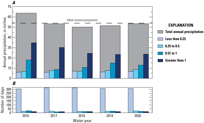
A, Annual precipitation data from 10 Hampton Roads Sanitation District precipitation stations for water year 2016 through 2020 and inset with annual totals generated by daily precipitation events. B, the number of days annually that each type of daily rainfall event occurred. A water year begins October 1 and ends September 30 of the following year.
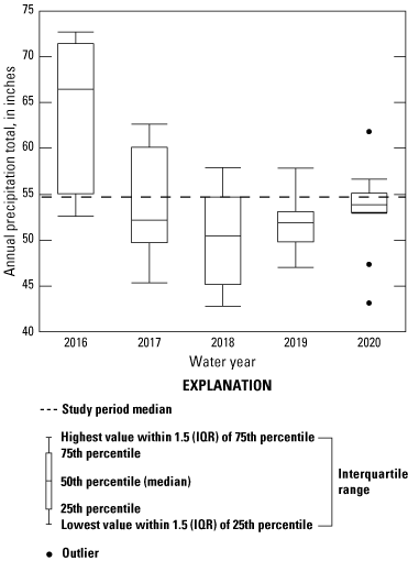
Boxplots showing the variation in total annual precipitation at the 10 Hampton Roads Sanitation District precipitation stations. A water year begins October 1 and ends September 30 of the following year.
Streamflow
Median annual streamflow yields were highest at the 3 COM watersheds—Professional, USAA, and Coliseum: 242,000, 237,000, and 140,000 ft3/acre, respectively (fig. 6). High-density residential watersheds yielded more streamflow than SFR, a difference that was driven by the yields at Craneybrook and Rivers Ridge. Single family residential watersheds were the lowest flow-yielding land use, and exhibited only a weak statistical difference (p = 0.059) from the reference watersheds, despite substantially higher levels of development and impervious cover in the SFR watersheds. Seasonal variability in streamflow yields reflect meteorological patterns. Yields were greatest in the summer, a consequence of high-intensity storms that generated high volumes of runoff. Yields were lower in winter and spring, when low-pressure systems produced longer duration but lower intensity storms that resulted in moderate volumes of runoff, greater infiltration, and higher base flows. Streamflow yields were lowest in the fall, the season when rainfall typically is low.
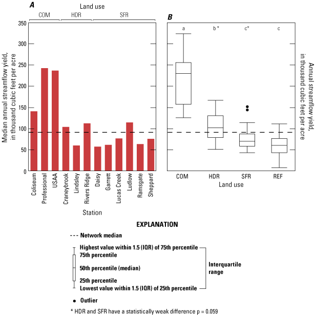
A, Bar plot of median annual streamflow yield at the 12 monitoring stations. B, boxplots showing variation in annual streamflow yields grouped by land-use type for water year 2016 through 2020. Non-matching letters denote statistical significance based on p less than or equal to 0.05. A water year begins October 1 and ends September 30 of the following year. Station names defined in table 1. REF represents six reference Coastal Plain Physiographic Province streamgages described in appendix 1, table 1.1.
A reduction in base flow and an increase in flashiness are the most common effects of land development on streamflow (Hirsch and others, 2010; Poff and others, 1997). Base flows are sustained in concrete stormwater conveyance systems as a result of hydraulic interchange with the surrounding saturated-unsaturated zone through the cracks, joints, and pore space in the concrete. When the water table is above (at higher elevation than) a portion of the pipe, groundwater inflow occurs because the pressure outside of the pipe exceeds that within it; alternatively, when the water table drops below the elevation of the pipe, outflow from the pipe can occur (Peche and others, 2019). Inflow of groundwater into the stormwater conveyance system can reduce recharge and result in lowering of the groundwater table by several inches (Thorndahl and others, 2016). Base flows may also contain leakage from potable-water pipes, which typically have leakage rates of 20 to 30 percent, and from sanitary sewer lines, which are commonly constructed in close proximity to stormwater conveyances (Kaushal and Belt, 2012; Garcia-Fresca, 2007). Monitored stormwater conveyances in the Hampton Roads study area had significantly lower annual BFIs than non-urban reference streams (fig. 7A). Single-family residential watersheds had significantly higher annual BFI than the COM and HDR stations, but only two of the SFR stations (Sheppard and Ramsgate) were baseflow dominant (> 0.5) in most years. Streams in the Coastal Plain PP naturally have high base flows (greater than or equal to [≥] 75 percent of total flow) because of low surface runoff, the result of high infiltration rates in sandy soils and low topographic slope (Sanford and others, 2012). In urbanized areas, disturbance factors such as soil compaction, loss of vegetation, construction of impervious surfaces, and the direct channelization of runoff to stormwater conveyance systems reduce groundwater recharge, decrease infiltration, and reduce storage and release of base-flow sustaining groundwater to streams (Rose and Peters, 2001).
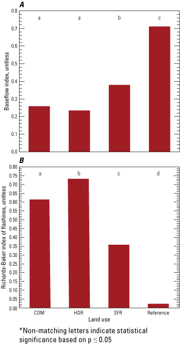
A, Median base-flow indices and B, Richards-Baker flashiness indices by land-use type. Land use categories defined in table 1. “Reference” represents 6 Coastal Plain Physiographic Province reference streamgages described in appendix 1, table 1.1.
Annual RBI scores were computed for each of the 12 monitoring stations and the 6 reference streamgages. Flashiness scores ranged widely across the 12-network stations from 0.83 at Lindsley to 0.25 at Ludlow. Flows at stations in HDR and COM watersheds were flashiest, with median RBI scores of 0.73 and 0.62, respectively, followed by flows at stations in SFR watersheds (0.36), and in the reference watersheds (0.02; fig. 7B). Streams in natural Coastal Plain PP watersheds are typically more stable (less flashy) than streams in other PPs because of high soil permeability, low topographic gradient, wide stream channels, and broad alluvial floodplains. High flashiness scores computed across the monitoring network are likely related to the engineered stormwater systems that serve these watersheds, which disconnect surface water hydrological processes from the natural land attributes that typically shape the hydrologic regime in the Coastal Plain PP. Flashiness is also likely related to specific design characteristics of the constructed stormwater system, watershed size, and the degree of impervious cover. These systems are engineered to export water quickly and efficiently; however, to achieve this aim channels are built on a higher gradient and with a more direct flow path than natural Coastal Plain PP streams. Differences in degree of impervious cover and in watershed size may explain much of the spatial variability observed across different land-use types. Single family residential watersheds were larger, had less impervious cover, and greater composition of land cover attributes (such as turf grass and tree canopy) that promote uptake, retention, and interception of runoff than did HDR or COM watersheds. A significant seasonal effect was present at all stations, with greater flashiness observed in warm months than in cool months, reflecting meteorological patterns—higher intensity convective systems such as thunderstorms in warmer months and lower intensity low-pressure systems in cool months.
An evaluation of flashiness across 41 USGS streamgaging stations, which included the 12 network stations in this study, CB-NTN, Coastal Plain PP reference stations, and multiple other urban monitoring stations in Fairfax County, Virginia and the City of Roanoke, Virginia, was conducted to better understand factors affecting stream flashiness across a wide range of watershed types (small versus large, urban versus non-urban). This analysis revealed strong correlations between RBI scores and both watershed size and impervious cover (fig. 8A, B; Porter, 2022). Watershed area and impervious cover are themselves highly correlated, so a stepwise linear regression analysis was used to identify the primary driver. Although watershed area likely influences flashiness, impervious cover was the strongest driver across these 41 monitored watersheds, explaining 84 percent of spatial variability. Flashiness increased by approximately 10 percent for every 10 percent increase in impervious cover, a relation that was consistent across different drainage network types (for example, earthen streams versus engineered conveyances).
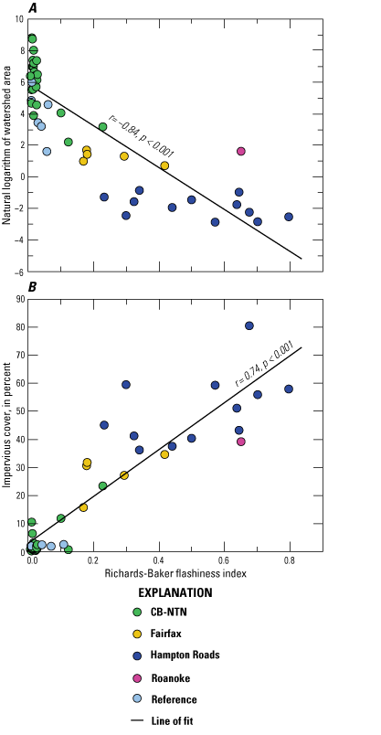
The relation of Richards-Baker flashiness index (RBI) to A, watershed area and B, impervious land cover. CB-NTN is the Chesapeake Bay non-tidal network. Reference represents the non-urban Coastal Plain reference stations.
Streamflows in most of the study watersheds were stormflow dominated. To gain greater insight into this component of the hydrologic regime, storm hydrographs were extracted from continuous records of streamflow and used to characterize spatial and temporal variability in runoff response. In total, 4,720 individual storm hydrographs were extracted from the data for the 12 monitoring stations (200 to 535 storms per station). For each storm, the total streamflow yield, peak flow, runoff ratio, rise rate, lag to peak, time to peak, and event duration were computed (table 3). Higher values for metrics that describe volume, magnitude, and rate of change in flow, such as event yield, peak flow, RBI, runoff ratio, and rise rate typically are related to increasing urbanization (Paul and Meyer, 2001). Generally, as magnitudes of these metrics increase, so does the potential for constituent transport, depending on the pollutant and its source (O’Driscoll and others, 2010). Conversely, longer duration, lag to peak, and time to peak commonly result in greater constituent retention and are indicative of a more stable hydrologic system.
Table 3.
Median event-based streamflow metrics at the 12 monitoring stations and network summary.[Station names and land-use types are defined in table 1. All monitoring stations, unless otherwise stated, are at storm drains. ft3/acre, cubic foot per acre]
Event yield was positively related to precipitation volume at all stations, but the slopes of these relations varied by land use. Slope was steepest in COM watersheds followed by lesser slopes in HDR and SFR (fig. 9; app. 1, table 1.2). This demonstrates that differences in runoff, and consequently differences in streamflow, are generated by an equal volume of rain falling across these three land-use types, and likely reflect differences in impervious cover, and in SFR watersheds in particular, landscape features like lawns and trees that promote infiltration and increase retention. Median runoff ratios varied widely across stations; from 10 to 72 percent of precipitation ran directly to the conveyance system as direct runoff and was positively related to watershed imperviousness (fig. 10). On average, approximately 10 percent of precipitation becomes direct runoff in forested watersheds versus 55 percent in watersheds with 75–100 percent imperviousness (Arnold and Gibbons, 1996). Runoff ratio values less than 10 percent are common in the Coastal Plain PP (Sanford and others, 2012). These differences reflect lower infiltration and evapotranspiration with increasing imperviousness.
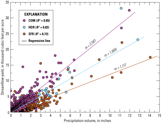
Event-based streamflow yield compared to event-based precipitation volume across the three land-use types from water year 2016 through 2020. A water year begins October 1 and ends September 30.
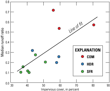
The relation between watershed impervious cover and median annual runoff ratio at each monitoring station for storm events occurring in water years 2016 through 2020. A water year begins October 1 and ends September 30 of the following year. Points are colored by land-use type and defined in table 1.
Principal component analysis was used to explore patterns in event-based hydrologic metrics across stations, land-use types, and seasons (fig. 11). Principal components (PC) 1 and 2 explained a combined 83.3 percent of the variability in the data. The strongest loadings to PC1 included metrics describing the magnitude (peak) and rate of change (rise rate and lag to peak) in streamflow (app. 1, table 1.3). The strongest loadings to PC2 included event yield, runoff ratio, and time-based metrics like duration and time to peak.
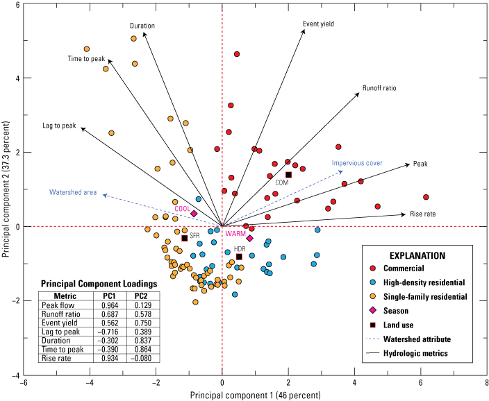
Principal component analysis (PCA) on correlations of seven event-based hydrologic metrics calculated on extracted periods of stormflow, with supplementary variables for season (warm season is April through September and cool season is October through March) and land-use type (commercial [COM], high density residential [HDR], and single-family residential [SFR]).
Commercial watersheds (Coliseum, USAA, and Professional) had the highest event yields, runoff ratios, and peak flows; rise rate was also highest at Coliseum and Professional. Variability between SFR and HDR watersheds was less pronounced, though storms at SFR stations typically were longer in duration and time to peak, and had a longer lag between peak precipitation and peak streamflow. Average storm duration, time to peak, and lag to peak were longest at the two largest watersheds, Ramsgate and Ludlow, which indicate slower export of runoff. This pattern was likely affected by two factors: (1) larger watershed area, which inherently results in a longer flow path, and (2) a high proportion of pervious land cover, such as lawn turf and tree canopy (table 4). These land-cover features can serve to disconnect non-road impervious surfaces like rooftops from stormwater inlets. Building on previous analyses, these results suggest a greater volume and rate of runoff in watersheds with high impervious cover that consequently lack areas for retention and infiltration. In particular, characteristically short lag to peak and high-rise rate at COM stations suggest a short and direct path of travel from the land surface to stormwater conveyances. It is important to note that the correlations do not imply causation, as additional factors may be driving differences in streamflow metrics.
Table 4.
Spearman rank-order correlation coefficients between selected land-cover attributes and event-based hydrologic metrics.[Significance is based on p less than or equal to 0.05). *, statistically significant positive correlation; †, statistically significant negative correlation; −, negative]
Seasonal variability was evident in the spread of warm and cool season variables on PC1, suggesting greater magnitude and rate of change in warm months, and longer duration, time to peak, and lag to peak in cool months. Similar to stream flashiness, temporal differences in event-based metrics likely are related to seasonal meteorological patterns, such as the duration, intensity, and recurrence of precipitation events. Unlike metrics describing event magnitude, timing, and rate of change, runoff ratios and event yields did not differ across seasons. This suggests that although the hydrograph was less flashy in the cool months, the percentage of precipitation that reaches the storm conveyance and consequently the volume of runoff transported out of the watershed during a storm event is consistent year-round. Consistency in yield can be explained by the seasonal nature of precipitation events in the Mid-Atlantic region of the United States—short duration-high intensity events in the warm season and long duration-low intensity events in the cool season. Both types of storms can deliver the same volume of rain across a watershed, and in doing so produce a similar volume of streamflow, but more critically, the rate at which runoff is produced differs, and may affect the magnitude of event-derived sediment and nutrient loading. These patterns highlight the importance of considering seasonal differences in storm-event hydrology as part of stormwater-management planning and evaluation.
Water-Quality Conditions
Spatial and temporal patterns in a suite of water-chemistry constituents were defined to characterize water-quality conditions in selected stormwater conveyances in Hampton Roads and to explore how variability in those conditions may be related to seasonal effects, land use, and other watershed properties. This report includes results of the analyses of all data collected in the Hampton Roads study area from October 2016 through September 2020. Continuous data collection began at eight of the monitoring stations by the start of WY 2016 and at the other 4 stations at various dates later during that year. Discrete water-quality samples—a total of 2,341—representative of the range of observed hydrologic and environmental conditions were collected from all 12 stations during the period of study. Loads were computed for seven constituents at each monitored watershed to provide a holistic evaluation of the complex, integrated watershed processes that affect both water quantity and quality (Barber and others, 2006). For the stations Craneybrook, Garrett, Lucas Creek, Professional, Ramsgate, Rivers Ridge, Sheppard, and USAA, loads and yields were computed for WYs 2016 through 2020; for stations Coliseum, Daisy, Lindsley, and Ludlow, loads and yields were computed for WYs 2017 through 2020 (Porter, 2022).
Quality-assurance samples were collected concurrent with environmental samples to ensure repeatable and unbiased results. Sixteen blanks and 40 sample replicates were collected during monthly sampling trips. Blank samples were consistently ‘clean’—their analyses did not indicate any contamination nor any systemic issues with sampling equipment or with either sampling or laboratory procedures. In general, variance between replicate samples was negligible; however, a few TSS replicates were substantially different, and these samples were excluded from subsequent analyses. Analytical results for replicate samples for TN, TP, and TSS were highly correlated (r = 0.96, r = 0.93, and r = 0.84, respectively), indicating measurements were accurate and repeatable.
Water Temperature
Water temperature (WT) is a fundamental property of water quality given its role in regulating chemical and biological reactions and governing the structure of aquatic communities (Demars and others, 2011; Hillebrand and others, 2010; Mulholland and others, 2001). Water temperatures in the stormflow and monthly samples ranged from 2.0 to 31.2 degrees Celsius (°C) and from -1.3 to 35.2 °C in the continuously collected data. Water temperatures were seasonally variable, with a median networkwide cool season (October–March) value of 13.9 °C and warm season value of 21.8 °C. A positive correlation (r = 0.59, p = 0.044) was observed between WT and degree of impervious land cover in a watershed. This relation has previously been linked to increased runoff, decreased base flows, and the low albedo, or reflectivity, of roads, sidewalks, and buildings that gain and hold more heat, and consequently increase the temperature of overland runoff (Galli, 1991; O’Driscoll and others, 2010). Unlike the findings in studies of earthen streams in the urban environment (Hyer and others, 2016; Jastram, 2014; LeBlanc and others, 1997; Porter and others, 2020), diel fluctuations in daily water temperature were minimal at most stations, and this pattern was consistent throughout the year (fig. 12). Diel Fluctuations were larger at the three stations most exposed to ambient air: Ramsgate (open channel), and Ludlow and Daisy (storm drains connected to road culverts). Daily fluctuations in WT at all stations were attributed to similar oscillations in air temperature and were greatest in late winter and early spring because of heating by solar radiation prior to leaf out of the tree canopy (Porter and others, 2020; Johnson, 2004). The other nine stations, which are located in buried concrete storm pipes, are more buffered against changes in ambient air temperatures. As a result, WT also was warmer at these stations during cool season months. This difference highlights an important physicochemical difference in water flowing through earthen streams versus engineered stormwater conveyances that may affect water quality. Warmer temperatures stimulate microbial respiration, which in turn promotes the uncoupling of nutrients from organic matter and can increase the export of bioavailable P and N (Demars and others, 2011). This effect may be most evident during periods of base flow when residence time is longer and therefore biogeochemical transformations of organic substrates can occur within the storm conveyance network (Kaushal and Belt, 2012).
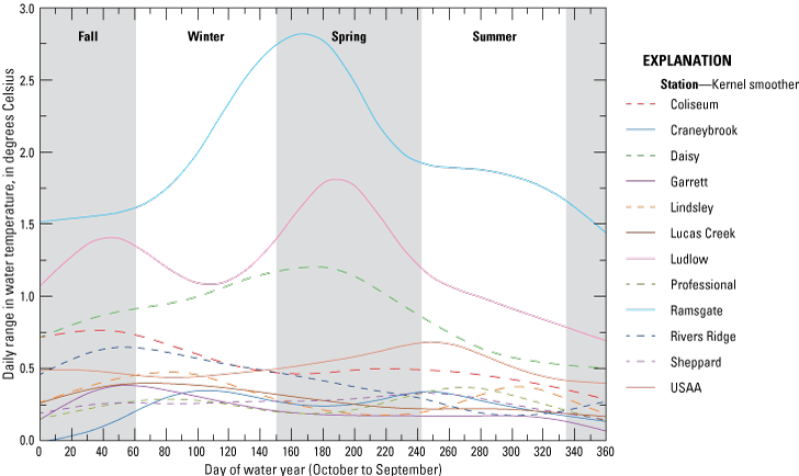
Daily ranges in water temperature, summarized from continuous (5-minute interval) measurements at the 12 monitoring stations and plotted against day of the water year, where 1 is October 1 and 365 is September 30 in a nonleap year.
Specific Conductance
Specific conductance (SC) is a measure of the ability of water to conduct electric current, corrected for temperature (typically 25 oC) and provides an indication of ion concentration in water (Hem, 1985). Streams in less developed areas of the Coastal Plain PP typically have mean SC values less than 100 microsiemens per centimeter (µS/cm) because of the relative abundance of quartz sand and lack of soluble minerals in the soils and underlying geologic formations (Sanford and others, 2012). In areas where temperature, geology, and precipitation are relatively constant, SC serves as an indicator of urban impacts on stream chemistry (Paul and Meyer, 2001).
The ionic strength of freshwater streams has increased across the United States because of anthropogenic influences in recent decades (Griffith, 2014). Freshwater salinization is a growing concern in urban watersheds, and it has been estimated that a significant change in the degree of salinization has occurred in 37 percent of streams in the contiguous United States (Kaushal and others, 2018). Salinization can degrade stream and drinking-water quality through the mobilization of N and P from soils (Haq and others, 2018; Steele and Aitkenhead-Peterson, 2013), the leaching of metals from water-conveying infrastructure (Kaushal, 2016; St. Clair and others, 2016), and numerous negative impacts on aquatic life (Corsi and others, 2010). Factors affecting ion concentrations, and thus SC, include temperature and geologic weathering (Hem, 1985), saltwater intrusion (Kaushal and others, 2021), and the discharge of wastewater to streams or groundwater (Paul and Meyer, 2001; Potter and others, 2014). Road anti-icer and de-icer applications, in particular, have been linked to elevated ion concentrations, such as sodium and chloride, in streams (Shanley, 1994). These applications are considered a major contributor to freshwater salinization in the urban environment and have been documented throughout the northeastern and southeastern United States (Kaushal and others, 2005; Moore and others, 2020).
Weathering of concrete building materials also has been linked to salinization and other changes in stream chemistry and is particularly evident in regions underlain by a dense network of concrete stormwater infrastructure (Kaushal and others, 2017). Weathering of these concrete pipes—“urban karst”—serves as an artificial geologic source of mineral leaching that alters SC and other chemical measures (Kaushal and Belt, 2012). The effect of this “geologic” source is similar to that observed in karst geologic terranes where the dissolution of carbonate rock, primarily limestone, alters groundwater and stream chemistry. Numerous small-scale controlled studies have linked increases in SC, pH, bicarbonate, and calcium to the dissolution of concrete materials after passing rainwater through concrete pipes (Davies and others, 2010c; Davies and others, 2010b; Davies and others, 2010a; Setunge and others, 2009). Likewise, Wright and others (2011) reported a doubling of electrical conductance of the water in urban streams as compared to that in non-urban reference streams in field studies (433 µS/cm and 194 µS/cm, respectively). In those studies, dissolution of the cement products used to manufacture the stormwater pipes was linked to a tenfold increase in bicarbonate concentration and sixfold increase in calcium concentration in streams.
Specific conductance typically was inversely related to streamflow networkwide (r = 0.55, p < 0.001), indicating a dilution of higher SC groundwater by lower SC surface runoff. Median SC values ranged from 191 μS/cm at Lucas Creek to 675 μS/cm at Coliseum (fig. 13). Notably, median SC at Coliseum, Ludlow and USAA was greater than 500 μS/cm, whereas median values at the remaining nine stations were less than 270 μS/cm. Specific conductance was significantly higher in COM watersheds than HDR and SFR watersheds. The soils and geology are relatively similar across the study area; therefore, differences in SC may reflect urban impacts or groundwater salinity in these watersheds. In the USAA watershed, an aesthetic pond and a wet detention pond are connected to the stormwater conveyance network. Such landscape features can trap and accumulate road salts, eventually delivering plumes of sodium and chloride to groundwater and surface waters (Snodgrass and others, 2017; Casey and others, 2012); however, data are not currently available to investigate this link in the USAA watershed. Investigating the effect of land use on SC, and by proxy salinization, was complicated by the proximity of USAA and Coliseum (COM watersheds) and Ludlow (SFR) to tidal waters. This likely contributes to higher salinity, and therefore higher SC in the surficial aquifer that interchanges with surface flow in these systems. As a natural factor, this driver of elevated SC is unrelated to differences in urban development and human activities in COM and residential watersheds. After removing these stations from the analysis, an insufficient number of COM stations remain to effectively evaluate differences related to land use. Spatial variability in SC may be related to the age of concrete pipe infrastructure, though that information was not available.
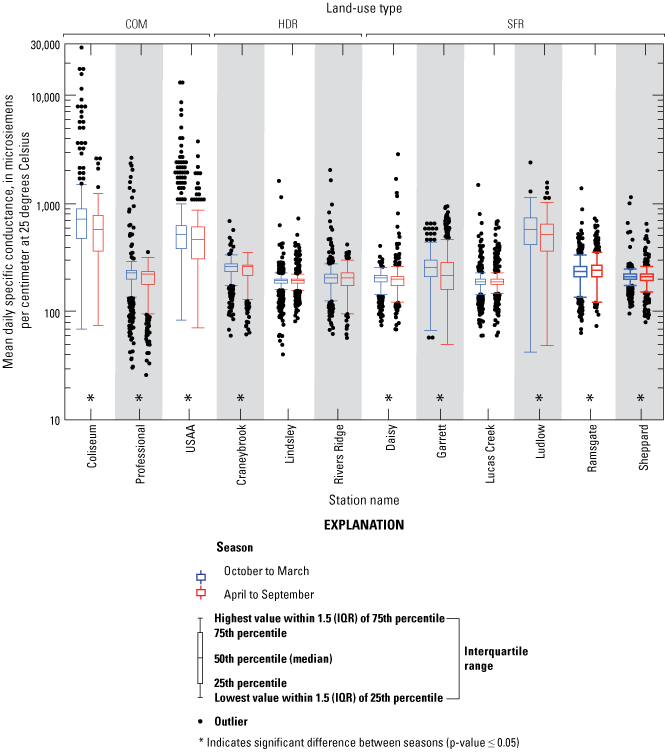
Mean daily specific conductance computed from continuous (5-minute interval) measurements at the 12 monitoring stations for water years 2016 through 2020, comparing data collected during the cool (October–March) and warm (April–September) seasons. A water year begins October 1 and ends September 30 of the following year. Station names and land-use types are defined in table 1.
Specific conductance of streamwater was significantly higher in cool months at 8 of the 12 stations and higher in warm months at Ramsgate. Elevated SC in cool months may suggest a seasonal effect resulting from the application and subsequent wash off of de-icer and anti-icer salts. At all stations, spikes in SC values often coincided with observed or forecast winter-weather (snow, sleet, ice; National Oceanic and Atmospheric Administration, 2022b), and typically were more than an order of magnitude higher than baseline SC values. Winter-weather storms are less common in Hampton Roads than in the northern and western regions of Virginia (National Oceanic and Atmospheric Administration, 2022b); however, even infrequent applications of anti-icer and de-icer salts can alter surface and groundwater chemistry (Kaushal and others, 2021). The ionic properties of these salts favor retention in soils and shallow groundwater and slow release over decades (Robinson and others, 2017). Furthermore, Cl- retention capacity is highest in sandy soils with high organic matter content, which are common characteristics of Coastal Plain PP soils (Robinson and others, 2017). Higher SC in cool months may be related to seasonally elevated base flows, which act to resuspend salts applied in previous winters, and can elevate SC even in years when de-icing salts are scantly applied.
Total Suspended Solids and Turbidity
Excess suspended sediment is a leading cause of water-quality and ecosystem impairment in urban streams. Although sediment transport occurs naturally and is controlled by fluctuations in streamflow, anthropogenic alterations like land development and stream channelization can increase erosional rates, decrease sediment transport time to streams, and increase the magnitude and recurrence of peak flows (Paul and Meyer, 2001; Soulsby and others, 2006). Suspended fine sediments, which account for 90 percent of the annual sediment load to Chesapeake Bay (Zhang and Blomquist, 2018), can serve as vectors by which contaminants are transported downstream (U.S. Environmental Protection Agency, 2000a). For example, sediment transported to Chesapeake Bay carries 77 and 18 percent of annual loads of TP and TN, respectively, and also conveys metals, pesticides, poly-chlorinated biphenyls, and other organic contaminants (Zhang and others, 2015). The average concentration of P and N on suspended-sediment particles in the Chesapeake Bay watershed is 1.0 milligram of phosphorus per gram and 3.6 milligrams of nitrogen per gram, respectively (Zhang and others, 2018). Additionally, fine sediments reduce light availability, causing reductions in photosynthesis and primary production (Wood, 1997), and, when deposited, can harm aquatic organisms (Luedtke and Brusven, 1976; Poulton and others, 2007; Rasmussen and others, 2009b).
Previous studies have reported higher concentrations of suspended sediment, suspended solids, and turbidity in urban watersheds than in agricultural or forested watersheds (Coulter and others, 2004; Ghane and others, 2016). Agricultural lands are more widespread than urban lands in the Chesapeake Bay watershed and account for 69 percent of the suspended sediment load to Chesapeake Bay (Brakebill and others, 2010; Langland and Cronin, 2003). The average sediment yield from urban lands, however, is approximately 6-times greater than forested yields and 3-times greater than yields from agricultural lands (Russell and others, 2017). Sediment loads typically are greater in rapidly urbanizing areas with active construction involving the removal of vegetation and excavation of soils than in older, previously developed urban regions (Carpenter and others, 1998; Langland and Cronin, 2003; Lee and Ziegler, 2010). In established, more stable impervious areas, common sources of suspended sediment and other suspended solids are dry and wet atmospheric deposition, erosion of the built environment (buildings and public infrastructure), and deterioration of vehicle parts and by-products. Soil erosion from pervious areas, especially poorly maintained lots, also contributes to the sediment load. Most of these solids are mobilized by overland runoff. These source pools are inherently limited in highly impervious landscapes; therefore, heavy rainfall events can temporarily deplete the sediment “reservoirs,” resulting in lower yields from successive storms (Lee and Ziegler, 2010).
Turbidity (TB) is a measure of the relative clarity of a body of water and typically has a strong relation with the concentration of total suspended solids (TSS; Swenson and Baldwin, 1965). Unlike TSS concentration, however, TB can be measured continuously and often can be used to estimate TSS concentration and load more accurately than models that include only a streamflow term (Jastram and others, 2009; Rasmussen and others, 2009a). In this study, the concentration of TSS was used in lieu of suspended-sediment concentration because TSS is the analytical metric used by the U.S. Environmental Protection Agency (EPA) for the Chesapeake Bay TMDL; however, it has been well established that the TSS method can result in the underestimation of suspended-sediment concentration (Galloway and others, 2005; Gray and others, 2000; Rasmussen and others, 2009a). This bias is particularly evident when sand constitutes more than 20 percent of a sample, which may be the case in Coastal Plain PP watersheds. Sand accounts for an average of 15 to 52 percent of the samples collected at four CB-NTN stations in the Virginia Coastal Plain PP (U.S. Geological Survey, 2022).
Concentrations of TSS in monthly samples, which most commonly represent base-flow conditions, generally were low (network median = 4.7 mg/L) but were substantially higher in samples collected during stormflow conditions (network median = 41.2 mg/L; app. 1, table 1.4). Total suspended solids concentration typically increased with streamflow at all stations (r = 0.631, p < 0.001; app. 1, table 1.5). At each station, a representative range of concentrations was sampled to allow for more accurate calculation of TSS loads. Median TSS concentrations were highest at Daisy (72.5 mg/L) and lowest at Ludlow (14.8 mg/L), both of which drain SFR watersheds (fig. 14). TSS concentrations were significantly higher in SFR watersheds than in HDR watersheds; concentrations were lower in COM watersheds than in both residential land-use types.
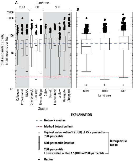
A, Total suspended solids concentrations at the 12 monitoring stations and B, variations in the concentrations across 3 land- use types for water years 2016 through 2020. A water year begins October 1 and ends September 30. Non-matching letters note statistically significant differences based on p less than or equal to 0.05. Station names and land-use types are defined in table 1.
The median TSS concentration across all samples (34.0 mg/L) was similar to NSQD data collected in Hampton Roads (41.0 mg/L) and lower than the nationwide median (56.0 mg/L; app. 1, table 1.6). Concentrations reported in the NSQD were subset to reflect only residential and COM land-use types to provide a direct comparison to data collected for this study. Total suspended solids concentrations did not differ significantly between residential and COM land-use types in the NSQD; however, more generally, land use was reported as a significant factor affecting TSS (Pitt and others, 2018).
Runoff on the rising limb of a storm hydrograph often is more contaminated than the water on the recession limb. Differences result from factors such as mobilization of anthropogenic contaminants, such as excess sediment and nutrients accumulated on the land surface during the antecedent dry weather period, and the rapid transport of precipitation runoff to the storm conveyance. Whether TB peaks before or after peak streamflow can inform the source and supply of TSS or other particulate-dominant constituents in the watershed and may provide insight for how best to implement BMPs to achieve reductions in load. The timing of peak TB on a hydrograph typically is identified through analyses of TB-streamflow hysteresis patterns; however, this method is best used to investigate single storm events rather than to characterize conditions across tens to hundreds of storms. Cross-correlation analyses, which considered data from approximately 200 to 500 storm events at each station, revealed TB peaks within 1 hour of peak streamflow in 87 percent of storms, indicating that the transport of particulate material is strongly correlated to increasing streamflow (fig. 15). At all stations, TB typically peaked before streamflow, which indicates disproportionate loading during the rising limb of the storm—a first flush. The concentration-based first-flush criterion has been previously defined by high initial concentration in the early part of a rainfall-runoff event, with a subsequent rapid concentration decline (Gupta and Saul, 1996; Sansalone and Cristina, 2004). Although lags were less than one hour for most storms, some events had strong positive lags of more than one hour (12 percent), indicating TB peaked well before peak streamflow and declined as the event progressed. This pattern suggests TSS were delivered quickly to the storm conveyances from storages within the pipe network, likely those sediments deposited by previous events, and accretion on impervious surfaces (Landers and Sturm, 2013).
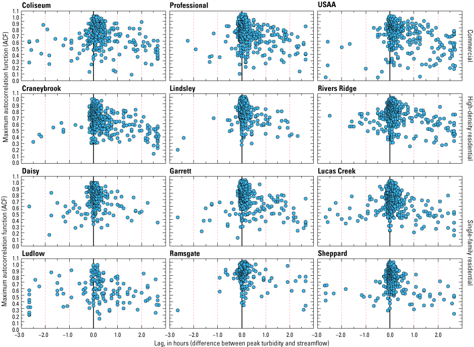
Cross-correlation analysis of turbidity concentration and streamflow. Positive lag values on the x-axis indicate that peak turbidity preceded peak streamflow, whereas negative values indicate that peak streamflow preceded peak turbidity. Each lag unit represents a one-hour difference between peak turbidity and streamflow. The strength of the relation between turbidity and streamflow is represented by the correlation function on the y-axis (1 equals perfect correlation, 0 equals no correlation). Station names are defined in table 1.
Cross-correlation analyses provide visual evidence of a first flush during some storm events, and mass-volume (M[V]) plots were used to quantify the occurrence of this phenomenon based on published criteria. The average maximum difference (ΔMax) in the cumulative TSS load and cumulative stormflow volume ranged from 0.20 to 0.31 at 10 of the 12 stations, exceeding Geiger’s (1987) 0.20 first-flush threshold; only the stations Daisy (0.18) and Ludlow (0.14) were below this level (table 5). Incorporating Gupta and Saul’s (1996) time term revealed that across the network, an average ΔMax of 0.23 occurred in the first 14 percent of the storm duration (which represents the first 1.21 hours of the average storm), conveying 68 percent of the TSS load in just 45 percent of the stormflow volume. The range of values across stations was minimal. The strongest average first flush occurred at Ramsgate, where ΔMax equaled 0.31 and occurred in the first 8.8 percent of the storm event, conveying 73 percent of the TSS load in just 42 percent of the stormflow volume. The weakest first-flush statistics were observed at Ludlow, where ΔMax occurred in the first 16 percent of the storm event, conveying 63 percent of the TSS load in the first 50 percent of the stormflow volume. Median ΔMax exceeded the 0.2 threshold at most stations and typically occurred in the first 20 percent of the storm duration, but there was considerable inter-storm variability (fig. 16). Variability between storm events was likely because of differences in rainfall volume and intensity, the antecedent dry weather period, and the accumulated mass of solids across the watershed and within the storm conveyance system (Bertrand-Krajewski and others, 1998; Vaze and Chiew, 2002). Given such variance, the prevalence and importance of the first-flush phenomenon is better investigated by computing the frequency of storms that exceed the 0.2 threshold. This threshold was exceeded in more than 50 percent of storms at 6 of the stations and ranged from 77 percent of the time at USAA to only 22 percent of the time at Ludlow (table 5, fig. 17). Generally, the strength of the first flush is proportional to degree of impervious cover, and inversely related to watershed size (Li and others, 2007; Ma and others, 2002). Delta-max scores were highest in COM watersheds, but scores for the two residential type watersheds were not significantly different from one another. Across the three land-use types there exists an increasing impervious gradient from COM to SFR and inverse relation with respect to watershed size; however, correlations between ΔMax and both impervious cover (r = 0.07; p = 0.829) and watershed area (r = -0.15; p = 0.649) were weak and non-significant.
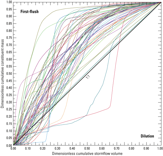
Set of mass-volume curves for total suspended solids at the Ramsgate station. Each line represents a single storm event. The 1:1 line indicates that mass transport is constant throughout the storm event.
Table 5.
Summary of mean total suspended solids mass-volume (M[V]) curves.[Unit values of streamflow and estimations of TSS for each extracted storm event are available in the associated data release (Porter, 2022). Station names and land-use types are defined in table 1. All monitoring stations, unless otherwise stated, are at storm drains. ΔMax, delta maximum; %, percent]
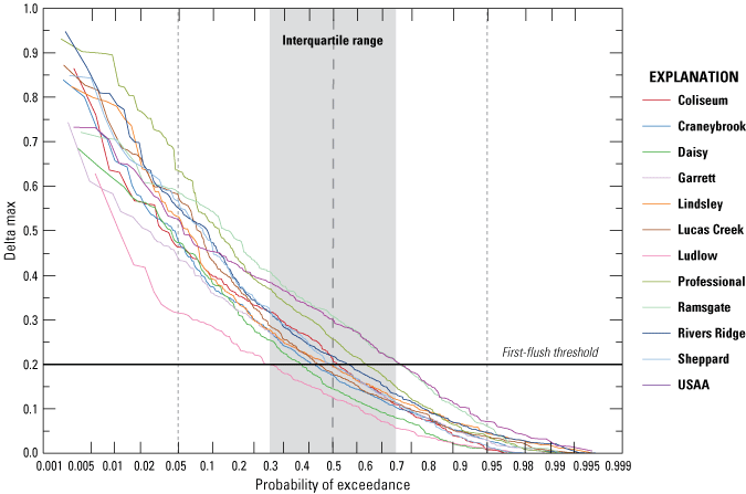
Frequency distribution of delta maximum for total suspended solids at each monitoring station. Values greater than 0.2 indicate a first flush based on criteria defined by Geiger (1987).
Previous studies also have used M(V) curves to suggest a first flush based on the percentage of the load conveyed by a given initial percentage of the stormflow volume; however, the criteria used to define this effect varies widely. For example, Wanielista and Yousel (1993) defined a first flush when 50 percent of the pollutant mass was transported in the first 25 percent of the volume. Bertrand-Krajewski and others (1998) employed a stricter criterion of at least 80 percent of the pollutant mass in the first 30 percent of stormflow volume, whereas Geiger (1987) defined the phenomenon as occurring when the mass ratio exceeds the stormflow volume ratio at all instances through an event. Regardless of the criterion used to define this phenomenon, this analysis describes the volume of stormflow that must be treated to reduce a given percentage of the load. In this study, station averages ranged from 60 to 75 percent TSS mass transport in the first 50 percent of stormflow volume, which when evaluated, along with ΔMax values and cross-correlation, results suggest the first flush is an important factor affecting TSS loadings during runoff events in these watersheds.
At all 12 stations, TB and streamflow were strong predictors of TSS concentration and load and explained, on average, greater than 90 percent of variability in load models and 80 percent of variability in concentration models (app. 1, table 1.7). Models typically were positively biased; however, the magnitude of bias was low—6 percent on average across the 12 station-specific models—and had high efficiency scores (average Nash-Sutcliffe efficiency = 0.72), suggesting accurate predictions of TSS loads at all stations. Half of the models included a base-flow term to adjust the y-intercept for differences in low-flow versus high-flow sample populations, and similarly a base-flow-by-TB interactive term to adjust the slope of the concentration-TB relation. At stations USAA, Daisy, and Ludlow, either water temperature or a seasonal term was fit, suggesting seasonal differences in the source of TSS inputs that alter the TSS-TB relation. Model coefficients and unit-value estimates of load and yield have been published (Porter, 2022).
Over the study period, median annual yields of TSS were highest at Professional (764 pounds per acre [lbs/acre]) and Coliseum (701 lbs/acre), two COM watersheds; the lowest yields occurred at Garrett (135 lbs/acre) and Ludlow (138 lbs/acre), two SFR watersheds (fig. 18; table 6). The average annual yield across all stations was 347 lbs/acre. In contrast to TSS concentrations, COM watersheds had on average higher TSS yields than the two residential land-use types. The seemingly contradictory relation between concentration and yield results from elevated streamflow yields generated in the COM watersheds, which transport a greater mass of TSS, albeit at a lower concentration. Across all stations, an average 88 percent of TSS loads was conveyed by stormflows (fig. 19). In past studies, both runoff volume and constituent transport have been well correlated with urban factors, such as total impervious area, effective impervious area (impervious areas connected directly to stormwater inlets), and road density (Hatt and others, 2004; Janke and others, 2017; Walsh and others, 2005b). Annual TSS yield was moderately correlated with annual streamflow yield and may reflect limited pools of available sediment in these watersheds that are typically exhausted in the early phase of a storm, regardless of magnitude or duration (fig. 2.1A).
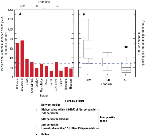
A, Bar plot of median annual total suspended solids yield at the 12 monitoring stations and B, boxplots of annual total suspended solids grouped by land use for water years 2016 through 2020. Non-matching letters denote statistical significance based on p less than or equal to 0.05. A water year begins October 1 and ends September 30. Station names defined in table 1.
Table 6.
Summary of annual total suspended solids loads and yields at each monitoring station for water years 2016 through 2020.[Station names and land-use types are defined in table 1. All monitoring stations, unless otherwise stated, are at storm drains. A water year begins October 1 and ends September 30 of the following year. TSS, total suspended solids; NA, not applicable]
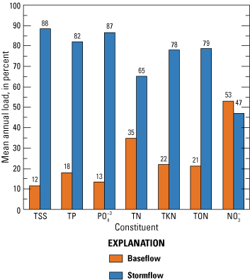
Bar plot showing the proportion of the mean annual load of total suspended solids across the 12 monitoring stations for water years 2016 through 2020 delivered during periods of stormflow and base-flow conditions. Numbers inset in bars indicate the percentage of the total load. A water year begins October 1 and ends September 30.
Comparison of sediment yields (in terms of either TSS or suspended sediment concentration) from Hampton Roads, Fairfax County (Porter and others, 2020), the CB-NTN (Moyer and Langland, 2020), and Gwinnett County, Georgia (Aulenbach and others, 2017) reflect key factors affecting sediment transport such as watershed size, land development, physiographic province, and differences in earthen streams versus engineered concrete stormwater conveyances. Headwater streams typically transport more sediment than higher-order streams owing to a lack of opportunity for in-channel deposition and greater energy availability for entrainment (Smith and Wilcock, 2015), and sediment yields typically are higher in developed watersheds than in forested or agricultural watersheds (Brakebill and others 2010). The Hampton Roads watersheds are an order of magnitude smaller and substantially more developed (high percent of impervious cover) than those draining the monitored Fairfax County streams, yet sediment yields were 2 to 3.5 times lower at Hampton Roads (fig. 20).
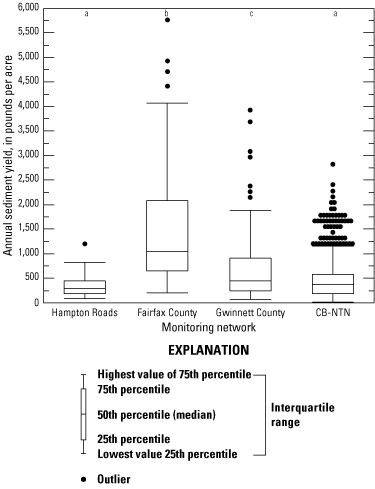
Sediment yields from watersheds in four monitoring networks—Hampton Roads, Fairfax County, Virginia, Gwinnett County, Georgia, and the Chesapeake Bay Non-tidal Network (CB-NTN). Non-matching letters denote statistical significance based on p less than or equal to 0.05. Sediment is quantified as total suspended solids (TSS) for Hampton Roads and Gwinnett County, whereas values for Fairfax County and the CB-NTN represent suspended sediment.
Low TSS yields in Hampton Roads watersheds may result from a lack of bank erosion, a sediment source which is absent in concrete pipes and conveyance channels. Yields also may differ between comparison networks because of unique characteristics of each physiographic province. Higher yields in the Piedmont PP have been linked to available pools of legacy sediment and high rates of soil erosion, whereas very little fine-grained sediment is transported from the characteristically sandy streams of the Coastal Plain PP (Gellis and others, 2009). In fact, from 1952 through 2001, the average annual sediment yield of Coastal Plain PP streams (106 pounds per acre per year [lbs/acre/yr]) was nearly 10 times lower than that of Piedmont PP streams (925 lbs/acre/yr), and nearly 6 times lower than streams in the Appalachian Plateaus, Blue Ridge, and Valley and Ridge PPs (Gellis and others, 2009). Coastal Plain PP streams have been described as “bottle-necks” (Phillips and Lutz, 2008) that are created by a transition from narrow, high-energy bedrock streams in the Piedmont PP to low-energy systems with broad alluvial floodplains. These latter streams have high rates of inundation and sediment attenuation and limit delivery of sediment to Chesapeake Bay (Noe and Hupp, 2009; Ensign and others, 2015). Although TSS yields from streams in the study watersheds in the Coastal Plain PP were low relative to yields from monitored urban streams in other physiographic provinces, previous research has reported a tenfold decrease in rates of sediment trapping in urbanized Coastal Plain PP streams that, like those in this study, have been artificially channelized and consequently disconnected from surrounding floodplains (Noe and Hupp, 2009). Hampton Roads watersheds are several orders of magnitude smaller and far more developed than most CB-NTN streams, but yields did not differ significantly. That yields did not differ, despite watershed size, channelization, and high levels of imperviousness, the similarity in yields suggests a lack of available substrate and mechanism for TSS entrainment in urban Coastal Plain PP watersheds.
Phosphorus
Phosphorus is an essential nutrient for the growth of plants and animals but excess P in aquatic ecosystems can lead to eutrophication and, in turn, to ecosystem degradation. Phosphorus readily binds to soils and fluvial sediment, and therefore generally enters surface waters via overland flow rather than as inflow of groundwater. Phosphorus commonly is associated with erosional processes and transported downstream via suspended solids (Correll, 1998; Denver and others, 2010); however, these matrices have a finite capacity to sorb P (Richardson and Craft, 1993). When this capacity is met, referred to as P saturation, the unsorbed P fractions may be exported to streams as dissolved P (primarily in the form of orthophosphate), and can result in degraded aquatic ecosystems (Conley and others, 2009), as this is the preferred form for uptake by aquatic organisms. Further, the release of P from particulates can be catalyzed by warmer temperatures (Duan and Kaushal, 2013), anoxia (House and Denison, 2002; Lehtoranta and Pitkänen, 2003), anthropogenic inputs (Sharpley, 1995), increases in pH (James and Barko, 2004), and changing salinity levels (Haq and others, 2018). For example, warmer temperatures stimulate microbial degradation of the organic material to which the P was previously sorbed (Duan and Kaushal, 2013). In oxic environments, P bonds to organic matter and to clays containing iron (Fe) and aluminum (Al) oxides and may remain stored in streambank and streambed sediments (Fink and others, 2016; Lehtoranta and Pitkänen, 2003; Manning and Wang, 1994). Under reduced oxygen conditions, however, those bonds can weaken, resulting in diffusion of dissolved P to the water column (Correll, 1998). Additionally, as pH increases, P is liberated from Fe and Al oxides because of competition with hydroxide ions (Fink and others, 2016). Freshwater salinization also may increase P concentrations in streams through competition for binding sites on soil particles with negatively charged ions in the saline water (Bruland and DeMent, 2009).
In undeveloped watersheds, phosphorus bound to soils is mostly immobile; in urban systems, however, overland flow across impervious surfaces can mobilize and transport sediments and plant material to storm drains and the downstream receiving body. As a result, transport of P typically is higher in urban than in undeveloped watersheds (Alvarez-Cobelas and others, 2009; Duan and others, 2012; Meybeck, 1998). Urbanization has been associated with a shift in P transport from low to high streamflow conditions that result from greater runoff volume and increased sediment mobilization (Duan and others, 2012). Common sources of phosphorus in urban watersheds include fertilizer (applied to lawns), geologically derived P, animal or pet waste, decomposition of plant and animal matter, road salt, and point-source discharges of wastewater (LaValle, 1975; Paul and Meyer, 2001). There are no permitted point-source discharges of wastewater into the monitored Hampton Roads watersheds, highlighting the importance of understanding of non-point source inputs. Turf grass and roadways typically account for most of the P in urban runoff. Grass clippings, leaf litter, and fertilizer are the predominant sources in residential areas, whereas runoff from roadways is a bigger contributor in COM and industrial watersheds (Waschbusch and others, 1999). Orthophosphate stored in sediment pore water also can be remobilized to streams and storm conveyance systems during high-runoff events (Duan and others, 2012). A phosphorus criterion specific to Virginia streams currently does not exist; however, the EPA reference condition for streams in Hampton Roads (ecoregion 63) is 0.05 mg/L (U.S. Environmental Protection Agency, 2000b).
Concentrations of total phosphorus and PO43- in monthly samples, which typically represent base-flow conditions, were generally low (network median TP = 0.06 mg/L; PO43- = 0.01 mg/L; app. 1, table 1.4) but substantially higher in samples collected during stormflow conditions (network median TP = 0.24 mg/L; PO43- = 0.08 mg/L). In stormflow samples, median TP concentrations were highest at Daisy (0.39 mg/L) and lowest at Professional (0.07 mg/L). Concentrations of TP were higher in SFR watersheds than in HDR watersheds; concentrations at COM were lower than in both residential types (fig. 21). This pattern may reflect differences in the type or quantity of P inputs in these watersheds or may reflect greater dilution across the impervious gradient—a function of differences in stormflow yields. A likely source of P in these watersheds is the flushing of solids accumulated on impervious surfaces during the period between storm events. Inputs of P sources such as grass clippings, leaf litter, and pet waste are likely more abundant in residential than COM areas because of differences in land-cover attributes and human activities. In a previous study, TP concentration in street accumulations was 29 percent greater in residential watersheds than in COM watersheds and accumulated at five times the rate in the former type of watersheds (Sorenson, 2013). Concentration increased with streamflow at most stations (r = 0.424, p < 0.001); however, this relation was slightly negative at Ludlow and weak at the other stations that experience backwater during periods of high flow or high tide (Professional, Coliseum, USAA, and Sheppard; app. 1, table 1.5). Backwater conditions may affect concentration of P by dilution or enhanced settling of particulates because of low water velocity; however, particulates that become disentrained are likely remobilized on the rising limb of the succeeding storm.
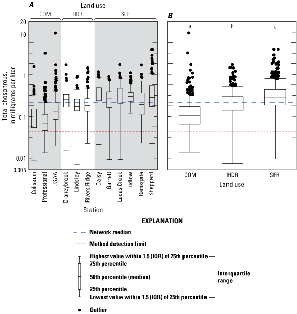
A, Concentrations of total phosphorus at the 12 monitoring stations and B, across 3 land-use types for water years 2016 through 2020. A water year begins October 1 and ends September 30. Non-matching letters note statistically significant differences based on p less than or equal to 0.05. Station names and land use types are defined in table 1.
The median TP concentration across all network samples (0.22 mg/L) was lower than NSQD stations located in residential and COM land uses (0.27 mg/L) and the subset of those stations in Hampton Roads (0.27 mg/L; app. 1, table 1.6). Likewise, the median PO43- concentration in samples collected in this study (0.07 mg/L) was less than half the nationwide average reported in the NSQD (0.16 mg/L). The results for orthophosphate analyses were not available for the subset of NSQD stations in Hampton Roads, though the median dissolved phosphorus concentration (0.14 mg/L) was double that in the study watersheds. Similar to this study, the NSQD reports a significantly higher concentration of TP and dissolved P in residential than COM land uses.
The concentration and composition of TP varied both spatially and seasonally. Concentrations of PO43- and the remaining portion of TP, defined as total particulate P plus dissolved organic P, were inversely related to the development gradient in the three land-use types: COM < HDR < SFR (fig. 22). Orthophosphate accounted for a significantly smaller proportion of TP in COM watersheds than in the two residential types, suggesting spatial variability in sources of P across land-use types. Seasonal shifts in composition indicate variability in sources throughout the year. Orthophosphate concentrations increased in summer and fall, and declined sharply in winter and spring, whereas the particulate plus organic fraction was highest in winter and spring (app. 1, table 1.8). Elevated PO43- concentrations in summer months may be related to high rates of microbial degradation of organic matter and diffusion of P from soils and metal oxides. Additionally, annual P loadings from unbagged grass clippings left on nearby impervious surfaces such as sidewalks and curbs can be substantial, ranging from 0.35 to 6.69 lbs/acre (Soldat and Petrovic, 2008). In fall months, leaf senescence can contribute substantial inputs of organic detritus to storm conveyance systems and has been linked to high concentrations of in-stream dissolved P (Janke and others, 2017; Kluesener and Lee, 1974; Selbig, 2016). Most of the phosphorus contained in leaf litter can dissimilate in the first 24 to 48 hours of soaking (Hobbie and others, 2014; Wallace and others, 2008). In a study of urban stormwater in Madison, Wisconsin, 56 percent of the annual TP yield was related to leaf litter in the fall, compared to only 16 percent in study areas where leaf removal was implemented, and most of the P was in the dissolved form – 85 percent in fall versus less than 50 percent in spring (Selbig, 2016). Likewise, Janke and others (2017) report a strong correlation between urban tree canopy and P loads (r = 0.84). Lawn fertilizer containing P most commonly is applied in fall months during establishment or overseeding of cool-season grasses, as allowed under the current restrictions on P in fertilizers in Virginia (VA Code 3.2-3600 and 10.1-104.5). Simulations of runoff events immediately following fertilizer applications have shown substantial losses (<1 to 18 percent of the fertilizer applied), and in worst-case simulations contributed a year’s worth of P from a single event (Soldat and Petrovic, 2008). Higher amounts and concentrations of particulate P in winter and spring months may result from elevated streamflows capable of entraining P bound to sediments and organic matter as well as seasonally lower rates of P dissimilation.
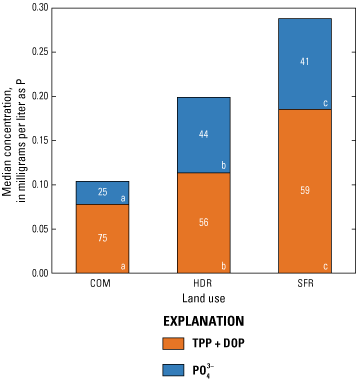
Median concentrations of phosphorus species in samples collected in water years 2016 through 2020 and grouped by land use. A water year begins October 1 and ends September 30. Statistical differences in total particulate phosphorus plus dissolved organic phosphorus (TPP + DOP) and PO43- between land-use types are noted with non-matching letters and is based on p less than or equal to 0.05. Numbers inset in bars are the median percent composition of total phosphorus. Land-use types are defined in table 1.
Total phosphorus concentrations peaked within one hour of peak streamflow in 83 percent of storms, indicating concentration is well correlated with streamflow (fig. 23). Positive lags greater than one hour were rare, though TP peaked before streamflow in 61 percent of storms. This pattern suggests a disproportionate mass of P typically was transported on the rising limb of the storm hydrograph. Median station ΔMax values were less than the 0.2 first flush threshold at all stations except Ramsgate (0.21), where this threshold was exceeded during 54 percent of storms (table 7; fig. 24). The threshold was exceeded in less than 50 percent of events at the other 11 stations. Although this strict criterion for a first flush was rarely met, M(V) curves confirm results of cross-correlation analyses that indicate biased loading towards the beginning phase of the runoff response. On average, approximately 60 percent of the TP load was transported by the first 46 percent of stormflow volume. Delta-max scores were highest in COM watersheds, but not statistically different between the two residential types of land uses. Phosphorus loadings typically are well correlated with TSS given an affinity to bind to sediments and organic matter. Differences in the frequency of the first flush phenomenon between these two constituents likely reflects contributions of dissolved P loadings and indicates differences in the source and timing of inputs. Storage of water-soluble P in the thin zone of surface soils and organic matter can desorb and enter waterways as bioavailable PO43- (Sharpley and others, 1981). Unlike with sediment wash off from impervious surfaces or resuspension of previously deposited particulates within the stormwater system, this process requires soil saturation, and consequently is less likely to occur during the initial flush of runoff.
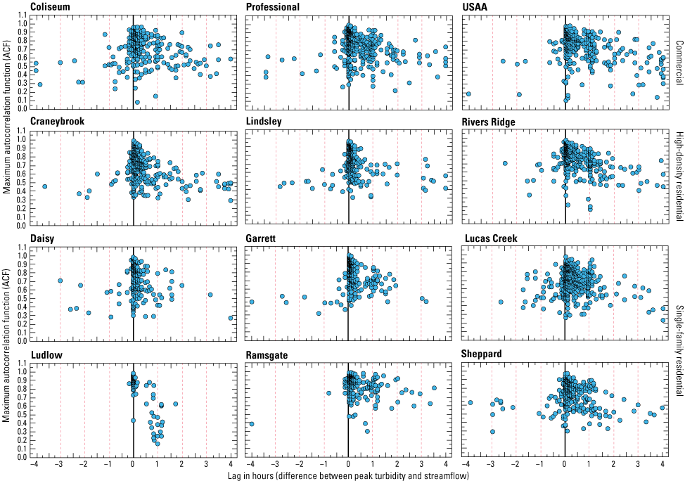
Cross-correlation analysis of total phosphorus (TP) concentration and streamflow. Positive lag values on the x-axis indicate that peak TP preceded peak streamflow, whereas negative values indicate that peak streamflow preceded peak TP. Each lag unit represents a 1-hour difference between peak TP and streamflow. The strength of the relation between TP and streamflow is represented by the correlation function on the y-axis (1 equals perfect correlation, 0 equals no correlation). Station names are defined in table 1.
Table 7.
Summary of mean total phosphorus mass-volume (M[V]) curves.[Unit values of streamflow and estimations of TP for each extracted storm event are available in the associated data release (Porter, 2022). Station names and land-use types are defined in table 1. All monitoring stations, unless otherwise stated, are at storm drains. ΔMax, delta maximum; %, percent]
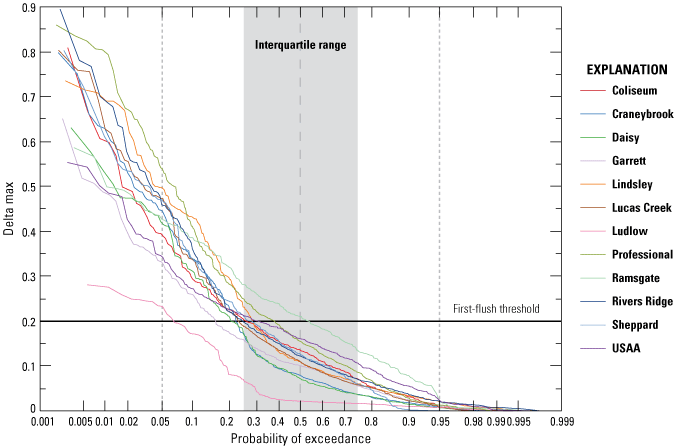
Frequency distribution of delta maximum for total phosphorus. Values greater than 0.2 indicate a first flush based on Geiger (1987).
Total phosphorous concentrations and loads generally were well predicted by models that contained turbidity and streamflow terms. Inclusion of these terms and the strength of their predictive power reflects the strong relation between sediment and phosphorous transport; on average, models explained 96 and 68 percent of variability in load and concentration, respectively (app. 1, table 1.9). On average, models were efficient (Nash-Sutcliffe efficiency = 0.82) and had low bias (2 percent), which indicates accurate predictions of TP loads. Half of the models included a base-flow term to adjust the y-intercept for differences in low-flow versus high-flow sample populations, which suggests differences in the source of P depending on hydrologic condition. Models for most stations included either water temperature or a seasonal term, indicating seasonal variance in P inputs that alter the TP-TB relation. Orthophosphate models had lower predictive power than TP models, explaining, on average, 92 and 49 percent of the variability in load and concentration, respectively (app. 1, table 1.10). Similar to findings in previous studies (Porter and others, 2020; Robertson and others, 2018), model bias in this study was higher in PO43- models (average 12 percent) and efficiency of predictions was lower (average Nash-Sutcliffe efficiency = 0.67); however, these diagnostics are within the range of acceptable results for use in load computation (Lorenz and others, 2015; Nash and Sutcliffe, 1970). Model coefficients and unit-value estimates of load and yield are published in Porter (2022).
Total phosphorus and PO43- yields varied across stations, though no significant effect of land use was observed for TP (fig. 25; app. 2, fig. 2.2). Over the study period, median annual TP yield was highest at Ludlow and USAA, and networkwide ranged from 0.62 to 2.39 lbs/acre. The average annual yield across all stations was 1.37 lbs/acre (table 8). The median annual PO43- yield at Lucas Creek and Ludlow were approximately double and triple the network median, respectively, and yields ranged from 0.12 to 1.57 lbs/acre networkwide (app. 1, table 1.11). Annual streamflow yield was moderately correlated with TP yield but poorly with PO43- (app. 2, fig. 2.1B and 2.1C). Nonetheless, TP and PO43- loads were transported predominantly during periods of stormflow (> 80 percent; fig. 19). This apparent contradiction suggests the recurrence of storms was a bigger driver of annual yield than the magnitude of those events or the volume of water exported from the watershed each year. The two most likely transport pathways of P during runoff events are erosion of sediment-bound P and dissolution of soluble P stored in soils and organic matter, both on the land surface and within the stormwater conveyance system. The portion of P transported during base flows is likely dominated by PO43- and dissolved organic P leached from inputs on the land surface to the underlying water table (Yang and Toor, 2018). When buried storm conveyance systems intercept the water table, these systems provide preferential flow paths (urban karst) as groundwater moves through leaks, cracks, and joints in the concrete infrastructure, and along the highly permeable gravel-filled trenches that commonly surround these systems (Bonneau and others, 2017; Kaushal and Belt, 2012; Sharp and others, 2003). The effect of urban karst is reduced attenuation and removal of phosphorus and other soluble constituents through biogeochemical cycling and sorption, leading to their increased transport.
Table 8.
Summary of annual total phosphorus loads and yields at each monitoring station for water years 2016 through 2020.[Station names and land-use types are defined in table 1. A water year begins October 1 and ends September 30. All monitoring stations, unless otherwise stated, are at storm drains. TP, total phosphorus; NA, not applicable]
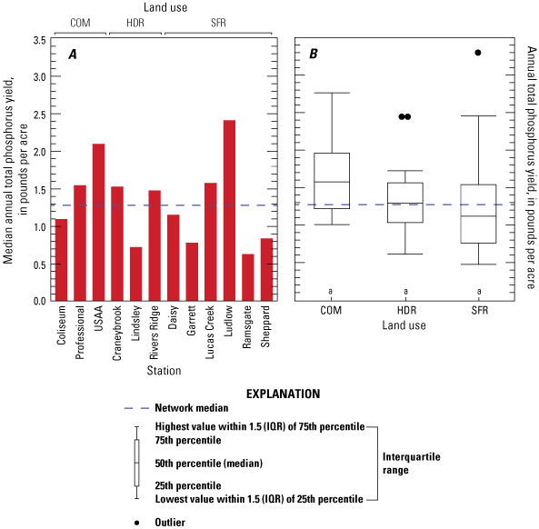
Total phosphorus yields presented as A, a bar plot of the median annual total from water year 2016 through 2020 at each of the 12 monitoring stations and B, boxplots of annual yields grouped by land use over the same period. A water year begins October 1 and ends September 30. Non-matching letters denote statistical significance based on p less than or equal to 0.05. Station names and land use acronyms defined in table 1.
Mean annual yields of TP and PO43- from the Hampton Roads study watersheds were higher than those documented in the monitoring networks in comparison studies (fig. 26) as well as estimations for other developed watersheds in the North Carolina-Virginia coastal region (Dodd and others, 1992; Lin, 2004). Previous studies of urban watersheds in Virginia linked high rates of TP transport to similarly high yields of suspended sediment (Jastram, 2014; Porter and others, 2020). The relatively low TSS yields reported in these 12 Hampton Roads watersheds indicate that non-sediment related sources of P, such as organic matter and PO43-, may dominate in this region. The primary driver of differences in TP yields between the Hampton Roads and Fairfax County networks was elevated levels of PO43-, rather than particulate P, in Hampton Roads. Yields in Hampton Roads may be intrinsically higher than those found in comparison studies because of factors related to scale—stream order and watershed size. Larger watersheds and higher-order streams typically have smaller sediment and nutrient yields than small headwater streams, as a result of fluvial trapping of sediments and those nutrients (Smith and Wilcock, 2015). Furthermore, P retention may be limited by the high drainage density of the Hampton Roads watersheds, which have been artificially expanded by the engineered stormwater network of ditches, concrete channels, and buried pipes.
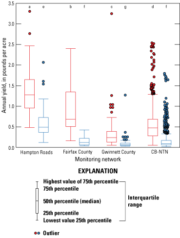
Boxplots of annual total phosphorus (red) and orthophosphate (blue) yields from four monitoring networks—Hampton Roads and Fairfax County, Virginia, Gwinnett County, Georgia, and the Chesapeake Bay Non-tidal Network (CB-NTN). Non-matching letters denote statistically significant differences based on p less than or equal to 0.05 in total phosphorus and orthophosphate between networks.
Phosphorus yields also may be elevated as a consequence of soil properties and geological features of the Coastal Plain PP. The degree of phosphorus retention in Coastal Plain PP soils ranges from low to moderate (USDA-NRCS, 1998) and is influenced by the P saturation level and soil texture. The Spatially Referenced Regression on Watershed attributes (SPARROW) model has similarly identified high rates of P transport in the Coastal Plain, and researchers have attributed this to soil saturation resulting from historical P applications (Ator and others, 2011). When soils become P saturated, retention is limited, and applied P may be readily lost through runoff and leaching. Retention also is influenced by soil texture; soils with high clay content have a greater P sorption capacity than do sandy soils, because of grain size and the net negative charge of the soils, which affects surface-area availability and the ability to form bonds with positively charged nutrients (Ballard and Fiskell, 1974; Olsen and Watanabe, 1957; Xu and others, 2006). Soils in the Coastal Plain PP are characteristically coarse-textured sands and silts, particularly in the upper soil horizons, as compared to the fine clays common throughout the Piedmont PP (Sanford and others, 2012; Thomas and Harper, 2009). Furthermore, Coastal Plain PP soils are more dominated by Al oxides than by Fe oxides, whereas the inverse is true of soils in the Ridge and Valley and the Piedmont PP (Penn and others, 2006). Previous studies have reported a negative correlation between dissolved P in runoff and the clay and Fe content of soils (Cox and Hendricks, 2000; Penn and others, 2006). This relation reflects the formation of stronger bonds between P ions and Fe oxides compared to those with Al oxides; therefore, Fe-associated P is less likely to desorb in runoff (Aura, 1978). Given these factors, Coastal Plain PP soils may have a greater potential to release dissolved phosphorus in runoff compared to the upland PPs of Virginia, given identical inputs of soluble P to the landscape (Penn and others, 2006).
In the Coastal Plain PP, the proximity of the surficial aquifer to the land surface, and water table that lies within it, makes it susceptible to contamination by anthropogenic inputs (McFarland and Bruce, 2006) and may promote lateral transport of dissolved P in runoff and groundwater discharging to streams and stormwater conveyances (Ballard and Fiskell, 1974; Harris and others, 1996). Elevated P yields also may be related to high organic matter content that is characteristic of the Coastal Plain PP, a product of the low topographic gradient and resulting low-velocity streams. Organic matter can affect available P in two ways: (1) microbial mineralization of organic materials such as plant debris and animal waste and the ensuing release of previously adsorbed P (Upreti and others, 2015); and (2) coating of sorption sites on metal oxides. Negatively charged substances in organic matter can interact with positively charged oxides, such as Al and Fe, creating competition for binding sites and consequently reducing the potential for P adsorption (Liu and others, 1999) and increasing desorption (Hinsinger and others, 2011).
Nitrogen
Nitrogen (N) is a naturally occurring element that is essential to the growth of plants and animals, but inputs of N exceeding ecosystem processing and storage capacities may be exported to downgradient waters (Hem, 1985; Paul and Meyer, 2001). Excess N can cause eutrophication, excessive algal growth, hypoxia, reduced water clarity, and harmful algal blooms, which degrade aquatic ecosystems and may pose risk to human health (Galloway and others, 2003; Hem, 1985; Hobbie and others, 2017). Common anthropogenic sources of N in the urban landscape include atmospheric deposition, lawn fertilizer, leaking wastewater infrastructure, septic systems, and pet waste (Bettez and Groffman, 2013; Hyer and others, 2016; Paul and Meyer, 2001); natural sources include plant decomposition and biological fixation (Carpenter and others, 1998; Wanielista and others, 1977). The export of N associated with these inputs is positively correlated with urban development (Shields and others, 2008; Tasdighi and others, 2017), though N retention varies with watershed size (Groffman and others, 2004).
Nitrogen loading in urban watersheds is composed of both inorganic (nitrate [NO3-], nitrite [NO2-], ammonia [NH3], and ammonium [NH4]) and organic (both dissolved and particulate) forms, though many studies report organic N as the primary component in urban runoff (Jani and others, 2020; Lusk and Toor, 2016; Seitzinger and others, 2002; Seitzinger and Sanders, 1997; Taylor and others, 2005). Leaf litter, grass clippings, and other organic detritus and particulate matter are the primary sources of organic N in urban watersheds (Bratt and others, 2017; Janke and others, 2017; Selbig, 2016). Organic N, previously considered largely biologically unavailable, has been reported in several recent studies to be a significant source of reactive N for the phytoplankton and cyanobacteria linked to water-quality impairment (Bratt and others, 2017; Jani and others, 2020; Petrone, 2010; Wiegner and others, 2006). Coastal Plain PP streams typically have elevated concentrations of dissolved organic N, a consequence of characteristically high rates of organic matter accumulation, but relatively low concentrations of dissolved inorganic N (Gold and others, 2019). In urban streams, inputs of dissolved inorganic N may be elevated by anthropogenic activities, and changes in watershed hydrology following urban development have been shown to increase loadings of all forms of N (Gold and others, 2019; Petrone, 2010). A nitrogen criterion specific to Virginia streams has not been established; however, the EPA reference condition for streams in Hampton Roads (ecoregion 63) is 0.87 mg/L for TN and 0.04 mg/L for NO3- (U.S. Environmental Protection Agency, 2000b).
The network median TN concentration in base-flow samples (1.28 mg/L) was similar to the median stormflow concentration (1.43 mg/L) but the concentration and composition of TN varied between stations (app. 1, table 1.4). Concentrations were highest at Lindsley (3.43 mg/L) and Lucas Creek (3.93 mg/L), but typically were low (approximately 0.80 mg/L) at the three COM stations. Spatial variance in TN was moderated during stormflows (range = 1.07 mg/L), reflecting low inter-station variability of NO3- and TON in runoff, and highlighting the occurrence of NO3- in groundwater discharges as an important driver of overall differences between stations. The network median NO3- concentration of 0.46 mg/L in base-flow samples was similar to the median concentration in the surficial aquifer of the Coastal Plain PP (0.2 mg/L), reported by McFarland (2010). Some wells sampled by McFarland (2010) that were located on agricultural lands exceeded 10 mg/L of NO3-; however, most of the 482 wells measured were less than 1 mg/L, similar to the monitored Hampton Roads stormwater conveyances.
Concentrations of total N varied significantly across the three land-use types—highest in SFR watersheds and lowest in COM watersheds (fig. 27). This pattern may reflect differences in the type or quantity of N inputs across these land-use types or greater dilution across the impervious gradient, a function of differences in stormflow yields. The median TN concentration for the 12 study watersheds (1.41 mg/L) was lower than that for NSQD residential and COM stations (2.63 mg/L); TN concentrations were not available for the subset of NSQD stations within the Hampton Roads study area. Likewise, mean TKN and NO3- concentrations in samples collected in this study were lower than those in NSQD data collected in the Hampton Roads area and nationwide (app. 1, table 1.6). Similar to values from this study, TN, TKN and NO3- concentrations in the NSQD were higher in watersheds draining residential than COM land uses.
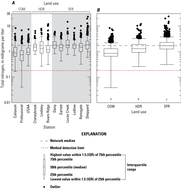
A, Total nitrogen concentrations at the 12 monitoring stations and B, across 3 land-use types for water years 2016 through 2020. A water year begins October 1 and ends September 30. Non-matching letters indicate statistically significant differences in concentration between land-use types. Significance is based on p less than or equal to 0.05. Station names and land-use types are defined in table 1.
Total nitrogen was composed of approximately 70 percent TON, 20 percent NO3-, and 10 percent NH3 across all three land-use types. Concentrations of NO3- and NH3 were lowest in COM watersheds, and TON concentrations varied across the full land-use gradient (fig. 28). Composition of TN also varied with hydrologic conditions; during base flow, TON constituted only 29 percent of TN but became 69 percent of TN during stormflow. In contrast, NO3- accounted for 57 percent of TN in base flow and only 15 percent in stormflow. This compositional shift signals a change in the source of N from NO3--enriched groundwater discharges during dry weather periods to TON dominant runoff during storm events. On average, TN was not well correlated with streamflow (r = -0.002, p < 0.921), a consequence of the contrasting positive relation to TON and negative relation to NO3- that cancel out when aggregated as TN. In most watersheds, which were more strongly dominated by TON, weak but significant positive correlations exist (app. 1, table 1.5). Conversely, at Lucas Creek and Lindsley, where NO3- is the dominant form of nitrogen, the negative relation suggests dilution with increasing streamflow.
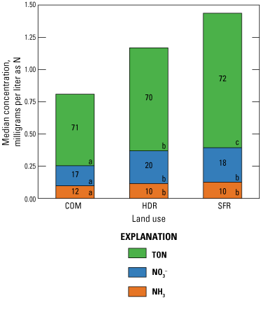
Median concentrations of total nitrogen (full bar), total organic nitrogen (TON), nitrate plus nitrite (NO3-), and ammonia plus ammonium (NH3) in samples collected in water years 2016 through 2020 and grouped by land use. A water year begins October 1 and ends September 30. Statistical differences in TON, NO3- and NH3 between land-use types are noted with non-matching letters. Numbers inset in bars are the median percent composition of total nitrogen. Land-use types are defined in table 1.
The concentrations of the different forms of nitrogen varied seasonally, with the highest concentrations of TN in the spring, driven primarily by seasonal fluctuations in TON (app. 1, table 1.12). Organic N typically is bound to sediments and organic matter; therefore, elevated concentrations in springtime may be related to similarly high concentrations of TSS. Seasonal differences in NO3- were minimal and suggest year-round contributions from one or more sources, or low denitrification potential in local soils. Terrestrial denitrification (reduction of NO3– to atmospheric N2) often is the dominant nitrogen loss term in N budgets of mid-Atlantic watersheds (Van Breemen and others, 2002), and typically results in greater NO3– loss in warmer months because of increased heterotrophic respiration (Deek and others, 2010; Meng and others, 2018; Porter and others, 2020; Tufford and others, 1998). Rates of NO3- loss vary in the Coastal Plain PP as a result of heterogenous lithology but are low in watersheds with predominantly sandy sediments where water remains oxic (Ator and others, 2011; Ator and Denver, 2015). Further, concrete stormwater infrastructure largely disconnects streamflow from the hyporheic zone, where microbial mediated processes such as denitrification occur (Merill and Tonjes, 2014). Denitrification potential was not measured as part of this study but may be a relevant factor driving the lack of a seasonal variation in NO3- concentrations across the network. The lack of seasonality in NO3- may also be related to the absence of periphyton and other algae in these stormwater systems. In natural streams, these organisms play an important role in improving water quality by temporarily sequestering N and P during periods of high growth, but owing to a lack of sunlight, are unlikely to thrive in subterranean stormwater pipes (Santhana Kumar and others, 2017).
Concentrations of TN typically peaked within one hour of peak streamflow (77 percent of storms; fig. 29). The timing of peak concentration reflects the dominant particulate composition of TN in stormflows and suggests that N transport may occur via similar pathways as do TSS and TP during periods of runoff. Total N peaked before streamflow in 72 percent of storms, suggesting a disproportionate mass of TN typically is transported on the rising limb of the storm hydrograph. This occurs from either the remobilization of deposits within the storm conveyance system or from sources nearby or directly connected to sewer inlets. Longer positive lags occurred in COM and HDR than in SFR watersheds, which may result from differences in the areal coverage and connectivity of impervious surfaces to stormwater infrastructure. These landscape features typically promote a more rapid first flush of constituent loadings to the stormwater conveyance system because of the directness of the flow path (Li and others, 2007). Exceptions were observed at Lucas Creek and Lindsley, where a negative lag occurred (TN peaked after streamflow) in more than 20 percent of storm events. Base-flow NO3- was substantially higher in these two watersheds, and a pattern of negative lags suggests (1) delayed contributions of NO3- from groundwater or interflow; or (2) transport of N sources farther from the monitoring station.
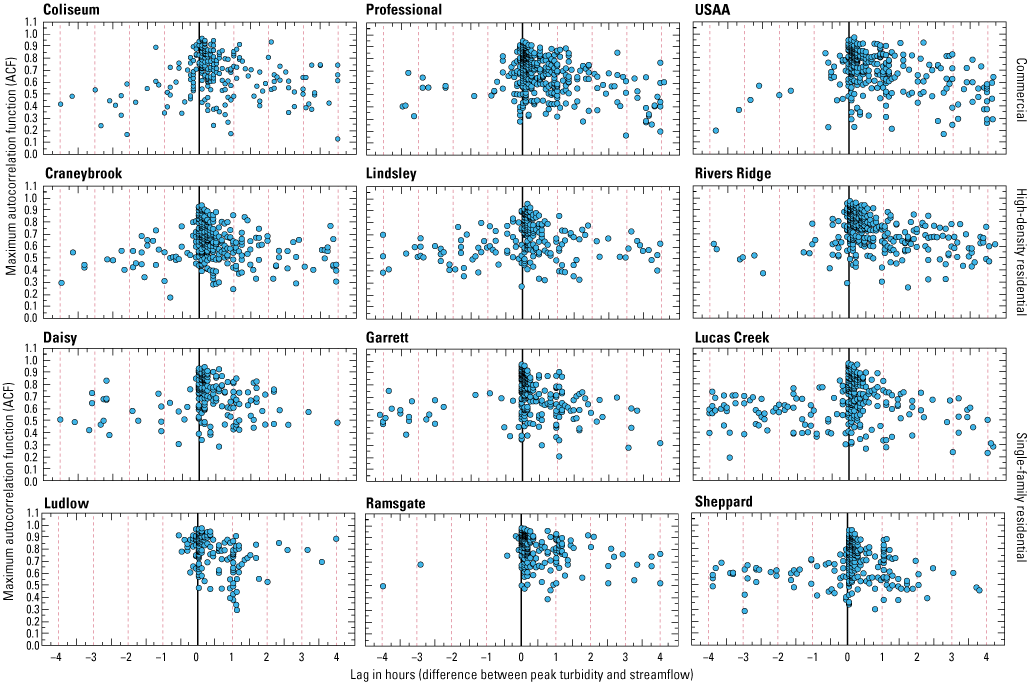
Cross-correlation analysis of total nitrogen (TN) concentration and streamflow. Positive lag values on the x-axis indicate that peak TN preceded peak streamflow, whereas negative values indicate that peak streamflow preceded peak TN. Each lag unit represents a one-hour difference between peak TN and streamflow. The strength of the relation between TN and streamflow is represented by the correlation function on the y-axis (1 equals perfect correlation, 0 equals no correlation). Station names are defined in table 1.
Although M(V) curves confirm that loadings of N were greater in the beginning phase of the runoff response, strict criterion (ΔMax ≥ 0.2) of a first flush was rarely met (table 9; fig. 30). On average, the ΔMax criterion was exceeded only about 20 percent of the time across all 12 stations, mobilizing about 50 percent of the TN load in the initial 39 percent of stormflow volume. Delta-max scores were highest in COM watersheds, but not statistically different from scores for the two residential types of land use. Relatively low occurrences of a first flush for TN suggest that sources are less directly connected to the stormwater system. For example, NO3- and dissolved organic N may be flushed out of soils in residential lands and onto impervious surfaces connected to stormwater infrastructure; however, this process first requires soil saturation. Further, loadings of the various forms of N—dissolved versus particulate and organic versus inorganic—can be staggered in time and therefore reduce the first-flush effect. For example, previous studies have reported a rapid first flush of particulate organic N followed by decreasing concentrations at peak streamflow because of dilution. Concentrations of dissolved N (primarily NO3-) then peak on the receding limb of the storm hydrograph and remain elevated for several subsequent days after the event, responding to higher inputs from interflow (Fletcher and others, 2004; Taylor and others, 2005).
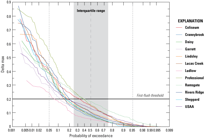
Frequency distribution of delta maximum for total nitrogen. Values greater than 0.2 indicate a first flush based on Geiger (1987).
Table 9.
Summary of mean total nitrogen (TN) mass-volume (M[V]) curves.[Unit values of streamflow and estimations of TN for each extracted storm event are available in the associated data release (Porter, 2022). Station names and land-use types are defined in table 1. All monitoring stations, unless otherwise stated, are at storm drains. N, number of; ΔMax, delta maximum]
The predictive power of TN load and concentration models developed in this study was weaker than that of models for TP or TSS but stronger than the predictive power of similar models for urban stream monitoring stations in Virginia (Porter and others, 2020; Jastram, 2014). The relative strength of these models likely is related to the high proportion of particulate organic nitrogen, which is well predicted by streamflow and turbidity terms. Most models also contained an SC term, a proxy for dissolved solids (such as NO3-), and a seasonal term to account for temporal fluctuations of inputs and speciation. Total nitrogen models accounted for on average 95 percent of the variability in loads and 53 percent in concentrations (app. 1, table 1.13). Total Kjeldahl nitrogen, TON, and NO3- models explained a similar degree of variance in loads and slightly greater variance in concentrations (> 60 percent; app. 1, tables 1.14, 1.15, and 1.16). On average, TN, TKN, TON, and NO3- models were efficient (Nash-Sutcliffe > 0.7) and had low bias (< 3 percent), suggesting accurate predictions of loads. Model coefficients and unit-value estimates of load and yield are published (Porter, 2022).
Yields of TN, TKN, and TON varied across stations and with land-use types, though no effect of land use was observed for NO3- yields (fig. 31; figs. 2.3, 2.4, and 2.5). The average annual yield across all stations for TN, TKN, TON, and NO3- was 10.2 lbs/acre, 7.3 lbs/acre, 6.3 lbs/acre, and 3.0 lbs/acre, respectively (table 10; tables 1.17, 1.18, and 1.19). Over the study period, median annual TN yields were highest at Professional (14.8 lbs/acre) and USAA (14.6 lbs/acre), despite having two of the three lowest median annual concentrations; the lowest median yields occurred at Garrett and Lindsley (5.9 lbs/acre). In COM watersheds, low concentrations are offset by high rates of runoff, producing elevated constituent yields. Total nitrogen yields determined from samples collected in this study were composed primarily of organic N; therefore, the distribution of annual TKN and TON yields across the 12 stations were similar to those of TN. Total nitrogen, TKN, and TON yields were strongly correlated to annual streamflow yield (figs. 2.1D, E, and F), highlighting the importance of particulate wash off in the transport of nitrogen in all its forms. These patterns are consistent with those found in other studies of urban streams in which substantial decreases in N retention were observed between dry and wet years (Duncan and others, 2017; Jastram, 2014; O’Driscoll and others, 2010; Porter and others, 2020). Nitrate was poorly related to annual streamflow yield (app. 2, fig. 2.1G). Annual streamflow yields were predominantly affected by the volume and recurrence of stormflows, whereas 53 percent of the annual NO3- load, on average, was conveyed during base flows.
Table 10.
Summary of annual total nitrogen loads and yields at each monitoring station for water years 2016 through 2020.[Station names and land-use types are defined in table 1. All monitoring stations, unless otherwise stated, are at storm drains. A water year begins October 1 and ends September 30 of the following year. TN, total nitrogen; NA, not applicable]
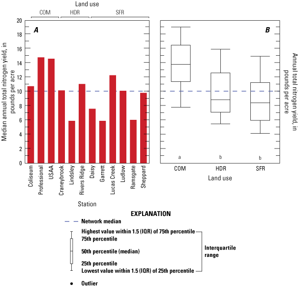
A, Total nitrogen yields for water years 2016 through 2020 at each of the 12 monitoring stations and B, annual yields grouped by land-use type over the same period. A water year begins October 1 and ends September 30. Non-matching letters denote statistical significance based on p less than or equal to 0.05. Station names and land-use acronyms defined in table 1.
The median annual TN yield for the 12 monitoring stations in the Hampton Roads study (10.0 lbs/acre) was similar to that for monitored streams in Fairfax County, Virginia (8.5 lbs/acre), and significantly higher than median values for monitored streams in Gwinnett County, Georgia (5.4 lbs/acre), and the CB-NTN stations (5.4 lbs/acre; fig. 32). Conversely, NO3- yields were significantly lower in Hampton Roads (2.7 lbs/acre) than in the monitored Fairfax County streams (4.4 lbs/acre) and the CB-NTN (3.3 lbs/acre), but similar to those in Gwinnett County (2.5 lbs/acre). Yields of neither TON nor TKN were available from the comparison networks; however, average annual TN and NO3- yields from those networks can be used to infer regional differences in the composition of N loads. As with other constituents, care must be taken when comparing yields across these networks because of dissimilarities in stream order and watershed size. Elevated TON yields in Hampton Roads may also highlight an important difference in carbon processing between buried stormwater conveyances and natural earthen streams. Natural streams typically consist of a series of erosional and depositional zones. Depositional areas commonly serve as “hotspots” for the microbial decomposition of allochthonous materials and transformation of nutrients (Kaushal and Belt, 2012). Traditional engineered stormwater systems are designed to discourage the deposition and retention of materials to prevent the buildup of materials that reduce flow capacity and efficiency. Further, the lack of light and natural habitat is not conducive to microbial communities or benthic macroinvertebrates, which can process allochthonous nutrients and carbon inputs (Santhana Kumar and others, 2017). These factors may result in greater export of organic matter and organic N from lands drained by engineered stormwater conveyances than by natural streams.
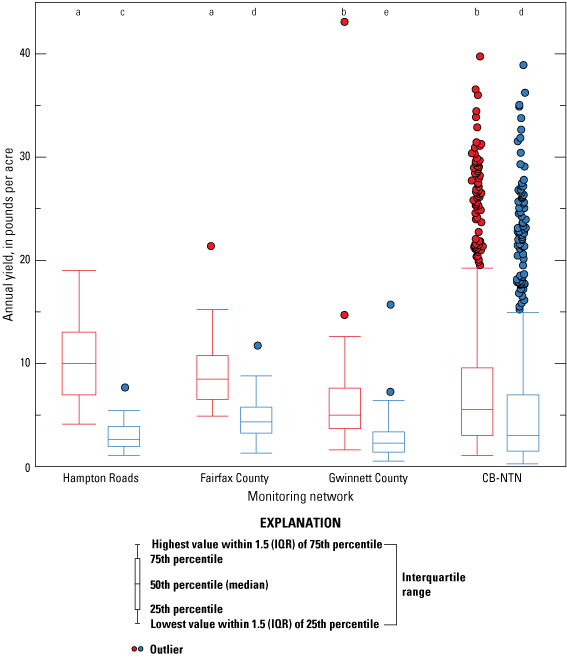
Boxplots of annual total nitrogen (red) and nitrate (blue) yields from four monitoring networks—Hampton Roads and Fairfax County, Virginia, Gwinnett County, Georgia, and the Chesapeake Bay Non-tidal Network (CB-NTN). Non-matching letters denote statistically significant differences based on p less than or equal to 0.05 in total phosphorus and orthophosphate between networks.
Summary
Nonpoint-source pollution is a key driver of aquatic impairment in Chesapeake Bay. In response to decades of declining health, a total maximum daily load was established in 2010 to set annual limits on sediment, phosphorus, and nitrogen loadings to the estuary. Urbanization can substantially alter nonpoint-source loadings to streams, and although a growing body of literature has documented these processes, conditions may vary widely by region or physiographic province (PP). Hampton Roads, a metropolitan region within the Coastal Plain PP of Virginia, has undergone substantial population growth over the last half century. Urbanization has led to an increase in landscape features such as impervious surfaces (roads, sidewalks, parking lots, rooftops), compacted soils, and channelized stormwater conveyance networks, which can alter watershed hydrology and limit or altogether bypass natural processes that facilitate sediment and nutrient attenuation or removal. Decades of monitoring has supported the development of tools used to allocate load reductions across the Chesapeake Bay watershed; however, small urban watersheds, such as those in the Hampton Roads region of the Coastal Plain PP, may not be well represented by current models.
The U.S. Geological Survey (USGS), in partnership with the Hampton Roads Sanitation District (HRSD) and in cooperation with the Hampton Roads Planning District Commission (HRPDC), established a long-term stormwater monitoring program to characterize water quality and streamflow conditions and compute average-annual sediment and nutrient loading rates across the three dominant land-use types in the region—commercial (COM), high-density residential (HDR), and single-family residential (SFR). Monitoring began at 8 stations in 2015, and at an additional 4 stations in 2016. A complete annual (WY) timeseries was required for many of the analyses presented herein; therefore, data collected in WY 2015 are not included in this report. This report summarizes data collected from WY 2016 through WY 2020 to (1) assess patterns in streamflow and water chemistry; (2) compute annual sediment and nutrient loads; and (3) compare annual-loading rates to other monitoring networks.
Annual precipitation volume was highest in water year (WY) 2016 and was close to the 5-year average WYs 2017 through 2020. In all years, days with rainfall greater than 1 inch were rare, but accounted for much of the annual total volume. Patterns in streamflow are similar to those observed in other urban watersheds. Comparisons of base flow and flashiness indices between study watersheds and reference streamgages throughout the Coastal Plain PP highlight changes in watershed hydrology related to urban activities. Base-flow indices, which indicate the percentage of streamflow contributed by groundwater discharges to streams, were significantly lower at network stations than at the reference streamgages. Likewise, stream flashiness indices, measures of oscillations in the flow hydrograph, were much higher than at the reference streamgages. These differences reflect a decrease in infiltration and subsequent increase in storm runoff as a result of urbanization. Stream flashiness was strongly and positively related to impervious land cover and negatively to watershed area. Flashiness was greatest in the HDR and COM watersheds, followed by that in SFR watersheds, and in the non-urban reference station watersheds. Annual streamflow yields and runoff ratios varied across the three land-use types, increasing along a development gradient with the lowest values associated with SFR watersheds and highest values in the COM watersheds. Most of the study watersheds were stormflow dominated, so event-based analyses were conducted on 200–535 storms at each monitoring station to investigate spatial and seasonal patterns in watershed runoff response. Stormflow yields, runoff ratios, and peak flows were highest in COM watersheds. In contrast, longer duration events, longer time to peak streamflow, and a longer lag between peak precipitation and peak streamflow were documented in SFR watersheds. Variability in flow characteristics between SFR and HDR watersheds was less pronounced than in COM watersheds and were station dependent. Land-cover attributes such as tree canopy over turf and watershed area were well correlated with lower magnitude storms, less runoff per unit rainfall, and a slower hydrologic response. Additionally, event-based metrics varied seasonally because of regional meteorological patterns. Higher intensity and often shorter duration convective storms produced hydrologic responses of greater magnitude and rate of change during warm months than in cool months.
Water temperatures varied seasonally, but diel fluctuations in natural streams were low at most stations because of buffering in subterranean stormwater conveyances. Spatial variability in water temperature was related to watershed imperviousness, with highest temperatures observed in watersheds with greatest impervious cover.
Median specific conductance (SC) values ranged from 191 to 675 microsiemens per centimeter (μS/cm) across the 12 monitoring stations, which are higher than typical conductance levels of less than 100 μS/cm in undeveloped Coastal Plain PP watersheds. Elevated SC may result from anthropogenic inputs, such as the weathering of concrete materials within the stormwater conveyance system itself. The highest median values of conductance also may be related to natural interchange of more saline water from adjacent tidal waters and the surficial aquifer. Specific conductance did not vary across land-use types but was significantly higher in the cool season (October–March) than in the warmer months and thus may be related to the use of road de-icing and anti-icing salts prior to winter storm events.
Concentrations of total suspended solids (TSS) and total phosphorus (TP) were positively correlated to streamflow, whereas total nitrogen (TN) varied little across the monitoring network. Nitrogen composition, however, varied with hydrologic condition, as nitrate plus nitrite (NO3-) dominance during base flows shifted to total organic nitrogen (TON) dominance during periods of runoff. This shift results when higher concentrations of NO3- in discharging groundwater become diluted by lower concentrations of NO3- in runoff; simultaneously, the increase in streamflow facilitates entrainment of organic N-bound particulates. Phosphorus composition varied seasonally–—the proportion of orthophosphate (PO43-) was highest in samples collected from stations draining residential lands and was elevated in summer and fall. Elevated PO43- concentrations in summer and fall months also may be related to microbial degradation of organic matter, temperature-mediated desorption, and leaching from unbagged grass clippings and leaf litter. For all three constituents (sediment and the nutrients N and P), concentrations were highest in SFR watersheds, whereas yields of total suspended solids and total nitrogen were greatest in COM watersheds; total phosphorus yields did not vary across land-use types. This seeming contradiction in concentration and yield across land-use types resulted from spatial differences in streamflow yield.
Network median concentrations of TSS, TP, TN, and nitrogen subspecies at the Hampton Roads monitoring stations were compared to those at stations in similar land-use types (residential and COM) in the National Stormwater Quality Database (NSQD) as well as in a subset of NSQD stations location in the Hampton Roads region. The Hampton Roads network median for each constituent was lower than the national median. The network median TSS and TP concentration was similar to the subset of NSQD stations in Hampton Roads, whereas TN, total Kjeldahl nitrogen (TKN) and NO3- concentrations was lower.
The network average TSS yield in Hampton Roads was significantly lower than in comparison networks in Fairfax County, Virginia, and in Gwinnett County, Georgia; differences that may be reflective of differences in the unique topographic and soil characteristics of the Coastal Plain PP versus those in the Piedmont PP, as well as differences between earthen streams and engineered concrete stormwater conveyances. Loading rates in streams in the Piedmont PP result from large available pools of legacy sediment and high rates of soil erosion, whereas very little fine-grained sediment is transported from the characteristically low-gradient sandy streams of the Coastal Plain PP. Further, TSS yields typically are inversely related to watershed size because of a lack of opportunity for in-channel and floodplain attenuation. Regardless, yields from Hampton Roads were similar to those in substantially larger CB-NTN watersheds, suggesting a lack of available substrate or physical processes capable of entraining and transporting particulate matter.
The average annual TP yield in Hampton Roads was higher than averages reported in comparison studies. Elevated TP yields were driven primarily by higher PO43- yields and may be related to unique soil and geological features of the Coastal Plain PP that limit phosphorus retention. Phosphorus loads commonly have been associated with sediment transport, most notably in Virginia’s upland areas; however, relatively low TSS yields in Hampton Roads suggest non-sediment related sources of P. Total nitrogen yields were similar between the Hampton Roads and Fairfax County networks; however, composition did vary, with greater total organic nitrogen yields in Hampton Roads and greater NO3- yields in Fairfax County. Similar to findings in other urban monitoring studies, TN yields were strongly correlated to annual streamflow volume.
Cross-correlation analyses and mass-volume curves were used to assess the timing of sediment and nutrient loadings. Most of the TSS and TP was typically transported during the initial phase of a storm-runoff event, commonly termed the “first flush.” This suggests TSS and TP were quickly delivered to the storm conveyances from storages within the pipe network and accretion on impervious surfaces, and available source pools were rapidly depleted. Although TN concentrations typically peaked within an hour of peak streamflow, reflecting the particulate dominance of TN during stormflows, and loadings were greater during the early phase of most storm events, the first-flush criterion was rarely met. This suggests that the most abundant sources of TN in these watersheds are not as directly connected to the stormwater-conveyance system as TSS and TP.
References Cited
Allen, D.M., 1974, The relationship between variable selection and data agumentation [sic] and a method for prediction: Technometrics, v. 16, no. 1, p. 125–127, accessed June 2020. https://doi.org/10.1080/00401706.1974.10489157.
Alvarez-Cobelas, M., Sánchez-Carrillo, S., Angeler, D.G., and Sánchez-Andrés, R., 2009, Phosphorus export from catchments—A global view: Journal of the North American Benthological Society, v. 28, no. 4, p. 805–820, accessed May 2021. https://doi.org/10.1899/09-073.1.
Arnold, C.L., Jr., and Gibbons, C.J., 1996, Impervious surface coverage—The emergence of a key environmental indicator: Journal of the American Planning Association, v. 62, no. 2, p. 243–258, accessed August 2020. https://doi.org/10.1080/01944369608975688.
Ator, S.W., and Denver, J.M., 2015, Understanding nutrients in the Chesapeake Bay watershed and implications for management and restoration-the Eastern Shore: U.S. Geological Survey Circular 1406 v. 1.2, 72 p., accessed June 2021 at https://doi.org/10.3133/cir1406.
Ator, S.W., Brakebill, J.W., and Blomquist, J.D., 2011, Sources, fate, and transport of nitrogen and phosphorus in the Chesapeake Bay watershed—An empirical model: U.S. Geological Survey Scientific Investigations Report 2011–5167, 27 p., accessed April 2020 at https://doi.org/10.3133/sir20115167.
Aulenbach, B.T., Kolb, K., Joiner, J.K., and Knaak, A.E., 2022, Hydrology and water quality in 15 watersheds in DeKalb County, Georgia, 2012–16: U.S. Geological Survey Scientific Investigations Report 2021-5126, 105 p., accessed June 2022 at https://doi.org/10.3133/sir20215126.
Aulenbach, B.T., Joiner, J.K., and Painter, J.A., 2017, Hydrology and water quality in 13 watersheds in Gwinnett County, Georgia, 2001–15: U.S. Geological Survey Scientific Investigations Report 2017–5012, 82 p., accessed February 2021 at https://doi.org/10.3133/sir20175012.
Aura, E., 1978, Determination of available soil phosphorus by chemical methods: Agricultural and Food Science, v. 50, no. 4, p. 305–316, accessed June 2020. https://doi.org/10.23986/afsci.71982.
Baker, D.B., Richards, R.P., Loftus, T.T., and Kramer, J.W., 2004, A new flashiness index—Characteristics and applications to midwestern rivers and streams: Journal of the American Water Resources Association, v. 40, no. 2, p. 503–522, accessed June 2020. https://doi.org/10.1111/j.1752-1688.2004.tb01046.x.
Ballard, R., and Fiskell, J.G.A., 1974, Phosphorus retention in Coastal Plain forest soils—I. Relationship to soil properties: Soil Science Society of America Journal, v. 38, no. 2, p. 250–255, accessed August 2020. https://doi.org/10.2136/sssaj1974.03615995003800020015x.
Barber, L.B., Murphy, S.F., Verplanck, P.L., Sandstrom, M.W., Taylor, H.E., and Furlong, E.T., 2006, Chemical loading into surface water along a hydrological, biogeochemical, and land use gradient—A holistic watershed approach: Environmental Science & Technology, v. 40, no. 2, p. 475–486, accessed January 2020. https://doi.org/10.1021/es051270q.
Bell., McMillan, S.K., Clinton, S.M., and Jefferson, A.J., 2016, Hydrologic response to stormwater control measures in urban watersheds: Journal of Hydrology, v. 541, p. 1488–1500, accessed October 2021. https://doi.org/10.1016/j.jhydrol.2016.08.049.
Bertrand-Krajewski, J.-L., Chebbo, G., and Saget, A., 1998, Distribution of pollutant mass vs volume in stormwater discharges and the first flush phenomenon: Water Research, v. 32, no. 8, p. 2341–2356, accessed June 2020. https://doi.org/10.1016/S0043-1354(97)00420-X.
Bettez, N.D., and Groffman, P.M., 2013, Nitrogen deposition in and near an urban ecosystem: Environmental Science & Technology, v. 47, no. 11, p. 6047–6051, accessed April 2021. https://doi.org/10.1021/es400664b.
Blume, T., Zehe, E., and Bronstert, A., 2007, Rainfall—Runoff response, event-based runoff coefficients and hydrograph separation: Hydrological Sciences Journal, v. 52, no. 5, p. 843–862, accessed June 2020. https://doi.org/10.1623/hysj.52.5.843.
Bonneau, J., Fletcher, T.D., Costelloe, J.F., and Burns, M.J., 2017, Stormwater infiltration and the ‘urban karst’—A review: Journal of Hydrology, v. 552, p. 141–150, accessed March 2021. https://doi.org/10.1016/j.jhydrol.2017.06.043.
Brakebill, J.W., Ator, S.W., and Schwarz, G.E., 2010, Sources of suspended-sediment flux in streams of the Chesapeake Bay Watershed—A regional application of the SPARROW model: Journal of the American Water Resources Association, v. 46, no. 4, p. 757–776, accessed June 2021. https://doi.org/10.1111/j.1752-1688.2010.00450.x.
Bratt, A.R., Finlay, J.C., Hobbie, S.E., Janke, B.D., Worm, A.C., and Kemmitt, K.L., 2017, Contribution of leaf litter to nutrient export during winter months in an urban residential Watershed: Environmental Science & Technology, v. 51, no. 6, p. 3138–3147, accessed January 2021. https://doi.org/10.1021/acs.est.6b06299.
Brown, V.A., McDonnell, J.J., Burns, D.A., and Kendall, C., 1999, The role of event water, a rapid shallow flow component, and catchment size in summer stormflow: Journal of Hydrology, v. 217, no. 3–4, p. 171–190, accessed February 2022. https://doi.org/10.1016/S0022-1694(98)00247-9.
Bruland, G.L., and DeMent, G., 2009, Phosphorus sorption dynamics of Hawaii’s coastal wetlands: Estuaries and Coasts, v. 32, no. 5, p. 844–854, accessed January 2021. https://doi.org/10.1007/s12237-009-9201-9.
Bussi, J., Musso, M., Quevedo, A., Faccio, R., and Romero, M., 2017, Structural and catalytic stability assessment of Ni-La-Sn ternary mixed oxides for hydrogen production by steam reforming of ethanol: Catalysis Today, v. 296, p. 154–162, accessed December 2021. https://doi.org/10.1016/j.cattod.2017.04.024.
Carey, R.O., Hochmuth, G.J., Martinez, C.J., Boyer, T.H., Dukes, M.D., Toor, G.S., and Cisar, J.L., 2013, Evaluating nutrient impacts in urban watersheds—Challenges and research opportunities: Environmental Pollution, v. 173, p. 138–149, accessed March 2021. https://doi.org/10.1016/j.envpol.2012.10.004.
Carpenter, S.R., Caraco, N.F., Correll, D.L., Howarth, R.W., Sharpley, A.N., and Smith, V.H., 1998, Nonpoint pollution of surface waters with phosphorus and nitrogen: Ecological Applications, v. 8, no. 3, p. 559–568, accessed June 2021. https://doi.org/10.1890/1051-0761(1998)008[0559:NPOSWW]2.0.CO;2.
Casey, R.E., Lev, S.M., and Snodgrass, J.W., 2012, Stormwater ponds as a source of long-term surface and ground water salinisation: Urban Water Journal, v. 10, no. 3, p. 145–153, accessed May 2022. https://doi.org/10.1080/1573062X.2012.716070.
Chesapeake Bay Program Office, 2018, High-resolution land cover data for Chesapeake Bay watershed counties: Chesapeake Conservancy web page, accessed June 2018 at https://chesapeakeconservancy.org/conservation-innovation-center-2/high-resolution-data/land-use-data-project/.
Chesapeake Bay Program, 2020, Chesapeake Assessment and Scenario Tool (CAST) Version 2019. Chesapeake Bay Program Office, accessed June 2022 at https://cast.chesapeakebay.net/.
Cohn, T.A., Gilroy, E.J., and Baier, W.G., 1992, Estimating fluvial transport of trace constituents using a regression model with data subject to censoring: American Statistical Association Section on Statistics and the Environment, proceedings, 9 p., accessed January 2018 at https://www.timcohn.com/Publications/CohnGilroyBaier1992.pdf.
Conley, D.J., Paerl, H.W., Howarth, R.W., Boesch, D.F., Seitzinger, S.P., Havens, K.E., Lancelot, C., and Likens, G.E., 2009, Controlling eutrophication—Nitrogen and phosphorus: Science, v. 323, no. 5917, p. 1014–1015, accessed October 2019. https://doi.org/10.1126/science.1167755.
Correll, D.L., 1998, The role of phosphorus in the eutrophication of receiving waters—A review: Journal of Environmental Quality, v. 27, no. 2, p. 261–266, accessed August 2019. https://doi.org/10.2134/jeq1998.00472425002700020004x.
Corsi, S.R., Graczyk, D.J., Geis, S.W., Booth, N.L., and Richards, K.D., 2010, A fresh look at road salt—Aquatic toxicity and water-quality impacts on local, regional, and national scales: Environmental Science & Technology, v. 44, no. 19, p. 7376–7382, accessed January 2021. https://doi.org/10.1021/es101333u.
Coulter, C.B., Kolka, R.K., and Thompson, J.A., 2004, Water quality in agricultural, urban, and mixed land use watersheds: Journal of the American Water Resources Association, v. 40, no. 6, p. 1593–1601, accessed December 2021. https://doi.org/10.1111/j.1752-1688.2004.tb01608.x.
Cox, F.R., and Hendricks, S.E., 2000, Soil test phosphorus and clay content effects on runoff water quality: Journal of Environmental Quality, v. 29, no. 5, p. 1582–1586, accessed March 2017. https://doi.org/10.2134/jeq2000.00472425002900050027x.
Critchlow, D.E., and Flinger, M.A., 1991, On distribution-free multiple comparisons in the one-way analysis of variance: Communications in Statistics - Theory and Methods, v. 20, no. 1, p. 127-139, accessed January 2021 at https://doi.org/10.1080/03610929108830487.
Davidson, E.A., Savage, K.E., Bettez, N.D., Marino, R., and Howarth, R.W., 2010, Nitrogen in runoff from residential roads in a coastal area: Water, Air, and Soil Pollution, v. 210, no. 1–4, p. 3–13, accessed January 2020. https://doi.org/10.1007/s11270-009-0218-2.
Davies, P.J., Wright, I.A., Jonasson, O.J., and Findlay, S.J., 2010a, Impact of concrete and PVC pipes on urban water chemistry: Urban Water Journal, v. 7, no. 4, p. 233–241, accessed April 2020. https://doi.org/10.1080/1573062X.2010.484502.
Davies, P., Wright, I., Jonasson, J., and Findlay, S., 2010b, Impact on runoff quality by the concrete drainage system, in National Conference of the Stormwater Industry Association of Australia (1st: 2010)—Proceedings of Stormwater 2010, 1st National Conference of the Stormwater Industry Association of Australia, 8-12 November 2010, Sydney, Australia: Stormwater Industry Association of Australia, p. 1–12.
Davies, P.J., Wright, I.A., Jonasson, O.J., and Findlay, S.J., 2010c, The effect of the in-transport process on urban water chemistry—an examination of the contribution of concrete pipes and gutters on urban water quality, in Mouritz, M. and Ruprecht, J. eds., NOVATECH 2010—Proceedings of the 7th International Conference on Sustainable Techniques and Strategies in Urban Water Management: Session 2.7, Lyon, France, p. 1–10.
Deletic, A., 1998, The first flush load of urban surface runoff: Water Research, v. 32, no. 8, p. 2462–2470, accessed November 2021. https://doi.org/10.1016/S0043-1354(97)00470-3.
Demars, B.O.L., Manson, J.R., Ólafsson, J.S., Gíslason, G.M., Gudmundsdóttir, R., Woodward, G., Reiss, J., Pichler, D.E., Rasmussen, J.J., and Friberg, N., 2011, Temperature and the metabolic balance of streams: Freshwater Biology, v. 56, no. 6, p. 1106–1121, accessed June 2020. https://doi.org/10.1111/j.1365-2427.2010.02554.x.
Denver, J.M., Cravotta, C.A.I., Ator, S.W., and Lindsey, B.D., 2010, Contributions of phosphorus from groundwater to streams in the Piedmont, Blue Ridge, and Valley and Ridge Physiographic Provinces, Eastern United States: U.S. Geological Survey Scientific Investigations Report 2010–5176, 38 p. [Also available at https://doi.org/10.3133/sir20105176.]
Duan, S., and Kaushal, S.S., 2013, Warming increases carbon and nutrient fluxes from sediments in streams across land use: Biogeosciences, v. 10, no. 2, p. 1193–1207, accessed June 2019. https://doi.org/10.5194/bg-10-1193-2013.
Duan, S., Kaushal, S.S., Groffman, P.M., Band, L.E., and Belt, K.T., 2012, Phosphorus export across an urban to rural gradient in the Chesapeake Bay watershed: Journal of Geophysical Research, v. 117, G1. https://doi.org/10.1029/2011JG001782.
Duncan, J.M., Welty, C., Kemper, J.T., Groffman, P.M., and Band, L.E., 2017, Dynamics of nitrate concentration-discharge patterns in an urban watershed: Water Resources Research, v. 53, no. 8, p. 7349–7365, accessed February 2020. https://doi.org/10.1002/2017WR020500.
Ensign, S.H., Noe, G.B., Hupp, C.R., and Skalak, K.J., 2015, Head-of-tide bottleneck of particulate material transport from watersheds to estuaries: Geophysical Research Letters, v. 42, no. 24, p. 10,671–10,679, accessed April 2021. https://doi.org/10.1002/2015GL066830.
Fink, J.R., Inda, A.V., Tiecher, T., and Barrón, V., 2016, Iron oxides and organic matter on soil phosphorus availability: Ciência e Agrotecnologia, v. 40, no. 4, p. 369–379, accessed March 2021. https://doi.org/10.1590/1413-70542016404023016.
Galloway, J.N., Aber, J.D., Erisman, J.W., Seitzinger, S.P., Howarth, R.W., Cowling, E.B., and Cosby, B.J., 2003, The nitrogen cascade: BioScience, v. 53, no. 4, p. 341–356, accessed June 2021 at https://doi.org/10.1641/0006-3568(2003)053[0341:TNC]2.0.CO;2.
Galloway, J.M., Evans, D.A., and Green, W.R., 2005, Comparability of suspended-sediment concentration and total suspended-solids data for two sites on the L’Anguille River, Arkansas, 2001 to 2003: U.S. Geological Survey Scientific Investigations Report 2005–5193. [Also available at https://doi.org/10.3133/sir20055193.]
Garcia-Fresca, B., 2007, Urban-enhanced groundwater recharge—review and case study of Austin, Texas, USA. Urban groundwater—meeting the challenge, Selected papers from the 32nd International Geological Congress (IGC), Florence, Italy, August 2004. Howard KW (ed). Taylor & Francis/Balkema, Netherlands, pp. 3-18.
Gellis, A.C., Hupp, C.R., Pavich, M.J., Landwehr, J.M., Banks, W.S.L., Hubbard, B.E., Langland, M.J., Ritchie, J.C., and Reuter, J.M., 2009, Sources, transport, and storage of sediment at selected sites in the Chesapeake Bay watershed: U.S. Geological Survey Scientific Investigations Report 2008–5186, 95 p. [Also available at https://doi.org/10.3133/sir20085186.]
Gellis, A.C., Noe, G.B., Clune, J.W., Hupp, C.R., Shenck, E.R., and Schwarz, G.E., 2015, Sources of fine-grained sediment in the Linganore Creek Watershed, Frederick and Carroll Counties, Maryland, 2008–10: U.S. Geological Survey Scientific Investigations Report 2014–5147, 56 p., accessed May 2021 at https://doi.org/10.3133/sir20145147.
Ghane, E., Ranaivoson, A.Z., Feyereisen, G.W., Rosen, C.J., and Moncrief, J.F., 2016, Comparison of contaminant transport in agricultural drainage water and urban stormwater runoff (S. A. Loiselle, Ed.): PLOS ONE, v. 11, no. 12, p. e0167834. [Also available at https://doi.org/10.1371/journal.pone.0167834.
Gippel, C.J., 1995, Potential of turbidity monitoring for measuring the transport of suspended solids in streams: Hydrological Processes, v. 9, no. 1, p. 83–97, accessed September 2022. https://doi.org/10.1002/hyp.3360090108.
Gold, A.C., Thompson, S.P., and Piehler, M.F., 2019, The effects of urbanization and retention-based stormwater management on Coastal Plain stream nutrient export: Water Resources Research, v. 55, no. 8, p. 7027–7046, accessed May 2021. https://doi.org/10.1029/2019WR024769.
Gray, J.R., Glysson, G.D., Turcios, L.M., and Schwarz, G.E., 2000, Comparability of suspended-sediment concentration and total suspended solids data: U.S. Geological Survey Water-Resources Investigations Report 00–4191, 20 p. [Also available at https://doi.org/10.3133/wri004191.]
Griffith, M.B., 2014, Natural variation and current reference for specific conductivity and major ions in wadeable streams of the conterminous USA: Freshwater Science, v. 33, no. 1, p. 1–17, accessed February 2020. https://doi.org/10.1086/674704.
Groffman, P.M., Law, N.L., Belt, K.T., Band, L.E., and Fisher, G.T., 2004, Nitrogen fluxes and retention in urban watershed ecosystems: Ecosystems (New York, N.Y.), v. 7, no. 4, p. 393–403, accessed May 2020. https://doi.org/10.1007/s10021-003-0039-x.
Gupta, K., and Saul, A.J., 1996, Specific relationships for the first flush load in combined sewer flows: Water Research, v. 30, no. 5, p. 1244–1252, accessed August 2019. https://doi.org/10.1016/0043-1354(95)00282-0.
Haq, S., Kaushal, S.S., and Duan, S., 2018, Episodic salinization and freshwater salinization syndrome mobilize base cations, carbon, and nutrients to streams across urban regions: Biogeochemistry, v. 141, no. 3, p. 463–486, accessed October 2020. https://doi.org/10.1007/s10533-018-0514-2.
Harris, W.G., Rhue, R.D., Kidder, G., Brown, R.B., and Littell, R., 1996, Phosphorus retention as related to morphology of sandy coastal plain soil materials: Soil Science Society of America Journal, v. 60, no. 5, p. 1513–1521, accessed March 2021. https://doi.org/10.2136/sssaj1996.03615995006000050032x.
Hatt, B.E., Fletcher, T.D., Walsh, C.J., and Taylor, S.L., 2004, The influence of urban density and drainage infrastructure on the concentrations and loads of pollutants in small streams: Environmental Management, v. 34, no. 1, p. 112–124, accessed January 2021. https://doi.org/10.1007/s00267-004-0221-8.
Helsel, D.R., 2005, Insider censoring—Distortion of data with nondetects: Human and Ecological Risk Assessment, v. 11, no. 6, p. 1127–1137, accessed June 2017. https://doi.org/10.1080/10807030500278586.
Helsel, D.R., Hirsch, R.M., Ryberg, K.R., Archfield, S.A., and Gilroy, E.J., 2020, Statistical methods in water resources: U.S. Geological Survey Techniques and Methods, book 4, chap. A3, 458 p. [Also at available at https://doi.org/10.3133/tm4A3.]
Hillebrand, H., Soininen, J., and Snoeijs, P., 2010, Warming leads to higher species turnover in a coastal ecosystem: Global Change Biology, v. 16, no. 4, p. 1181–1193. https://doi.org/10.1111/j.1365-2486.2009.02045.x.
Hinsinger, P., Brauman, A., Devau, N., Gerard, F., Jourdan, C., Laclau, J.P., Le Cadre, E., Jaillard, B., and Plassard, C., 2011, Acquisition of phosphorus and other poorly mobile nutrients by roots. Where do plant nutrition models fail?: Plant and Soil, v. 348, no. 1–2, p. 29–61, accessed August 2021. https://doi.org/10.1007/s11104-011-0903-y.
Hirsch, R.M., Moyer, D.L., and Archfield, S.A., 2010, Weighted regressions on time, discharge, and season (WRTDS), with an application to Chesapeake Bay river inputs: Journal of the American Water Resources Association, v. 46, no. 5, p. 857–880, accessed September 2019. https://doi.org/10.1111/j.1752-1688.2010.00482.x.
Hobbie, S.E., Baker, L.A., Buyarski, C., Nidzgorski, D., and Finlay, J.C., 2014, Decomposition of tree leaf litter on pavement—Implications for urban water quality: Urban Ecosystems, v. 17, no. 2, p. 369–385, accessed February 2017. https://doi.org/10.1007/s11252-013-0329-9.
Hobbie, S.E., Finlay, J.C., Janke, B.D., Nidzgorski, D.A., Millet, D.B., and Baker, L.A., 2017, Contrasting nitrogen and phosphorus budgets in urban watersheds and implications for managing urban water pollution: Proceedings of the National Academy of Sciences of the United States of America, v. 114, no. 16, p. 4177–4182, accessed November 2021. https://doi.org/10.1073/pnas.1618536114.
Hopkins, K.G., Bhaskar, A.S., Woznicki, S.A., and Fanelli, R.M., 2020, Changes in event-based streamflow magnitude and timing after suburban development with infiltration-based stormwater management: Hydrological Processes, v. 34, no. 2, p. 387–403, accessed March 2021. https://doi.org/10.1002/hyp.13593.
House, W.A., and Denison, F.H., 2002, Total phosphorus content of river sediments in relationship to calcium, iron and organic matter concentrations: Science of the Total Environment, v. 282–283, p. 341–351, accessed November 2020. https://doi.org/10.1016/S0048-9697(01)00923-8.
Hyer, K.E., Denver, J.M., Langland, M.J., Webber, J.S., Bohlke, J.K., and Hively, W.D., 2016, Spatial and temporal variation of stream chemistry associated with contrasting geology and land-use patterns in the Chesapeake Bay Watershed—Summary of results from Smith Creek, Virginia; Upper Chester River, Maryland; Conewago Creek, Pennsylvania; and Difficult Run, Virginia, 2010–2013: U.S. Geological Survey Scientific Investigations Report 2016–5093, p. 236., 211 p., accessed September 2017 at https://doi.org/10.3133/sir20165093.
James, W.F., and Barko, J.W., 2004, Diffusive fluxes and equilibrium processes in relation to phosphorus dynamics in the Upper Mississippi River: River Research and Applications, v. 20, no. 4, p. 473–484, accessed March 2016. https://doi.org/10.1002/rra.761.
Jani, J., Yang, Y., Lusk, M.G., and Toor, G.S., 2020, Composition of nitrogen in urban residential stormwater runoff—Concentrations, loads, and source characterization of nitrate and organic nitrogen: PLoS One, v. 15, no. 2, p. e0229715, accessed November 2021. https://doi.org/10.1371/journal.pone.0229715.
Janke, B.D., Finlay, J.C., and Hobbie, S.E., 2017, Trees and streets as drivers of urban stormwater nutrient pollution: Environmental Science & Technology, v. 51, no. 17, p. 9569–9579, accessed September 2020. https://doi.org/10.1021/acs.est.7b02225.
Jastram, J., 2014, Streamflow, water quality, and aquatic macroinvertebrates of selected streams in Fairfax County, Virginia, 2007–12: U.S. Geological Survey Scientific Investigations Report 2014–5073, 68 p., accessed April 2020 at https://doi.org/10.3133/sir20145073.
Jastram, J.D., Moyer, D.L., and Hyer, K.E., 2009, A comparison of turbidity-based and streamflow-based estimates of suspended-sediment concentrations in three Chesapeake Bay tributaries: U.S. Geological Survey Scientific Investigations Report 2009–5165, 37 p., accessed June 2021 at https://doi.org/10.3133/sir20095165.
Jayakaran, A.D., Libes, S.M., Hitchcock, D.R., Bell, N.L., and Fuss, D., 2014, Flow, organic, and inorganic sediment yields from a channelized watershed in the South Carolina Lower Coastal Plain: Journal of the American Water Resources Association, v. 50, no. 4, p. 943–962, accessed March 2021. https://doi.org/10.1111/jawr.12148.
Johnson, S.L., 2004, Factors influencing stream temperatures in small streams—Substrate effects and a shading experiment: Canadian Journal of Fisheries and Aquatic Sciences, v. 61, no. 6, p. 913–923, accessed February 2019. https://doi.org/10.1139/f04-040.
Johnson, G.H., and Hobbs, C.H., 1990, Pliocene and Pleistocene depositional environments on the York-James Peninsula, Virginia—A field guidebook: Virginia Institute of Marine Sciences, William & Mary, accessed April 2020 at https://doi.org/10.25773/89ge-t255.
Jones, A.S., Stevens, D.K., Horsburgh, J.S., and Mesner, N.O., 2010, Surrogate measures for providing high frequency estimates of total suspended solids and total phosphorus concentrations: Journal of the American Water Resources Association, v. 47, no. 2, p. 239–253, accessed March 2019. https://doi.org/10.1111/j.1752-1688.2010.00505.x.
Kaushal, S.S., 2016, Increased salinization decreases safe drinking water: Environmental Science & Technology, v. 50, no. 6, p. 2765–2766, accessed October 2019. https://doi.org/10.1021/acs.est.6b00679.
Kaushal, S.S., and Belt, K.T., 2012, The urban watershed continuum—Evolving spatial and temporal dimensions: Urban Ecosystems, v. 15, no. 2, p. 409–435, accessed September 2020. https://doi.org/10.1007/s11252-012-0226-7.
Kaushal, S.S., Duan, S., Doody, T., Haq, S., Smith, R.M., Newcomer Johnson, T.A., Stack, W.P., Newcomb, K.D., Gorman, J., Bowman, N., Mayer, P.M., Wood, K.L., and Belt, K.T., 2017, Human-accelerated weathering increases salinization, major ions, and alkalinization in fresh water across land use: Applied Geochemistry, v. 83, p. 121–135, accessed February 2021. https://doi.org/10.1016/j.apgeochem.2017.02.006.
Kaushal, S.S., Groffman, P.M., Likens, G.E., Belt, K.T., Stack, W.P., Kelly, V.R., Band, L.E., and Fisher, G.T., 2005, Increased salinization of fresh water in the northeastern United States: Proceedings of the National Academy of Sciences of the United States of America, v. 102, no. 38, p. 13517–13520, accessed June 2021. https://doi.org/10.1073/pnas.0506414102.
Kaushal, S.S., Likens, G.E., Pace, M.L., Reimer, J.E., Maas, C.M., Galella, J.G., Utz, R.M., Duan, S., Kryger, J.R., Yaculak, A.M., Boger, W.L., Bailey, N.W., Haq, S., Wood, K.L., Wessel, B.M., Park, C.E., Collison, D.C., Aisin, B.Y.I., Gedeon, T.M., Chaudhary, S.K., Widmer, J., Blackwood, C.R., Bolster, C.M., Devilbiss, M.L., Garrison, D.L., Halevi, S., Kese, G.Q., Quach, E.K., Rogelio, C.M.P., Tan, M.L., Wald, H.J.S., and Woglo, S.A., 2021, Freshwater salinization syndrome—From emerging global problem to managing risks: Biogeochemistry, v. 154, no. 2, p. 255–292, accessed March 2021. https://doi.org/10.1007/s10533-021-00784-w.
Kaushal, S.S., Likens, G.E., Pace, M.L., Utz, R.M., Haq, S., Gorman, J., and Grese, M., 2018, Freshwater salinization syndrome on a continental scale: Proceedings of the National Academy of Sciences of the United States of America, v. 115, no. 4, p. E574–E583, accessed April 2020. https://doi.org/10.1073/pnas.1711234115.
Kruskal, W.H., and Wallis, W.A., 1952, Use of ranks in one-criterion variance analysis: Journal of the American Statistical Association, v. 47, no. 260, p. 583–621, accessed June 2021. https://doi.org/10.1080/01621459.1952.10483441.
Kumar, S.V., Pandey, P.K., Anand, T., Bhuvaneswari, R., and Kumar, S., 2017, Effect of periphyton (aquamat) on water quality, nitrogen budget, microbial ecology, and growth parameters of Litopenaeus vannamei in a semi intensive culture system: Aquaculture (Amsterdam, Netherlands), v. 479, p. 240–249, accessed May 2021. https://doi.org/10.1016/j.aquaculture.2017.05.048.
Landers, M.N., and Sturm, T.W., 2013, Hysteresis in suspended sediment to turbidity relations due to changing particle size distributions: Water Resources Research, v. 49, no. 9, p. 5487–5500, accessed October 2018. https://doi.org/10.1002/wrcr.20394.
Langland, M., and Cronin, T., 2003, A summary report of sediment processes in Chesapeake Bay and watershed: U.S. Geological Survey Water-Resources Investigations Report 2003–4123. [Also available at https://pubs.er.usgs.gov/publication/wri034123.]
Latchat Instruments, 2021, Methods List for Automated Ion Analyzers: Flow Injection Analysis—Ion Chromatography—LL022 Revision 17; Hach Company, Loveland Colorado USA, accessed November 2021 at https://www.hach.com/.
LaValle, P.D., 1975, Domestic sources of stream phosphates in urban streams: Water Research, v. 9, no. 10, p. 913–915, accessed January 2020. https://doi.org/10.1016/0043-1354(75)90041-X.
LeBlanc, R.T., Brown, R.D., and FitzGibbon, J.E., 1997, Modeling the effects of land use change on the water temperature in unregulated urban streams: Journal of Environmental Management, v. 49, no. 4, p. 445–469, accessed December 2021. https://doi.org/10.1006/jema.1996.0106.
Lee, J.H., Bang, K.W., Ketchum, L.H., Jr., Choe, J.S., and Yu, M.J., 2002, First flush analysis of urban storm runoff: Science of the Total Environment, v. 293, no. 1, p. 163–175, accessed March 2021. https://doi.org/10.1016/S0048-9697(02)00006-2.
Lee, C.J., and Ziegler, A.C., 2010, Effects of urbanization, construction activity, management practices, and impoundments on suspended-sediment transport in Johnson County, northeast Kansas, February 2006 through November 2008: U.S. Geological Survey Scientific Investigations Report 2010-5128, accessed January 2021 at https://pubs.usgs.gov/sir/2010/5128/.
Lehtoranta, J., and Pitkänen, H., 2003, Binding of phosphate in sediment accumulation areas of the eastern Gulf of Finland, Baltic Sea: Hydrobiologia, v. 492, no. 1–3, p. 55–67, accessed June 2019. https://doi.org/10.1023/A:1024869929510.
Leopold, L.B., 1968, Hydrology for urban land planning—A guidebook on the hydrologic effects of urban land use: U.S. Geological Survey Circular 554, 18 p., accessed August 2018 at https://doi.org/10.3133/cir554.
Leopold, L.B., 1991, Lag times for small drainage basins: Catena, v. 18, no. 2, p. 157–171, accessed March 2020. https://doi.org/10.1016/0341-8162(91)90014-O.
Levesque, V.A., and Oberg, K.A., 2012, Computing discharge using the index velocity method: U.S. Geological Survey Techniques and Methods 3–A23, 148 p., accessed March 2021 at https://doi.org/10.3133/tm3A23.
Li, L., Yin, C., He, Q., and Kong, L., 2007, First flush of storm runoff pollution from an urban catchment in China: Journal of Environmental Sciences (China), v. 19, no. 3, p. 295–299, accessed May 2021. https://doi.org/10.1016/S1001-0742(07)60048-5.
Liu, F., He, J.Z., Colombo, C., and Violante, A., 1999, Competitive adsorption of sulfate and oxalate on goethite in the absence or presence of phosphate: Soil Science, v. 164, no. 3, p. 180–189, accessed February 2016. https://doi.org/10.1097/00010694-199903000-00004.
Lorenz, D., Runkel, R., and De Cicco, L., 2015, rloadest—River load estimation (ver. 0.4.5): U.S. Geological Survey GitHub web page, accessed August 2020 at https://github.com/USGS-R/rloadest.
Luedtke, R.J., and Brusven, M.A., 1976, Effects of sand sedimentation on colonization of stream insects: Journal of the Fisheries Research Board of Canada, v. 33, no. 9, p. 1881–1886, accessed May 2021. https://doi.org/10.1139/f76-240.
Lusk, M.G., and Toor, G.S., 2016, Dissolved organic nitrogen in urban streams—Biodegradability and molecular composition studies: Water Research, v. 96, p. 225–235, accessed March 2021. https://doi.org/10.1016/j.watres.2016.03.060.
Ma, J.S., Khan, S., Li, Y.X., Kim, L.H., Ha, S., Lau, S.L., Kayhanian, M., and Stenstrom, M.K., 2002, First flush phenomena for highways: How it can be meaningfully defined: Proceedings of the Ninth International Conference on Urban Drainage, v. 9, p. 1–11, accessed February 2017 at https://doi.org/10.1061/40644(2002)223.
McFarland, E.R., and Bruce, T.S., 2006, The Virginia Coastal Plain hydrogeologic framework: U.S. Geological Survey Professional Paper 1731, 118 p., 25 pls., accessed March 2020 at https://doi.org/10.3133/pp1731.
McFarland, E.R., 2010, Groundwater-quality data and regional trends in the Virginia Coastal Plain, 1906–2007: U.S, Geological Survey Professional Paper 1772, 86 p., 14 pls., accessed June 2021 at https://doi.org/10.3133/pp1772.
Meng, Z., Yang, Y., Qin, Z., and Huang, L., 2018, Evaluating temporal and spatial variation in nitrogen sources along the lower reach of Fenhe River (Shanxi Province, China): Water (Basel), v. 10, no. 2, p. 231. https://doi.org/10.3390/w10020231.
Merill, L., and Tonjes, D.J., 2014, A review of the hyporheic zone, stream restoration, and means to enhance denitrification: Critical Reviews in Environmental Science and Technology, v. 44, no. 21, p. 2337–2379, accessed July 2021. https://doi.org/10.1080/10643389.2013.829769.
Meybeck, M., 1998, Man and river interface—Multiple impacts on water and particulates chemistry illustrated in the Seine river basin, in Amiard, J.C., Le Rouzic, B., Berthet, B., and Bertru, G., eds., Oceans, Rivers and Lakes—Energy and Substance Transfers at Interfaces: Dordrecht, Springer Netherlands, p. 1–20, accessed May 2021 at https://doi.org/10.1007/978-94-011-5266-2_1.
Moore, J., Fanelli, R.M., and Sekellick, A.J., 2020, High-frequency data reveal deicing salts drive elevated specific conductance and chloride along with pervasive and frequent exceedances of the U.S. Environmental Protection Agency aquatic life criteria for chloride in urban streams: Environmental Science & Technology, v. 54, no. 2, p. 778–789, accessed July 2021. https://doi.org/10.1021/acs.est.9b04316.
Morley, C.L., 1982, A simulation study of the powers of three multiple comparison statistics: The Australian Journal of Statistics, v. 24, no. 2, p. 201–210, accessed February 2020. https://doi.org/10.1111/j.1467-842X.1982.tb00825.x.
Moyer, D.L., and Langland, M.J., 2020, Nitrogen, phosphorus, and suspended-sediment loads and trends measured at the Chesapeake Bay Nontidal Network stations—Water years 1985–2018 (ver. 2.0, May 2020): U.S. Geological Survey data release, accessed May 2021 at https://doi.org/10.5066/P931M7FT.
Mulholland, P.J., Fellows, C.S., Tank, J.L., Grimm, N.B., Webster, J.R., Hamilton, S.K., Martí, E., Ashkenas, L., Bowden, W.B., Dodds, W.K., Mcdowell, W.H., Paul, M.J., and Peterson, B.J., 2001, Inter-biome comparison of factors controlling stream metabolism: Freshwater Biology, v. 46, no. 11, p. 1503–1517, accessed July 2021. https://doi.org/10.1046/j.1365-2427.2001.00773.x.
Nakano, T., Tayasu, I., Yamada, Y., Hosono, T., Igeta, A., Hyodo, F., Ando, A., Saitoh, Y., Tanaka, T., Wada, E., and Yachi, S., 2008, Effect of agriculture on water quality of Lake Biwa tributaries, Japan: Science of the Total Environment, v. 389, no. 1, p. 132–148, accessed September 2020. https://doi.org/10.1016/j.scitotenv.2007.08.042.
Nash, J.E., and Sutcliffe, J.V., 1970, River flow forecasting through conceptual models part I—A discussion of principles: Journal of Hydrology, v. 10, no. 3, p. 282–290, accessed March 2021. https://doi.org/10.1016/0022-1694(70)90255-6.
National Oceanic and Atmospheric Administration, 2022a, NOAA Atlas 14 point precipitation frequency estimates, accessed February 7, 2022, at Precipitation Frequency Data Server (PFDS) at https://hdsc.nws.noaa.gov/hdsc/pfds/pfds_map_cont.html?bkmrk=va.
National Oceanic and Atmospheric Administration, 2022b, National Centers for Environmental Information: U.S. Climate Normals, accessed June 21, 2022, at https://www.ncei.noaa.gov/products/land-based-station/us-climate-normals.
Noe, G.B., and Hupp, C.R., 2009, Retention of riverine sediment and nutrient loads by Coastal Plain floodplains: Ecosystems (New York, N.Y.), v. 12, no. 5, p. 728–746, accessed January 2022. https://doi.org/10.1007/s10021-009-9253-5.
O’Driscoll, M., Clinton, S., Jefferson, A., Manda, A., and McMillan, S., 2010, Urbanization effects on watershed hydrology and in-stream processes in the southern United States: Water (Basel), v. 2, no. 3, p. 605–648, accessed July 2020. https://doi.org/10.3390/w2030605.
Olsen, S.R., and Watanabe, F.S., 1957, A method to determine a phosphorus adsorption maximum of soils as measured by the Langmuir Isotherm: Soil Science Society of America Journal, v. 21, no. 2, p. 144–149, accessed July 2021. https://doi.org/10.2136/sssaj1957.03615995002100020004x.
Paul, M.J., and Meyer, J.L., 2001, Streams in the urban landscape: Annual Review of Ecology and Systematics, v. 32, no. 1, p. 333–365, accessed October 2016. https://doi.org/10.1146/annurev.ecolsys.32.081501.114040.
Peche, A., Graf, T., Fuchs, L., and Neuweiler, I., 2019, Physically based modeling of stormwater pipe leakage in an urban catchment: Journal of Hydrology, v. 573, p. 778–793, accessed August 2021. https://doi.org/10.1016/j.jhydrol.2019.03.016.
Penn, C.J., Mullins, G.L., Zelazny, L.W., and Sharpley, A.N., 2006, Estimating dissolved phosphorus concentrations in runoff from three physiographic regions of Virginia: Soil Science Society of America Journal, v. 70, no. 6, p. 1967–1974, accessed August 2021. https://doi.org/10.2136/sssaj2006.0027.
Petrone, K.C., 2010, Catchment export of carbon, nitrogen, and phosphorus across an agro-urban land use gradient, Swan-Canning River system, southwestern Australia: Journal of Geophysical Research, v. 115, G1, G01016, https://doi.org/. https://doi.org/10.1029/2009JG001051.
Phillips, J.D., and Lutz, J.D., 2008, Profile convexities in bedrock and alluvial streams: Geomorphology, v. 102, no. 3-4, p. 554–566, accessed November 2021. https://doi.org/10.1016/j.geomorph.2008.05.042.
Pitt, R., Maestre, A., and Clary, J., 2018, National Stormwater Quality Database, accessed January 18, 2022, at NSQD Version 4.02 Access Database at https://bmpdatabase.org/national-stormwater-quality-database.
Poff, N.L., Allan, J.D., Bain, M.B., Karr, J.R., Prestegaard, K.L., Richter, B.D., Sparks, R.E., and Stromberg, J.C., 1997, The natural flow regime: Bioscience, v. 47, no. 11, p. 769–784, accessed March 2020. https://doi.org/10.2307/1313099.
Porter, A.J., Webber, J.S., Witt, J.W., and Jastram, J.D., 2020, Spatial and temporal patterns in streamflow, water chemistry, and aquatic macroinvertebrates of selected streams in Fairfax County, Virginia, 2007–18: U.S. Geological Survey Scientific Investigations Report 2020–5061, 106 p., accessed February 2021 at https://doi.org/10.3133/sir20205061.
Porter, A.J., 2022, Inputs and selected outputs used to assess stormwater quality and quantity in twelve urban watersheds in Hampton Roads, Virginia, 2016-2020: U.S. Geological Survey data release. [Also available at https://doi.org/10.5066/P95S9RFV.]
Potter, J.D., McDowell, W.H., Helton, A.M., and Daley, M.L., 2014, Incorporating urban infrastructure into biogeochemical assessment of urban tropical streams in Puerto Rico: Biogeochemistry, v. 121, no. 1, p. 271–286, accessed July 2020. https://doi.org/10.1007/s10533-013-9914-5.
Poulton, B.C., Rasmussen, T.J., and Lee, C.J., 2007, Assessment of biological conditions at selected stream sites in Johnson County, Kansas, and Cass and Jackson Counties, Missouri, 2003 and 2004: U.S. Geological Survey Scientific Investigations Report 2007–5108, 68 p., accessed September 2021 at https://doi.org/10.3133/sir20075108.
Rantz, S.E., 1982, Measurement and computation of streamflow—Volume 1. Measurement of Stage and Discharge: U.S. Geological Survey Water Supply Paper 2175, p. 313. [Also available at https://doi.org/10.3133/wsp2175.]
R Core Team, 2017, R—A language and environment for statistical computing: Vienna, R Foundation for Statistical Computing. [Also available at https://www.R-project.org/.]
Rasmussen, P.P., Gray, J.R., Glysson, G.D., and Ziegler, A.C., 2009a, Guidelines and procedures for computing timeseries suspended-sediment concentrations and loads from in-stream turbidity-sensor and streamflow data: U.S. Geological Survey Techniques and Methods, book 3, chap. C4, 53 p. [Also available at https://doi.org/10.3133/tm3C4.]
Rasmussen, T.J., Poulton, B.C., and Graham, J.L., 2009b, Quality of streams in Johnson County, Kansas, and relations to environmental variables, 2003–07: U.S. Geological Survey Scientific Investigations Report 2009–5235, 84 p., accessed May 2019 at https://pubs.usgs.gov/sir/2009/5235/.
Ratzlaff, J.R., 1994, Mean annual precipitation, runoff, and runoff ratio for Kansas, 1971–1990: Transactions of the Kansas Academy of Science, v. 97, no. 3/4, p. 94. https://doi.org/10.2307/3627776.
Robertson, D.M., Hubbard, L.E., Lorenz, D.L., and Sullivan, D.J., 2018, A surrogate regression approach for computing continuous loads for the tributary nutrient and sediment monitoring program on the Great Lakes: Journal of Great Lakes Research, v. 44, no. 1, p. 26–42, accessed June 2019. https://doi.org/10.1016/j.jglr.2017.10.003.
Robinson, H.K., Hasenmueller, E.A., and Chambers, L.G., 2017, Soil as a reservoir for road salt retention leading to its gradual release to groundwater: Applied Geochemistry, v. 83, p. 72–85, accessed February 2020. https://doi.org/10.1016/j.apgeochem.2017.01.018.
Rose, S., and Peters, N.E., 2001, Effects of urbanization on streamflow in the Atlanta area (Georgia, USA)—A comparative hydrological approach: Hydrological Processes, v. 15, no. 8, p. 1441–1457, accessed March 2020. https://doi.org/10.1002/hyp.218.
Runkel, R.L., Crawford, C.G., and Cohn, T.A., 2004. https://doi.org/10.3133/tm4A5.
Russell, K.L., Vietz, G.J., and Fletcher, T.D., 2017, Global sediment yields from urban and urbanizing watersheds: Earth-Science Reviews, v. 168, p. 73–80, accessed November 2019. https://doi.org/10.1016/j.earscirev.2017.04.001.
Sanford, W., Nelms, D.L., Pope, J.P., and Selnick, D.L., 2012, Quantifying components of the hydrologic cycle in Virginia using chemical hydrograph separation and multiple regression analysis: U.S. Geological Survey Scientific Investigations Report 2011–5198, 152 p., accessed January 2019 at https://doi.org/10.3133/sir20115198.
Sansalone, J.J., and Cristina, C.M., 2004, First flush concepts for suspended and dissolved solids in small impervious watersheds: Journal of Environmental Engineering, v. 130, no. 11, p. 1301–1314, accessed March 2019 at https://doi.org/10.1061/(ASCE)0733-9372(2004)130:11(1301).
Sauer, V.B., and Turnipseed, D.P., 2010, Stage measurement at gaging stations: U.S. Geological Survey Techniques and Methods, book 3, chap. A7, 45 p., accessed January 2015 at https://doi.org/10.3133/tm3A7.
Seitzinger, S.P., and Sanders, R.W., 1997, Contribution of dissolved organic nitrogen from rivers to estuarine eutrophication: Marine Ecology Progress Series, v. 159, p. 1–12, accessed July 2018. https://doi.org/10.3354/meps159001.
Seitzinger, S.P., Sanders, R.W., and Styles, R., 2002, Bioavailability of DON from natural and anthropogenic sources to estuarine plankton: Limnology and Oceanography, v. 47, no. 2, p. 353–366, accessed June 2020. https://doi.org/10.4319/lo.2002.47.2.0353.
Selbig, W.R., 2016, Evaluation of leaf removal as a means to reduce nutrient concentrations and loads in urban stormwater: Science of the Total Environment, v. 571, p. 124–133, accessed August 2021. https://doi.org/10.1016/j.scitotenv.2016.07.003.
Shanley, J.B., 1994, Effects of ion exchange on stream solute fluxes in a basin receiving highway deicing salts: Journal of Environmental Quality, v. 23, no. 5, p. 977–986, accessed June 2021. https://doi.org/10.2134/jeq1994.00472425002300050019x.
Sharp, J.M., Krothe, J.N., Mather, J.D., Garcia-Fresca, B., and Stewart, C.A., 2003, Effects of urbanization on groundwater systems, in Earth Science in the City—A Reader: Washington, D.C., American Geophysical Union. https://doi.org/10.1029/SP056p0257
Sharpley, A.N., 1995, Soil phosphorus dynamics—Agronomic and environmental impacts: Ecological Engineering, v. 5, no. 2–3, p. 261–279, accessed January 2016. https://doi.org/10.1016/0925-8574(95)00027-5.
Sharpley, A.N., Ahuja, L.R., and Menzel, R.G., 1981, The release of soil phosphorus to runoff in relation to the kinetics of desorption: Journal of Environmental Quality, v. 10, no. 3, p. 386–391, accessed June 2019. https://doi.org/10.2134/jeq1981.00472425001000030029x.
Shields, C.A., Band, L.E., Law, N., Groffman, P.M., Kaushal, S.S., Savvas, K., Fisher, G.T., and Belt, K.T., 2008, Streamflow distribution of non-point source nitrogen export from urban-rural catchments in the Chesapeake Bay watershed: Water Resources Research, v. 44, no. 9, accessed December 2020. https://doi.org/10.1029/2007WR006360.
Smith, S.M.C., and Wilcock, P.R., 2015, Upland sediment supply and its relation to watershed sediment delivery in the contemporary mid-Atlantic Piedmont (U.S.A.): Geomorphology, v. 232, p. 33–46, accessed June 2020. https://doi.org/10.1016/j.geomorph.2014.12.036.
Snodgrass, J.W., Moore, J., Lev, S.M., Casey, D.R., Ownby, D.R., Flora, R.F., and Grant, I., 2017, Influence of modern stormwater management practices on transport of road salt to surface waters: Environmental Science & Technology, v. 51, no. 8, p. 4165–4172, accessed January 2019. https://doi.org/10.1021/acs.est.6b03107.
Soldat, D.J., and Petrovic, A.M., 2008, The fate and transport of phosphorus in turfgrass ecosystems: Crop Science, v. 48, no. 6, p. 2051–2065, accessed June 2019. https://doi.org/10.2135/cropsci2008.03.0134.
Sorenson, J.R., 2013, Potential reductions of street solids and phosphorus in urban watersheds from street cleaning, Cambridge, Massachusetts, 2009-11: U.S. Geological Survey Scientific Investigations Report 2012–5292, 66 p., plus appendix 1 on a CD-ROM in pocket, accessed May 2019 at https://doi.org/10.3133/sir20125292.
Soulsby, C., Tetzlaff, D., Rodgers, P., Dunn, S., and Waldron, S., 2006, Runoff processes, stream water residence times and controlling landscape characteristics in a mesoscale catchment—An initial evaluation: Journal of Hydrology, v. 325, no. 1–4, p. 197–221, accessed June 2018. https://doi.org/10.1016/j.jhydrol.2005.10.024.
Spearman, C., 1904, The proof and measurement of association between two things: The American Journal of Psychology, v. 15, no. 1, p. 72–101, accessed June 2021. https://doi.org/10.2307/1412159.
St. Clair, J., Cartier, C., Triantafyllidou, S., Clark, B., and Edwards, M., 2016, Long-term behavior of simulated partial lead service line replacements: Environmental Engineering Science, v. 33, no. 1, p. 53–64, accessed June 2019. https://doi.org/10.1089/ees.2015.0337.
Steele, M.K., and Aitkenhead-Peterson, J.A., 2013, Salt impacts on organic carbon and nitrogen leaching from senesced vegetation: Biogeochemistry, v. 112, no. 1-3, p. 245–259, accessed January 2018. https://doi.org/10.1007/s10533-012-9722-3.
Stenback, G.A., Crumpton, W.G., Schilling, K.E., and Helmers, M.J., 2011, Rating curve estimation of nutrient loads in Iowa rivers: Journal of Hydrology, v. 396, no. 1–2, p. 158–169, accessed July 2019. https://doi.org/10.1016/j.jhydrol.2010.11.006.
Steuer, J., Selbig, W., Hornewer, N.J., and Prey, J., 1997, Sources of contamination in an urban basin in Marquette, Michigan and an analysis of concentrations, loads, and data quality: U.S. Geological Survey Water-Resources Investigations Report 97–4242, 29 p., accessed July 2021 at https://pubs.er.usgs.gov/publication/wri974242.
Tasdighi, A., Arabi, M., and Osmond, D.L., 2017, The relationship between land use and vulnerability to nitrogen and phosphorus pollution in an urban watershed: Journal of Environmental Quality, v. 46, no. 1, p. 113–122, accessed July 2019. https://doi.org/10.2134/jeq2016.06.0239.
Taylor, G.D., Fletcher, T.D., Wong, T.H.F., Breen, P.F., and Duncan, H.P., 2005, Nitrogen composition in urban runoff—Implications for stormwater management: Water Research, v. 39, no. 10, p. 1982–1989, accessed July 2021. https://doi.org/10.1016/j.watres.2005.03.022.
Thomas, P.J., and Harper, J.D., 2009, Soil survey of Tidewater Cities Area, Virginia: United States Department of Agriculture, Virginia Polytechnic Institute and State University, 243 p., accessed September 1, 2001, at https://www.nrcs.usda.gov/Internet/FSE_MANUSCRIPTS/virginia/TidewaterCitiesVA2009/TidewaterCities.pdf.
Thorndahl, S., Balling, J.D., and Larsen, U.B.B., 2016, Analysis and integrated modelling of groundwater infiltration to sewer networks: Hydrological Processes, v. 30, no. 18, p. 3228–3238, accessed February 2021. https://doi.org/10.1002/hyp.10847.
Tufford, D.L., McKellar, H.N., Jr., and Hussey, J.R., 1998, In-stream nonpoint source nutrient prediction with land-use proximity and seasonality: Journal of Environmental Quality, v. 27, no. 1, p. 100–111, accessed January 2019. https://doi.org/10.2134/jeq1998.00472425002700010015x.
Upreti, K., Joshi, S.R., McGrath, J., and Jaisi, D.P., 2015, Factors controlling phosphorus mobilization in a Coastal Plain Tributary to the Chesapeake Bay: Soil Science Society of America Journal, v. 79, no. 3, p. 826–837, accessed March 2018. https://doi.org/10.2136/sssaj2015.03.0117.
U.S. Census Bureau, 2020, Population and housing unit estimates datasets, accessed on June 8, 2022 at https://www.census.gov/programs-surveys/popest/data/data-sets.html.
U.S. Environmental Protection Agency, 2010, Chesapeake Bay total maximum daily load (TMDL) for nitrogen, phosphorus, and sediment: U.S. Environmental Protection Agency, Chesapeake Bay Program Office, Annapolis, Maryland, accessed on July 11, 2021 at https://www.epa.gov/chesapeake-bay-tmdl/chesapeake-bay-tmdl-document.
U.S. Geological Survey, 2006, National field manual for the collection of water-quality data: U.S. Geological Survey Techniques of Water-Resources Investigations, book 9, chap. A4, 166 p. [Also available online at https://doi.org/10.3133/twri09A4.]
U.S. Geological Survey, 2014a, Requirements for the collection, validation, and input of peak-stage verification data at U.S. Geological Survey streamgages: U.S. Geological Survey Technical Memorandum 2014.06; Office of Surface Water, accessed on June 2016 at https://water.usgs.gov/admin/memo/SW/sw14.06_revised.html.
U.S. Geological Survey, 2014b, Updated policy for the evaluation and approval of analytical laboratory performance for Water Mission Area Projects and Programs: U.S. Geological Survey Technical Memorandum 2014.01; Office of Water Quality, accessed on January 2021 at https://water.usgs.gov/admin/memo/QW/qw2014.01.pdf.
U.S. Geological Survey, 2022, USGS water data for the Nation: U.S. Geological Survey National Water Information System database, accessed April 20, 2022, at http://.https://doi.org/10.5066/F7P55KJN.
USDA-NRCS, 1998, Soil map and soil climate map: soil phosphorus retention potential, scale 1:5,000,000, accessed on July 2021 at https://www.nrcs.usda.gov/wps/portal/nrcs/detail/soils/use/worldsoils/?cid=nrcs142p2_054014.
Utz, R.M., Eshleman, K.N., and Hilderbrand, R.H., 2011, Variation in physicochemical responses to urbanization in streams between two Mid-Atlantic physiographic regions: Ecological Applications, v. 21, no. 2, p. 402–415, accessed March 2019. https://doi.org/10.1890/09-1786.1.
Van Breemen, N., Boyer, E.W., Goodale, C.L., Jaworski, N.A., Paustian, K., Seitzinger, S.P., Lajtha, K., Mayer, B., Van Dam, D., Howarth, R.W., Nadelhoffer, K.J., Eve, M., and Billen, G., 2002, Where did all the nitrogen go? Fate of nitrogen inputs to large watersheds in the northeastern U.S.A, in Boyer, E.W., and Howarth, R.W., eds., The Nitrogen Cycle at Regional to Global Scales: Dordrecht, Springer Netherlands, p. 267–293, accessed October 2019 at https://doi.org/10.1007/978-94-017-3405-9_8.
Vaze, J., and Chiew, F.H.S., 2002, Experimental study of pollutant accumulation on an urban road surface: Urban Water, v. 4, no. 4, p. 379–389, accessed November 2018. https://doi.org/10.1016/S1462-0758(02)00027-4.
Wagner, R.J., Boulger, R.W., Oblinger, C.J., and Smith, B.A., 2006, Guidelines and standard procedures for continuous water-quality monitors—Station operation, record computation, and data reporting: U.S. Geological Survey Techniques and Methods 1–D3, 51 p. and 8 attachments; accessed January 2016 at https://doi.org/10.3133/tm1D3.
Wallace, T.A., Ganf, G.G., and Brookes, J.D., 2008, A comparison of phosphorus and DOC leachates from different types of leaf litter in an urban environment: Freshwater Biology, v. 53, no. 9, p. 1902–1913, accessed March 2020. https://doi.org/10.1111/j.1365-2427.2008.02006.x.
Walsh, C.J., Fletcher, T.D., and Ladson, A.R., 2005a, Stream restoration in urban catchments through redesigning stormwater systems—Looking to the catchment to save the stream: Journal of the North American Benthological Society, v. 24, no. 3, p. 690–705, accessed June 2019. https://doi.org/10.1899/04-020.1.
Walsh, C.J., Roy, A.H., Feminella, J.W., Cottingham, P.D., Groffman, P.M., and Morgan, R.P., II, 2005b, The urban stream syndrome—Current knowledge and the search for a cure: Journal of the North American Benthological Society, v. 24, no. 3, p. 706–723, accessed January 2019. https://doi.org/10.1899/04-028.1.
Waschbusch, R., Selbig, W., and Bannerman, R., 1999, Sources of phosphorus in stormwater and street dirt from two urban residential basins in Madison, Wisconsin, 1994-95: U.S. Geological Survey Water-Resources Investigations Report 99–4021, p. 47., accessed March 2020 at https://doi.org/10.3133/wri994021.
Weiss, L.A., 1990, Effects of urbanization on peak streamflows in four Conneticut communities, 1980–84: U.S. Geological Survey Water-Resources Investigation Report 89-4167, p. 45. [Also available at https://doi.org/10.3133/wri894167.]
Wiegner, T.N., Seitzinger, S.P., Glibert, P.M., and Bronk, D.A., 2006, Bioavailability of dissolved organic nitrogen and carbon from nine rivers in the eastern United States: Aquatic Microbial Ecology, v. 43, no. 3, p. 277–287, accessed January 2019. https://doi.org/10.3354/ame043277.
Williams, G.P., 1989, Sediment concentration versus water discharge during single hydrologic events in rivers: Journal of Hydrology, v. 111, no. 1–4, p. 89–106, accessed May 2019. https://doi.org/10.1016/0022-1694(89)90254-0.
Wolf, D., Georgic, W., and Klaiber, H.A., 2017, Reeling in the damages—Harmful algal blooms’ impact on Lake Erie’s recreational fishing industry: Journal of Environmental Management, v. 199, p. 148–157, accessed January 2020. https://doi.org/10.1016/j.jenvman.2017.05.031.
Wood, P.J., 1997, Biological effects of fine sediment in the Lotic Environment: Environmental Management, v. 21, no. 2, p. 203–217, accessed June 2021. https://doi.org/10.1007/s002679900019.
Wood, J.D., Franklin, R.B., Garman, G., McIninch, S., Porter, A.J., and Bukaveckas, P.A., 2014, Exposure to the cyanotoxin microcystin arising from interspecific differences in feeding habits among fish and shellfish in the James River Estuary, Virginia: Environmental Science & Technology, v. 48, no. 9, p. 5194–5202, accessed January 2020. https://doi.org/10.1021/es403491k.
Wright, I.A., Davies, P.J., Findlay, S.J., and Jonasson, O.J., 2011, A new type of water pollution—Concrete drainage infrastructure and geochemical contamination of urban waters: Marine and Freshwater Research, v. 62, no. 12, p. 1355–1361, accessed July 2020. https://doi.org/10.1071/MF10296.
Xu, D., Xu, J., Wu, J., and Muhammad, A., 2006, Studies on phosphorus sorption capacity of substrates used in constructed wetland systems: Chemosphere, v. 63, no. 2, p. 344–352. https://doi.org/10.1016/j.chemosphere.2005.08.036.
Yang, Y., and Toor, G.S., 2018, Stormwater runoff driven phosphorus transport in an urban residential catchment—Implications for protecting water quality in urban watersheds: Scientific Reports, v. 8, no. 11681, 10 p., accessed June 2021 at https://doi.org/10.1038/s41598-018-29857-x.
Zhang, Q., and Blomquist, J.D., 2018, Watershed export of fine sediment, organic carbon, and chlorophyll-a to Chesapeake Bay—Spatial and temporal patterns in 1984–2016: Science of the Total Environment, v. 619–620, p. 1066–1078, accessed December 2020. https://doi.org/10.1016/j.scitotenv.2017.10.279.
Zhang, Q., Brady, D.C., Boynton, W.R., and Ball, W.P., 2015, Long-term trends of nutrients and sediment from the nontidal Chesapeake Watershed—An assessment of progress by river and season: Journal of the American Water Resources Association, v. 51, no. 6, p. 1534–1555, accessed June 2021. https://doi.org/10.1111/1752-1688.12327.
Appendix 1. Reference streamgage stations, principal component loadings, constituent concentrations in water samples, results of hypotheses tests, and load and concentration model diagnostics for stormwater monitoring stations, Hampton Roads, Virginia, 2016-2020
Table 1.1.
Reference streamgages.[mi2, square mile; %, percent; Va, Virginia; Md, Maryland; US, United States; N.C., North Carolina; —, no data – not applicable]
Table 1.2.
Difference in slope, with standard error and p-value for each pairwise comparison from an analysis of covariance testing for differences in the slopes of regression lines for event-based streamflow yield and precipitation volume for all land-use types by type combinations.[Significant differences are based on p less than or equal to 0.05. COM, commercial; HDR, high-density residential; SFR, single-family residential; <, less than]
Table 1.3.
Principal component loadings for event-based streamflow metrics.[PC, principal component; –, negative (number)]
Table 1.4.
Median constituent concentrations in samples collected at each monitoring station and at the network-scale over the study period, presented by the hydrologic condition (base flow or stormflow) in which samples were collected.[Data from U.S. Geological Survey, 2022. COM, commercial; HDR, high-density residential; SFR, single-family residential; TN, total nitrogen; TKN, total Kjeldahl nitrogen; TON, total organic nitrogen; NO3-, nitrate plus nitrite; NH3, ammonia plus ammonium; TP, total phosphorus; PO43-, orthophosphate; TSS, total suspended solids; Coliseum, Storm Drain at Coliseum Drive at Hampton, Virginia (Va.); Professional, Storm Drain at Professional Place near Chesapeake, Va.; USAA, Storm Drain at USAA Drive at Norfolk, Va.; Craneybrook, Storm Drain at Craneybrook Lane at Edgefield, Va.; Lindsley, Storm Drain at Lindsley Drive near Virginia Beach, Va.; Rivers Ridge, Storm Drain at Rivers Ridge Circle near Newport News, Va.; Daisy, Storm Drain at Daisy Drive near Portsmouth, Va.; Garrett, Storm Drain West of Garrett Drive at Hampton, Va.; Lucas Creek, Storm Drain at Lakewood Park Drive near Newport News, Va.; Ludlow, Storm Drain at Ludlow Drive near Kempsville, Va.; Ramsgate, Conveyance Channel at Ramsgate Lane near Great Bridge, Va.; Sheppard, Storm Drain at Sheppard Avenue near Norfolk, Va.]
Table 1.5.
Spearman rank-order correlation coefficients and p-values for relations between water-quality constituents and streamflow at the 12 monitoring stations.[p-value, probability value; COM, commercial; HDR, high-density residential; SFR, single-family residential; TSS, total suspended solids; TP, total phosphorus; TN, total nitrogen; p-value, probability value; Coliseum, Storm Drain at Coliseum Drive at Hampton, Virginia (Va.); Professional, Storm Drain at Professional Place near Chesapeake, Va.; USAA, Storm Drain at USAA Drive at Norfolk, Va.; Craneybrook, Storm Drain at Craneybrook Lane at Edgefield, Va.; Lindsley, Storm Drain at Lindsley Drive near Virginia Beach, Va.; Rivers Ridge, Storm Drain at Rivers Ridge Circle near Newport News, Va.; Daisy, Storm Drain at Daisy Drive near Portsmouth, Va.; Garrett, Storm Drain West of Garrett Drive at Hampton, Va.; Lucas Creek, Storm Drain at Lakewood Park Drive near Newport News, Va.; Ludlow, Storm Drain at Ludlow Drive near Kempsville, Va.; Ramsgate, Conveyance Channel at Ramsgate Lane near Great Bridge, Va.; Sheppard, Storm Drain at Sheppard Avenue near Norfolk, Va.; <, less than; –, negative (number)]
Table 1.6.
Mean concentrations of water-quality constituents in samples from the 12 Hampton Roads monitoring stations, the National Stormwater Quality Database v.4.02, and a subset of those samples collected at various locations throughout the Hampton Roads area.[Data are from U.S. Geological Survey (2022) and Pitt and others (2018). Concentrations are in milligrams per liter. TSS, total suspended solids; TKN, total Kjeldahl nitrogen; NH3, ammonia plus ammonium; NO3-, nitrate plus nitrite; TP, total phosphorus; PO43-, orthophosphate; NSQD, National Stormwater Quality Database v. 4.02; —, no data]
Mean concentrations of water-quality constituents in samples from the National Stormwater Quality Database (NSQD) v.4.02 (Pitt and others, 2018).
Mean concentrations of water-quality constituents in samples from the 12 Hampton Roads monitoring stations (U.S. Geological Survey, 2022; waterdata.usgs.gov/nwis).
Table 1.7.
Load and concentration model R2, bias percentage, Nash-Sutcliffe efficiency index, and model residual variance of total suspended solids load models at the twelve monitoring stations.[COM, commercial; HDR, high-density residential; SFR, single-family residential; Coliseum, Storm Drain at Coliseum Drive at Hampton, Virginia (Va.); Professional, Storm Drain at Professional Place near Chesapeake, Va.; USAA, Storm Drain at USAA Drive at Norfolk, Va.; Craneybrook, Storm Drain at Craneybrook Lane at Edgefield, Va.; Lindsley, Storm Drain at Lindsley Drive near Virginia Beach, Va.; Rivers Ridge, Storm Drain at Rivers Ridge Circle near Newport News, Va.; Daisy, Storm Drain at Daisy Drive near Portsmouth, Va.; Garrett, Storm Drain West of Garrett Drive at Hampton, Va.; Lucas Creek, Storm Drain at Lakewood Park Drive near Newport News, Va.; Ludlow, Storm Drain at Ludlow Drive near Kempsville, Va.; Ramsgate, Conveyance Channel at Ramsgate Lane near Great Bridge, Va.; Sheppard, Storm Drain at Sheppard Avenue near Norfolk, Va.; NA, not applicable; –, negative (number)]
Table 1.8.
Non-parametric Steel-Dwass test on all pairs for hypothesis testing for differences in orthophosphate (PO43-) and particulate plus dissolved organic phosphorus concentration across four seasons. Seasons are defined by the summer and winter solstice and vernal and autumnal equinox.[Season – Season, season minus season for pairwise comparison; p-value, probability value; <, less than]
Table 1.9.
Load and concentration model R2, bias percentage, Nash-Sutcliffe efficiency index, and model residual variance of total phosphorus models at the 12 monitoring stations.[COM, commercial; HDR, high-density residential; SFR, single-family residential; Coliseum, Storm Drain at Coliseum Drive at Hampton, Virginia (Va.); Professional, Storm Drain at Professional Place near Chesapeake, Va.; USAA, Storm Drain at USAA Drive at Norfolk, Va.; Craneybrook, Storm Drain at Craneybrook Lane at Edgefield, Va.; Lindsley, Storm Drain at Lindsley Drive near Virginia Beach, Va.; Rivers Ridge, Storm Drain at Rivers Ridge Circle near Newport News, Va.; Daisy, Storm Drain at Daisy Drive near Portsmouth, Va.; Garrett, Storm Drain West of Garrett Drive at Hampton, Va.; Lucas Creek, Storm Drain at Lakewood Park Drive near Newport News, Va.; Ludlow, Storm Drain at Ludlow Drive near Kempsville, Va.; Ramsgate, Conveyance Channel at Ramsgate Lane near Great Bridge, Va.; Sheppard, Storm Drain at Sheppard Avenue near Norfolk, Va.; NA, not applicable; –, negative (number)]
Table 1.10.
Load and concentration model R2, bias percentage, Nash-Sutcliffe efficiency index, and model residual variance of orthophosphate load models at the 12 monitoring stations.[COM, commercial; HDR, high-density residential; SFR, single-family residential; Coliseum, Storm Drain at Coliseum Drive at Hampton, Virginia (Va.); Professional, Storm Drain at Professional Place near Chesapeake, Va.; USAA, Storm Drain at USAA Drive at Norfolk, Va.; Craneybrook, Storm Drain at Craneybrook Lane at Edgefield, Va.; Lindsley, Storm Drain at Lindsley Drive near Virginia Beach, Va.; Rivers Ridge, Storm Drain at Rivers Ridge Circle near Newport News, Va.; Daisy, Storm Drain at Daisy Drive near Portsmouth, Va.; Garrett, Storm Drain West of Garrett Drive at Hampton, Va.; Lucas Creek, Storm Drain at Lakewood Park Drive near Newport News, Va.; Ludlow, Storm Drain at Ludlow Drive near Kempsville, Va.; Ramsgate, Conveyance Channel at Ramsgate Lane near Great Bridge, Va.; Sheppard, Storm Drain at Sheppard Avenue near Norfolk, Va.; NA, not applicable; –, negative (number)]
Table 1.11.
Summary of annual orthophosphate loads and yields in water years.[A water year begins October 1 and ends September 30 of the following year. COM, commercial; HDR, high-density residential; SFR, single-family residential; Coliseum, Storm Drain at Coliseum Drive at Hampton, Virginia (Va.); Professional, Storm Drain at Professional Place near Chesapeake, Va.; USAA, Storm Drain at USAA Drive at Norfolk, Va.; Craneybrook, Storm Drain at Craneybrook Lane at Edgefield, Va.; Lindsley, Storm Drain at Lindsley Drive near Virginia Beach, Va.; Rivers Ridge, Storm Drain at Rivers Ridge Circle near Newport News, Va.; Daisy, Storm Drain at Daisy Drive near Portsmouth, Va.; Garrett, Storm Drain West of Garrett Drive at Hampton, Va.; Lucas Creek, Storm Drain at Lakewood Park Drive near Newport News, Va.; Ludlow, Storm Drain at Ludlow Drive near Kempsville, Va.; Ramsgate, Conveyance Channel at Ramsgate Lane near Great Bridge, Va.; Sheppard, Storm Drain at Sheppard Avenue near Norfolk, Va.; NA, not applicable]
Table 1.12.
Non-parametric Steel-Dwass test on all pairs for hypothesis testing for differences in total nitrogen, nitrate plus nitrite (NO3-) and total organic nitrogen concentration across four seasons. Seasons are defined by the summer and winter solstice and vernal and autumnal equinox.[Season – Season, season minus season for pairwise comparison; p-value, probability value; <, less than]
Table 1.13.
Load and concentration model R2, bias percentage, Nash-Sutcliffe efficiency index, and model residual variance of total nitrogen load models at the twelve monitoring stations.[COM, commercial; HDR, high-density residential; SFR, single-family residential; Coliseum, Storm Drain at Coliseum Drive at Hampton, Virginia (Va.); Professional, Storm Drain at Professional Place near Chesapeake, Va.; USAA, Storm Drain at USAA Drive at Norfolk, Va.; Craneybrook, Storm Drain at Craneybrook Lane at Edgefield, Va.; Lindsley, Storm Drain at Lindsley Drive near Virginia Beach, Va.; Rivers Ridge, Storm Drain at Rivers Ridge Circle near Newport News, Va.; Daisy, Storm Drain at Daisy Drive near Portsmouth, Va.; Garrett, Storm Drain West of Garrett Drive at Hampton, Va.; Lucas Creek, Storm Drain at Lakewood Park Drive near Newport News, Va.; Ludlow, Storm Drain at Ludlow Drive near Kempsville, Va.; Ramsgate, Conveyance Channel at Ramsgate Lane near Great Bridge, Va.; Sheppard, Storm Drain at Sheppard Avenue near Norfolk, Va.; –, negative (number); NA, not applicable]
Table 1.14.
Load and concentration model R2, bias percentage, Nash-Sutcliffe efficiency index, and model residual variance of total Kjeldahl nitrogen load models at the 12 monitoring stations.[COM, commercial; HDR, high-density residential; SFR, single-family residential; Coliseum, Storm Drain at Coliseum Drive at Hampton, Virginia (Va.); Professional, Storm Drain at Professional Place near Chesapeake, Va.; USAA, Storm Drain at USAA Drive at Norfolk, Va.; Craneybrook, Storm Drain at Craneybrook Lane at Edgefield, Va.; Lindsley, Storm Drain at Lindsley Drive near Virginia Beach, Va.; Rivers Ridge, Storm Drain at Rivers Ridge Circle near Newport News, Va.; Daisy, Storm Drain at Daisy Drive near Portsmouth, Va.; Garrett, Storm Drain West of Garrett Drive at Hampton, Va.; Lucas Creek, Storm Drain at Lakewood Park Drive near Newport News, Va.; Ludlow, Storm Drain at Ludlow Drive near Kempsville, Va.; Ramsgate, Conveyance Channel at Ramsgate Lane near Great Bridge, Va.; Sheppard, Storm Drain at Sheppard Avenue near Norfolk, Va.; –, negative (number); NA, not applicable]
Table 1.15.
Load and concentration model R2, bias percentage, Nash-Sutcliffe efficiency index, and model residual variance of total organic nitrogen load models at the 12 monitoring stations.[COM, commercial; HDR, high-density residential; SFR, single-family residential; Coliseum, Storm Drain at Coliseum Drive at Hampton, Virginia (Va.); Professional, Storm Drain at Professional Place near Chesapeake, Va.; USAA, Storm Drain at USAA Drive at Norfolk, Va.; Craneybrook, Storm Drain at Craneybrook Lane at Edgefield, Va.; Lindsley, Storm Drain at Lindsley Drive near Virginia Beach, Va.; Rivers Ridge, Storm Drain at Rivers Ridge Circle near Newport News, Va.; Daisy, Storm Drain at Daisy Drive near Portsmouth, Va.; Garrett, Storm Drain West of Garrett Drive at Hampton, Va.; Lucas Creek, Storm Drain at Lakewood Park Drive near Newport News, Va.; Ludlow, Storm Drain at Ludlow Drive near Kempsville, Va.; Ramsgate, Conveyance Channel at Ramsgate Lane near Great Bridge, Va.; Sheppard, Storm Drain at Sheppard Avenue near Norfolk, Va.; –, negative (number); NA, not applicable]
Table 1.16.
Load and concentration model R2, bias percentage, Nash-Sutcliffe efficiency index, and model residual variance of nitrate plus nitrite load models at the twelve monitoring stations.[COM, commercial; HDR, high-density residential; SFR, single-family residential; Coliseum, Storm Drain at Coliseum Drive at Hampton, Virginia (Va.); Professional, Storm Drain at Professional Place near Chesapeake, Va.; USAA, Storm Drain at USAA Drive at Norfolk, Va.; Craneybrook, Storm Drain at Craneybrook Lane at Edgefield, Va.; Lindsley, Storm Drain at Lindsley Drive near Virginia Beach, Va.; Rivers Ridge, Storm Drain at Rivers Ridge Circle near Newport News, Va.; Daisy, Storm Drain at Daisy Drive near Portsmouth, Va.; Garrett, Storm Drain West of Garrett Drive at Hampton, Va.; Lucas Creek, Storm Drain at Lakewood Park Drive near Newport News, Va.; Ludlow, Storm Drain at Ludlow Drive near Kempsville, Va.; Ramsgate, Conveyance Channel at Ramsgate Lane near Great Bridge, Va.; Sheppard, Storm Drain at Sheppard Avenue near Norfolk, Va.; –, negative (number); NA, not applicable]
Table 1.17.
Summary of annual total Kjeldahl nitrogen loads and yields.[Years represent water years, which begin October 1 and end September 30 the following year. COM, commercial; HDR, high-density residential; SFR, single-family residential; Coliseum, Storm Drain at Coliseum Drive at Hampton, Virginia (Va.); Professional, Storm Drain at Professional Place near Chesapeake, Va.; USAA, Storm Drain at USAA Drive at Norfolk, Va.; Craneybrook, Storm Drain at Craneybrook Lane at Edgefield, Va.; Lindsley, Storm Drain at Lindsley Drive near Virginia Beach, Va.; Rivers Ridge, Storm Drain at Rivers Ridge Circle near Newport News, Va.; Daisy, Storm Drain at Daisy Drive near Portsmouth, Va.; Garrett, Storm Drain West of Garrett Drive at Hampton, Va.; Lucas Creek, Storm Drain at Lakewood Park Drive near Newport News, Va.; Ludlow, Storm Drain at Ludlow Drive near Kempsville, Va.; Ramsgate, Conveyance Channel at Ramsgate Lane near Great Bridge, Va.; Sheppard, Storm Drain at Sheppard Avenue near Norfolk, Va.; NA, not applicable]
Table 1.18.
Summary of annual total organic nitrogen loads and yields.[Years represent water years, which begin October 1 and end September 30 the following year. COM, commercial; HDR, high-density residential; SFR, single-family residential; Coliseum, Storm Drain at Coliseum Drive at Hampton, Virginia (Va.); Professional, Storm Drain at Professional Place near Chesapeake, Va.; USAA, Storm Drain at USAA Drive at Norfolk, Va.; Craneybrook, Storm Drain at Craneybrook Lane at Edgefield, Va.; Lindsley, Storm Drain at Lindsley Drive near Virginia Beach, Va.; Rivers Ridge, Storm Drain at Rivers Ridge Circle near Newport News, Va.; Daisy, Storm Drain at Daisy Drive near Portsmouth, Va.; Garrett, Storm Drain West of Garrett Drive at Hampton, Va.; Lucas Creek, Storm Drain at Lakewood Park Drive near Newport News, Va.; Ludlow, Storm Drain at Ludlow Drive near Kempsville, Va.; Ramsgate, Conveyance Channel at Ramsgate Lane near Great Bridge, Va.; Sheppard, Storm Drain at Sheppard Avenue near Norfolk, Va.; NA, not applicable]
Table 1.19.
Summary of annual nitrate plus nitrite loads and yields.[Years represent water years, which begin October 1 and end September 30 the following year. COM, commercial; HDR, high-density residential; SFR, single-family residential; Coliseum, Storm Drain at Coliseum Drive at Hampton, Virginia (Va.); Professional, Storm Drain at Professional Place near Chesapeake, Va.; USAA, Storm Drain at USAA Drive at Norfolk, Va.; Craneybrook, Storm Drain at Craneybrook Lane at Edgefield, Va.; Lindsley, Storm Drain at Lindsley Drive near Virginia Beach, Va.; Rivers Ridge, Storm Drain at Rivers Ridge Circle near Newport News, Va.; Daisy, Storm Drain at Daisy Drive near Portsmouth, Va.; Garrett, Storm Drain West of Garrett Drive at Hampton, Va.; Lucas Creek, Storm Drain at Lakewood Park Drive near Newport News, Va.; Ludlow, Storm Drain at Ludlow Drive near Kempsville, Va.; Ramsgate, Conveyance Channel at Ramsgate Lane near Great Bridge, Va.; Sheppard, Storm Drain at Sheppard Avenue near Norfolk, Va.; NA, not applicable]
References Cited
U.S. Geological Survey, 2022, USGS water data for the Nation: U.S. Geological Survey National Water Information System database, accessed April 20, 2022, at https://doi.org/10.5066/F7P55KJN.
Pitt, R., Maestre, A., and Clary, J., 2018, National Stormwater Quality Database, accessed January 18, 2022, at NSQD Version 4.02 Access Database at https://bmpdatabase.org/national-stormwater-quality-database.
Appendix 2. Relations between annual streamflow yields and annual yields of total suspended solids (TSS), orthophosphate, and various forms of nitrogen at monitoring stations and by land-use type in Hampton Roads, Virginia, 2016–2020
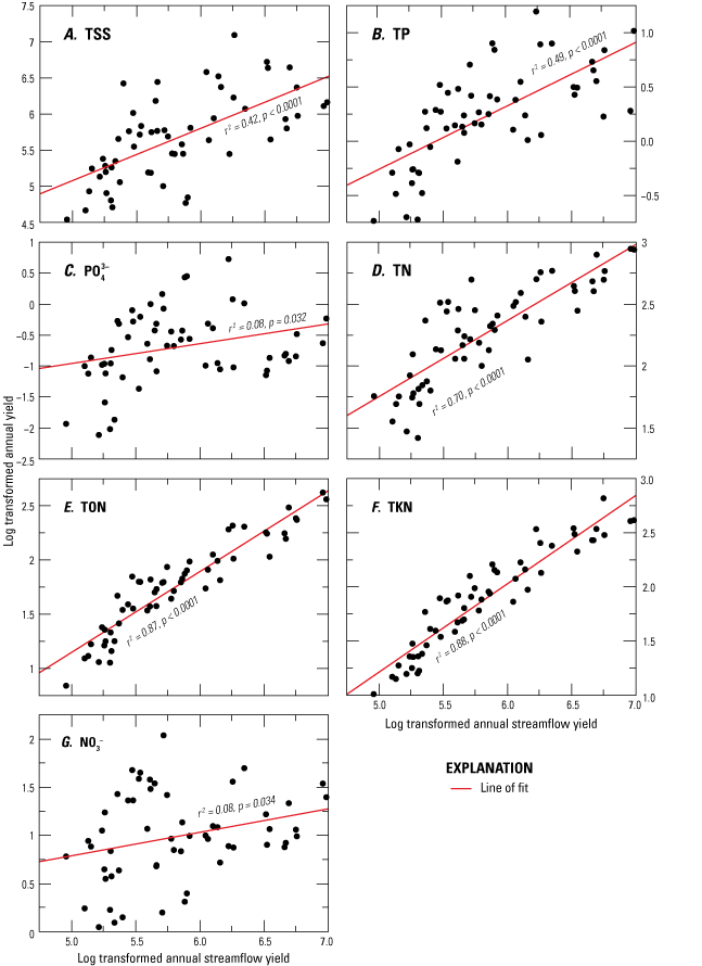
Annual streamflow yields plotted against annual yields of, A, total suspended solids (TSS), B, total phosphorus (TP), C, orthophosphate (PO43-), D, total nitrogen (TN), E, total organic nitrogen (TON), F, total Kjeldahl nitrogen (TKN), and G, nitrate plus nitrite (NO3-) with line of fit, correlation coefficient (r2), and p-value.
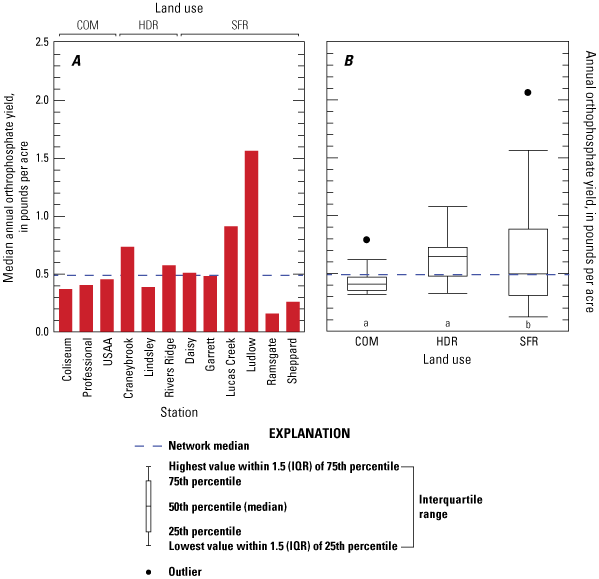
Orthophosphate yields presented as, A, a bar plot of the median annual total from water year 2016 through 2020 at each of the 12 monitoring stations, and, B, boxplots of annual yields grouped by land use over the same period. A water year begins October 1 and ends September 30. Non-matching letters denote statistical significance based on p less than or equal to 0.05. Station names are defined as Coliseum, Storm Drain at Coliseum Drive at Hampton, Virginia (Va.); Professional, Storm Drain at Professional Place near Chesapeake, Va.; Storm Drain at USAA Drive at Norfolk, Va.; Craneybrook, Storm Drain at Craneybrook Lane at Edgefield, Va.; Lindsley, Storm Drain at Lindsley Drive near Virginia Beach, Va.; Rivers Ridge, Storm Drain at Rivers Ridge Circle near Newport News, Va.; Daisy, Storm Drain at Daisy Drive near Portsmouth, Va.; Garrett, Storm Drain West of Garrett Drive at Hampton, Va.; Lucas Creek, Storm Drain at Lakewood Park Drive near Newport News, Va.; Ludlow, Storm Drain at Ludlow Drive near Kempsville, Va.; Ramsgate, Conveyance Channel at Ramsgate Lane near Great Bridge, Va.; Sheppard, Storm Drain at Sheppard Avenue near Norfolk, Va. Stations are arranged by land use.
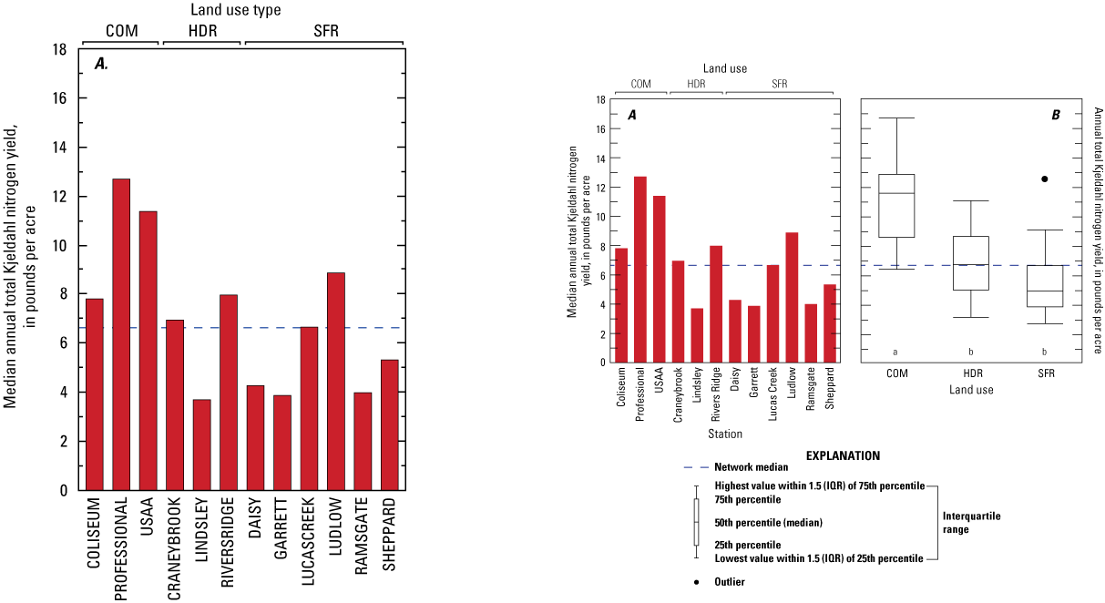
A, Total Kjeldahl nitrogen concentrations at the 12 monitoring stations and B, across 3 land-use types for water years 2016 through 2020. A water year begins October 1 and ends September 30. Non-matching letters indicate statistically significant differences in concentration between land-use types. Significance is based on p less than for equal to 0.05. Station names are defined as Coliseum, Storm Drain at Coliseum Drive at Hampton, Virginia (Va.); Professional, Storm Drain at Professional Place near Chesapeake, Va.; USAA, Storm Drain at USAA Drive at Norfolk, Va.; Craneybrook, Storm Drain at Craneybrook Lane at Edgefield, Va.; Lindsley, Storm Drain at Lindsley Drive near Virginia Beach, Va.; Rivers Ridge, Storm Drain at Rivers Ridge Circle near Newport News, Va.; Daisy, Storm Drain at Daisy Drive near Portsmouth, Va.; Garrett, Storm Drain West of Garrett Drive at Hampton, Va.; Lucas Creek, Storm Drain at Lakewood Park Drive near Newport News, Va.; Ludlow, Storm Drain at Ludlow Drive near Kempsville, Va.; Ramsgate, Conveyance Channel at Ramsgate Lane near Great Bridge, Va.; Sheppard, Storm Drain at Sheppard Avenue near Norfolk, Va. Stations are arranged by land use.
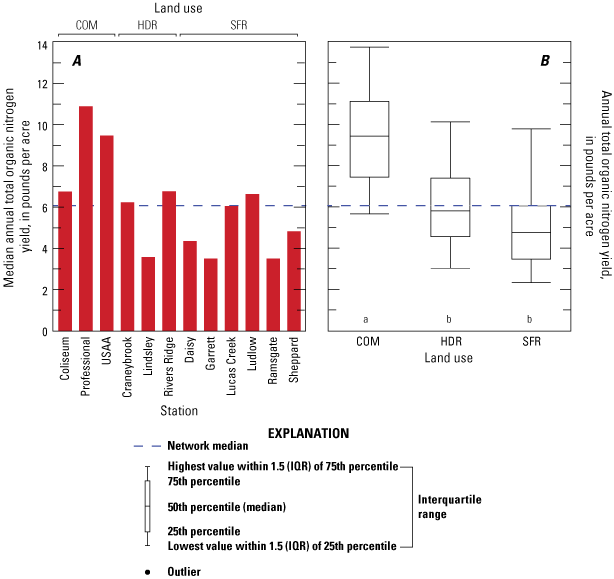
A, Total organic nitrogen concentrations at the 12 monitoring stations and B, across 3 land-use types for water year 2016 through 2020. A water year begins October 1 and ends September 30. Non-matching letters indicate statistically significant differences in concentration between land-use types. Significance is based on p less than or equal to 0.05. Station names are defined as Coliseum, Storm Drain at Coliseum Drive at Hampton, Virginia (Va.); Professional, Storm Drain at Professional Place near Chesapeake, Va.; USAA, Storm Drain at USAA Drive at Norfolk, Va.; Craneybrook, Storm Drain at Craneybrook Lane at Edgefield, Va.; Lindsley, Storm Drain at Lindsley Drive near Virginia Beach, Va.; Rivers Ridge, Storm Drain at Rivers Ridge Circle near Newport News, Va.; Daisy, Storm Drain at Daisy Drive near Portsmouth, Va.; Garrett, Storm Drain West of Garrett Drive at Hampton, Va.; Lucas Creek, Storm Drain at Lakewood Park Drive near Newport News, Va.; Ludlow, Storm Drain at Ludlow Drive near Kempsville, Va.; Ramsgate, Conveyance Channel at Ramsgate Lane near Great Bridge, Va.; Sheppard, Storm Drain at Sheppard Avenue near Norfolk, Va. Stations are arranged by land use.
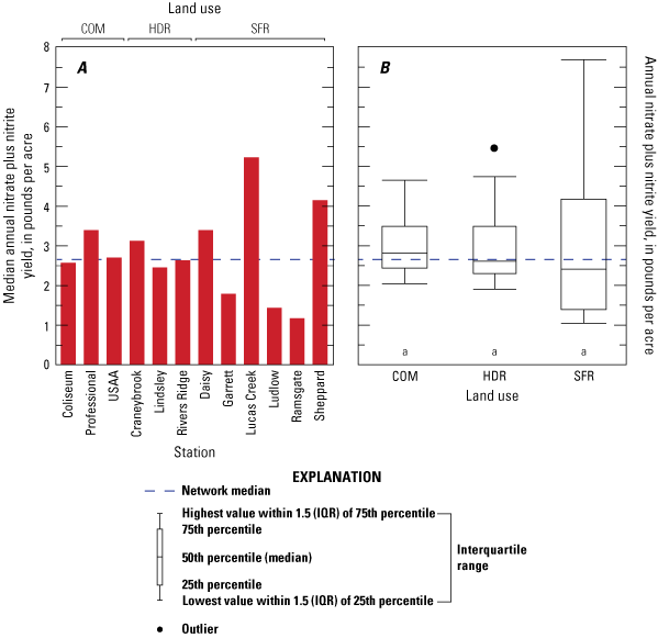
A, Nitrate plus nitrite concentrations at the 12 monitoring stations and B, across 3 land-use types for water years 2016 through 2020. A water year begins October 1 and ends September 30. Non-matching letters indicate statistically significant differences in concentration between land-use types. Significance is based on p less than or equal to 0.05. Coliseum, Storm Drain at Coliseum Drive at Hampton, Virginia (Va.); Professional, Storm Drain at Professional Place near Chesapeake, Va.; USAA, Storm Drain at USAA Drive at Norfolk, Va.; Craneybrook, Storm Drain at Craneybrook Lane at Edgefield, Va.; Lindsley, Storm Drain at Lindsley Drive near Virginia Beach, Va.; Rivers Ridge, Storm Drain at Rivers Ridge Circle near Newport News, Va.; Daisy, Storm Drain at Daisy Drive near Portsmouth, Va.; Garrett, Storm Drain West of Garrett Drive at Hampton, Va.; Lucas Creek, Storm Drain at Lakewood Park Drive near Newport News, Va.; Ludlow, Storm Drain at Ludlow Drive near Kempsville, Va.; Ramsgate, Conveyance Channel at Ramsgate Lane near Great Bridge, Va.; Sheppard, Storm Drain at Sheppard Avenue near Norfolk, Va. Stations are arranged by land use.
Conversion Factors
U.S. customary units to International System of Units
| Multiply | By | To obtain |
|---|---|---|
| inch (in.) | 2.54 | centimeter (cm) |
| inch (in.) | 25.4 | millimeter (mm) |
| foot (ft) | 0.3048 | meter (m) |
| acre | 4,047 | square meter (m2) |
| acre | 0.4047 | hectare (ha) |
| acre | 0.004047 | square kilometer (km2) |
| square mile (mi2) | 2.590 | square kilometer (km2) |
| cubic foot (ft3) | 0.02832 | cubic meter (m3) |
| foot per second (ft/s) | 0.3048 | meter per second (m/s) |
| cubic foot per acre (ft3/acre) | 0.0699725 | cubic meter per hectare (m3/ha) |
| cubic foot per acre per hour ([ft3/acre]/hour) | 0.0699725 | cubic meter per hectare per hour ([m3/ha]/hour) |
| cubic foot per second (ft3/s) | 0.02832 | cubic meter per second (m3/s) |
| cubic foot per second per square mile ([ft3/s]/mi2) | 0.01093 | cubic meter per second per square kilometer ([m3/s]/km2) |
| cubic foot per day (ft3/d) | 0.02832 | cubic meter per day (m3/d) |
| pound, avoirdupois (lb) | 0.4536 | kilogram (kg) |
| ton, short (2,000 lb) | 0.9072 | metric ton (t) |
| pound per acre per year ([lb/acre]/yr) | 1.121 | kilogram per hectare per year ([kg/ha]/yr) |
| pound per acre (lbs/acre) | 1.121 | kilogram per hectare (kg/ha) |
International System of Units to U.S. customary units
| Multiply | By | To obtain |
|---|---|---|
| centimeter (cm) | 0.3937 | inch (in.) |
| millimeter (mm) | 0.03937 | inch (in.) |
| meter (m) | 3.281 | foot (ft) |
| kilometer (km) | 0.6214 | mile (mi) |
| square meter (m2) | 0.0002471 | acre |
| square kilometer (km2) | 247.1 | acre |
| square meter (m2) | 10.76 | square foot (ft2) |
| square kilometer (km2) | 0.3861 | square mile (mi2) |
| cubic meter (m3) | 35.31 | cubic foot (ft3) |
| meter per second (m/s) | 3.281 | foot per second (ft/s) |
| meter per year (m/yr) | 3.281 | foot per year (ft/yr) |
| cubic meter per hectare (m3/ha) | 14.2913 | cubic foot per acre (ft3/acre) |
| cubic meter per hectare per hour (m3/ha/hour) | 14.2913 | cubic foot per acre per hour (ft3/acre/hour) |
| cubic meter per second (m3/s) | 35.31 | cubic foot per second (ft3/s) |
| cubic meter per second per square kilometer ([m3/s]/km2) | 91.49 | cubic foot per second per square mile ([ft3/s]/mi2) |
| cubic meter per day (m3/d) | 35.31 | cubic foot per day (ft3/d) |
| kilogram (kg) | 2.205 | pound avoirdupois (lb) |
| metric ton (t) | 1.102 | ton, short [2,000 lb] |
| kilogram per hectare per year ([kg/ha]/yr) | 0.8921 | pound per acre per year ([lb/acre]/yr) |
| kilogram per hectare (kg/yr) | 0.8921 | pound per acre (lb/acre) |
Temperature in degrees Celsius (°C) may be converted to degrees Fahrenheit (°F) as follows:
°F = (1.8 × °C) + 32.
Temperature in degrees Fahrenheit (°F) may be converted to degrees Celsius (°C) as follows:
°C = (°F – 32) / 1.8.
Datum
Horizontal coordinate information is referenced to the North American Datum of 1983 (NAD 83).
Altitude, as used in this report, refers to distance above the vertical datum.
Supplemental Information
Specific conductance is given in microsiemens per centimeter at 25 degrees Celsius (µS/cm at 25 °C).
Concentrations of chemical constituents in water are given in milligrams per liter (mg/L)
Abbreviations
AMLE
adjusted maximum likelihood estimation
BFI
base-flow index
BMP
best management practice
CB-NTN
Chesapeake Bay Non-tidal Network
CBWM
Chesapeake Bay Watershed Model
COM
commercial
EPA
U.S. Environmental Protection Agency
HDR
high-density residential
HRPDC
Hampton Roads Planning District Commission
HRSD
Hampton Roads Sanitation District
MDL
method detection limit
MS4
municipal separate storm sewer systems
N
nitrogen
NH3
ammonia plus ammonium
NO3-
nitrate plus nitrite
NPS
nonpoint source
NSQD
National Stormwater Quality Database
NWIS
National Water Information System
P
phosphorus
PC
principal components
PO43-
orthophosphate
PP
Physiographic Province
r
Pearson’s correlation coefficient
RBI
Richards-Baker flashiness index
SC
specific conductance
SFR
single-family residential
TB
turbidity
TKN
total Kjeldahl nitrogen
TMDL
total maximum daily load
TN
total nitrogen
TON
total organic nitrogen
TP
total phosphorus
TSS
total suspended solids
USGS
U.S. Geological Survey
WT
water temperature
WY
water year (water years begin October 1 and end September 30 of the following year)
For more information, contact
Center Director, Virginia and West Virginia Water Science Center
U.S. Geological Survey
1730 East Parham Road, Richmond, VA 23228
Publishing support provided by the West Trenton Publishing Service Center.
Disclaimers
Any use of trade, firm, or product names is for descriptive purposes only and does not imply endorsement by the U.S. Government.
Although this information product, for the most part, is in the public domain, it also may contain copyrighted materials as noted in the text. Permission to reproduce copyrighted items must be secured from the copyright owner.
Suggested Citation
Porter, A.J., 2022, Stormwater quantity and quality in selected urban watersheds in Hampton Roads, Virginia, 2016–2020: U.S. Geological Survey Scientific Investigations Report 2022–5111, 77 p., https://doi.org/10.3133/sir20225111.
ISSN: 2328-0328 (online)
ISSN: 2328-031X (print)
Study Area
| Publication type | Report |
|---|---|
| Publication Subtype | USGS Numbered Series |
| Title | Stormwater quantity and quality in selected urban watersheds in Hampton Roads, Virginia, 2016–2020 |
| Series title | Scientific Investigations Report |
| Series number | 2022-5111 |
| ISBN | 978-1-4113-4488-4 |
| DOI | 10.3133/sir20225111 |
| Publication Date | November 23, 2022 |
| Year Published | 2022 |
| Language | English |
| Publisher | U.S. Geological Survey |
| Publisher location | Reston, VA |
| Contributing office(s) | Virginia and West Virginia Water Science Center |
| Description | Report: xi, 77 p.; Data Release |
| Country | United States |
| State | Virginia |
| City | Hampton Roads |
| Online Only (Y/N) | N |
| Additional Online Files (Y/N) | N |