

Hydrologic Change in the St. Louis River Basin from Iron Mining on the Mesabi Iron Range, Northeastern Minnesota
Links
- Document: Report (18.2 MB pdf) , HTML , XML
- Data Releases:
- USGS data release —MODFLOW–NWT simulations of regional groundwater flow under mining and pre-mining scenarios near the Mesabi Iron Range within the St. Louis River Basin, northeastern Minnesota
- USGS data release —Soil-water-balance model data sets for the St. Louis River drainage basin, northeast Minnesota, 1995–2010
- Download citation as: RIS | Dublin Core
Acknowledgments
The U.S. Environmental Protection Agency’s Great Lakes Restoration Initiative funded this project. Funds were acquired by a partnership coordinated by Nancy Schuldt, the Water Projects Coordinator of the Fond du Lac Band of the Minnesota Chippewa Tribe. Partners include the Fond du Lac Band of Lake Superior Chippewa, the Bois Forte Band of Chippewa, the Mille Lacs Band of Ojibwe, and the Leech Lake Band of Ojibwe, all of the Minnesota Chippewa Tribe, the Great Lakes Indian Fish & Wildlife Commission, the Minnesota Pollution Control Agency, and the U.S. Geological Survey Cooperative Water Program. We thank Andy Leaf of the U.S. Geological Survey for producing the U.S. Geological Survey Modular Three-dimensional Finite-Difference Ground-water Flow model (MODFLOW) Streamflow Routing (SFR2) input file for the groundwater models documented in this report.
All authors were involved in the production of the models documented in this report. Each author led parts of the model design, production, calibration, results analysis, report writing, and project management. Timothy (Tim) Cowdery was responsible for project management, flow model geologic and hydrologic conceptualization, and model-results analysis leadership. He also designed and produced the report figures and tables. Anna Baker aggregated, analyzed, and produced much of the geographic information system and head calibration data. She designed and led the base flow synoptic measurement, assisted by Megan (Meg) Haserodt. Meg Haserodt compiled streamflow data and produced base flow separations. Daniel Feinstein, Meg Haserodt, and Randall (Randy) Hunt designed approaches to representing hydrologic features in the models and the model grids. Daniel Feinstein and Meg Haserodt produced the MODFLOW input files. Daniel Feinstein wrote the model output programs used in model calibration and output analysis. Randy Hunt designed and executed the automated parameter-estimation software (PEST) calibration for the mining model. Tim Cowdery and Anna Baker wrote the first report draft of the manuscript, and Tim incorporated revisions. All authors commented on the draft and approved the final manuscript.
Abstract
This study compares the results of two regional steady-state U.S. Geological Survey Modular Three-Dimensional Finite-Difference Ground-Water Flow (MODFLOW) models constructed to quantify the hydrologic changes in the St. Louis River Basin from iron mining on the Mesabi Iron Range in northeastern Minnesota. The U.S. Geological Survey collaborated in this study with bands of the Minnesota Chippewa Tribe, and the Minnesota Pollution Control Agency to inform management decisions about aquatic resources in the St. Louis River Basin. A model constructed and calibrated to represent average 1995–2015 mining conditions produced regional groundwater heads and flows. A pre-mining scenario model was constructed from this mining model but had the land and bedrock surfaces restored to pre-mining topographies and had modeled mining features (mine pits, tailings basins, waste-rock piles, and mining-disturbed areas) eliminated to represent general pre-mining stratigraphy and hydrogeology. Many of the features important to the hydrology of this mining area (like individual mine pits) are difficult to represent in groundwater models and required the use of modeling tools to indirectly account for their effects. The difference between the results of these two models represents mining’s effects on the hydrology in the Mesabi Iron Range area of the St Louis River Basin. The mining and pre-mining regional models also can provide boundary conditions and initial properties for future local or site-specific groundwater-flow models in the area.
Total groundwater flow through the mining model is 171 million cubic feet per day. Areal recharge is the largest source of groundwater (78 and 81 percent of total groundwater flow in the mining and pre-mining scenario models, respectively). Seepage from streams and lakes provides another 17 percent of the total groundwater flow through both models. Water leaves aquifers through seepage to streams (discharge as base flow, 43 percent in both models) and areal seepage to the land surface (surface seepage), for example to wetlands (45 and 49 percent, mining and pre-mining scenario models respectively).
Comparison of the results from the mining and pre-mining scenario models shows that iron mining has produced measurable hydrologic changes in the St. Louis River Basin, but that most of those changes and the highest magnitude changes occur near the mining features. Flow changes to and from surface-water bodies like streams and wetlands were analyzed in detail because of their importance in sustaining surface waters and aquatic life. Overall, groundwater flow in the mining model was 3.62 million cubic feet per day (2.2 percent) greater than total pre-mining model groundwater flow. This was caused by an increase in recharge from tailings basins and a decrease in discharge from surface seepage. Groundwater discharge to mine pits was the largest change in groundwater flows between the models (a change representing 2.8 percent of total pre-mining model groundwater flow). Net recharge to groundwater from tailings basins (2.4 percent), net decrease in surface seepage from groundwater (2.7 percent), and net increase in seepage to streams (1.0 percent) were all in this same range of total pre-mining model groundwater flow. Groundwater lost through mine-pit withdrawals was nearly offset by groundwater gained through recharge from tailings basins. However, because losses and gains occurred in different areas, the effect of mining can have more substantial effects on local areas than the model-wide averages represent.
Introduction
Iron has been mined in and adjacent to the St. Louis River Basin in northeastern Minnesota for more than a century. Iron mining is concentrated along the northern border of the Basin. Some effects of mining are obvious and can be substantial near the mines (Lively and others, 2002; Berndt and Bavin, 2009; Tetra Tech, 2014). For example, mining can remove aquifer material and expose otherwise buried confined aquifers at the land surface. During mining and after it ceases, mines, waste-rock piles, and tailings basins can continue to affect the hydrology. Removing water from mine pits or underground mines can cause hydrologic changes near the mines, such as changes in groundwater-flow directions and rates, changes in the area of surface-water or groundwater basins, and changes in stream base flow. Streamflow may increase from water discharged to rivers to dewater mines or it may decrease because dewatering can divert discharge to other surface waters. But groundwater and surface-water flows can increase and decrease in complex ways from mining and the aggregate hydrologic effect of the changes associated with mining in the St. Louis River is not well understood.
The Reservation of the Fond du Lac Band of Lake Superior Chippewa of the Minnesota Chippewa Tribe (FDLB) is in the southern part of the St. Louis River Basin, 50 miles (mi) south of the city of Virginia and 25 mi west of the city of Duluth (inset map, fig. 1), in northeastern Minnesota. The reservation is bordered on the north and east by the St. Louis River. FDLB tribal members rely on natural resources upstream from the 157-square-mile (mi2) reservation. All Minnesota Chippewa (Ojibwe) Tribe members rely on resources guaranteed by treaty outside reservations throughout much of the rest of the St. Louis River Basin. Effective stewardship requires that tribal resource managers understand the St. Louis River’s original hydrology and how mining and other land-use changes in the St. Louis River Basin have altered it (Tetra Tech, 2014). The understanding now does not meet the need.
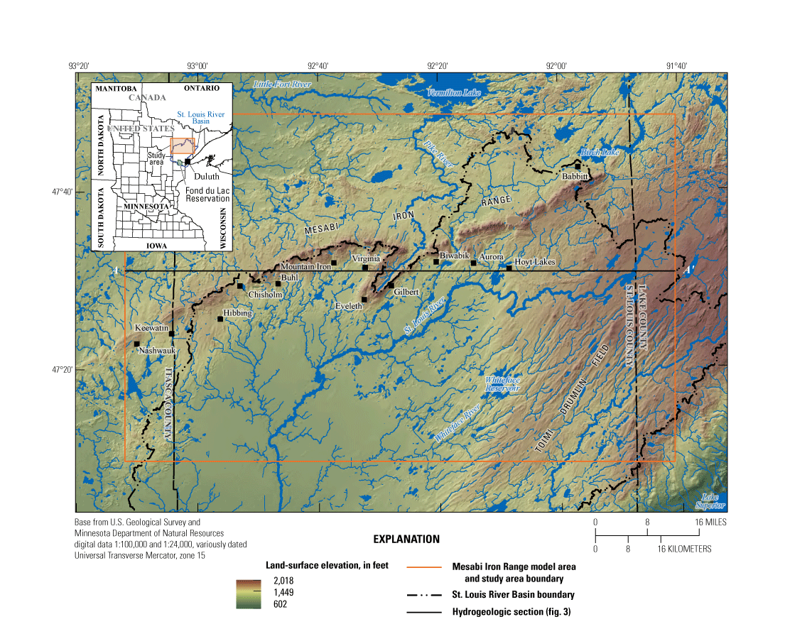
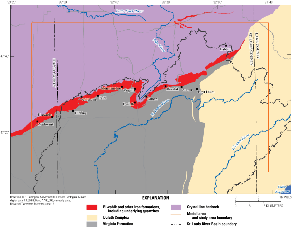
Topography and location of the Mesabi Iron Range and the study area, northeastern Minnesota.
To address the lack of hydrologic information, bands of the Minnesota Chippewa Tribe partnered with the U.S. Geological Survey (USGS) to pursue a two-phase groundwater modeling study of the St. Louis River Basin. The first phase produced a simulation of two-dimensional regional groundwater flow for the entire St. Louis River Basin (Haserodt, and others, 2019). The second phase examined the effects of iron mining (including present iron mining) on groundwater flow in the historical mining area of the Mesabi Iron Range (fig. 1) and on base flow to the St. Louis River and its tributaries. The approach of the second study phase, documented in this report, was to compare results of a groundwater-flow model of recent (1995–2015) mined conditions (hereinafter, mining model) with the results of a pre-mining scenario model (hereinafter, pre-mining model). This report discusses the (1) conceptual model of groundwater flow in the study area; (2) the three-dimensional modeling method; (3) the development, calibration, and results of the mining model; (4) the development and results of the pre-mining model; (5) the assumptions and limitations of the two models; and (6) the hydrologic differences between the two models.
Purpose and Scope
The objective of this study is to investigate the cumulative effects of mining on groundwater and stream base flow in the St. Louis River Basin by simulating groundwater flow. Steady-state finite-difference models of groundwater flow were produced, considering groundwater and surface water in the Basin as a single interconnected resource. The study accomplishes two objectives:
-
describes the general distribution, direction, and rate of groundwater flow and groundwater-surface water interactions across the northern St. Louis River Basin between the Mesabi Iron Range and St. Louis River (fig. 1), and
-
evaluates the cumulative hydrologic effects of iron mining in the study area.
Geology, Groundwater Flow, and Interaction with Surface Waters
Haserodt and others (2019) provide a description of the St. Louis River Basin hydrogeologic setting and a conceptual model of its groundwater flow. The following is a condensation of that discussion with emphasis on the study area and groundwater flows to the St. Louis River and its tributaries in that area. The study area comprises 3,205 mi2 in the northern half of the St. Louis River Basin. About 60 percent of the study area is within this Basin. The remaining 40 percent is within the Rainy River Basin to the north and Mississippi River Basin to the west. The Mesabi Iron Range (hereinafter, Iron Range) forms the divide between the St. Louis River Basin and every other basin in the region except for the Embarrass River Basin, a tributary to the St. Louis River, whose headwaters are north of the Iron Range. Lakes and wetlands are common within the study area. Parts of the basins of two major tributaries to the St. Louis River, the Cloquet and the Whiteface, are partly within the study area, but these tributaries do not contribute flow to the St. Louis River inside of the study area.
The Iron Range is the topographically high area in the northern part of the study area. The Toimi Drumlin Field is the topographically high area in the southeast part of the study area (fig. 1). The headwaters and main channel of the St. Louis River lie between these two highlands. Much of this lower part of the river basin within the study area is quite flat, containing extensive areas of lakes and wetlands. Many of these wetlands were drained for agriculture in the first two decades of the 20th century, especially in the southwest part of the study area (King, 1980). Topography and hydrology have been substantially altered by iron mining along the Iron Range. Much of the area in the northwest third of the study area is covered with thin (less than 50 feet [ft]) glacial sediments (fig. 2). Note that the discontinuity of thickness data along a north-south line through the town of Aurora in figure 2 is the result of combining different datasets from the Minnesota Geologic Survey (MGS; M. Jirsa, MGS, written commun., January 30, 2018; Jirsa and others, 2010; Jirsa, 2016) to produce a study-area-wide coverage.
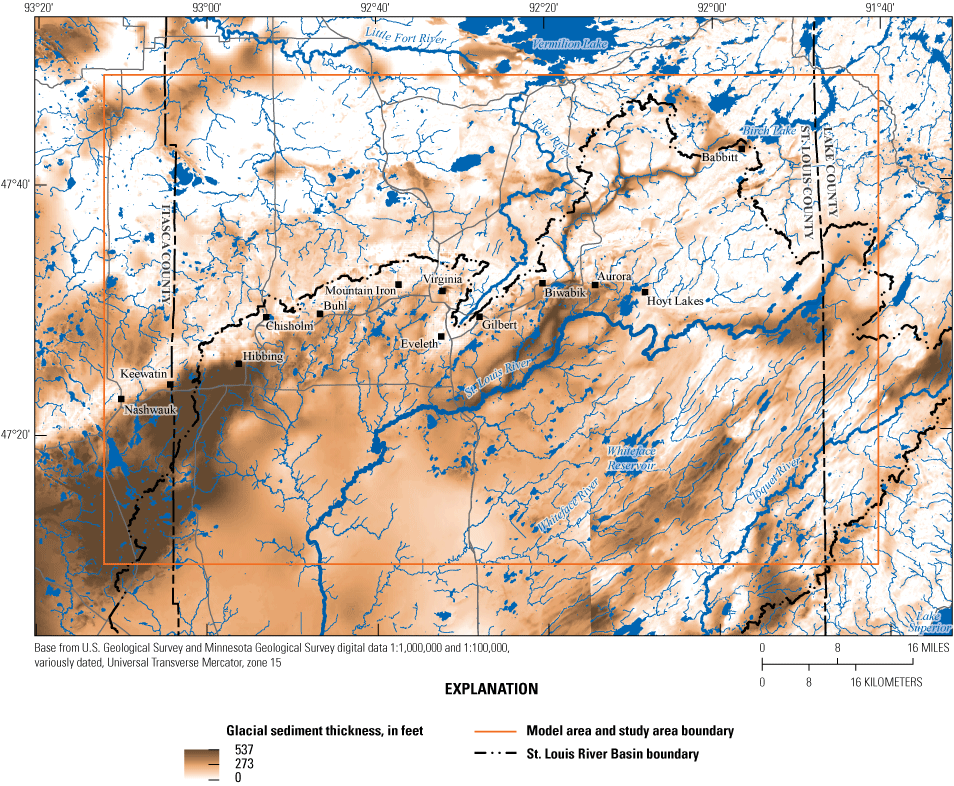
Thickness of glacial sediments in the study area, northeastern Minnesota.
The conceptual understanding of study area aquifers and groundwater flow within them is based on the geologic and hydrologic studies detailed in Haserodt and others (2019). Results of this 2019 study show that basin-scale groundwater flow is generally to the south and southwest within the St. Louis River Basin. Groundwater discharges to streams, lakes, wetlands, reservoirs, and the land surface in areas where groundwater head in the aquifers is higher than surface-water levels or the land surface. These discharges help keep rivers in the basin flowing during nonrain periods. Some wetlands in the basin are not connected to the St. Louis River stream network except during wet periods. Most of the groundwater that discharges to these disconnected wetlands likely leaves the basin through evapotranspiration (ET; Cowdery and others, 2019).
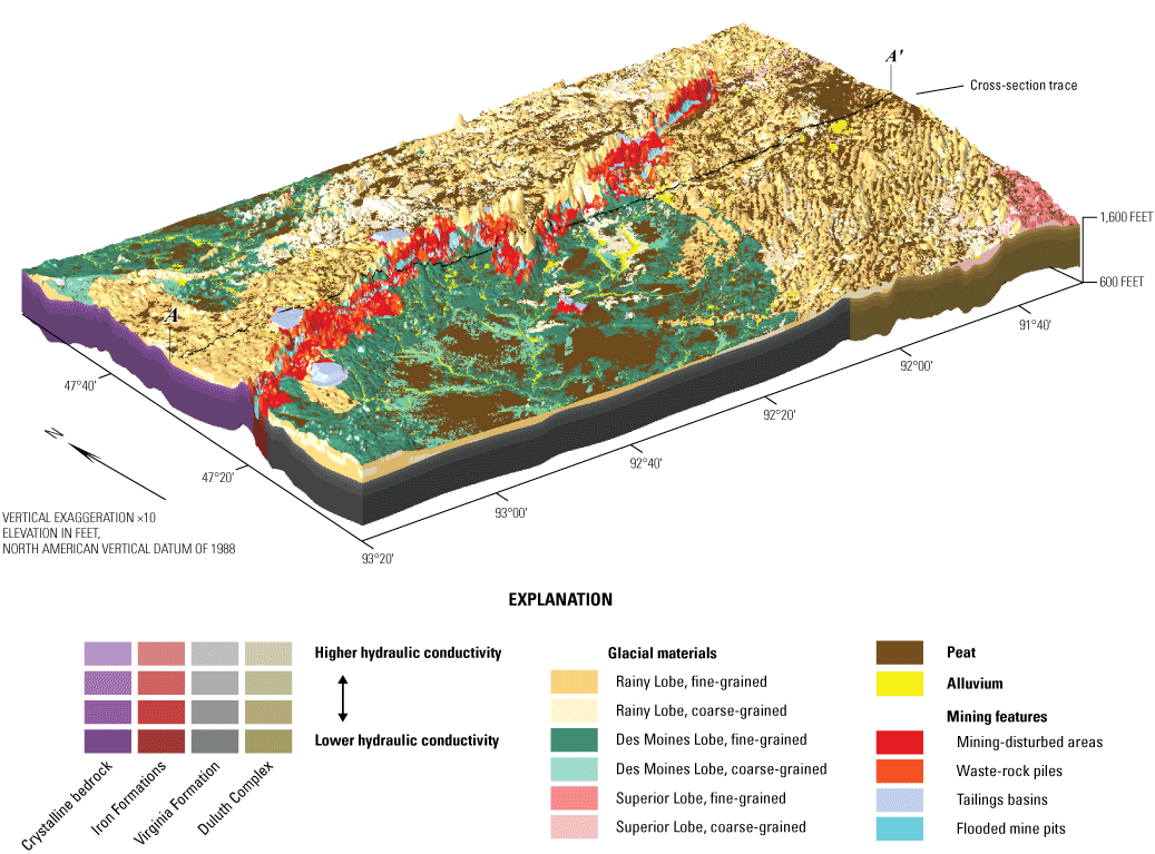
In general, more groundwater discharges to the surface from shallow and higher conductivity aquifers than from deeper and lower conductivity aquifers. St. Louis River Basin aquifers exist either in glacial deposits or in fractured bedrock. (fig. 3). Bedrock is exposed at land surface in very small areas of the basin near the Iron Range.
Aquifer relations in the study area, northeastern Minnesota.
Glacial Aquifers
Glacial aquifers are genetically complex and spatially heterogeneous sand and gravel bodies upon, within, and under finer-grained glacial tills and lake clays. However, some tills are hydraulically conductive enough to contribute water to sand and gravel. Surficial glacial aquifers are exposed at the land surface. Areal recharge rates tend to be highest in surficial glacial aquifers because they are coarse grained (have higher hydraulic conductivity) and receive infiltrating water directly at land surface. Where surface waters (streams, lakes, and wetlands) lie in direct contact with surficial glacial aquifers, which is common in the study area, the water table is shallow and water exchanges easily between groundwater and surface water. Groundwater usually discharges to surface waters, which tend to lie low in the landscape. The areal extent and, to a lesser degree, thickness of surficial glacial aquifers is quite well known in the study area (figs. 2 and 4). Meltwaters of three different glacial lobes of the Laurentide Ice Sheet deposited the areally extensive surficial glacial aquifer sediments in the study area: the Rainy Lobe, the Superior Lobe, and St. Louis Sublobe of the Des Moines Lobe (glacial-lobe areas on fig. 4). Surficial aquifers deposited by the Rainy Lobe cover much of the study area. Aquifers formed of Superior Lobe deposits lie in the southeast part of the study area (fig. 4). Aquifers composed of St. Louis Sublobe deposits form a thin veneer throughout the southwest, central, and northwest parts of the study area. Although the tills deposited by these lobes are different (Johnson and others, 2016), the sands and gravels that compose these aquifers are similar because the depositional processes are similar among these ice lobes.
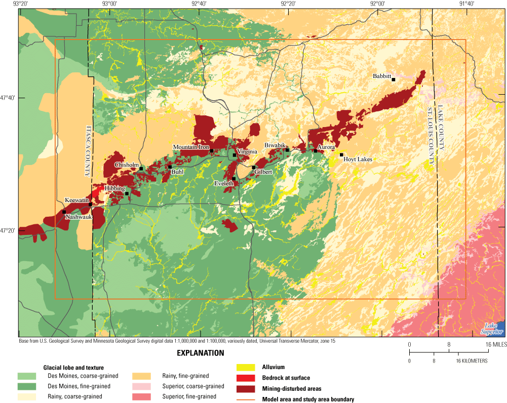
Simplified surficial glacial geology of the study area, northeastern Minnesota.
Buried glacial aquifers are sands and gravels deposited within or beneath relatively fine-grained glacial tills or lake clays. Some buried glacial aquifers may be partly in contact with underlying bedrock or with overlying surficial glacial aquifers. In general, however, fine-grained sediments form confining beds around the buried glacial aquifers. Compositionally, hydraulically, and genetically, buried glacial aquifers are similar to surficial ones. However, each buried glacial aquifer was formed by more than one glacial advance: first, at least one advance that deposited coarse-grained sediment that was followed by at least one advance that deposited fine-grained sediment. This process, through successive glacial advances, produced buried glacial aquifers that are generally less areally extensive than surficial ones. The extent of buried glacial aquifers in the study area is much less well known than the extent of surficial glacial aquifers because the only information about them comes from boreholes.
Buried glacial aquifers are recharged by leakage of water from the materials that surround them. Tills, lake clays, and bedrock are generally much less hydraulically conductive than is the sand and gravel of aquifers (Fetter, 2000), so flow within buried glacial aquifers is controlled by the hydraulic properties of the fine-grained materials surrounding them. If buried glacial aquifers are connected to surficial glacial aquifers, however, flow can be controlled by the area of that connection. Pumping from a buried glacial aquifer can increase the rate of flow through it by increasing the groundwater-head gradients toward the well.
Bedrock Aquifers
Geologists have divided the bedrock in the St. Louis River Basin into scores of rock types (Haserodt, and others, 2019, p. 3 and the citations therein). These rocks are old (Middle Precambrian or older), hard, dense, and fractured at the surface. In general, because the density of fractures in bedrock decreases with depth, so too will its hydraulic conductivity (Haserodt and others, 2019, p. 3). For the purpose of groundwater flow, bedrock in the study area can be aggregated into four hydrostratigraphic groups (fig. 5):
-
crystalline bedrock comprising granites, metamorphosed volcanic rocks, and metamorphosed sediments like slates and quartzites;
-
the Biwabik Iron Formation comprising metamorphosed iron-rich near-shore sediments that include the underlying thin, genetically related Pokegama Quartzite. Other small iron formations on the northern border of the study area (fig. 5) are lumped together with the surrounding crystalline bedrock in this study;
-
the Virginia formation (Morey, 1972) graywackes (with some argillites); and
-
the Duluth Complex comprising layered intrusive gabbroic rocks.
Simplified bedrock geology of the study area, northeastern Minnesota.
These groups are based on age, depositional environment, contiguity, mapping scale, rocks of interest to the study, and presumed similarity of rock hydrologic properties. Except for the Biwabik Iron Formation, water likely travels primarily, if not exclusively, through fractures in these bedrock groups because these rock types are not porous. At some depth, fractures in bedrock become so small and infrequent that nonvuggy bedrock becomes effectively impermeable. In the Biwabik Iron Formation, water can also travel through interconnected voids in the rock matrix, known as vugs. The existence of vugs in these rocks varies greatly, spatially (Siegel and Ericson, 1980). A literature review by Haserodt and others (2019) found that the hydraulic conductivity of these bedrock groups generally increases in this order: Duluth Complex, crystalline bedrock, Virginia formation, and Biwabik Iron Formation. However, where the Biwabik Iron Formation is not very vuggy, it can have much lower hydraulic conductivity.
The Virginal Formation was deposited on the Biwabik Iron formation which was deposited on crystalline bedrock. The contacts of these three bedrock groups dip to the southeast toward the Lake Superior Basin at an angle of about 5–15 degrees (Morey, 1972). The contact between the Duluth Complex and the graywackes of the Virginia formation is poorly known areally, interfingered, complex, and variable (Bonnichsen, 1972). In this work, the contacts between the Duluth Complex and other bedrock groups are assumed to be roughly vertical in the absence of better information. In most places in the study area, bedrock aquifers are buried beneath glacial deposits. Where these deposits are thin (fig. 2) or coarse-grained, bedrock aquifers may be locally unconfined. But generally, bedrock aquifers are confined by glacial tills or lake clays of varying hydraulic conductivities; Superior Lobe has the sandiest and most conductive till, and the St. Louis Sublobe has the most clay-rich and least conductive till (Johnson and others, 2016). Lake clays are the least conductive of all the glacial sediments. St. Louis Sublobe tills and all lake clays are so clay rich that most groundwater moves through fractures within these sediments. The aperture of these fractures closes with depth (McKay and others, 1993), meaning that hydraulic conductivity of these clayey materials decreases with depth.
Mining Groundwater-Flow Model
Horizontal and vertical groundwater flow and groundwater head within the current mined landscape in the study area of the St. Louis River Basin is calculated by the mining model. This model area is affected by more than 100 years of mining and associated changes in the landscape. The model is executed using the U.S. Geological Survey Modular Three-dimensional Finite-Difference Ground-water Flow model (MODFLOW) computer program. This program uses a finite-difference scheme to solve the groundwater flow equations. The version used for models in this study is the MODFLOW–NWT code (Niswonger and others, 2011). The mining model incorporates complex hydrologic boundaries and stresses and quantifies groundwater fluxes to or from rivers, lakes, and wetlands. Because the model is steady state, imposed hydrologic stresses and results produced represent long-term average hydrologic conditions during the calibration period of 1995–2015.
The Iron Range model area (IRMA) is 3,205 mi2 in area and includes the part of the Iron Range within the St. Louis River Basin (fig. 1). This area is discretized into a MODFLOW model grid of 400-ft square cells composed of 594 rows and 940 columns, oriented with the cardinal directions. The model contains 558,360 cells per layer and is 8 layers thick with a total of 4,466,880 cells. This discretization was a compromise between a small cell size needed to simulate groundwater-surface water interaction and a larger cell size needed to make runtimes reasonable. The MODFLOW Newton-Raphson solver (Niswonger and others, 2011) was used because it handles dry cells (cells where the groundwater level is below the cell bottom) in the model more robustly than other MODFLOW solvers (Hunt and Feinstein, 2012)—a capability important for simulating wet and adjacent dry cells that occur near mine pits. An archive of all model input, output, executable, and ancillary files is available in a USGS ScienceBase model archive release (Cowdery and others, 2023).
The model was constructed to represent the hydrologically important features in the IRMA. In the next sections, we first describe how the model grid is discretized vertically to match the hydraulic-conductivity zones of the aquifers and confining layers. We then describe how the geology and some of the mining features of the IRMA were incorporated into hydraulic-conductivity zones in these layers. Next, we describe the techniques used to provide realistic water flows through the boundaries of the model. We then introduce the important hydrologic features (called hydrologic stresses) incorporated into the model and describe how we used the MODFLOW packages to represent them. These stresses include the features that represent mining in the model. Finally, we show how we used the MODFLOW Unsaturated-Zone Flow (UZF) package to determine where groundwater discharges to the land surface; areas interpreted as permanent wetlands in the model.
Model Layering
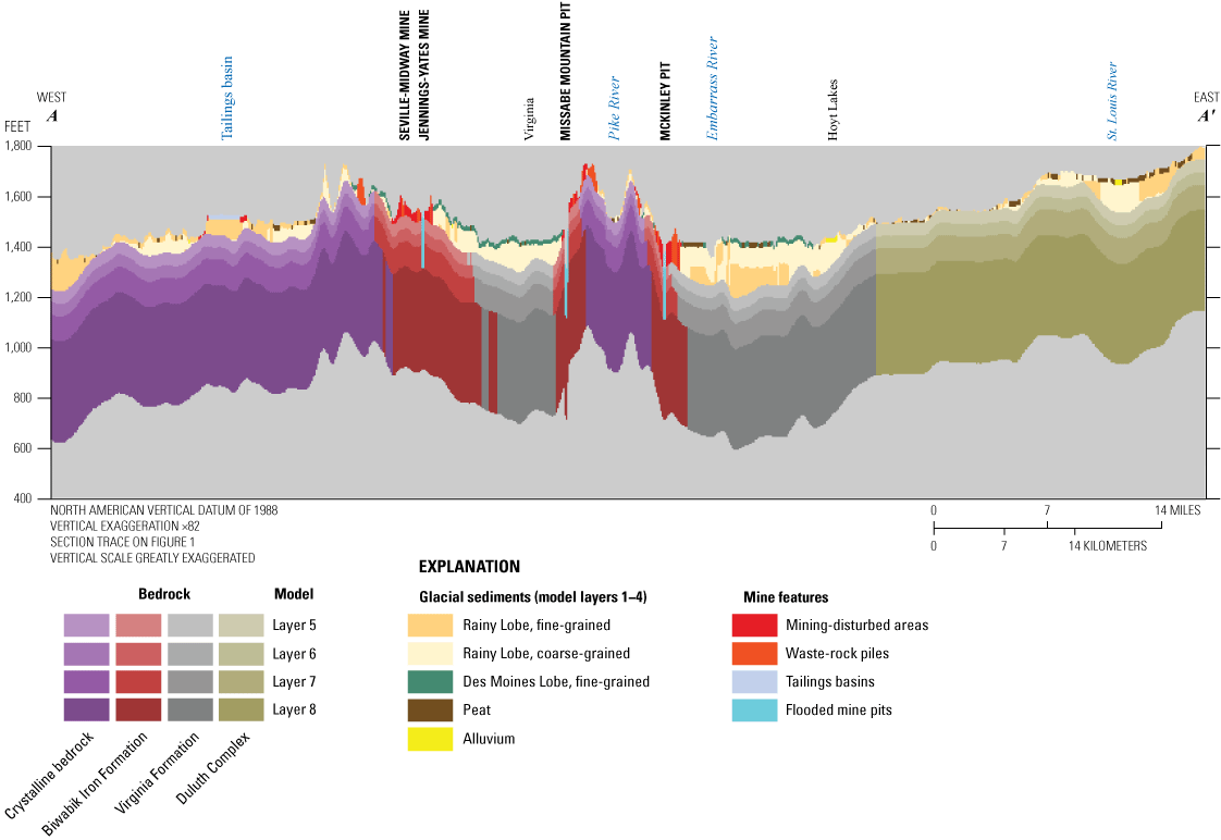
Model layers follow the land-surface and bedrock topography so that bedrock hydrostratigraphy can be realistically represented. The top of the model (layer 1) is the land surface generalized to the model grid from 1-meter (m) light detection and ranging (lidar) elevation data from the Minnesota Department of Natural Resources (MN–DNR, 2011). The upper four model layers (1–4) are parallel the land surface and represent glacial sediments (fig. 3) that are highly variable in thickness and composition (figs. 2 and 4) across the IRMA. These layers increase in thickness with depth (table 1) because available stratigraphic detail decreases with depth. The thickness of the layers is reduced to a minimum of 0.25 ft from layer 4 upward to layer 1 until the thickness of all four layers equals the thickness of the glacial sediments (fig. 3). However, in small areas where thick glacial sediments pinch out at land surface, minimum thickness of layers 1–4 is 0.01 ft. In this way, layers of glacial sediments were negligible where glacial deposits are thin or absent. The bottom four model layers (5–8; fig 3) represent bedrock. Each is assigned a constant thickness, paralleling the bedrock surface. The thicknesses of the layers increase with depth (table 1). This layering scheme allows hydraulic conductivity of bedrock to decrease with depth below the bedrock surface. The number and aperture of fractures in bedrock decrease with depth (M. Jirsa, MGS, oral communication, January 30, 2018), thereby decreasing the hydraulic conductivity with depth. The Biwabik Iron Formation dips through the entire thickness of the model at an angle to the bedrock and land surfaces. As a result, the Biwabik Iron Formation follows a stepped boundary vertically along the model grid (fig. 3). The overall thickness of the IRMA varies from 600.76 to 1103.49 ft across the IRMA.
Table 1.
Maximum model-layer thickness in the mining model, northeastern Minnesota.Model Surficial Geology
The basic surficial geology for layer one of the mining model was produced by combining data from the MGS’s Arrowhead mapping project (J. McDonald, MGS, written commun., 2019) in St. Louis and Lake Counties and MGS’s statewide Quaternary geology map (Hobbs and Goebel, 1982) in Itasca County. Glacial geology in the resulting map was generalized into areas of coarse sand and gravel and areas of fine sediment deposited by three glacial lobes: the Rainy Lobe, the St. Louis Sublobe of the Des Moines Lobe (Koochiching Lobe), and the Superior Lobe. Areas of peat accumulation and mining features from other sources were substituted for surficial geology where appropriate. The areas of peat accumulation were considered to be the areas of permanent wetlands in the IRMA. In St. Louis and Lake Counties, a separate map of peat areas from the MGS’s Arrowhead mapping project was substituted for surficial geology in model layer one. In Itasca County, the statewide Quaternary geology map does not contain information about glacial materials where peat is mapped. Glacial materials in these peat areas were interpolated from the trends of boundaries between surficial deposits outside of the peat areas to create a complete surficial material map. More accurate peat areas were then substituted for the surficial geology in model layer one in Itasca County. The more accurate peat map was created from the National Wetlands Inventory (NWI) map as modified by the MN–DNR to include information from spring aerial imagery collected during 2009–14 and ancillary data to improve wetland delineation and better support wetland management (MN–DNR, 2018). Areas of the MN–DNR modified NWI map with the following attributes were categorized as peat producing and therefore permanent wetlands: water-regime field “watreg” with codes F (semipermanent), G (intermittently exposed), H (permanently flooded), and B with the modifier field q (seasonally saturated with peat accumulation). The q modifier was created by MN–DNR to identify wetlands with organic accumulations such as peat, which are extensive in northeastern Minnesota (Steve Kloiber, MN–DNR, written commun., June 6, 2018). These permanent wetlands were considered permanently connected to groundwater for the purposes of model calibration.
Mining features (mine pits, waste-rock piles, tailings basins, and mining-disturbed areas) were substituted for the surficial geology where appropriate based on a mining feature map produced by the MGS and MN–DNR. Generally, waste-rock piles are large mounds of crystalline rock in large (one-tenth foot or larger) pieces. Mining-disturbed areas were taken from the statewide MGS Quaternary geology map (Hobbs and Goebel, 1982; metadata field “text”, populated as “mine pit and dumps”) in Itasca County and from the MGS Arrowhead mapping project surficial geology mapping (J. McDonald, MGS, written commun., 2019; metadata field “lithology,” populated as “Fill” or “Bedrock”) in St. Louis and Lake Counties. More specific mining features were taken from MN–DNR mapping that was obtained from John Coleman of the Great Lakes Indian Fish & Wildlife Commission (written commun., 2018). These mining features were identified in the metadata field “CATEGORY” as mine pits (“pits”), waste-rock piles (“in-pit stockpiles” or “stockpiles”), and tailings basins (“tailings basins”). Where the specific mining feature overlapped mining-disturbed areas, the more specific mining features were substituted. All mining features except mine pits were substituted for surficial geology in model layer one. The mine-pit areas were modified from MN–DNR mapping using the mine pit areas visible in the 2011 lidar elevation data (MN–DNR, 2011). These mine pits were substituted for all geology in all appropriate model layers using mine pit depths derived from the 2011 lidar elevation data. Each kind of mining feature was considered a zone of uniform hydraulic conductivity (figs. 6 and 7).
Hydraulic-conductivity zones in the mining model, northeastern Minnesota.
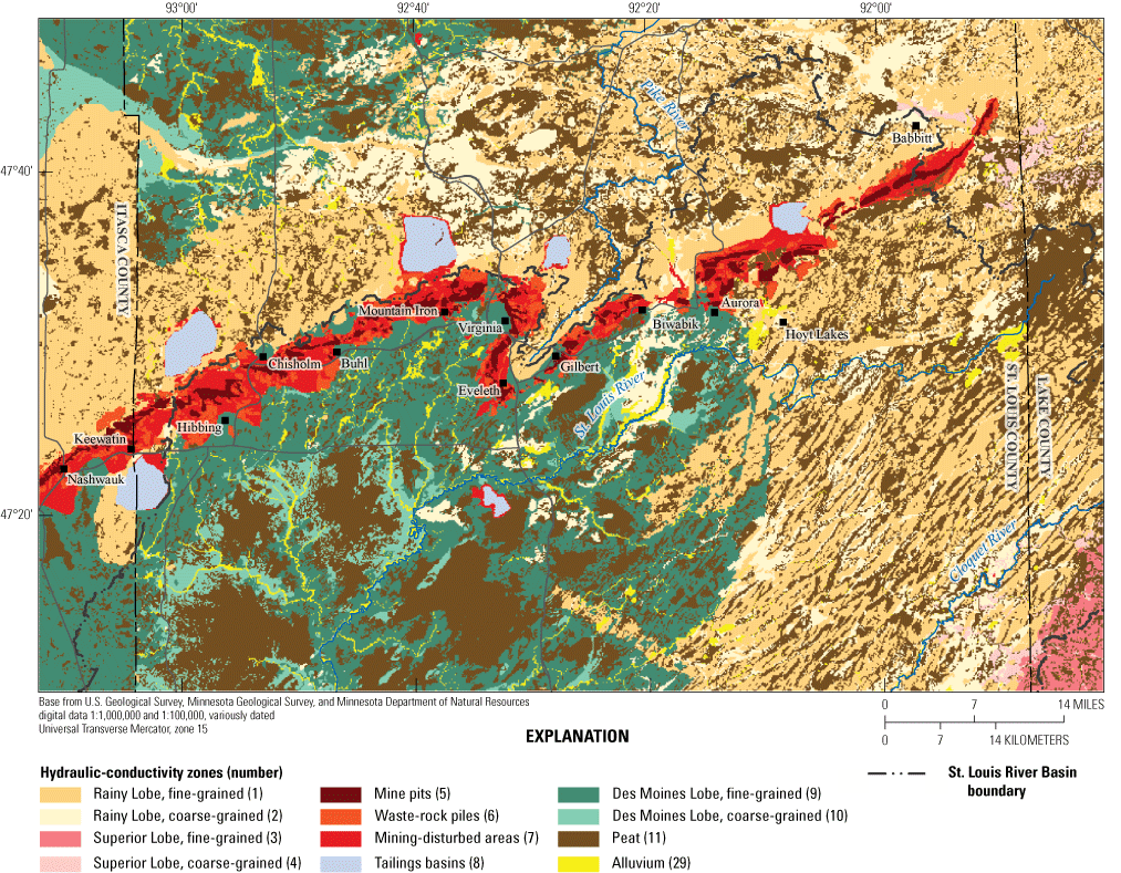
Hydraulic-conductivity zones of surficial sediments, uppermost model layer (1), in the mining model, northeastern Minnesota.
In model layers two through four, layer thickness and glacial materials were stratigraphically modeled in three dimensions using Groundwater Modeling System software (AQUAVEO, 2018) and borehole data from the Minnesota Well Index (T. Wahl, MGS, written commun., 2018; publicly available data at https://www.health.state.mn.us/communities/environment/water/mwi/index.html) (fig. 6). Borehole stratigraphy was generalized into two groups: coarse-grained (sand and gravel) and fine grained (tills and lake clays). Each well had no more than four glacial layers, accommodated by the four glacial layers of the model. The area of Rainy and Superior glacial lobes mapped at the surface were assumed to extend to bedrock throughout the mining-model area. The area of the St. Louis Sublobe was assumed to exist only in layer 1 of the model because it was the last glacial lobe to be deposited in the IRMA (Wright, 1972). Glacial material thickness is greatest (fig. 2) in the south and southwest of the IRMA where bedrock dips away from the Iron Range and St. Louis Sublobe (Des Moines Lobe) deposits overlie the Rainy Lobe deposits (fig. 4). To the north of the Iron Range, glacial material is thin to absent over bedrock (fig. 2).
Model Bedrock Topography and Geology
The elevation of the bedrock surface is derived from a mosaic of preliminary rasters of bedrock topography (in order of precedence) for the southeast (M. Jirsa, MGS, written commun., January 30, 2018) and central (Jirsa, 2016) portions of the MGS Arrowhead study area and the MGS statewide bedrock topography raster (Jirsa and others, 2010). These data were generalized to define the top elevation of model layer 5. In some cells where glacial sediments are thin or absent, the less detailed and interpolated bedrock-surface elevation was higher than the more accurate, measured lidar land-surface elevation. In these cells, the bedrock surface was adjusted to below land surface, and glacial layers were pinched (figs. 3 and 6). Bedrock hydraulic-conductivity assignments reflect our conceptual model that fracturing decreases with depth, such that layer 5 is highly fractured, 6 is moderately fractured, 7 is minorly fractured, and 8 is unfractured. This assumption is based on observations of bedrock at land surface and drill cores made by geologists of the MGS (M. Jirsa, MGS, oral communication, January 30, 2018.).
Bedrock geology from Jirsa and others (2011) was simplified broadly into the four previously described hydrostratigraphic units. The third dimension for the bedrock was generated by simply offsetting to the southeast the contacts of the Biwabik Iron Formation (red areas in figs. 3 and 6) and other bedrock at a dip angle of 15 degrees. The contact between the Duluth Complex and other bedrock is assumed to be vertical. Each of the four bedrock hydrostratigraphic groups (defined in the bedrock geology section) has four hydraulic-conductivity zones with thicknesses shown in table 1 (figs. 3 and 6). Zones of high hydraulic conductivity were added in mine pits to allow for seepage along the edges of the mine pits. The depth to which the mine-pit hydraulic-conductivity zone extended was determined using the minimum lidar elevation in each cell.
Model Boundaries
Groundwater flows into and out of the lateral and top boundaries of the IRMAs; no flow is assumed to flow across the bottom boundary of the model. Flows through the top of layer one include areal recharge, exchanges with streams and lakes, and exchanges with mining features where geologic material has been moved or removed and groundwater flows have thereby changed.
Lateral flows through the boundaries of the mining model were extracted from the regional two-dimensional model of the St. Louis River Basin (Haserodt and others, 2019) and were applied as specified flows to the lateral edge cells of the mining model using the MODFLOW Well (WEL) package. The two-dimensional horizontal model flows were apportioned to the eight model layers based on the initial transmissivity of each layer. The transmissivities of each cell at the model lateral boundary were determined using the pre-calibration hydraulic conductivity estimates for the geologic materials in each cell.
Potential areal recharge through the top of the model was calculated using a Soil-Water Balance (SWB) models described by Haserodt and others (2019). Potential areal recharge is the amount of groundwater recharge plus water that cannot infiltrate to the water table (rejected recharge) either because the infiltration rate is greater than what the aquifer can transmit or because the water table is very near the land surface. The potential areal recharge array was a combination of results from two SWB models. The first is a detailed St. Louis River Basin SWB model (Smith, 2017), which has a 328-ft (100-m) resolution and annual potential-recharge estimates during 1995–2010. The second is a general statewide SWB model (Smith and Westenbroek, 2015), which has 3,281-ft (1,000-m) resolution and annual potential recharge during 1996–2010. Both SWB models were updated to include 2011–15 using the same DAYMET weather data as the original models (Thornton and others, 2014). The results of the St. Louis River Basin SWB detailed model took precedence areally, and the annual SWB potential-recharge during 1996–2015 were averaged to produce the steady-state SWB potential recharge into the mining model (fig. 8). The mining-model potential-recharge array was divided into upland (nonwetland) and wetland areas for the purposes of calibration. These areas were delineated using maps of wetlands from the MGS in St. Louis and Lake Counties (Jirsa, 2016) and from the areas of permanent wetlands (defined in the “Model Surficial Geology” section) in the NWI in Itasca County (MN–DNR, 2018).
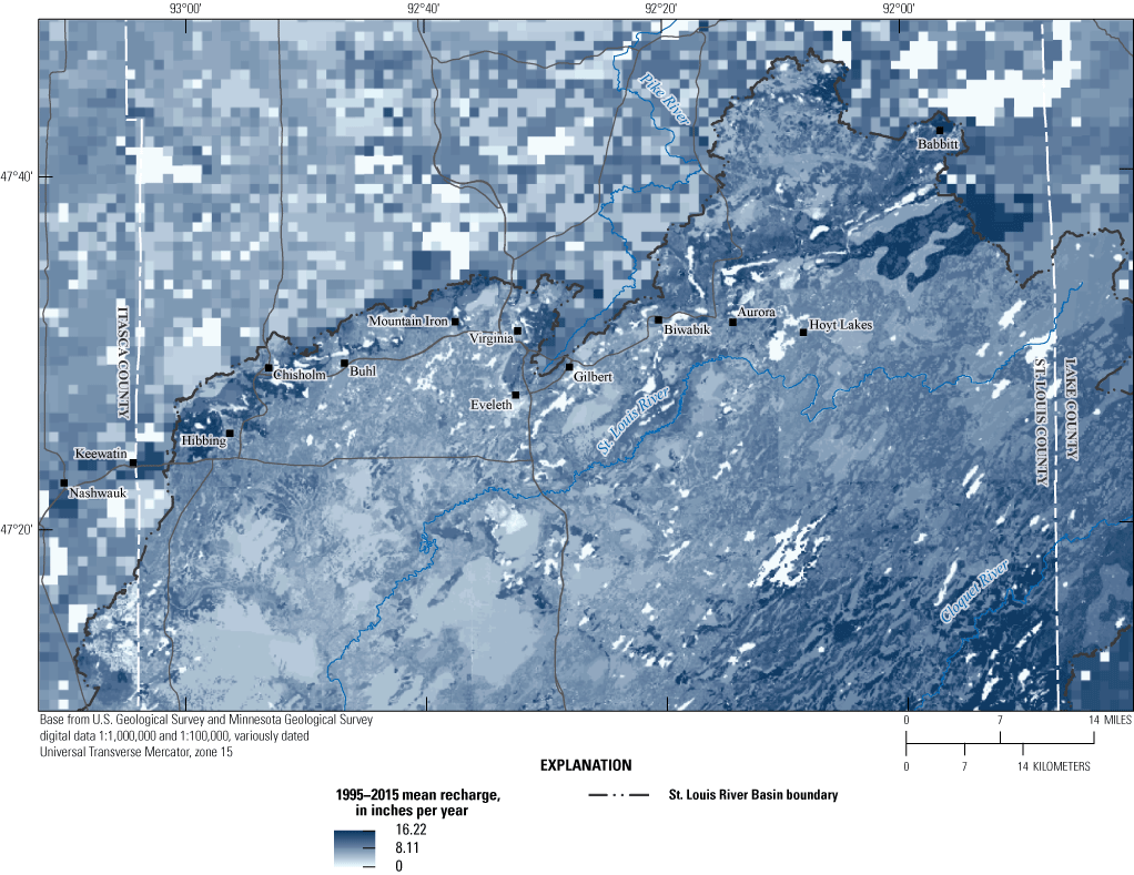
Soil-Water Balance model potential areal recharge to the unsaturated zone in the mining model, northeastern Minnesota.
Hydrologic Stresses
Hydrologic stresses are features that can introduce or remove water from the groundwater-flow model that are not part of the groundwater-flow system itself. Most of these stresses are at the land surface (for example, streams, lakes, and areal recharge), but some, like withdrawal wells, can be within a modeled aquifer itself. Most hydrologic stresses in the model are represented as head-dependent flux boundaries using four MODFLOW packages (SFR2, RIV, DRN, and GHB packages, table 2).
Table 2.
MODFLOW representations of hydrologic features, mining model, northeastern Minnesota.[MODFLOW, U.S. Geological Survey Modular Three-dimensional Finite-Difference Ground-water Flow model; SFR2, MODFLOW Streamflow-Routing 2 package; ft, foot; NAVD 88, North American Vertical Datum of 1988; —, no data; ft2/d, square foot per day; d/ft1/3, day per foot to the one-third power; RIV, MODFLOW River package; ft2, square foot; K/tb, hydraulic conductivity divided by bed thickness; UZF, MODFLOW Unsaturated-Zone Flow package; ET, evapotranspiration; MNW2, MODFLOW Multi-Node Well package 2; ft/d, foot per day; DRN, MODFLOW Drain package, K, hydraulic conductivity; GHB, MODFLOW General-Head Boundary package]
Streams were represented using the Streamflow Routing 2 package (SFR2; Niswonger and Prudic, 2005; fig. 9). SFR2 represents streams as head-dependent flux boundaries and routes stream base flow downstream. SFR2 ignores streamflow contributions from overland flow. The amount of flow between the stream and the water table is determined by the product of the water-table/stream gradient and the streambed conductance. If simulated water-table heads are lower than stream stage, SFR2 calculates the stream loss to groundwater, as long as water exists in the stream channel within the cell. If simulated water-table heads are higher than stream stage, SFR2 calculates the amount of base flow that flows to the stream within the cell. The SFR2 input file was created using the tool sfrmaker (https://github.com/aleaf/SFRmaker, Leaf and others, 2021) with the required stream characteristics (width, depth, flow direction) derived from the National Hydrography Dataset, NHDPlus v2 (McKay and others, 2012). Stream- and lake-surface elevations were determined from the lowest cell in the 1-m lidar digital elevation model (DEM; MN–DNR, 2011) in the model cell area. The thickness of the streambed was assumed to be 1 ft in all reaches. Initial streambed conductance was assumed to be 5 feet squared per day. Streams are routed as fictitious channels through lakes to permit downstream routing. Where stream channels cross lakes, the streambed conductance was set to 1×10⁻⁶ foot per day (ft/d) to prevent the fictitious channels from exchanging water with the lakes. In those cells, groundwater/lake exchange is controlled by lake stresses described later.
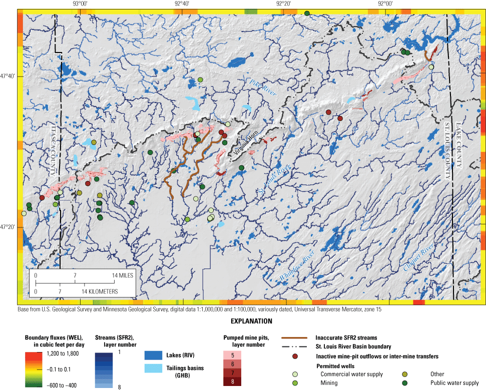
Hydrologic boundaries and stresses in all layers, mining model, northeastern Minnesota. [WEL, well; SFR, streamflow routing; DRN, drain; SFR2, MODFLOW revised Streamflow Routing package; MNW2, multi-node well; RIV, river; GHB, general head boundary]
This procedure produced realistic SFR2 hydrologic stresses throughout the model except in two areas (brown lines in fig. 9): area 1—that part of the Dunka River and its tributaries from 3 mi upstream from where it crosses between mine pits on a narrow land bridge, downstream to Birch Lake and area 2—the first 4 mi (or less) of small headwater streams immediately south and west mine pits in the Virginia Horn. Because the upstream parts of these stream segments are within a model cell that includes a deep mine pit, the elevations of these segments were erroneously set to the bottom of the mine pit instead of the stream surface. All SFR2 hydrologic stresses downstream from these erroneous SFR2 stresses were also set to the same too-low elevation until the stream intersected the land surface at that elevation. This error affected the SFR2 stresses in these areas in two ways. First, the elevation of the SFR2 stress head and bottom elevations are too low, often by 100 or 200 feet. Second, the stream stresses appear in a model layer that is too low, usually layer 6, but sometimes layers 7 and 8. These SFR2 stresses, which represent streams, are covered by 100–200 ft of aquifer and are effectively tunnels within the aquifers in these areas. The erroneously low SFR2 stress heads cause erroneously high gradients to these stream segments, increasing the hydraulic driving force toward these streams. This effect is counteracted, however, because hydraulic conductivity of the aquifer in these lower bedrock layers is orders of magnitude lower than the hydraulic conductivity of the geologic material these stream segments actually are in contact with (unconsolidated glacial sediments or highly fractured bedrock). Therefore, although these erroneous SFR2 stresses may produce locally high head gradients toward the streams, the actual distortion in groundwater flow toward and discharge to these streams likely is very small.
Lakes were represented using the river (RIV) package (fig. 9). The elevation of the bottom of the riverbed (representing lakebed) sediments is set 0.1 ft below the lake surface elevation. This has the effect of limiting the amount of water that lakes can contribute to aquifers, but not limiting the amount of water that aquifers can contribute to lakes. Effectively, the amount of water flowing out of lakes to aquifers is determined by the conductance of the lakebed because the lake/groundwater gradient reaches a maximum when the groundwater level is 0.1 ft lower than the lake level. The lakebed (RIV) conductance is set to 1.6×105 feet squared per day throughout the model. This is equal to a hydraulic conductivity of 1 ft/d and a lakebed thickness of 1 ft because the cell area is 1.6×105 ft2.
Mining Features and Well Withdrawals
Two mining features, tailings basins and mine pits, use hydrologic stresses in addition to hydraulic-conductivity zones to model their effects on groundwater (fig. 9). Tailings basins are modeled using the MODFLOW General Head Boundary package (GHB) stresses (light blue, fig. 9; table 2) and using low hydraulic-conductivity zones in the uppermost model layer. The low hydraulic-conductivity zones account for the low hydraulic conductivity of the fine tailings sediments that coat the bottom of the tailings basins. While the low hydraulic-conductivity zone covered the entire area of each tailings basin, GHB hydraulic stresses (represented by a fixed basin stage [based on lidar elevation data] and a basin-lining conductance) are only in cells of the open-water part of each tailings basin. These GHB stresses represent the fact that mining operations constantly keep these pools full of water, potentially recharging groundwater.
Mine pits are modeled in detail using several techniques. Active mine pits are usually pumped to prevent flooding and allow mining, artificially lowering the water table to the mine-pit bottom (pumped mine pits, table 2). The pumping in active mine pits, which were generally pumped dry during the mining-model period, is represented using the MOFLOW Drain package (DRN; shades of pink to maroon, fig. 9). The elevation of the top of layer 1 is set to the mine-pit bottom, and drain cells allow all water discharging into mine pits to be removed from the model, keeping the mine pits dry. Drain stage is set to the minimum lidar elevation within a mine pit cell, representing the bottom of dry mine pits.
Inactive mine pits have been allowed to naturally fill completely with water or have their water level maintained somewhat lower by pumping or through a constructed or natural surface-water outlet (flooded mine pits, table 2). Inactive, flooded mine pits with no pumping or outlet have the top of model layer 1 set to the pool elevation (mean lidar elevation of the pool area), and model cells representing the water-filled volume of the mine pits are assigned a hydraulic conductivity of 1,121.044 ft/d in layer 1, 1,000 ft/d in layers 2–6, and 16.847 ft/d in layer 7. This choice allows any water entering a flooded mine pit to easily flow to any other cell in the same mine pit. Because depth data are unavailable, mine-pit bottom elevation is assumed to be 101 ft deeper (to the bottom of layer 6) than the pool elevation. No pool water level was imposed on flooded mine pits. Instead, MODFLOW calculated the water level in flooded mine pits based on the groundwater levels adjacent to the mine pits and water flows into, through, and out of the mine pits. The actual, measured pool elevation was used as a guide in calibration.
Inactive mine pits with pumped or surface-water outflows (lowered pools) are modeled with the same general approach used for mine pits with no pumping or surface-water outlets. In mines with lowered pools, mine-pit outflows are controlled by the stage of DRN hydrologic stresses placed throughout the area of the pit and in the appropriate model layer determined from the lidar elevation of the pool. The amount of flow from these DRN stresses are aggregated for each mine pit. These modeled flows are compared to flux targets in model calibration where measured mine outflows were reported in 2011 (A. Guertin, MN–DNR, written commun., 2019; R. Clark, Minnesota Pollution Control Agency, written commun., 2019), the same year that the lidar data used to determine the mine-pit pool elevations were collected.
Estimates of outflows from inactive mine pits during 2011 are available from the MN–DNR and Minnesota Pollution Control Agency (A. Guertin, MN–DNR, written commun., 2019; R. Clark, Minnesota Pollution Control Agency, written commun., 2019) for seven sites that do not discharge into streams with measured flow in the IRMA. Because these inactive mine-pit outflows cannot be used to help calibrate the model, the flows are represented using the MODFLOW Multi-Node Well 2 package (MNW2) (brown dots, fig. 9). Annual 2011 groundwater withdrawals from municipal, commercial, and industrial, nonmine-pit wells that require reporting to the MN–DNR (https://www.dnr.state.mn.us/waters/watermgmt_section/appropriations/wateruse.html, accessed April 2019) were also represented by the MNW2 package in the mining model (green-shaded dots, fig. 9). The MNW2 package was used for these features so that these features could be easily separated from lakes, which were modeled using the WEL package, in model mass-balance results.
All DRN hydrologic stresses (pumped mine pits, flooded mine pits with lowered pools, or mine pits with measured flows) were placed in cells of bedrock layers (5–8) because the mine pits are always constructed in the Biwabik Iron Formation. For each mine pit, DRN hydraulic stresses were assigned to cells in the bedrock layer containing the minimum lidar elevation of that mine pit. Because glacial sediments have been removed from mine pits, the thickness of these upper four layers (1–4) over mine pits is set to 0.25 ft each. Any model layer representing glacial material over a mine pit was given a very high hydraulic conductivity (see description of flooded mine pits, mentioned earlier) to ensure that water discharging to mine pits laterally from those layers can easily flow to DRN hydrologic stresses in the bedrock toward the bottom of the mine pit.
Waste-rock piles and mining-disturbed areas are represented as separate zones of moderately high hydraulic conductivity with no additional hydrologic stresses. These piles sit above the general land surface and consist of large pieces of broken hard bedrock, which justifies the moderately high hydraulic conductivity.
Wetlands
Wetlands are extensive within the IRMA (29 percent, areally), especially in the southeast, and are areas of substantial groundwater/surface-water interactions. Because the model is steady state, only permanent (wet throughout the year) wetlands are simulated. Wetlands are typically simulated in MODFLOW as a hydraulic stress, with a package such as the GHB package (Anderson and others, 2015). Instead, the mining model relies on the UZF package to simulate the flows between groundwater and wetlands using an approach by Feinstein and others (2020). The UZF package is more appropriate to simulate wetlands than the GHB package because the GHB package stresses may over constrain the modeled groundwater heads in the large wetland areas of the IRMA.
The UZF package can limit the amount of potential recharge (from SWB models) reaching the water table (actual recharge) if the unsaturated-zone geologic material is unable to transmit all the specified potential recharge. The difference between actual recharge and the specified potential recharge is called rejected recharge. Where groundwater levels are at land surface, UZF can also permit groundwater to seep to the surface if simulated groundwater heads are above land surface. This is called (areal groundwater) surface seepage. UZF increases surface seepage until groundwater heads decrease to land surface. Where there is groundwater-surface seepage in a steady-state model incorporating UZF, groundwater levels will be very near the surface, all potential recharge will be rejected, and permanent wetlands exist.
The UZF package uses a variable called SURFDEP to control not only where surface seepage occurs, but also where potential recharge is rejected because high groundwater levels prevent infiltration. If the groundwater head in a cell is within half of the SURFDEP distance to the cell top (land surface), all recharge will be rejected, and surface seepage can occur. The SURFDEP distance can be thought of as the average height of land-surface undulation in the wetland areas of the IRMA (Feinstein and others, 2020). In the IRMA, the average land-surface undulation within areas mapped as wetlands is about 1 ft in height (based on lidar data), and this measurement was used as the SURFDEP value throughout the model. The UZF package was not active in cells containing lakes or mine pits (fig. 10). For the purposes of defining wetlands in model output, any area with simulated areal groundwater-surface seepage to the land surface (and, by definition, any area where the water tables is within plus or minus 0.5 ft of the land surface) is considered a simulated permanent wetland. Areas of simulated permanent wetlands were compared to areas of mapped permanent wetlands derived from M. Jirsa (MGS, oral commun., January 30, 2018) and MN–DNR (2018) (see peat, in the “Model Surficial Geology” section, for details). Areas where simulated permanent wetland (presence or absence) disagrees with areas of mapped permanent wetland are a measure of the degree to which the model accurately simulates the IRMA wetland hydrology.
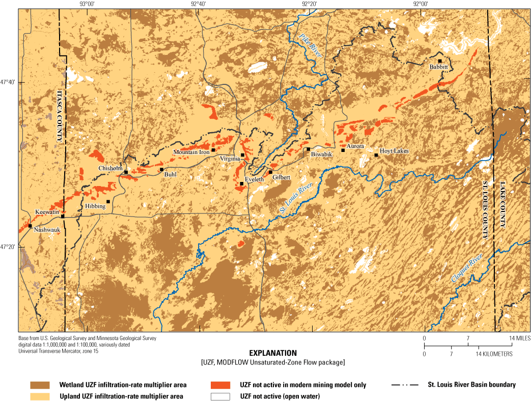
Unsaturated-zone simulation and potential-recharge multiplier areas, mining model, northeastern Minnesota.
The mining model does not use the overland-flow routing function of the UZF package, so rejected recharge and surface seepage from UZF appear as separate lines in the model water balance. The amount of rejected recharge and surface seepage that makes its way to become streamflow must be added to base flow outside of MODFLOW in postprocessing. A water-cycle study of a wetland-rich area of northwestern Minnesota found that approximately 86–87 percent of groundwater discharge left the study area as ET (Cowdery and others, 2019). Much of the groundwater discharges to closed-basin wetlands, rather than flowing streams, before evaporating or transpiring. Although the wetland-rich IRMA is somewhat wetter (13 percent wetter than average annual precipitation of northwestern Minnesota during 2003–15) and cooler (Smith and Westenbroek, 2015) than northwestern Minnesota, the importance of ET fluxes in the IRMA is also likely to be substantial. Rejected recharge likely occurs mostly in permanent wetland areas where groundwater levels are persistently at land surface. Although these wetlands are extensively ditched for agriculture, the ditches usually contain substantial vegetation, especially in the summer. This vegetations plugs up ditches, keeping water levels higher and making them less able to drain nearby wetlands. This leaves water on the landscape where it can evaporate. Therefore, 80 percent of the rejected recharge was assumed to leave the Basin through ET. The remaining 20 percent was added to the appropriate stream base flow by a postprocessing utility as part of the calibration process.
In contrast to rejected recharge, most areal surface seepage likely occurs low in the landscape, near and beneath streams as springs, where upward vertical hydraulic gradients are highest. Little of this seepage would be lost to ET because the seepage discharges close to streams and quickly flows to them. Although stream water also evaporates, stream surface area is relatively small compared to the flux of water in the stream. Therefore, we assumed that only 20 percent of surface seepage left the model through ET, and the remaining 80 percent was added to the appropriate stream base flow by the postprocessing utility as part of the calibration process.
Calibration of the Mining Model
The mining model was calibrated with parameter-estimation software (PEST; Doherty, 2010, 2014) using the guidelines of Doherty and Hunt (2010). PEST adjusts model variables, called parameters, within modeler-specified bounds to minimize the difference between measured (observed) and model-calculated groundwater heads, base flows, mine-pit outflows, and wetland areas. Observations are weighted according to the importance and accuracy of the measurements so that better observations have a bigger effect on the calibration of the model. The sum of the weighted difference between the model-calculated result and the measured observation is called the objective function. PEST adjusts parameters to minimize the objective function and calibrate the model. PEST was used in a stepwise fashion to reduce computational time and to control how the objective function was minimized (described later).
Observations
PEST calibrated the mining model to measured groundwater levels, stream base flow, mine-pit dewatering flows, and the degree to which the model correctly simulated wetland and nonwetland areas (discussed later). Of the 2,766 measurements forming the water level calibration dataset (fig. 11), 2,629 groundwater levels came from the Minnesota Well Index (T. Wahl, MGS, written commun., 2018, publicly available data at https://www.health.state.mn.us/communities/environment/water/mwi/index.html), which is maintained by the Minnesota Department of Health; 55 were supplied by the MN–DNR (2016); and 8 were supplied by the Minnesota Pollution Control Agency (A. Streitz, written commun., 2018). All calibration water levels are available in the model archive (Cowdery and others, 2023). The remaining 74 groundwater levels were from mine pits and mine-pit lakes determined from 2011 lidar elevation data. Most groundwater levels were single measurements (table 3) collected during drilling or development of wells for domestic, municipal water supply, and mining exploration uses. Average water levels were calculated at wells with more than one water level. Only levels from wells where the aquifer was known were included. Levels used for calibration were measured during 1900 to 2017, with 97 percent of those measurements being collected after 1970. Most measurements are from the 1990s and 2000s (25 percent and 30 percent, respectively). Fifty-seven percent of the water level observations were measured during the steady-state modeling period of 1995–2015, but during 2011, the year corresponding to lidar measurements used in determining lake and mine-pit water levels, only 3 percent (83 water levels) were available.
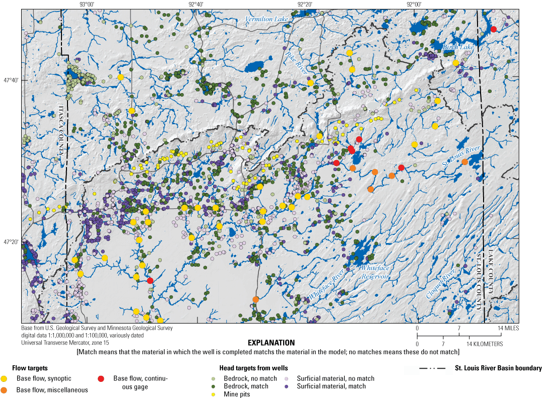
Location of water levels and stream flows used in calibration in the mining model, northeastern Minnesota.
Table 3.
Water levels at wells in the Minnesota Well Index used to calibrate the mining model, northeastern Minnesota.Base flow in streams (fig. 11) measured by the USGS and MN–DNR falls into three groups when used for calibration: base flow calculated at continuous-flow streamgages (7 sites), miscellaneous single streamflow measurements (6 sites), and streamflow from a group of sites (34 sites) at which one-time, concurrent synoptic flow was measured (table 4). All flow measurements were modified to model units (cubic feet per day [ft3/d]) and to better represent the steady-state period that the calibrated mining model simulates. A base flow estimate was calculated from continuous streamflow records at seven streamgages by hydrograph separation using the Institute of Hydrology Base Flow Index method (Institute of Hydrology, 1980; Wahl and Wahl, 1988). During 2012–15, four of these sites had complete daily average flow records. Three other sites had substantial daily flow records, but these records were incomplete during 2012–15. The incomplete sections of the records were estimated by calculating an average flow factor for the streamgage with missing records during periods of overlapping flow record with the USGS streamgage (USGS site 04015438) in the St. Louis River headwaters at Skibo, Minnesota (average daily flow at the Skibo streamgage during the period of overlapping record divided by the average daily flow at the Skibo streamgage during 2012–15). This average flow factor, multiplied by the average streamflow at the Skibo streamgage during missing streamflow periods, produced a complete average daily streamflow estimate for the streamgage with missing flow record for the 2012–15 period. Average daily base flow discharge, which was assumed to be groundwater discharge, was calculated at these seven sites during 2012–15.
Table 4.
Observations and objective-function weight used to calibrate the mining model, northeastern Minnesota.[>, greater than; <, less than; —, not applicable]
Six miscellaneous, single flow measurements stored in the USGS National Water Information System database (USGS, 2022) and collected during 2012–15 were also used as flow observations in calibration. These measurements were corrected to produce 2012–15 representative flows using a factor of the flow at the Skibo streamgage on the measurement day divided by the average base flow at the Skibo streamgage during 2012–15. One set of synoptic streamflow measurements was collected for this study at 34 locations on August 15–17, 2018. The 34 synoptic measurements were also adjusted to produce 2012–15 representative flows with the same method used to adjust the miscellaneous flow measurements.
The flows of rejected recharge and surface seepage calculated by the UZF package are important components of the water budget in the IRMA, and some part of these flows likely contributes to base flow measured and used as flow calibration targets in the mining model. The rejected recharge and surface seepage that do not find their way to streams are eventually lost to ET. To accurately calibrate the model, the flows not lost to ET were added to model-produced stream base flows using a post-MODFLOW processing utility program because they are not routed within the implementation of the UZF package used. As noted previously, 20 percent of the rejected recharge was assumed to not leave the Basin through ET and was added to the appropriate stream base flow. In contrast, 80 percent of surface seepage was assumed to not leave the Basin through ET and was added to the appropriate stream base flow
Reported dewatering flow at 16 mine pits was also used as calibration flow targets. The aggregated outflow of DRN hydrologic stresses for each mine pit, which is used to maintain mine-pit water levels in the model, was compared to the average reported mine-pit dewatering flow. Aggregated dewatering flows were routed (as part of the postprocessing) to the appropriate streamgages to augment simulated stream base flows. Two mine pits on the western end of the IRMA were within the Mississippi River drainage area where streamflows were not measured. The discharge from these mine pits was not routed.
Total area of mapped permanent wetland in the IRMA was used as an observation (brown areas, fig. 10) and compared to total permanent wetland area produced by the model (area of groundwater-surface seepage. See definition of model-produced wetland area in “Wetland” section presented previously). The difference in these areas multiplied by a weighting factor of 0.004 (table 4) was added to the objective function, which was minimized during PEST calibration. Two types of wetland-area errors are possible. False-negative wetland areas are those where mapped wetlands exist, but the model does not produce surface seepage. False-positive wetland areas are those where there are no mapped wetlands, but the model produces surface seepage.
Weights
Weights were applied to the water levels to control their importance in parameter estimation. Calibration water levels were placed in the model layer corresponding to the depth of the well open interval. For wells where the geologic material of the open interval did not match that of the containing model layer, observation locations were moved vertically by as much as 80 ft to an adjacent cell that had matching geologic material. Observations that were moved received lower weight in calibration; water levels from wells with an open interval in geologic material that matched that of the corresponding model cell have more weight (number of water levels matching or not matching for each type of material is shown in table 5). Water levels from wells that are within three model cells of a boundary condition (including hydrologic stresses) also have less weight because specified fluxes at the lateral boundaries can produce modeled groundwater heads that are substantially different from measured heads. The weights used for calibration water levels are shown in table 4.
Table 5.
Calibration water levels and group codes for the mining model, northeastern Minnesota.[WL, water-level; PEST K, horizontal hydraulic-conductivity zone for Parameter Estimation software; HS, hydrostratigraphic; PPs, number of pilot points; —, no zone; FG, fine-grained; CG, coarse-grained; SLSL, St. Louis Sublobe of the Des Moines Lobe; Fm., formation; Gran./cryst., granite/crystalline]
Number of water levels from wells with open-interval material that match or do not match (no match) the model material.
Zone code for calibration water levels. The first code number contains wells where the open-interval material matches the model material. The second code number contains wells where these materials do not match.
The weights applied to base flow observations favored values calculated from continuous hydrographs and those with higher flows (table 4). Weights were calculated by taking the appropriate weight dividend from table 4 and dividing it by the base flow to produce the weight used for that base flow. Average base flows calculated from continuous hydrographs have high weight dividends that produce relatively high weights because they better represent the average flow conditions that a steady-state model produces. Single base flow measurements have relatively low weight dividends that produce relatively low weights because these measurements are idiosyncratic of the flow conditions at the time of measurements and may not represent the long-term average conditions produced by a steady-state model. High base flow had higher weight dividends because higher flows were measured at locations that have a larger drainage area, thus integrating a larger part of the model. The choice of these weights ensures that the overall groundwater flows through the model have more effect on parameter values than do flows from a small area of the model.
Mine-pit discharge measurements were all given a relatively low weight of 20 because they have a large uncertainty and are all about the same magnitude. The weight for wetland false-positive area and false-negative area observations were 0.004, which is small, because the method used to determine the wetland area in a steady-state condition in the IRMA is uncertain, as described previously. Further, the method used to determine what areas of the steady-state model are wetlands also contains many assumptions and uncertainties.
Parameters
Model hydraulic conductivity was initially calibrated using zones (layers 1, 7, and 8) and pilot points (layers 2–6; Doherty, 2003). Pilot points is a parameterization method where values of the parameter are estimated at modeler-specified locations in the model. The model hydraulic-conductivity arrays were interpolated from the hydraulic conductivity at pilot-points using modeler-specified estimation choices. This approach offers a compromise between the computationally burdensome option of specifying a parameter in every model cell and the rigid representation of specifying a parameter in a small number of constant hydraulic-conductivity zones (Hunt and others, 2007; Anderson and others, 2015). Singular-value decomposition (Kalman, 1996; Aster and others, 2013) was used to ensure stability in the parameter-estimation process using settings suggested by Doherty and Hunt (2010). Tikhonov regularization (Tikhonov, 1963a; Tikhonov, 1963b; Doherty, 2003; Doherty, 2010) was used during parameter estimation to prevent overfitting (that is, unrealistic parameter values) following the approach of Doherty and Hunt (2010). See Doherty and Hunt (2010), Anderson and others (2015), and Leaf and others (2015) for a detailed description of the application of these methods.
The PEST calibration adjusted 306 parameters: 21 hydraulic-conductivity zones, 252 pilot points in 12 hydraulic-conductivity zones, 29 vertical hydraulic conductivity anisotropy zones, recharge multipliers in 2 zones, and streambed and drain conductance (tables 6 and 7). Pilot points were not used in layer 1 because the available detailed surficial geology mapping was able to provide appropriately heterogeneous hydraulic-conductivity distributions using zones of mapped sediment texture. The glacial geology detail produced for layers 2–4 was much lower than in layer 1 because it was interpolated from a few hundred well logs that had the range of sediment types aggregated into six material groups. Two of these materials (St. Louis Sublobe fine-grained and course-grained sediments) do not appear in layers 2–4. The remaining four glacial materials were treated as single material zones regardless of layer, and their hydraulic conductivity was calibrated using pilot points within those zones. The four bedrock materials in layers 5–8 were given separate hydraulic-conductivity zones in each layer to account for decreased fracturing with depth. Pilot points were placed within the zones in layers 5 and 6 (the uppermost two bedrock layers) because there were enough groundwater head measurements in these layers to inform hydraulic-conductivity variability. Pilot points were not placed in layers 7 and 8, because so few groundwater head measurements were available to constrain pilot point parameters. Piecewise-constant hydraulic-conductivity zones represented the four bedrock materials in layers 7 and 8.
Table 6.
Horizontal hydraulic conductivity of the mining model, northeastern, Minnesota.[Gray shading of cells with “NPP” indicates those zones do not have pilot points and no statistics should be expected. Pink highlight (also marked with a *) is the pilot-point value at the end of its allowed range. Green highlight (also marked with a †) indicates each of layers 2–4 had its own calibrated value based on one pilot point. K, horizontal hydraulic conductivity, in feet per day; PEST, parameter-estimation software; —, not available; NPP, zone had no pilot points; FG, fine-grained; CG, coarse-grained; SLSL, St. Louis Sublobe of the Des Moines Lobe; Fm., formation; Gran./cryst., granite/crystalline]
Horizontal hydraulic-conductivity ranges based on those literature values summarized by Haserodt and others (2019).
Range of generic sand and gravel from northeastern Minnesota; used where horizontal hydraulic conductivity of coarse-grained material from specific glacial lobes was not available.
Table 7.
Automated calibration parameters of the mining model, northeastern Minnesota.[No., number; Kxy, horizontal hydraulic conductivity, PAR, potential areal recharge; —, unitless; ft/d, foot per day]
Detailed in table 6.
The initial hydraulic conductivity for each zone was set within ranges reported from the literature to maintain an appropriate relative ranking of hydraulic conductivity of aquifer materials to one another (table 6). The hydraulic conductivity of Des Moines glacial fine-grained sediments is less than that of the Rainy Lobe, which is less than that of the Superior Lobe, based on the general texture of those tills (Wright, 1972; Johnson and others, 2016). Relations in the variability of hydraulic conductivity in bedrock were incorporated into the model by differing ranges in parameter constraints (table 5). The order of decreasing bedrock hydraulic conductivity is the Biwabik Iron Formation (which also is more highly variable), the Duluth Complex, the Virginia formation, and crystalline bedrock (Barr Engineering Company, 2014). Most upper and lower bounds for pilot-point hydraulic-conductivity parameters spanned two orders of magnitude for each zone, where the initial value was at or near the mean of its range. Zones were given wider bounds to reflect the range of reported literature values and expected upscaling artifacts that may result from using literature values in a groundwater-flow model (table 6). Hydraulic conductivity was initially free to vary in each unit independently during parameter estimation. Optimum hydraulic conductivities were evaluated for reasonableness at the end of the parameter estimation. Vertical anisotropy for each initial hydraulic-conductivity zone was calibrated as a separate parameter (table 7) regardless of whether that zone had pilot points. Using an anisotropy parameter with a lower bound of 1.0 ensured that optimal parameters always had the expected relative relation of horizontal hydraulic-conductivity values being equal or greater to the vertical hydraulic-conductivity value.
The potential areal recharge array was divided into two areas, each with a calibration multiplier parameter: “wetland” recharge areas of low slope and “upland” recharge areas of higher slope (table 7, fig. 10). For the purposes of calibration, wetland areas are those defined as peat accumulating permanent wetlands (see “Wetland” section). All other areas are considered uplands. The two wetland recharge area multipliers retain the relative potential-recharge distribution produced by the SWB model across the IRMA but allow PEST to calibrate the mining model to more closely simulate the correct total flux through the aquifers in the IRMA. The multiplier for upland areas was allowed to vary over a wider range during calibration because the uplands are more variable geologically, hydrologically, and biologically than are the wetland areas.
Mining-Model Results
The water table in the mining model (fig. 12) generally follows the surface topography, with elevations over 1,800 ft along the Iron Range and in the topographically high area along Lake Superior (Superior highlands) to the southeast of the Toimi Drumlin Field (fig. 1). The lowest groundwater elevations are in the downstream parts of the major rivers: the St. Louis in the southwest, the Pike in the north, and the Little Fork (see fig. 1 for location) in the northwest. Within the St. Louis River Basin, groundwater-flow direction is like that of streams: from the Iron Range and Superior uplands toward the St. Louis River and out of the IRMA in the southwest (fig. 12). Groundwater gradients dip steeply south from the Iron Range, and less steeply to the north. These features appear on the cross section A–A′ (fig. 13; trace on fig. 1), which cuts west-east through the center of the IRMA, near the city of Virginia. On the east and west flanks of the cross section, the water table generally follows the topography close to the land surface. Near the topographically high areas of the Iron Range, the water table is deeper in part because of mine dewatering, and its gradient is steeper because of the high topography. Shallow groundwater discharges to surface waters, the Embarrass River, and the headwaters of the St. Louis River in the cross section. Deeper, regional scale groundwater-flow discharges to areas of low hydraulic head: the Embarrass River and dewatered mine pits in the cross section. The McKinley mine pit, for example, has the lowest model-layer-one hydraulic head in the cross section and likely captures some groundwater that otherwise would have discharged to the Embarrass River. Note that a lower hydraulic head in the cross section is at depth between the city of Virginia and the Missabe Mountain mine pit, indicating that all flow is downward in that area. The downward flow likely is the result of the erroneous SFR2 stresses noted in the “Hydrologic Stresses” section. The downward flow may also be caused by some flow that contains a component that is perpendicular to the plane of the cross section toward some lower discharge area. This lower discharge area may be the upper reaches of tributaries of the St. Louis or Pike Rivers or some other pumped mine pit.
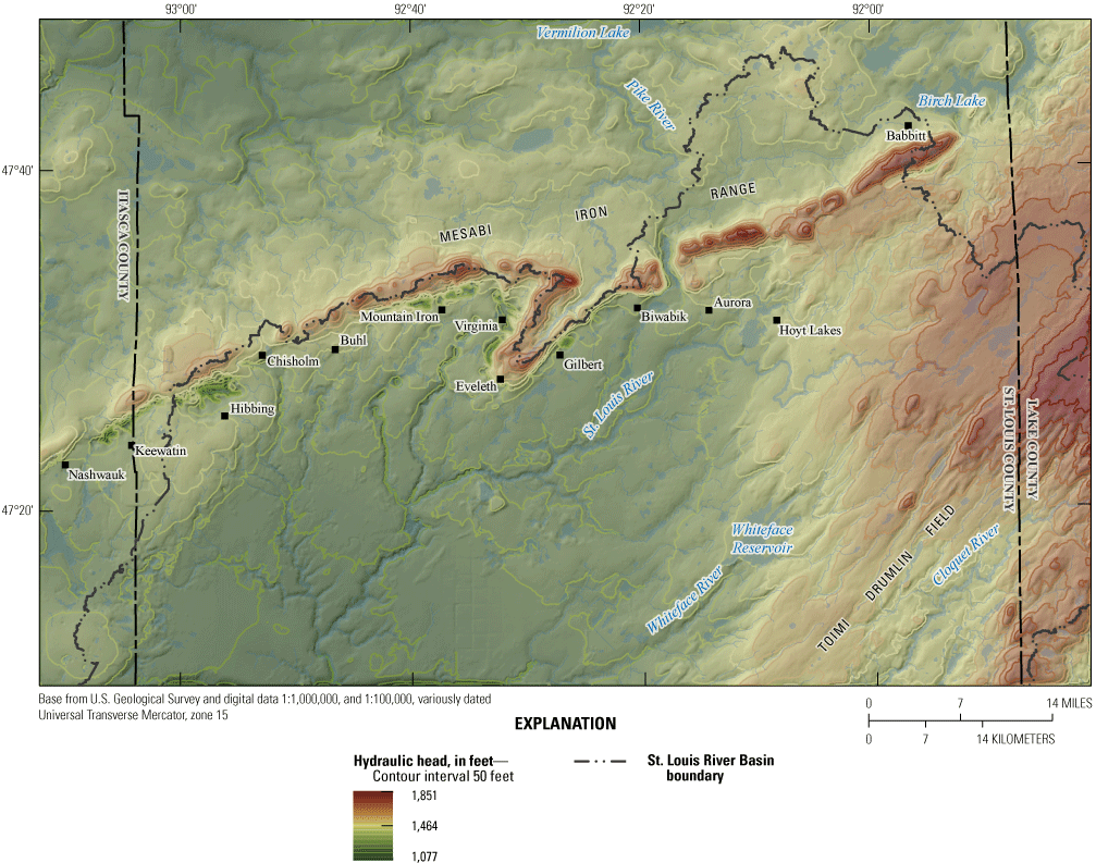
Simulated water-table elevation in the mining model, northeastern Minnesota.
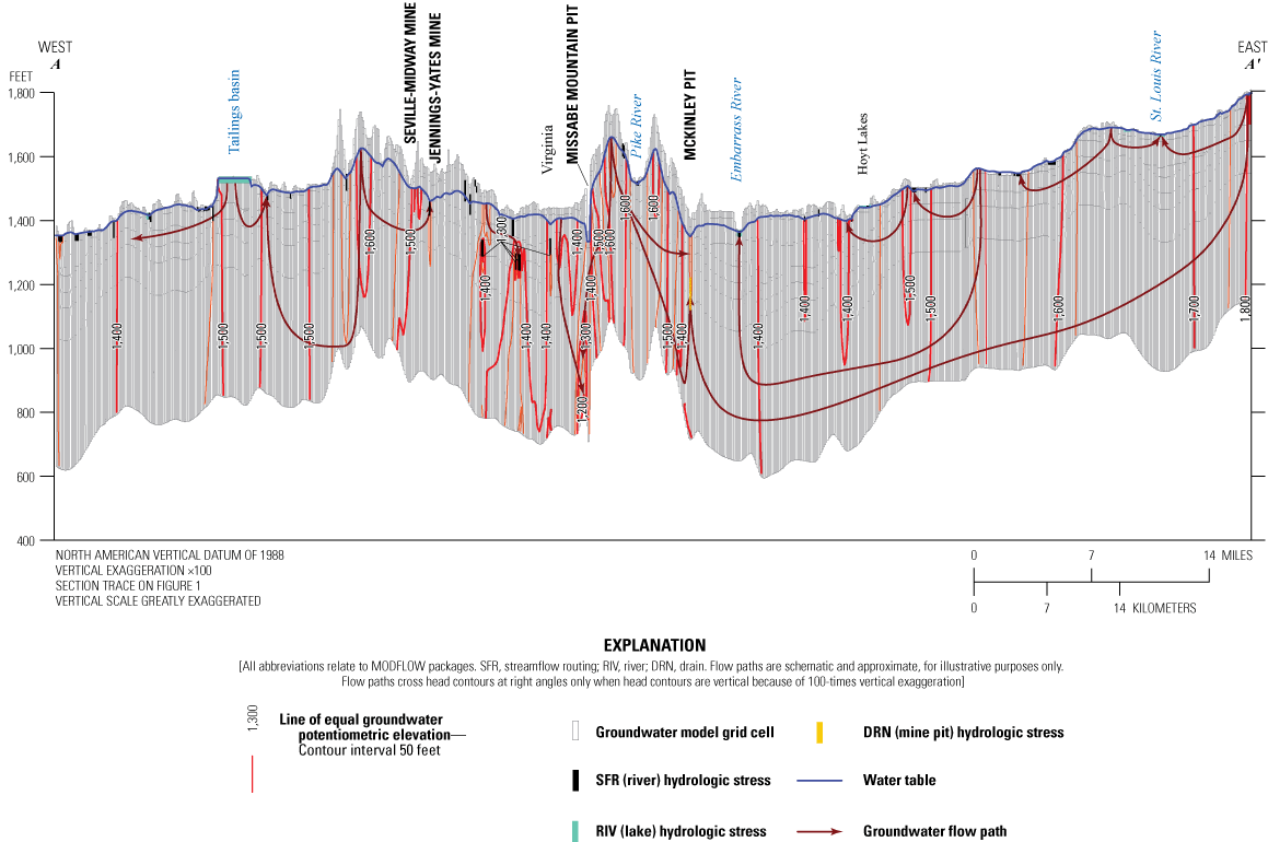
Water-table elevation along the trace shown in figure 6 in the mining model, northeastern Minnesota.
Groundwater discharges to streams (providing stream base flow) throughout most of the IRMA (green reaches in fig. 14). Stream reaches that lose water to aquifers are concentrated near the model boundary. Recall that the model is bounded laterally by WEL package hydrologic stresses that represent groundwater flow into or out of the lateral boundaries (fig. 9). These flows are approximate because they come from a Basin-wide regional two-dimensional groundwater-flow model (Haserodt and others, 2019). These lateral flows are apportioned in the third dimension of the mining model based on the uncalibrated transmissivity of each cell in the vertical stack. Because this apportionment is approximate, some (outward) boundary flow stresses may be too high. Where outward flow stresses occur in cells containing SFR2 stream reaches, flow from streams may be induced where such flows may not actually exist. These unrealistic flows are far from the main mining features that are the focus of this study, however, so they do not affect conclusions drawn from model results. This artificial situation likely occurs at many of the losing stream reaches near the lateral boundary. Apart from the edges of the grid, short losing reaches occur throughout the IRMA, but are nowhere extensive. A broad area of slightly gaining stream reaches (lightest green circles, fig. 14) in the southwestern part of the IRMA coincides with an area of highly ditched wetlands. Model results indicate that this large area is in intimate connection with the groundwater, but that discharge is small (less than 100 ft3/d) there. This may mean that ditches are not particularly effective at draining the wetlands, perhaps being clogged with vegetation most of the time.
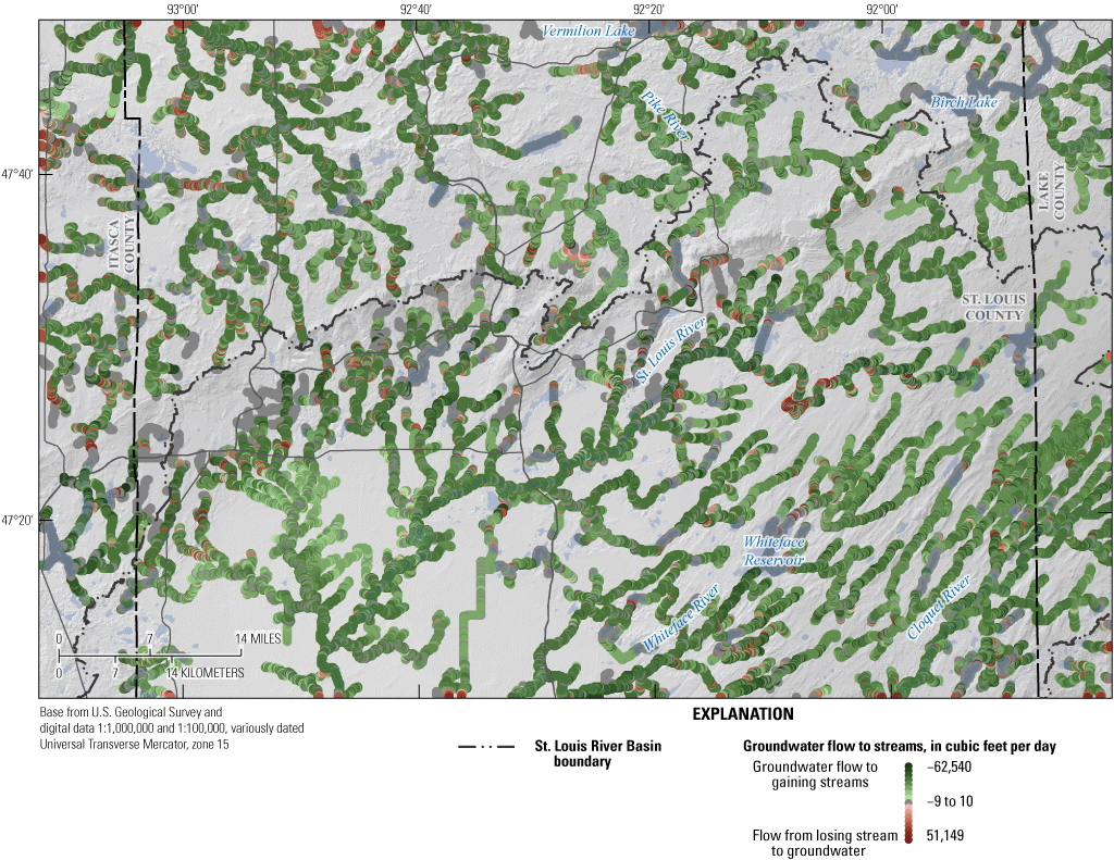
Base flow to streams in the mining model, northeastern Minnesota.
Water Balance
Total groundwater flow through the mining model is nearly 171 million ft3/d. In a steady-state groundwater model, inflows should balance outflows. In this model, the balance is 0.012 percent. The components of the mining-model water balance (table 8) that have the largest flows are areal recharge (in, 78 percent), areal groundwater seepage to the surface (surface seepage out, 45 percent), seepage to streams (out, 43 percent), and stream seepage to groundwater (in, 12 percent). These four flows comprise 90 percent of the model inflows and 88 percent of the model outflows. Flows in other components (for example, inflows and outflows from the model perimeter, lakes, and mine pits) are each less than 5 percent of the total groundwater flow. Simulated model surface seepage occurs throughout the IRMA but is concentrated in the lowlands. Surface seepage rates in areas of extensive wetlands were small (less than 0.01 ft/d per cell), while surface seepage rates occurring near streams were larger.
Table 8.
Water balance, mining model, northeastern Minnesota.[— indicates flows that are not possible. Negative flows mean flow out of model cells. MODFLOW, U.S. Geological Survey Modular Three-Dimensional Finite-Difference Ground-Water Flow model; UZF, MODFLOW Unsaturated-Zone Flow package; %, percent; SFR, MODFLOW Streamflow Routing package; RIV, MODFLOW River package; WEL, MODFLOW Well package; DRN, MODFLOW Drain package; GHB, MODFLOW General Head Boundary package; MNW2, MODFLOW Multi-Node Well package]
Total groundwater flow out to all mining features and pumping wells (man-made features) is 4.1 percent of all groundwater flow. This is partly counterbalanced by groundwater recharge (flow in) from tailings basins of 2.7 percent, leaving net groundwater flow out to man-made features at 1.4 percent. Most of this outflow is mine-pit (dewatering) pumping (2.7 percent), other (nondewatering) mine pumping (0.6 percent), and groundwater discharge to tailings basins (0.4 percent). Coincidentally, the amount of groundwater leaving through mine pits is equal to the amount of groundwater entering from tailings basins (table 8), although some groundwater also flows out to tailings basins as seepage (0.4 percent). The model was only able to produce 55 percent of the specified amount of municipal and industrial groundwater withdrawals without model cells becoming dry. Similarly, only 68 percent of the lateral-boundary flows out of the model could be produced. Together, these unproducible flows are 2.1 percent of total groundwater flow through the model.
Groundwater flow decreases with depth in the model (tables 9–11). More than 80 percent of groundwater flow in the IRMA model occurs in the upper four model layers of surficial and glacial materials; flow between layers (downward, upward, or net flows) decreases by between one-half and one order of magnitude per model layer downward. This pattern reflects the fact that most of the hydrologic stresses (water sources and sinks) and aquifer transmissivity in the model occur in the uppermost layers (recharge, streams, and lakes for example, typically occur in the uppermost four layers). The distribution of this flow in the unconsolidated layers (1–4) likely is not evenly distributed spatially, however. In areas like the northwestern and northeastern part of the IRMA, where these layers are thin (white areas, fig. 2), considerably more groundwater may be flowing in the upper bedrock layers than in other parts of the IRMA. In the bedrock layers (5–8), mine-pit drainage and well pumping create hydraulic gradients that likely result in higher flows than would otherwise occur in the absence of such hydrologic stresses.
Table 9.
Hydrologic-stress flows by layer, mining model, northeastern Minnesota.[%, percentage of total model inflow; BR, bedrock; —, no data]
Table 10.
Water flow between layers, mining model, northeastern Minnesota.[%, percentage of total model inflow; BR, bedrock]
Head Calibration Results
Calibration of the mining model produced a good fit for heads (coefficient of determination, R2=0.93; fig. 15). The mean head residual (measured minus simulated) for all heads was −1.89 ft, indicating that modeled heads are biased slightly low. The mean absolute error residual for all heads was 11.03 ft, with a standard deviation of 14.68 ft. (root mean squared error:18.36 ft.). The mean absolute error of heads measured in 6 of 74 wells in mines and mine pits was more than twice as high as those from other head groups, reflecting the inability of the model’s discretization to capture all hydrologic variability and heterogeneity near mining activities.
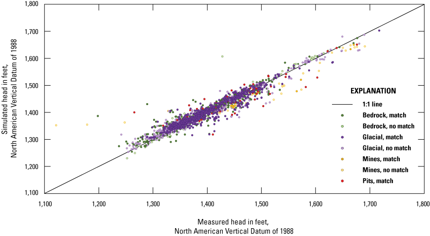
Measured and simulated groundwater-level differences by aquifer in the mining model, northeastern Minnesota.
The difference between measured and simulated heads (modeled head errors) average near zero (−1.89 ft), indicating that the model produces heads that are not substantially biased. Most of large head errors cluster near the mining features of the Iron Range, however, and these errors tend to be positive, indicating that the calibrated model tends to produce heads in this area that are too low. The sign and magnitude of the head errors within each of the seven head groups shown in figures 15 and 16 also appear random, indicating that the calibrated heads are not biased among these groups. Some simulated heads differed substantially (28 heads, 1 percent, greater than 71 ft, absolute value) from the measured heads, however, but are not in any particular group.
Several features of the calibration heads are responsible for the disagreement between measured and modeled heads. The measured heads used to calibrate the model were collected over the last 120 years during times that do not represent a steady state, especially during droughts and wet periods. Further, many of the heads were collected by drillers and reported as water levels below land surface even though measurements are often made from a location higher than land surface. The location of some wells and, therefore, the land-surface elevation derived from DEMs is poorly known, which can affect the elevation of water levels. Because the discretization of the model grid and the geology it contains are crude approximations at the scale of a well, the model geologic material of a cell containing the open intervals of some wells is not the same material as that on the stratigraphic record of the well in the real world. If a model well is finished in a clayey till but the real well is finished in a buried sand, a substantial difference between modeled and measured water level can be expected. Finally, the steady state produced by the model cannot exist in the natural world, so modeled steady-state heads will never perfectly match measured heads.
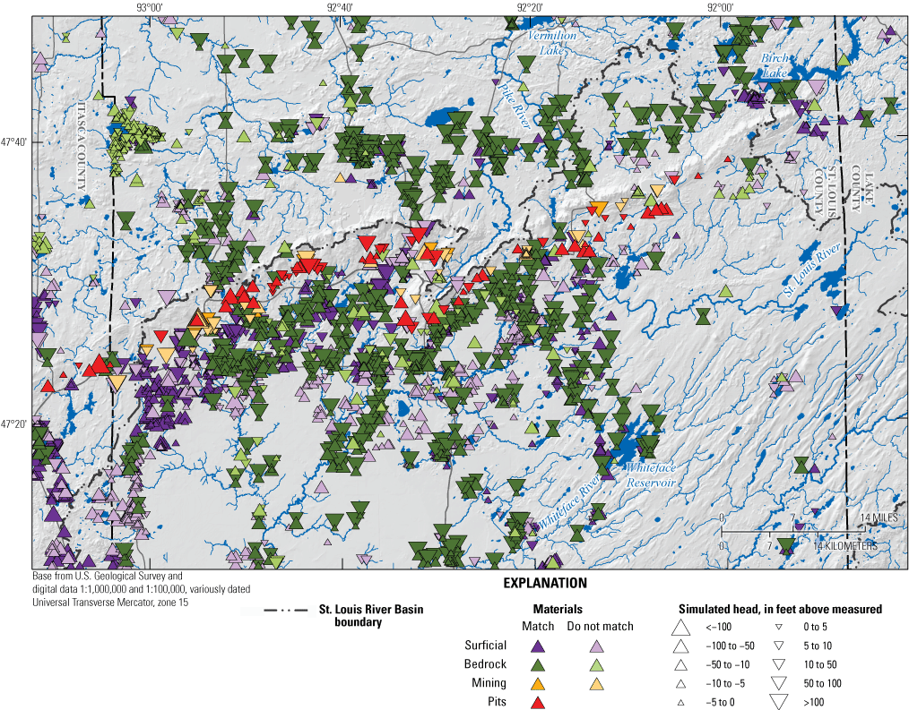
Measured minus simulated groundwater level differences, by aquifer in the mining model, northeastern Minnesota.
Although the model generally simulated water levels well, water levels from mine pits and water levels near other mining features have larger residuals than water levels in areas with geologic materials. Part of the error in simulated mine-pit water levels likely is because of the heterogeneous hydraulic conductivity of the Biwabik Iron Formation and the overlying coarse-grained glacial deposits that supply the mine pits with water. The density of measured water levels and, therefore, pilot points used in the model are inadequate to capture all the geologic variability in the IRMA. Further, mine-pit water levels were determined from the 2011 lidar DEM. This year was drier than average and did not represent the long-term steady-state heads that the model produces. The large head residuals near nonmine-pit mining features likely come from their proximity to mine pits, which induce large head gradients that change constantly as mine pits are developed and dewatered. Finally, the locations of bedrock wells (and their water levels) are likely skewed toward parts of bedrock that locally have higher hydraulic conductivity. Well drillers likely select these locations for wells because they produce more water. Because the model calibration is dependent on measured water levels from these higher hydraulic-conductivity locations in the bedrock, the final bedrock hydraulic conductivities in the model likely are closer to the real average bedrock hydraulic conductivity in the IRMA, not the higher hydraulic-conductivity locations of wells. This would result in higher head errors near productive wells.
Head errors in bedrock are also generally very large (more than 100 ft) near mines, and nearly all of the residuals greater than 30 ft occur along the Iron Range (fig.16). A disproportionate number of these large residuals occur in the Biwabik Iron Formation for the reasons outlined previously: the formation’s hydraulic conductivity is heterogeneous, and many water levels come from mine pits, which are themselves heterogeneous. While 6.5 percent of heads errors were greater than 30 ft, 57 percent of these are in the Biwabik Iron Formation. Other bedrock zones had fewer than 5 percent of these large head errors.
Flow Calibration Results
Simulated base flow at streamgages also match measured streamflow well (R2=0.97 or greater of all but miscellaneous base-flow measurements; figs. 17 and 18). The model’s ability to reproduce flow is affected by several factors. Average flow at continuous streamgages is based on long periods of many measurements and better characterizes steady-state base flow from the modeled period (1995–2015) than do single synoptic or miscellaneous measurements of streamflow. Flow errors are biased particularly high (above the 1-to-1 line in fig. 17) at streams with smaller flows (less than 25 cubic feet per second). The large departure from the 1-to-1 line is an artifact of the logarithmic scale of the plot. A given error in terms of flow (for example, 10 cubic feet per second, rather than percent) will appear large for measurements with low flows.
Simulated mine-pit flows have negative flow errors (below the 1-to-1 line in fig. 17). This is likely because measured mine-pit flows were given relatively low weight during calibration to reflect uncertainties in these observations. Mine-pit flows used in calibration were selected from 2011 to better correspond to the mine-pit water elevations, which were estimated from the lidar elevation data collected in 2011. But 2011 was abnormally dry, so these mine pit flows likely represent average conditions poorly. The low calibration weight of mine-pit flows means that they had little effect over the calibrated values of parameters.
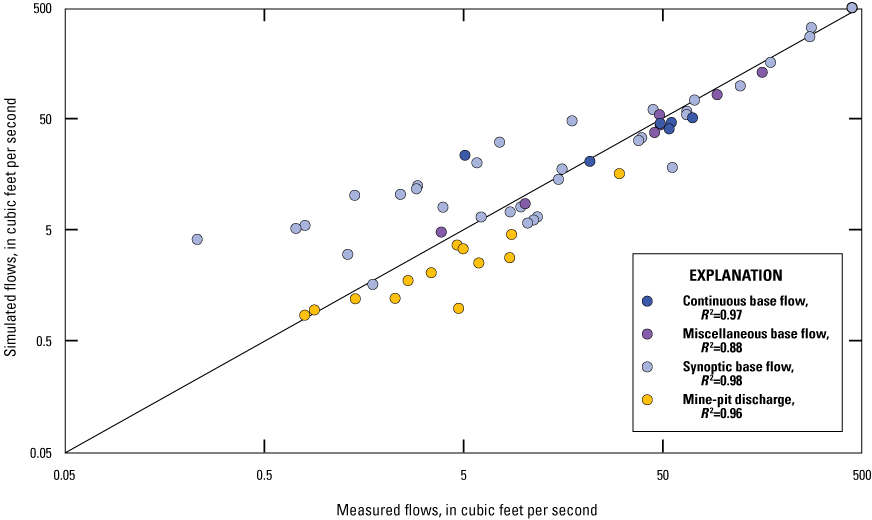
Measured and simulated base flow and mine-pit discharge differences in the mining model, northeastern Minnesota.

Measured and simulated streamflow and mine-pit discharge differences in the mining model, northeastern Minnesota.
Wetland Presence/Absence
The calibrated mining model was able to reproduce 71 percent of the mapped permanent wetland areas in the IRMA (white area divided by white plus orange area on fig. 19). The model produced 997 mi2 of wetlands (white plus green areas on fig. 19, defined as areas where the water table is within 1 ft of land surface), 71 percent of which overlap with mapped permanent wetlands (fig. 19 white areas equaling 658 mi2). This amount is 108 percent of actual wetland in the IRMA. The model produced 339 mi2 of permanent wetlands where they are not mapped (green areas on fig. 19; false-positive areas). Most of the areas where the model incorrectly produced wetlands are in the southeast part of the St. Louis River Basin in areas between the mapped wetlands and rivers. This suggests that the water table is too high near rivers, perhaps indicating that the hydraulic conductivity of surficial materials is too high or perhaps that these riparian wetland areas are not correctly mapped as wetlands, possibly because they are seasonal or because they do not support the plants used to identify wetlands. Large areas where the model was unable to produce wetlands occur in the northern part of the IRMA (orange area on fig. 19; false-negative areas). Surficial sediments are very thin (less than a few feet thick) over much of this area. The model likely has difficulty producing heads high enough to produce wetlands in bedrock near the land surface because the hydraulic conductivities of these rocks are calibrated in areas where they are buried beneath tens to hundreds of feet of glacial sediments. The PEST parameter for wetland area was effective for total wetland area produced by the model but not where those wetlands were produced.
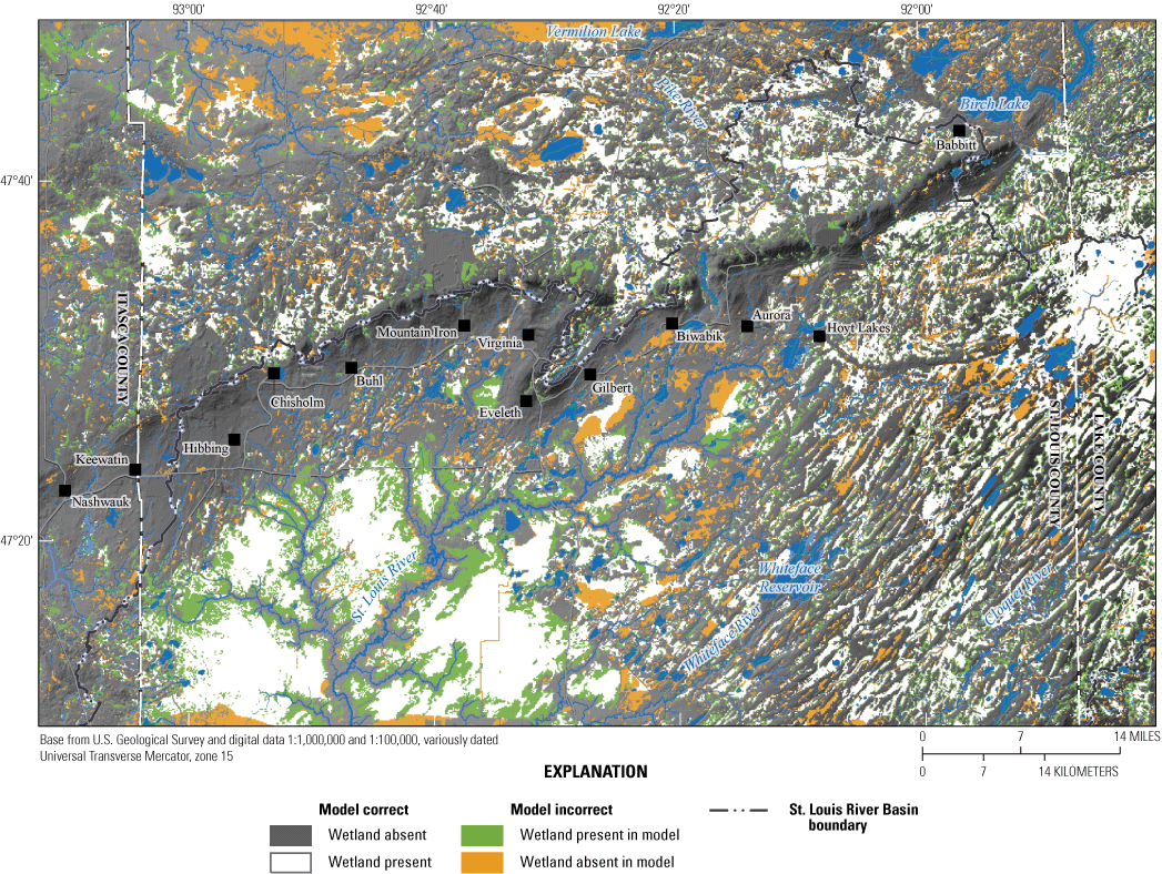
Locations of correctly and incorrectly simulated and actual wetlands in the mining model, northeastern Minnesota.
Well Withdrawals
Municipal (including commercial) well withdrawals account for 0.2 percent and mining process (other mining) well withdrawals account for 0.4 percent of the total modeled groundwater flow in the IRMA. However, the model simulated only 38 percent of specified municipal pumping and 60 percent of specified other-mining pumping. Three wells simulated no water pumped at all because they were open to model cells that were dry. The MODFLOW version used for these simulations reduces pumping rates specified by the user if the aquifer cannot support the specified rate. Because the specified pumping rates are self-reported by water users, this discrepancy could be a result of inaccurately reported pumping rates. Alternatively, errors in model properties controlling flow in the vicinity of these wells could also result in simulated pumping being lower than reported pumping. Requiring that the model produce specified rates of withdrawal could be used as a calibration target for future modeling (for example, Parsen and others, 2016), if pumping were an important model objective for the model. Municipal, commercial, and industrial pumping is not the focus of this study and accounts for less than 1 percent of the total groundwater flow in the model.
Calibrated Parameters
Hydraulic-conductivity zones calibrated using pilot points produced zones of varying heterogeneity. The most heterogeneous bedrock zones were the Biwabik Iron Formation (hydraulic-conductivity range: 2.6–25 ft/d) and crystalline bedrock (hydraulic-conductivity range: 0.9–20 ft/d), in the uppermost bedrock model layer (layer 5; table 6). Fractures density and aperture are known to be greatest in the uppermost parts of bedrock in the IRMA and lessen with depth (M. Jirsa, MGS, written commun., January 30, 2018). Hydraulic-conductivity variability of the Biwabik Iron Formation is large because of high concentrations of vugs in some areas relating to its metasedimentary origins (Morey, 1972; M. Liljegren, MN–DNR, oral commun., 2018).
Although the calibrated model hydraulic conductivities generally simulated water levels well, hydraulic conductivities in mine-related zones likely are too high because their simulated heads are too low (yellow and red dots below the 1:1 line, fig. 15). Further, the hydraulic conductivity of the Biwabik Iron Formation and the overlying coarse-grained glacial deposits, which supply water to mine pits, are particularly heterogeneous. The density of pilot points in these hydraulic-conductivity zones likely are inadequate to capture their real-world variability.
In glacial sediments, the most heterogeneous hydraulic-conductivity zone was Rainy Lobe sands and gravels (range: 0.8–28 ft/d, table 6). Generally, water levels from wells screened in glacial sediments had small head errors (lie close to the 1:1 line, fig.15). Most large residuals in glacial sediments are negative (modeled less than measured head), suggesting that calibration was unable to produce hydraulic conductivities high enough in some areas (fig. 15). Each of the 29 hydraulic-conductivity zones had calibrated vertical hydraulic-conductivity anisotropy. The largest anisotropies are in tailings basins (167 times less than horizontal hydraulic conductivity) and St. Louis Sublobe sand and gravel (225 times less than horizontal hydraulic conductivity). There is no trend in vertical hydraulic-conductivity anisotropy with depth in bedrock, However, because horizontal hydraulic conductivity in bedrock decreases with depth by about an order of magnitude per model layer, and because vertical hydraulic-conductivity anisotropy varies less than an order of magnitude in each bedrock unit, calibrated vertical hydraulic conductivity also decreases with depth.
The potential areal recharge array was divided into upland areas and wetland areas, each with their own multiplier (fig. 10). The wetland-area potential-recharge array multiplier was 1.1 (75 percent of the upland-area multiplier), likely reflecting the large amount of rejected recharge from the high water table in wetland areas. In a sense, the wetland-area recharge array multiplier has the effect of controlling the amount of rejected recharge. Because 20 percent of this rejected recharge is added to streamflow, the wetland-area recharge multiplier has the effect of reducing model error for stream base flow measurements. The upland-area potential-recharge multiplier was 1.5, indicating that the SWB recharge estimates were too small to produce the amount of groundwater flow through the model needed for base flow in streams in that area. Recharge multipliers equal to 1.0 would represent no change from the initial SWB potential areal recharge values. These calibrated multipliers are not equal to 1 because the groundwater model contains more complete hydrologic processes than does the SWB model. Calibrated streambed and drainbed conductance were nearly the same as the initial conductance, indicating that initial values for these parameters were appropriate for the system modeled. The model is most sensitive to the potential areal recharge multipliers.
Limitations and Assumptions of the Mining Model
Like all models of the natural environment, the steady-state mining model is a simplification of a complex and dynamic hydrogeologic system. The simplifications are dependent on the questions that the model is designed to answer. The mining model is intended to simulate regional groundwater flow in the IRMA. The model is not able to accurately simulate groundwater flow in small areas, especially near features like mine pits, which can have large hydraulic gradients. When compared with results from a pre-mining-scenario model of similar regional scale, mining-model results can indicate and quantify the hydrologic effects of mining in the IRMA. The regional model also is useful for providing lateral-boundary flows to future site-scale inset models but cannot answer site-scale questions (like those at a mine site or production well) directly.
Model Scale, Discretization, and Parameterization
This model broadly describes conditions across 3,205 mi2 of the IRMA, including the upper St. Louis River Basin along the Iron Range. Hydrogeologic materials were assumed to be horizontally isotropic, but with vertical anisotropy. Model cells are 400 ft×400 ft square and range in thickness from less than 1 to 800 ft. Cells of this size may be too large to accurately answer some question at a small scale, such as the details of groundwater interactions with surface waters. Like all finite-difference models, spatial input and model results (such as the lidar land-surface elevation, glacial stratigraphy, bedrock-surface elevation, groundwater heads, and flow paths near mine pits) are averages over the model cell area. Modeled groundwater heads, for example, may be shallower than the actual heads in places where groundwater gradients change over a small distance, such as near streams, wells, and mine pits. Near these features, modeled heads likely are too high. The bedrock-surface raster, which is coarser than land-surface DEM, also was averaged across each model cell, resulting in a model bedrock surface that was above the model land surface in some areas, particularly in areas where bedrock was at or near the land surface. To correct this, the model bedrock surface was adjusted to be no higher than 1 ft below the model land surface. Pilot points used to interpolate hydraulic-conductivity fields in many zones were widely spaced (at least 32,000 ft; 80 model cells) because of the few measured heads available. The resulting calibrated hydraulic-conductivity fields produced during calibration cannot represent actual hydraulic-conductivity variability. In hydrostratigraphic units that had very few observations, the hydraulic conductivity was calibrated as a zone, where one value is applied throughout the zone. In reality, hydraulic conductivity varies throughout the zone.
Groundwater flows preferentially through coarse-grained zones in unconsolidated sediments and through fractures and vugs in bedrock. While MODFLOW’s assumption of porous-medium flow is appropriate at the regional scale of the IRMA, this assumption is less appropriate at the small scale of a mine-pit wall, for example, where flow is likely dominated by fracture flow or flow through vugs. Analyses of model results that depend on groundwater-flow paths and flow times (well capture-zone delineation or groundwater travel times) likely are inappropriate where preferential groundwater-flow paths may be present. Because all model materials are assumed to be horizontally isotropic, modeled flow paths and flow times are likely inaccurate in materials that are anisotropically fractured or deposited.
Steady State
The results of the IRMA model represent unvarying average conditions and cannot provide information about the temporal dynamics of groundwater flow and heads. The potential areal recharge array specified in the model is an average during 1995–2015 (model steady-state period) and is the average condition represented in the mining model. Water levels and streamflows used in calibrating the model were measured during different periods. Calibration heads were measured during 1900–2017, with 97 percent of these measured after 1969 and 57 percent measured during the steady-state period. Calibration flows from continuous streamgages were averaged over a shorter period: 2012–15, corresponding to the years where the largest number of streamgages were active to provide a spatially consistent dataset. Flows measured outside this period were adjusted to represent flows during 2012–5. Precipitation during the calibration flows period was close to (6 percent higher than) that of the 1995–2015 average. Model results will be less accurate during times when general climatic and weather conditions are far different from those during the model steady-state period or if hydrologic temporal stationarity cannot be assumed (for example, under climate change scenarios).
Many hydrologic stresses (for example, mine-pit dewatering stage, tailings-basin pool stage) in the mining model required an elevation, which was determined from lidar DEMs measured in 2011. To ensure consistency with these elevations, municipal well and mine-pit dewatering withdrawal rates used in the model were those reported in 2011. However, 2011 was quite dry: precipitation at Aurora, Minnesota, near the center of the IRMA, was 78 percent (5.91 in.) lower than the 1995–2015 average. The use of 2011 lidar elevations resulted in hydrologic-stress stages that are too low for the steady-state period modeled. Model results are dependent on these stages in complex ways. For example, lower mine-pit DRN stage would tend to produce higher groundwater gradients to the mine pits, increasing mine-pit discharge. This is because mine-pit water levels, at least initially, will fall faster than adjacent groundwater levels, increasing discharge to the mine pits. This discharge routed to streams would produce higher simulated base flows for calibration. A model calibrated to these higher base flows may produce lower calibrated hydraulic conductivities in aquifers discharging to streams. The precipitation mismatch between the 1995–2015 model period and the 2011 hydrologic-stress stages should be considered when interpreting model results.
Hydrologic Stresses and Boundary Fluxes
The MODFLOW packages chosen to represent mining features, surface-water bodies, and wetlands in the mining model imply assumptions and create limitations for the results of the model. Dewatering from mine pits was represented using drains (DRN package), which can only remove water from aquifers. The amount of water removed from mine pits through drain stresses is controlled by the hydraulic gradient and the drain hydraulic conductivity, which is a calibrated parameter. Reported mine-pit dewatering flows were calibration targets and were aggregated and routed to downstream base flow targets. Reported flows from mine pits were assumed to reflect actual dewatering flow rather than permitted withdrawal rates and to lose no water in transit through evapotranspiration or other mechanisms on its path to a streamgage. Flows into and out of tailings basins are poorly constrained by calibration measurements. These flows were represented with the GHB package stresses, which define a groundwater head above which water will flow out of a model cell into a tailings basin and below which water will flow into a model cell out of a tailings basin. The assumption is that the tailings basin can supply an unlimited amount of water to the model cell in response to the downward gradient. This flow is controlled by the head gradient and the GHB conductance, which was estimated on the assumptions that the bed sediments of a tailings basin are fine grained and poorly compacted. The assumed conductance value corresponds to a hydraulic conductivity of 0.1 ft/d and a bed-sediment thickness of 1 ft. The conductance is uncalibrated because the flows into or out of tailings basins to groundwater are unmeasured. At this conductance, tailings basins supply 2.7 percent of flow into groundwater in the mining model.
Wetlands are not explicitly modeled using a hydrologic stress in the mining model because wetlands cover 29 percent of the IRMA, and to do so may over-constrain the modeled heads. Wetlands are assumed to be any area where groundwater levels are within 1 ft of land surface. If the UZF package had not been used to model wetlands, the elevation of the simulated water table would have been constrained in these areas. Thus, the groundwater head field would have been distorted to force groundwater discharge that actually terminates as seepage at wetlands to discharge to downgradient stream channels instead. Such groundwater discharge to streams in the large wetland areas of the IRMA would have artificially increased modeled streamflow and lowered aquifer hydraulic conductivity to prevent cell flooding.
Fractions of the water flux simulated as rejected recharge (20 percent) or as surface seepage (80 percent) were aggregated as runoff and routed to streamgages, augmenting modeled base flow for calibration purposes. These assumed runoff percentages were based on a water balance study in a wetland-rich area of northwestern Minnesota (Cowdery and others, 2019) and were not calibration parameters. Finally, the UZF variable SURFDEP was assumed to be 1 ft based on the average land-surface undulations in wetlands in the IRMA. These UZF package assumptions, though realistic, affected the calibration of the model and should be kept in mind when interpreting or using the model results. See Feinstein and others (2020) for a more complete discussion of possible effects of SURFDEP.
The potential-recharge array used in the UZF package was made from two SWB models of different resolutions: one coarse statewide model and one higher resolution model of the St. Louis River Basin. The St. Louis River Basin SWB model used streamflows from that Basin in its calibration and as a result, the potential-recharge array is likely most accurate in this area. The potential-recharge array was multiplied by two calibrated factors: a factor for upland areas and a factor for permanent wetland areas, which were assumed to be coincident with mapped permanent wetlands from a coverage from MGS for St. Louis and Cook County and from the MN–DNR’s NWI mapped permanent wetlands for Itasca County. The unsaturated zone of permanent wetland areas is assumed to behave fundamentally differently than the unsaturated zone of uplands because unsaturated zones in the uplands are substantially thicker than those in wetland areas. This assumption justifies separate potential-recharge array multipliers. Finally, areas of open water have zero potential-recharge in SWB models, under the assumption that any water for recharge in these areas comes from the surface-water body. These assumptions likely are valid for regional groundwater flow in aquifers in the IRMA. However, in specific areas and at local scales, some of these assumptions may not be accurate.
Well withdrawals were modeled in the mining model using the MODFLOW MNW2 package. Lateral-boundary groundwater fluxes are supplied by the WEL package. Both packages will inject or extract the specified amount of water into the model at their cell locations. However, if these packages are specified to remove water from the model, they can only do so if the cells in which they are located retain some water. If a well stress removes so much water that a cell goes dry, the actual withdrawal specified in the model input file is reduced until the cell retains water. Collectively, MNW2 stresses could only produce 55 percent of the specified well withdrawals without cells drying out, although the withdrawal produced is variable among wells. This means that the modeled aquifers with calibrated hydraulic conductivities have lower hydraulic conductivities in the vicinity of wells than do the actual aquifers. Therefore, this model would be inappropriate to answer specific questions about specific wells. Lateral-boundary WEL stresses could only produce (remove) 68 percent of specified water without going dry. This means that the modeled aquifers could not transmit as much water in some areas compared to the real aquifers, implying that hydraulic conductivities are too low in modeled aquifers in those areas. For example, along the northwestern boundary of the model, streams become losing (red circles) at the model edge (fig. 14). In these cells, the aquifer cannot supply the specified WEL withdrawals, so water is induced to flow out of streams to supply some of the water. Model results in the vicinity of these unsatisfied WEL stresses are likely not reliable. However, because MNW2 and WEL stresses account for less than 5 percent of model flows, these problems likely have a small effect on the regional results of the mining model as a whole. The boundary flows were derived from the results of a 1-layer analytic-element model`. Flow differences can be expected between this simple 1-layer model and the complex, multilayer IRMA model.
Representativeness of Heads Used for Calibration
Not only are model calibration heads limited temporally, they are also limited by their spatial extent and ability to represent all geologic material in the IRMA. Wells and the data that they provide (hydraulic conductivities from aquifer/specific capacity tests, measured groundwater heads) are not evenly distributed spatially or among aquifers. Wells are drilled where water is needed, available, or where water levels or samples are needed. Water is needed near residential, commercial, and industrial development (mainly mines and surrounding infrastructure in the IRMA). Water is available in more productive aquifers or the more productive parts of them. More transmissive parts of hydrologically heterogeneous aquifers, like the Biwabik Iron Formation, are more likely to have water wells drilled in them. This bias likely results in hydraulic-conductivity estimates being higher than the average part of the aquifer actually is. Water levels from wells are then skewed to the more productive parts of aquifers where water and water data are needed. Additionally, water levels can be skewed by imprecise measurement. Nearly all of the water levels used in model calibration were measured by well drillers when the well was drilled. These measurements are often poorly located, rounded to the foot, and often do not account for the measuring point height above the ground, thus skewing water-level depths (R. Barnes, University of Minnesota and others, written commun., 2019).
Even with the limitations of the mining model, regional analyses of model results are valid and appropriate. An example of appropriate analysis is regional comparisons of the spatial patterns of groundwater flows and heads in the mining-model with those patterns in the pre-mining model (described below). However, comparisons of these results in specific areas, especially near mining features, are inappropriate because of the model limitations described previously. Another example of appropriate use of model results is using mining-model groundwater flows as specified boundary flows in another model inset in the IRMA. Care must be exercised when constructing inset models to ensure that the effects of hydrologic stresses within the inset model do not propagate to the specified flow boundaries. Other uses of the mining model are inappropriate given the model limitations. In particular, using the model to evaluate site-specific hydrologic stresses (like a new mine pit) may not produce valid results because the scale of the added stress is too small in a regional model. Such scenarios are more appropriately explored with an inset model bounded by flow from the mining model.
Pre-Mining Scenario Model
A pre-mining scenario model was constructed to quantify the hydrologic changes in the model area produced by iron mining. These changes were determined by subtracting the results of the pre-mining model from those of the mining model. The pre-mining scenario model was developed using the calibrated mining model as a starting point; features of iron mining were then removed. The land-surface and bedrock topography were restored to their estimated original contours, and hydraulic conductivity was modified to reflect the original geologic materials. Hydraulic stresses representing mining features (for example, mine-pit dewatering) and municipal and industrial well withdrawals were removed. An archive of all model input, output, executable, and ancillary files is at https://doi.org/10.5066/P9U6KSBJ (Cowdery and others, 2023).
The original surficial topography of the Iron Range was provided by the MGS (Lively and others, 2002, 200529) based on original survey maps produced in 1899 and 1900. This topography was substituted for the land surface (top of model layer 1) in the area available (fig. 20). Vertical offsets at the boundary of the substituted area were smoothed by calculating and substituting three-cell spatial averages in a three-cell rim around the substituted area. This produced a pre-mining land-surface topography estimate that was higher in areas of mine pits and lower in areas of waste-rock piles and tailings basins (figs. 20, 7, and 9) compared with the mining model. Note that several large tailings basins are outside of MGS pre-mining land-surface topography area. These basins remain in the pre-mining model land-surface topography because no data for the original topography exist. Bedrock-surface topography is the same as the mining model’s, except that mine pits from the 2011 lidar DEM were not included. The method for determining model layer thickness was the same as that used in the mining model except the pre-mining land and bedrock surfaces were used. Surficial and glacial sediment model layers (1–4) are uniform in thickness below land surface until truncated by the bedrock surface. Bedrock model layers (5–8) are uniform in thickness below the bedrock surface (table 1).
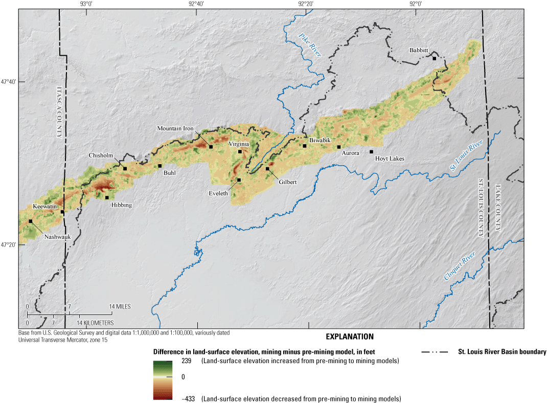
Difference of land-surface elevation between mining and pre-mining models, northeastern Minnesota.
The hydraulic conductivity of mining-related zones (mine pits, waste-rock piles, mining-disturbed areas, and tailings basins) in the mining model (fig. 7) were replaced with the calibrated hydraulic conductivity of the original geologic materials (fig. 21 for model layer 1) as reconstructed by Jennings and Reynolds (2005). In layers 1–4, cells with mining features were assigned model-calibrated surficial and glacial hydraulic conductivities. The overall effect of these modifications likely is modest because bedrock is close to the surface over most of the Iron Range and surficial sediments are thin. In zones where pilot points produced hydraulic conductivity fields (layers 2–4), the average hydraulic conductivity of each material in each model layer was calculated as an average of the hydraulic conductivity in nearby cells of the same material. This average material zone hydraulic conductivity was then assigned to mining-related zones in the pre-mining model based on the Jennings and Reynolds (2005) reconstruction. In bedrock layers 5–8, only the Biwabik Iron Formation in mine pits were replaced. Average zone hydraulic conductivities for the Biwabik Iron Formation in each layer, calculated like those for glacial and surficial sediments mentioned previously, were substituted in mine pits.
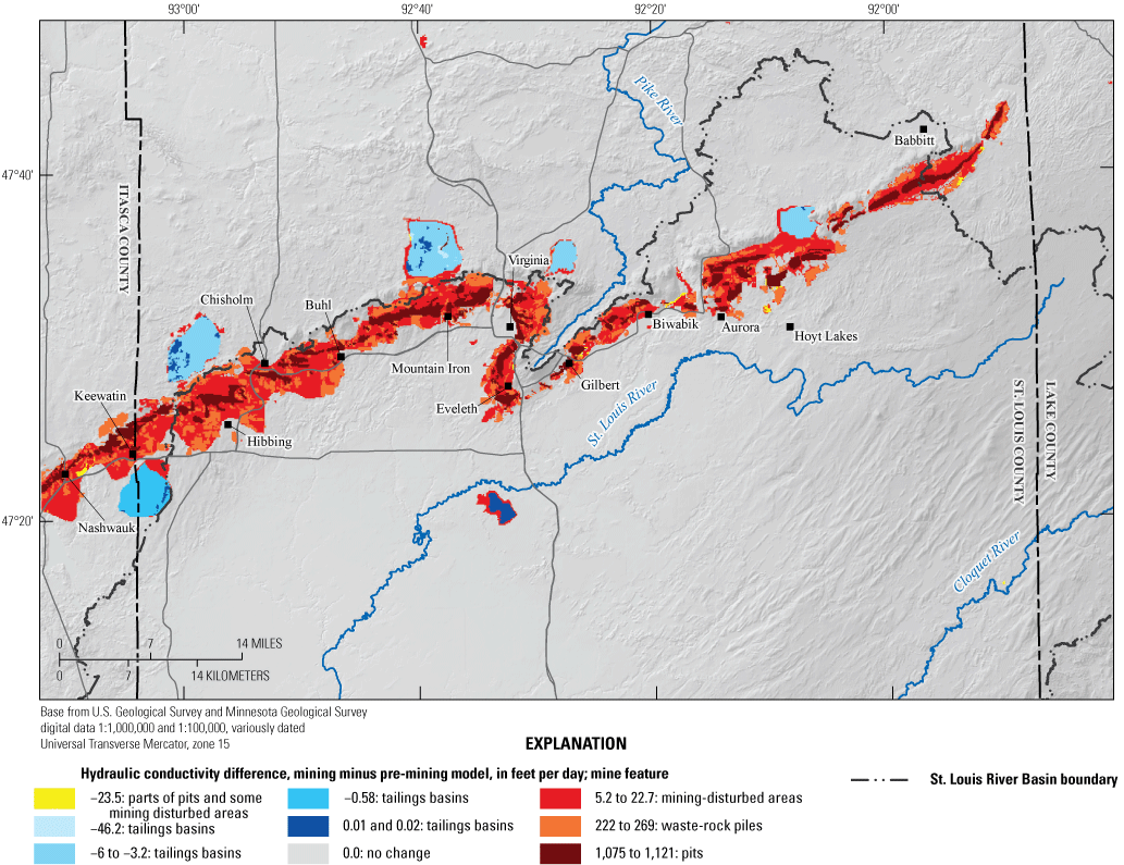
Differences in hydraulic conductivity of layer 1, mining minus pre-mining models, northeastern Minnesota.
A process like that used to adjust pre-mining model hydraulic conductivity adjusted the potential-recharge array for the pre-mining model. This adjustment was necessary because potential-recharge is zero over open water such as mine-pit lakes, which were removed from the pre-mining model. The mining model potential-recharge array was used as a base for the pre-mining model potential-recharge array, including the upland and wetland multipliers. The average potential-recharge rate was calculated in the same manner as average hydraulic conductivity for each reconstructed original geologic material in the mining-related zones of the mining model. Average potential-recharge rates for the materials that would have occurred in the mining areas was substituted for the rates from the mining model.
All mining-related hydrologic stresses in the mining model were removed, including DRN stresses used to simulate mine-pit dewatering, GHB stresses used to simulate tailings-basin interactions, and permitted well withdrawals (MNW2 stresses; fig. 22). No stream reaches or lakes were added to the pre-mining model because pre-mining stream and lake data were not available electronically. On paper maps of pre-mining topography and hydrology, no changes in hydrography were readily evident. Elevations of stream reaches (simulated using the SFR2 package) and lakes (simulated using the RIV package) were changed to correspond to the new topography of the pre-mining model where land-surface elevation changed. However, the SFR2 stream-reach errors near mine pits in the mining model were not corrected in this process.
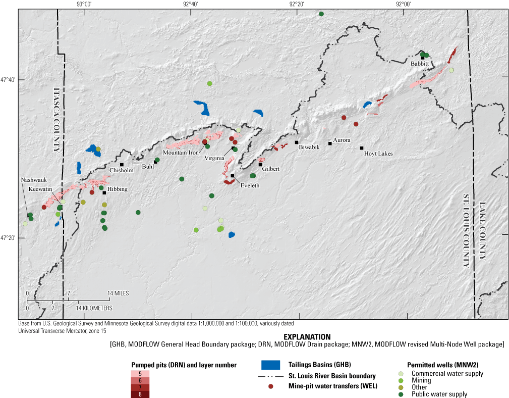
Mining-related hydrologic stresses removed from the mining model to produce the pre-mining model, northeastern Minnesota.
Limitations and Assumptions of the Pre-Mining Scenario Model
Because the mining model was used as the basis for the pre-mining model, the limitations and assumptions of the mining model apply to the pre-mining model, except for those related to mining features, including all permitted water use. The comparison of the two models to estimate hydrologic changes from iron mining assumes that mining is the only important change in hydrology in the IRMA between the two periods. Assumptions also were required to reconstruct pre-mining land surface, geology, and surface hydrology. No actual pre-mining maps of the land surface were available; maps of the Iron Range used to reconstruct the land surface in the pre-mining model were made during 1899–1900 after some mining began and do not cover the entire area affected by iron mining. In particular, the land surface of large tailings basins far from the mapped area could not be corrected to its pre-mining topography. This lack of topography resulted in tailings-basin areas in the pre-mining model that are topographically too high. The hydraulic conductivity and potential recharge in tailings-basin areas were changed to reflect geologic materials likely there originally, however. Topographic changes from town and city development outside the pre-mining topographic maps present similar problems, although the changes are smaller. Surface waters above and immediately adjacent to the mines were obliterated during mining and were not restored in the pre-mining model, even though pre-mining topographic maps include surface waters in and around the mine areas. The reason for this omission is because these areas were typically stream headwaters that were ephemeral or intermittent, thus did not warrant inclusion in the pre-mining model.
All mining features were assumed to be far enough from vertical model boundaries so that the effects of their removal would not propagate to the model boundaries. Therefore, flows through the vertical boundaries (Haserodt and other, 2019) were assumed to be the same in both models. These flows are the output of a large regional groundwater-flow model calibrated to modern conditions. The IRMA boundary was selected to be far from substantial modern development, so the assumption that flows through the vertical boundaries are the same in both models should not greatly limit interpretation of model results.
The potential-recharge array used in both models is based on SWB models, which have land use as one of their main variables (Smith and Westenbroek, 2015; Smith, 2017). The method used to produce the pre-mining potential-recharge array did not substitute pre-mining land uses into the SWB models and re-run them, producing new potential-recharge estimates. Instead, areas adjacent to mining features were spatially averaged and substituted into the pre-mining potential-recharge array. This choice has the effect of using a potential-recharge estimate based on modern nonmining land use in the pre-mining model. Because recharge is, by far, the greatest input flow into both groundwater models, care must be used when interpreting pre-mining model results, particularly the flows that it produces.
These limitations and assumptions introduce uncertainty into the results of the pre-mining model. However, the main use of the pre-mining model is to compare its results to that of the mining model to estimate the effect of mining on regional hydrology in the St. Louis River Basin. This comparison is done by subtracting the pre-mining model results from the mining results, producing a change between the two periods. As discussed in chapter 10 of Anderson and others (2015), the uncertainty of model forecasts formed as the difference between two model results is smaller than the uncertainty in the individual model forecasts because the subtraction removes the effects of systematic bias in the model results. For example, if the hydraulic conductivity of the Biwabik Iron Formation in model layer 8 is too high, effects of that error will not appear in the comparison of the two model results because that conductivity is identical in both models. In a similar way, complications that were not incorporated in the models can be ignored in the comparison of the results of the models. For example, no effort was made to quantify or incorporate the difference in climate between the mining-model period (1995–2015) and that of the pre-mining period, which was not defined beyond that it was sometime before mining. By assuming that the mining model and the pre-mining model operate under identical climates, any results that would have been affected by that different climate are eliminated in the comparison, leaving only effects caused by differences between the models: the hydrologic effects of mining features. Thus, this modeling is less suited to describe the actual difference in hydrologic conditions, which is the cumulative effects of mining and other changes (such as climate, agriculture, artificial drainage, and so forth) that occurred between the two periods.
Differences Between the Mining and Pre-Mining Model Results
The pre-mining model water table is nearly identical (within 0.1 ft) to that of the mining model except near mining features (figs. 23 and 24). In the cross-section A–A′, the pre-mining water table (light-blue line) slopes down from the Superior highlands in the east toward the Iron Range, rises at the Virginia Horn, descends into the Pike River Basin, rises at the Iron Range north of Buhl, and slopes down to the west (figs. 1 and 24). However, the pre-mining water table is hundreds of feet higher at and around future mine pits and is lower beneath some future waste-rock piles and tailings basins (western-most tailings basin in fig. 24) than in the mining model. Note, again, that topographic effect of several large tailings basins remains in the pre-mining model because the original land-surface topographic data do not exist. The hydrologic effects of the basins have been removed, however. Regional, deep pre-mining groundwater discharges to the Embarrass River (fig. 24) rather than to the McKinley mine pit as in the mining model (fig. 13). The regional low in groundwater head that occurs near the Missabe Mountain mine pit in the mining model (fig. 13) is absent in the pre-mining model (fig. 24), indicating that the flow to the north, south, or north and south (deep brown arrows, figs. 13 and 24) from the cross section in this area is induced by mine pits in the mining model. The regional lows in groundwater head beneath Virginia and somewhat to the west (piezometric-elevation contour 1,300, fig. 24) are nearly identical in both models, indicating that groundwater levels in these areas are driven by natural features like tributaries of the St. Louis River to the south, the headwaters of the Pike River, tributaries of the Little Fork River to the north, or some or all of these. Shallow groundwater flow is similar between models in the far west and east of the IRMA away from the Iron Range mining features.
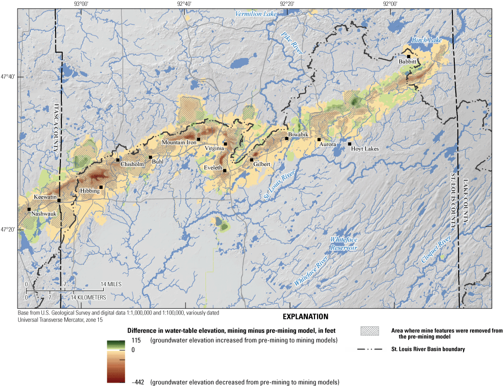
Simulated water-table elevation difference, mining minus pre-mining models, northeastern Minnesota.
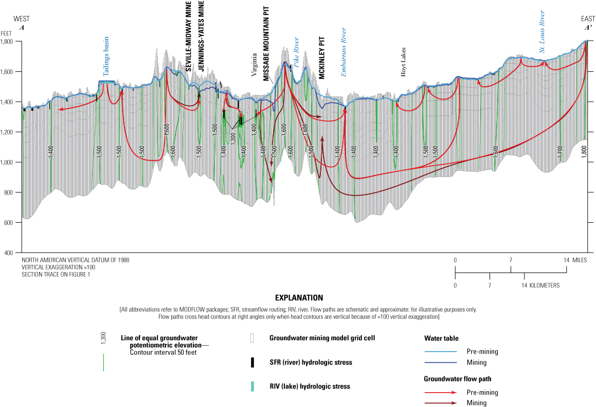
Pre-mining potentiometric contours and simulated water-table elevations and example groundwater flow paths from the mining and pre-mining models, northeastern Minnesota.
Changes in groundwater discharge to streams (fig. 25) from pre-mining to mining scenarios are also most pronounced near the mining features, but the discharge effects of mining extend farther than do changes in heads. Although groundwater flow (base flow) to streams increases by 2.1 percent because of mining (relative percent difference; green reaches, fig. 25), reaches where base flow decreases are more spatially extensive (red reaches). Base flow changes in streams can have important effects on riparian biota. For example, reductions in base flow may reduce the area where wild rice can grow (Pillsbury and McGuire, 2009). Notable changes in base flow far from iron mining features include base flow reductions to the ditches (straight, angular stream; slight base flow decrease) in the south-central part of the IRMA and mixed base flow change to small streams north of the Iron Range that exit the IRMA to the west. Mixed base flow changes to the St. Louis River occur in its middle reaches south of Aurora and Biwabik (see fig. 1 for town locations), whereas slight decreases occur in its lowest reaches in the IRMA. The area with the largest changes, mostly decreases in base flow, occur in stream headwaters nearest the Iron Range.
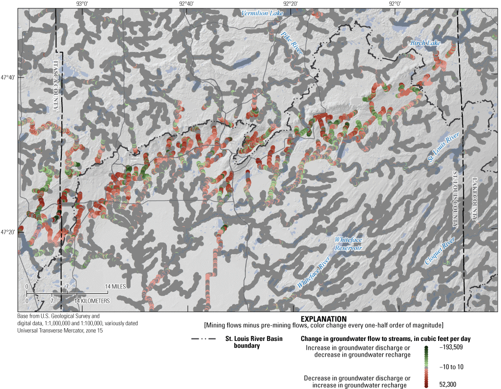
Differences in simulated steady-state groundwater flow to streams between mining and pre-mining models, northeastern Minnesota.
Water Balance
Effects of mining on groundwater flows in the IRMA were calculated by subtracting flows in the pre-mining model from flows in the mining model. Reductions in groundwater flows are negative and increases in flows are positive. Model results are separated by flows into groundwater (positive) and flows out of groundwater (negative). Adding these two flows together for each component of the water balance results in net flows into groundwater (table 12). Because all flows in the model are from the groundwater perspective, flows to and from the surface have opposite signs. For example, if groundwater flows to a stream (base flow), an increase in those flows is negative because that increase causes less water to remain in aquifers.
Table 12.
Net change in flows to groundwater resulting from mining in the model area, northeastern Minnesota.[Shaded cells (also marked with a *) are boundary conditions only in the mining model. MODFLOW, U.S. Geological Survey Modular Three-Dimensional Finite-Difference Ground-Water Flow model; ft3/d, cubic foot per day; WEL, MODFLOW Well package; MODFLOW RIV, River package; GW; groundwater; SFR2, MODFLOW Streamflow Routing package; %, percent; UZF, MODFLOW Unsaturated-Zone Flow package; LS, land surface; DRN, MODFLOW Drain package; GHB, MODFLOW General Head Boundary package; MNW2, MODFLOW Multi-Node Well package]
Flows through the many components of the groundwater balance are similar in the two groundwater models, except for those related to mining features. Total groundwater flow in the pre-mining model is 167.1 Mft3/d, 3.6 Mft3/d less than the mining model. Areal recharge is the largest component of flow into groundwater in both models but is slightly higher in volume and percentage of inflow in the pre-mining model (pre-mining model—134.6 Mft3/d and 81 percent, respectively; mining model—133.2 Mft3/d and 78 percent, respectively). The largest categories of groundwater flow out of the pre-mining model are the same as those in the mining model: streams and surface seepage (43 and 49 percent, respectively, in the pre-mining model, compared to 43 and 45 percent, respectively, in the mining model). Stream seepage from groundwater (base flow) is identical between the models (12 percent), but surface seepage (areal, to the land surface) is 3.6 percent higher in the pre-mining model. Lateral flows through the vertical sides of each model are nearly identical. Lateral outflows, represented in the model as pumping wells at the model boundary, are 1,281 ft3/d higher in the pre-mining model (table 12; a decrease of 0.1 percent of total groundwater flow).
The largest changes in flows from the pre-mining to the mining model (calculated as mining-model flows minus pre-mining flows, table 12) were mine-pit outflows (−2.8 percent of pre-mining groundwater inflows), reduced surface seepage (+2.7 percent), net increased recharge from tailings basins (+2.4 percent), and net decreased discharge to streams (−1.0 percent). Note that the amount of recharge to groundwater from tailings basins nearly offsets the amount of mine outflows (groundwater discharge, pumped from mine pits), though these offsets did not occur in the same places. Note also that mine outflow, most of which ends up in streams and appears as base flow, augments the net increase of groundwater discharge to streams (base flow). Again, changes do not occur in the same places.
The overall increase in groundwater flow through aquifers in the mining model comes mostly from tailings-basin recharge offsetting a decrease in areal recharge. The amount of groundwater recharge from tailings basins is unmeasured and thus associated parameters are uncertain. However, groundwater withdrawals for mine dewatering and municipal and industrial uses may induce more recharge from lakes and less discharge to streams and to the land surface, thereby increasing groundwater flow slightly.
Originally, the Iron Range was and now is topographically high and a recharge area (figs. 1, 12, and 24). When mine pits were carved into this high area, the mine pits became local groundwater discharge area, so recharge locally decreased, and the water table generally became somewhat deeper (fig. 23). This could locally reduce surface seepage and reduce wetland area near mine-pit areas (fig. 26).
Wetlands
The second largest change in groundwater flow from the pre-mining to the mining models is a 2.7 percent reduction in water seepage to the land surface (surface seepage), a percentage nearly as large as mine outflows (table 12). This seepage both represents discrete springs, often near streams, and diffuse discharge maintaining wetlands. From the pre-mining to the mining model, surface seepage decreased by 4.4 Mft3/d, corresponding to a decrease of more than 12,000 acres of wetlands. Most areas of wetland loss are near mining features (orange areas, fig. 26). The pre-mining model simulated mapped wetlands (71-percent agreement by area) about as well as the mining model. Simulated wetlands covered 20 percent of the IRMA in the pre-mining model, which is about 0.1 percent more area than was simulated as wetlands by the mining model. The mining-model simulated wetlands that the pre-mining model did not in small areas near mining features, indicating that local increases in recharge raised the water table in these areas.
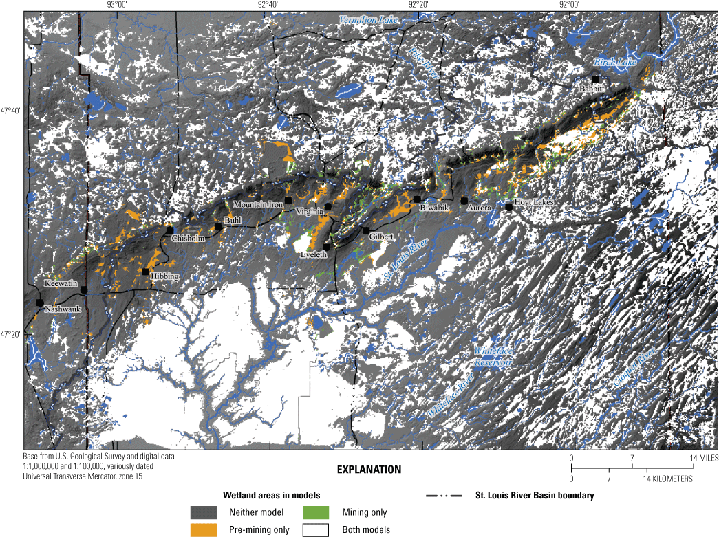
Differences in simulated wetland areas between the mining and pre-mining models, northeastern Minnesota.
Hydrologic Changes from Iron Mining
The mining and pre-mining models documented in this report show that iron mining has produced measurable hydrologic changes in the St. Louis River Basin, but that those changes occur mostly, and with the largest magnitude, near the mining features of the Iron Range. Mine pits affect hydrology in two main ways. First, mine pits increase the groundwater gradient when they are dewatered during mining (assuming other hydrologic conditions remain constant). The increased gradient drives groundwater discharge to the mine pits and lowers groundwater heads in their vicinity. Lower heads can increase groundwater recharge by decreasing the amount of rejected recharge simulated in the model. Lower heads can also decrease groundwater seepage to the land surface, reducing groundwater discharging to lakes and wetlands. Both mechanisms increase the amount of groundwater remaining in aquifers. Second, groundwater discharging to mine pits must be disposed of. In IRMA Iron Range mines, nearby streams receive much of this flow from mine pits. Mine dewatering augments base flow downstream from the receiving waters. This streamflow contribution from the mine-pit dewatering combined with the overall, though spatially variable, 2.1 percent increase in base flow to streams from iron mining, shows that mining causes some streams very near mine pits to have slightly higher base flows; an effect that decreases downstream. Some stream reaches lose base flow from mining (red reaches, fig. 25), however. The spatial distribution of these effects is hard to understand without modeling.
Mine pits that are flooded after mining has ceased have several local hydrological effects. Generally, mine pits with no natural outlet or mine pits that are not pumped for other reasons reach new equilibria with the surrounding groundwater. Mine pits can cause local losses of groundwater as water flows into them. Groundwater losses to mine pits may be partially offset by precipitation falling into mine-pits pools directly, which can initially recharge aquifers adjacent to mine pits that had been pumped during mining. The Biwabik Iron Formation offers substantial resistance to groundwater flow. A flooded mine pit carved out of the formation that turned into a mine-pit lake offers no internal resistance to water movement, however. The horizontal movement of groundwater entering a mine-pit lake on one side and exiting it on another is controlled by the lower hydraulic conductivity of the rocks composing the seepage faces of the mine-pit sides. However, within the mine-pit pool, water can move very quickly. Finally, flooded mine pits that have a water level lower than the water table in the pre-mining Biwabik Iron Formation will induce flow into the pits and lower the water table in the surrounding aquifers.
Tailings basins also affect local hydrology. Two features of these basins are hydrologically significant. First, these basins are typically lined with fine-grained sediments, and second, they have a pool over part of them during operation, which provides a constant supply of water at a head higher than the surrounding aquifer. The hydraulic conductivity of fine-grained tailings deposited on the bottom of basins often is higher than its grain size would suggest because its source rock, the Biwabik Iron Formation, is siliceous and not clay rich (Morey, 1972). Thus, tailings provide more resistance to flow relative to a surrounding sandy surficial aquifer, but less resistance relative to a more clay-rich till. Therefore, the hydrologic effect of tailings sediment depends on the natural sediment that they overlie. Many tailings basins were constructed in wetland basins whose sediments have lower hydraulic conductivity than do the tailings-basin sediments that overlie them. The net effect of the tailings basins in the IRMA is to increase groundwater recharge by 2.4 percent of total groundwater flow compared to the pre-mining model (table 12). Much of this recharge occurs in wetland-rich areas, so this recharge may have short flow paths, discharging to adjacent wetlands. Indeed, stream channels likely carrying this discharge are often seen in wetlands adjacent to tailings basins.
Waste-rock piles are the mining feature least likely to affect the hydrology in the IRMA. Generally, these are large piles of crystalline rock in large (one-tenth of a foot or larger) pieces. These piles provide very little resistance to water infiltration or flow. Precipitation that enters waste-rock piles quickly flows to the bottom where it enters natural sediments or flows laterally to pile edges. Simulated water tables suggest that some waste-rock piles can have groundwater levels as much as 20 ft higher than those of the pre-mining model. Discharge at the edge of waste-rock piles is likely, especially in low areas occupied by wetlands.
Changes in the areas of wetlands between the models are caused by complex hydrologic interactions of the mining features. The pre-mining model produces an additional 12,000 acres wetlands relative to the mining model, which are close to removed mining features (fig. 26). This area does not include possible wetlands that might originally have underlain tailings basins. Such wetlands could not be produced by the pre-mining model because the original topography of the tailings basins is unknown and was not restored. In the IRMA, many tailings basins are surrounded by mapped wetlands that are not simulated in the mining model, indicating that these areas may have been wetlands before mining began. The difference in wetland areas simulated in these models indicate that mining activities reduced groundwater-surface seepage by a net of 4.43 Mft3/d (table 12). This reduction is restricted to areas close to the mining features.
Summary
The U.S. Geological Survey built two regional three-dimensional MODFLOW steady-state groundwater-flow models to assess the changes to St. Louis River Basin hydrology from mining on the Iron Range in northeastern Minnesota. The U.S. Geological Survey collaborated in this study with bands of the Minnesota Chippewa Tribe, and the Minnesota Pollution Control Agency, all of whom are interested in this assessment to help them manage aquatic resources within the reservations and treaty-rights lands in the St. Louis River Basin. Comparison of the results of a mining model and a pre-mining model produced an estimate of the hydrologic changes that occurred from iron mining in the St. Louis River Basin near the Iron Range. The mining model was designed and calibrated to simulate regional groundwater heads and flows under 1995–2015 conditions. The pre-mining model was based on the mining model but had the land and bedrock surfaces and modeled mining features (mine pits, tailings basins, waste-rock piles, and mining-disturbed areas) restored to their pre-mining stratigraphic and hydrologic conditions. Many of the features important to the hydrology of this mining area (like individual mine pits) are difficult to represent in groundwater models and required use of hydrologic modeling tools outside of a groundwater-flow model to account for their effects. The difference between the results of the pre-mining model subtracted from the results of the mining model is a measure of the degree to which iron mining has affected hydrology in the Iron Range model area. These models represent regional groundwater hydrology, producing regional groundwater flows. The models are not capable of addressing site-specific questions. However, the modeled heads and flows can provide defensible boundary fluxes for local or site-specific groundwater-flow models constructed within the Iron Range model area.
Total groundwater flow in the mining model is 171 million cubic feet per day (table 8). Areal recharge is the largest source of groundwater in both the mining and pre-mining models (78 and 81 percent of total groundwater flow, respectively). Seepage from streams and lakes provides another 17 percent of total groundwater flow through both models. Water leaves aquifers through seepage to streams (discharge as base flow, 43 percent) and areal groundwater-surface seepage (45 and 49 percent, mining, and pre-mining models, respectively). A comparison of the mining and pre-mining model results shows that iron mining has produced measurable hydrologic changes in the St. Louis River Basin, and that most of those changes and the highest magnitude changes occur near the mining features. Overall, groundwater flow in the mining model was 3.62 million cubic feet per day (2.2 percent) greater than the pre-mining model total. This net increase was caused by an increase in recharge from tailings basins and a decrease in discharge from surface seepage. Groundwater discharge to mine pits was the largest change in groundwater flows between the models (2.8 percent of pre-mining model flow, table 12). Net recharge to groundwater from tailings basins (2.4 percent), net decrease in areal groundwater areal surface seepage (2.7 percent), and net increase in seepage to streams (1.0 percent) were also in the same percentage range. Groundwater lost through mine-pit withdrawals was nearly offset by groundwater gained through recharge from tailings basins. However, because losses and gains occurred in different areas, the effect of mining can have more substantial effects on local areas than the model-wide averages represent.
References Cited
AQUAVEO, 2018, GMS—Groundwater Modeling System (ver. 10.3): AQUAVEO modelling software accessed. 24 November 2020, at https://downloads.aquaveo.com/f.php5?s=gms&v=10.3&p=full64bit.
Barr Engineering Company, 2014, Hydrogeology of the fractured bedrock in the vicinity of the NorthMet Project: Barr Engineering Co., prepared for Poly Met Mining Inc., 112 p., accessed July 28, 2017, at http://files.dnr.state.mn.us/lands_minerals/northmet/water-approp/references/hydrogeology-fractured-bedrock-v3.pdf.
Berndt, M., and Bavin, T., 2009, Sulfate and mercury chemistry of the St. Louis River in Northeastern Minnesota—A report to the Minerals Coordinating Committee: Minnesota Department of Natural Resources, Division of Lands and Minerals, 80 p., accessed March 7, 2021, at https://files.dnr.state.mn.us/lands_minerals/reclamation/berndt_bavin_2009.pdf.
Cowdery, T.K., Baker, A.C., Haserodt, M.J., Feinstein, D.T., and Hunt, R.J., 2023, MODFLOW–NWT simulations of regional groundwater flow under mining and pre-mining scenarios near the Mesabi Iron Range within the St. Louis River Basin, northeastern Minnesota: U.S. Geological Survey data release, https://doi.org/10.5066/P9U6KSBJ.
Cowdery, T.K., Christenson, C.A., and Ziegeweid, J.R., 2019, The hydrologic benefits of wetland and prairie restoration in western Minnesota—Lessons learned at the Glacial Ridge National Wildlife Refuge, 2002–15: U.S. Geological Survey Scientific Investigations Report 2019–5041, 81 p., accessed May 31, 2022, at https://doi.org/10.3133/sir20195041.
Doherty, J., 2014, Addendum to the PEST manual: Brisbane, Australia, Watermark Numerical Computing, 45 p., accessed November 13, 2014, at http://www.pesthomepage.org/Downloads.php.
Doherty, J., 2010, PEST—Model-independent parameter estimation—User manual (5th ed.): Brisbane, Australia, Watermark Numerical Computing, 333 p., accessed November 13, 2014, at http://www.pesthomepage.org/Downloads.php.
Doherty, J., 2003, Groundwater model calibration using pilot points and regularization: Groundwater, v. 41, no. 2, p. 170–177. [Also available at https://ngwa.onlinelibrary.wiley.com/doi/10.1111/j.1745-6584.2003.tb02580.x.]
Doherty, J., and Hunt, R.J., 2010, Approaches to highly parameterized inversion—A guide to using PEST for groundwater-model calibration: U.S. Geological Survey Scientific Investigations Report 2010–5169, 59 p. [Also available at https://pubs.usgs.gov/sir/2010/5169/.]
Feinstein, D.T., Hart, D.J., Gatzke, S., Hunt, R.J., Niswonger, R.G., and Fienen, M.N., 2020, A simple method for simulating groundwater interactions with fens to forecast development effects: Ground Water, v. 58, no. 4, p. 524–534. [Also available at https://doi.org/10.1111/gwat.12931.]
Haserodt, M.J., Hunt, R.J., Cowdery, T.K., Leaf, A.T., and Baker, A.C., 2019, Simulation of the regional groundwater flow system in the St. Louis River Basin, Minnesota: U.S. Geological Survey Scientific Investigations Report 2019–5033, 41 p. [Also available at https://doi.org/10.3133/sir20195033].
Hobbs, H.C., and Goebel, J.E., 1982, Geologic map of Minnesota—Quaternary geology: Minnesota Geological Survey State Map Series S–01, 1 sheet, scale 1:500,000. [Also available at http://hdl.handle.net/11299/60085.]
Hunt, R.J., Doherty, J., and Tonkin, M.J., 2007, Are models too simple? Arguments for increased parameterization: Ground Water, v. 45, no. 3, p. 254–262. [Also available at https://doi.org/10.1111/j.1745-6584.2007.00316.x.]
Hunt, R.J., and Feinstein, D.T., 2012, MODFLOW–NWT—Robust handling of dry cells using a Newton Formulation of MODFLOW–2005: Ground Water, v. 50, no. 5, p. 659–663. [Also available at https://doi.org/10.1111/j.1745-6584.2012.00976.x.]
Institute of Hydrology, 1980, Low flow studies report no. 3—Catchment characteristic estimation manual: Wallingford, Oxfordshire, United Kingdom, Institute of Hydrology, 38 p. [Also available at https://nora.nerc.ac.uk/id/eprint/9098/.]
Jennings, C.E., and Reynolds, W.K., 2005, M–164—Surficial geology of the Mesabi Iron Range, Minnesota: Minnesota Geological Survey, 1 plate plus supplemental files, scale 1:100,000. [Also available at https://hdl.handle.net/11299/58160.]
Jirsa, M.A., 2016, OFR 16–4—Preliminary geologic maps of Lake and St. Louis Counties, northeastern Minnesota: Minnesota Geological Survey, 15 plates plus supplemental files, scale 1:100,000. [Also available at http://hdl.handle.net/11299/183258.]
Jirsa, M.A., Boerboom, T.J., Chandler, V.W., Mossler, J.H., Runkel, A.C., and Setterholm, D.R., 2011, Geologic map of Minnesota—Bedrock geology: Minnesota Geological Survey State Map Series S–21, 1 plate plus supplemental files, scale 1:500,000. [Also available at https://hdl.handle.net/11299/101466.]
Jirsa, M.A.; Bauer, E.J.; Boerboom, T.J.; Chandler, V.W.; Lively, R.S.; Mossler, J.H.; and Runkel, A.C., 2010, OFR10-02—Preliminary bedrock geologic map of Minnesota: Minnesota Geological Survey, 6 sheets plus supplemental files, scale 1:1,000,000. [Also available at http://hdl.handle.net/11299/98043.]
Kalman, D., 1996, A singularly valuable decomposition – The SVD of a matrix: The College Mathematics Journal, v. 27, no. 1, p. 2–23. [Also available at https://doi.org/10.1080/07468342.1996.11973744.]
King, K.E., 1980, History of drainage laws in Minnesota with special emphasis on the legal status of wet lands: University of Minnesota Water Resources Research Center Bulletin 106, 49 p. [Also available at https://conservancy.umn.edu/handle/11299/91295.]
Leaf, A.T., Fienen, M.N., and Reeves, H.W., 2021, sfrmaker and Linesink-Maker—Rapid construction of streamflow routing networks from hydrography data: Groundwater, v. 59, no. 5, p. 761–771. [Also available at https://doi.org/10.1111/gwat.13095.]
Leaf, A.T., Fienen, M.N., Hunt, R.J., and Buchwald, C.A., 2015, Groundwater/Surface-Water Interactions in the Bad River Watershed, Wisconsin: U.S. Geological Survey Scientific Investigations Report 2015–5162, 110 p. [Also available at https://doi.org/10.3133/sir20155162.]
Lively, R.S., Bauer, E.J., and Jirsa, M.A., 2005, M–157—Land-surface topography of the eastern half of the Mesabi Iron Range, northern Minnesota; 1899 and 1999: Minnesota Geological Survey, 3 plates, scale 1:100,000. [Also available at http://hdl.handle.net/11299/57695.]
Lively, R.S., Morey, G.B., and Bauer, E.J., 2002, M–118—One hundred years of mining: Alterations to the physical and cultural geography of the western half of the Mesabi Iron Range, northern Minnesota: Minnesota Geological Survey, 4 plates plus supplemental files, scale 1:100,000. [Also available at http://hdl.handle.net/11299/57178.]
McKay, L., Bondelid, T., Dewald, T., Johnston, J., Moore, R., and Rea, A., 2012, NHDPlus version 2—User guide: U.S. Environmental Protection Agency, prepared by NHDPlus, 95 p., 6 app., accessed June 16, 2020, at https://s3.amazonaws.com/edap-nhdplus/NHDPlusV21/Documentation/NHDPlusV2_User_Guide.pdf.
McKay, L.D., Cherry, J.A., and Gillham, R.W., 1993, Field experiments in a fractured clay till—Hydraulic conductivity and fracture aperture: Water Resources Research, v. 29, no. 4, p. 1149–1162. [Also available at https://agupubs.onlinelibrary.wiley.com/doi/epdf/10.1029/92WR02592.]
Minnesota Department of Natural Resources [MN–DNR], 2011, LiDAR elevation, Arrowhead Region, NE Minnesota, 2011: Minnesota IT Services Geospatial Information Office dataset, accessed June 2017 at https://resources.gisdata.mn.gov/pub/data/elevation/lidar/projects/arrowhead/.
Minnesota Department of Natural Resources [MN–DNR], 2016, Cooperative groundwater monitoring (CGM): MN–DNR web page, accessed May 27, 2016, at https://www.dnr.state.mn.us/waters/cgm/index.html.
Minnesota Department of Natural Resources [MN–DNR], 2018, National Wetland Inventory update for Minnesota: Minnesota Department of Natural Resources metadata, accessed November 6, 2018, at https://resources.gisdata.mn.gov/pub/gdrs/data/pub/us_mn_state_dnr/water_nat_wetlands_inv_2009_2014/metadata/metadata.html.
Niswonger, R.G., Panday, S., and Ibaraki, M., 2011, MODFLOW–NWT—A Newton formulation for MODFLOW–2005: U.S. Geological Survey Techniques and Methods, book 6, chap. A37, 44 p. [Also available at https://pubs.usgs.gov/tm/tm6a37/.]
Niswonger, R.G., and Prudic, D.E., 2005, Documentation of the streamflow-routing (SFR2) package to include unsaturated flow beneath streams—A modification to SFR1: U.S. Geological Survey Techniques and Methods, book 6, chap. A13, 50 p. [Also available at https://doi.org/10.3133/tm6A13.]
Siegel, D.I., and Ericson, D.W., 1980, Hydrology and water quality of the copper-nickel study region, northeastern Minnesota: U.S. Geological Survey Open-File Report 80–739, 87 p., 2 pls., accessed November 16, 2017, at https://conservancy.umn.edu/handle/11299/189248.
Smith, E.A., 2017, Soil-water-balance model data sets for the St. Louis River drainage basin, northeast Minnesota, 1995–2010: U.S. Geological Survey data release, accessed June 2018 at https://doi.org/10.5066/F7Z60MJ0.
Smith, E.A., and Westenbroek, S.M., 2015, Potential groundwater recharge for the State of Minnesota using the Soil-Water-Balance model, 1996–2010: U.S. Geological Survey Scientific Investigations Report 2015–5038, 85 p. [Also available at https://pubs.er.usgs.gov/publication/sir20155038.]
Tetra Tech, 2014, Upper St. Louis River watershed mining area hydrology: Minnesota Pollution Control Agency, prepared by Tetra Tech, 88 p., accessed December 14, 2017, at https://www.pca.state.mn.us/sites/default/files/wq-iw10-12p.pdf.
Thornton, P.E., Thornton, M.M., Mayer, B.W., Wilhelmi, N., Wei, Y., Devarakonda, R., and Cook, R.B., 2014, Daymet—Daily surface weather data on a 1-km grid for North America (ver. 2, May 2014): Oak Ridge, Tenn., Oak Ridge National Laboratory Distributed Active Archive Center digital data, accessed May 8, 2016, at https://doi.org/10.3334/ORNLDAAC/1219.
U.S. Geological Survey [USGS], 2022, USGS water data for the Nation: U.S. Geological Survey National Water Information System database, accessed November 2022 at https://doi.org/10.5066/F7P55KJN.
Wahl, K.L., and Wahl, T.L., 1988, Effects of regional groundwater level declines on streamflow in the Oklahoma Panhandle, in The Symposium on Water-Use Data for Water Resources Management, Proceedings: Bethesda, Md., American Water Resources Association, Technical publication series 88–2, p. 239–249.
Conversion Factors
U.S. customary units to International System of Units
Datum
Vertical coordinate information is referenced to the North American Vertical Datum of 1988 (NAVD 88).
Elevation, as used in this report, refers to distance above the vertical datum.
Abbreviations
DEM
digital elevation model
DRN
MODFLOW Drain package
ET
evapotranspiration
GHB
MODFLOW General Head Boundary package
IRMA
Iron Range model area
lidar
light detection and ranging
MODFLOW
U.S. Geological Survey Modular Three-Dimensional Finite-Difference Ground-Water Flow model
MGS
Minnesota Geological Survey
MN–DNR
Minnesota Department of Natural Resources
NWI
National Wetlands Inventory
MNW2
MODFLOW revised Multi-Node Well package
PEST
automated parameter-estimation software
RIV
MODFLOW River package
SFR2
MODFLOW revised Streamflow Routing package
SWB
Soil-Water-Balance model
USGS
U.S. Geological Survey
UZF
MODFLOW Unsaturated-Zone Flow package
For more information about this publication, contact:
Director, USGS Upper Midwest Water Science Center
1 Gifford Pinchot Drive
Madison, WI 53726
For additional information, visit: https://www.usgs.gov/centers/upper-midwest-water-science-center
Publishing support provided by the Rolla Publishing Service Center
Suggested Citation
Cowdery, T.K., Baker, A.C., Haserodt, M.J., Feinstein, D.T., and Hunt, R.J., 2023, Hydrologic change in the St. Louis River Basin from iron mining on the Mesabi Iron Range, northeastern Minnesota: U.S. Geological Survey Scientific Investigations Report 2022–5124, 59 p., https://doi.org/10.3133/sir20225124.
ISSN: 2328-0328 (online)
Study Area
| Publication type | Report |
|---|---|
| Publication Subtype | USGS Numbered Series |
| Title | Hydrologic change in the St. Louis River Basin from iron mining on the Mesabi Iron Range, northeastern Minnesota |
| Series title | Scientific Investigations Report |
| Series number | 2022-5124 |
| DOI | 10.3133/sir20225124 |
| Year Published | 2023 |
| Language | English |
| Publisher | U.S. Geological Survey |
| Publisher location | Reston, Va. |
| Contributing office(s) | Upper Midwest Water Science Center |
| Description | Report: viii, 59 p.; 2 Data Releases |
| Country | United States |
| State | Minnesota |
| Other Geospatial | Mesabi Iron Range, St Louis River basin |
| Online Only (Y/N) | Y |
| Google Analytic Metrics | Metrics page |