

Linear Regression Model Documentation for Computing Water-Quality Constituent Concentrations or Densities Using Continuous Real-Time Water-Quality Data for the Kansas River above Topeka Weir at Topeka, Kansas, November 2018 through June 2021
Links
- Document: Report (5.44 MB pdf) , HTML , XML
- Appendix: Appendixes 1–14 (pdf)
- Dataset: USGS National Water Information System database —USGS water data for the Nation
- Download citation as: RIS | Dublin Core
Acknowledgments
The author thanks the Kansas Water Office, the Kansas Department of Health and Environment, The Nature Conservancy, the City of Lawrence, the City of Manhattan, the City of Olathe, the City of Topeka, WaterOne, and Evergy for a beneficial and lasting partnership in monitoring water-quality conditions in the Kansas River.
The author thanks U.S. Geological Survey technical reviewers Teresa Rasmussen (Lawrence, Kansas), Kyle Juracek (Lawrence, Kans.), Mandy Stone (Lawrence, Kans.), and Tim Hoffman (Troy, New York) for reviewing previous drafts of this report. The author also thanks U.S. Geological Survey geographer Diana Restrepo-Osorio for assistance in adjusting the study area map to fit the needs of this report. Lastly, this report would not have been possible without the hard work by past and present U.S. Geological Survey staff at the Kansas Water Science Center who assisted with data collection, analyses, and project and database management.
Abstract
The Kansas River and its associated alluvial aquifer provide drinking water to more than 950,000 people in northeastern Kansas. Water suppliers that rely on the Kansas River as a water-supply source use physical and chemical processes to treat and remove contaminants before public distribution. An early-notification system of changing water-quality conditions allows water suppliers to proactively make decisions that affect water treatment. The U.S. Geological Survey (USGS), in cooperation with the Kansas Water Office (funded in part through the Kansas Water Plan), the Kansas Department of Health and Environment, The Nature Conservancy, the City of Lawrence, the City of Manhattan, the City of Olathe, the City of Topeka, WaterOne, and Evergy, began collecting water-quality data at the Kansas River above Topeka Weir at Topeka, Kansas (USGS site 06888990, hereafter referred to as the “Topeka site”), during November 2018 to develop linear regression models that relate continuous in situ water-quality sensor measurements to discretely sampled water-quality constituent concentrations or densities. The addition of the Topeka site expanded an existing water-quality monitoring network, which included the upstream Kansas River at Wamego, Kans., and downstream Kansas River at De Soto, Kans., sites. Linear regression analysis was used to develop models that compute real-time concentrations or densities for total dissolved solids, major ions, hardness as calcium carbonate, nutrients (nitrogen and phosphorus species), chlorophyll a, total suspended solids, suspended sediment, and Escherichia coli at the Topeka site using data collected during November 2018 through June 2021. Water-quality constituent concentrations or densities computed from the models documented in this report are available at the USGS National Real-Time Water-Quality website (https://nrtwq.usgs.gov), are useful to the public for cultural and recreational purposes, and can be used to guide water-treatment processes, compare conditions with Federal and State water-quality criteria, and characterize changes in Kansas River water-quality conditions through time.
Introduction
Water suppliers use the Kansas River and its associated alluvial aquifer to supply drinking water to more than 950,000 people throughout northeastern Kansas (Josh Olson, Kansas Water Office, written commun., July 21, 2022). Other uses of the Kansas River include cultural and recreational, industrial, food procurement, aquatic-life support, groundwater recharge, irrigation, and livestock water use (Kansas Department of Health and Environment, 2011). Water suppliers that rely on the Kansas River as a water-supply source use numerous physiochemical processes to treat and remove contaminants from the water before distribution. Water-quality characteristics of the source water determine the treatment processes used by water suppliers to effectively remove contaminants. An early-notification system of changing water-quality conditions near water-supply intakes allows water suppliers to proactively make decisions that affect water treatment. The water-quality data used to develop this early-notification system can also be used to characterize water-quality conditions in the Kansas River over time.
Concomitant continuous in situ water-quality monitoring and discrete water-quality sampling in the Kansas River began during July 1999 primarily to characterize water-quality conditions by developing regression models using a combination of continuous water-quality monitor data and discrete water-quality samples to compute continuous concentrations or densities of water-quality constituents that are not easily measured in real time (Rasmussen and others, 2005). As part of this initial effort, regression models that computed concentrations or densities of major ions, nutrients, sediment, fecal indicator bacteria, and trace elements at sites near Wamego, Topeka, and De Soto, Kansas, during July 1999 through September 2005 were developed (Rasmussen and others, 2005).
Kansas River water-quality sampling resumed after upstream releases from Milford Lake (a reservoir that contributes streamflow to the Kansas River) during a toxic cyanobacterial event in August 2011 to primarily characterize transport of cyanobacteria, cyanotoxins, and associated taste-and-odor compounds from upstream reservoirs to the Kansas River (Graham and others, 2012). After the Milford Lake release event, continuous and discrete water-quality monitoring resumed at the Kansas River at Wamego (U.S. Geological Survey [USGS] site 06887500; hereafter referred to as the “Wamego site”) and De Soto (USGS site 06892350; hereafter referred to as the “De Soto site”), Kans., sites in July 2012 to characterize water-quality conditions, including cyanobacteria and associated toxins and taste-and-odor compounds, and to develop an early-notification system of changing water-quality conditions that could affect drinking-water treatment processes (Foster and Graham, 2016; Graham and others, 2018). Regression models were developed as part of this effort that documented relations between continuous and discrete water-quality data to provide real-time computations of constituent concentrations or densities for major ions, nutrients, sediment, and fecal indicator bacteria at the Wamego and De Soto sites using data collected during July 2012 through June 2015 (Foster and Graham, 2016). Similar data collected during July 1999 through September 2005 (Rasmussen and others, 2005) were not considered in the model-calibration dataset (data used for model development) used by Foster and Graham (2016) because of potential confounding factors introduced from updated analytical methods and sensor technology, potential changes in drainage basin practices, water-quality conditions, riverine processes, and elapsed time between datasets (Foster and Graham, 2016). Previously published (Foster and Graham, 2016) linear regression models for computing concentrations or densities of major ions, nutrients, sediment, and fecal indicator bacteria at the Wamego and De Soto sites were updated using additional model-calibration data collected through September 2019 (Williams, 2021). This expanded model-calibration dataset was also used to develop additional new linear regression models for computing concentrations or densities of hardness as calcium carbonate, chlorophyll a, and total suspended solids at the Wamego and De Soto sites; nitrate plus nitrite and total phosphorus at the De Soto site; and Escherichia coli (E. coli) bacteria, fecal coliform bacteria, and enterococci bacteria at the Wamego site (Williams, 2021). Updated Kansas River models for the Wamego and De Soto sites are available at the USGS National Real-Time Water-Quality website (https://nrtwq.usgs.gov).
The USGS, in cooperation with the Kansas Water Office (funded in part through the Kansas Water Plan), the Kansas Department of Health and Environment, The Nature Conservancy, the City of Lawrence, the City of Manhattan, the City of Olathe, the City of Topeka, WaterOne, and Evergy, established a new continuous and discrete water-quality monitoring site at the Kansas River above Topeka Weir at Topeka, Kans. (USGS site 06888990; hereafter referred to as the “Topeka site”), in November 2018 to expand the Kansas River water-quality monitoring network by adding an intermediate location between the Wamego (upstream) and De Soto (downstream) monitoring sites. The continuous and discrete water-quality data collected at the Topeka site during November 2018 through June 2021 were used to develop new linear regression models and expand the early-notification system of changing water-quality conditions that may affect water treatment. Real-time computations of water-quality constituent concentrations or densities using the models documented in this report are available at the USGS National Real-Time Water-Quality website (https://nrtwq.usgs.gov).
Purpose and Scope
The purpose of this report is to describe linear regression models that were developed to continuously compute water-quality constituent concentrations or densities at the Topeka site. Models were developed for total dissolved solids, major ions, hardness as calcium carbonate, nutrients (nitrogen and phosphorus species), chlorophyll a, total suspended solids, suspended sediment, and E. coli bacteria using continuous and discrete water-quality data collected during November 2018 through June 2021. Constituents were selected for model development based on evaluation of model-diagnostic statistics, relevance to water-treatment managers, association with State water-quality criteria or impairments, previously published Kansas River models (Rasmussen and others, 2005; Foster and Graham, 2016; Williams, 2021), and overall dataset suitability for model development. Linear regression models documented in this report provide real-time computations of water-quality constituent concentrations or densities that are not easily measured in real time. The addition of the Topeka site to the Kansas River monitoring network provides insight into water-quality conditions between the rural Wamego site and urban De Soto site. Model computations can be used to characterize water-quality conditions that may affect drinking-water treatment at the Topeka site, compare to previously published model-computed concentrations or densities (Williams, 2021) at the Wamego and De Soto sites, compare conditions with Federal and State water-quality criteria, evaluate changes in water-quality conditions in the Kansas River through time, and provide public recreation information.
Description of Study Area
The Kansas River Basin covers 60,097 square miles (mi2) of northern Kansas and parts of Nebraska and Colorado (fig. 1). The Kansas River flows 174 miles (mi) from the confluence of the Smoky Hill and Republican Rivers near Junction City, Kans., to its confluence with the Missouri River at Kansas City, Kans. (fig. 1). The study area, or lower Kansas River Basin, covers a 5,448-mi2 area downstream from the Smoky Hill and Republican River confluence. Kansas River streamflow is regulated by four large bottom-release reservoirs (Milford Lake, Tuttle Creek Lake, Perry Lake, and Clinton Lake; fig. 1) that were constructed during the 1960s through 1970s for flood control, recreation, and public-water supply (U.S. Army Corps of Engineers, 2017). About 77 percent of the study area is used for agricultural purposes, and about 9 percent is represented by urban areas (Fry and others, 2011). Four major urban areas are along the Kansas River: Manhattan, Topeka, Lawrence, and the Kansas City metropolitan area, Kans. (fig. 1). These cities, and several smaller municipalities, use the Kansas River and its alluvial aquifer as a water-supply source. The study area is described in additional detail by Rasmussen and others (2005), Graham and others (2012, 2018), and Foster and Graham (2016).
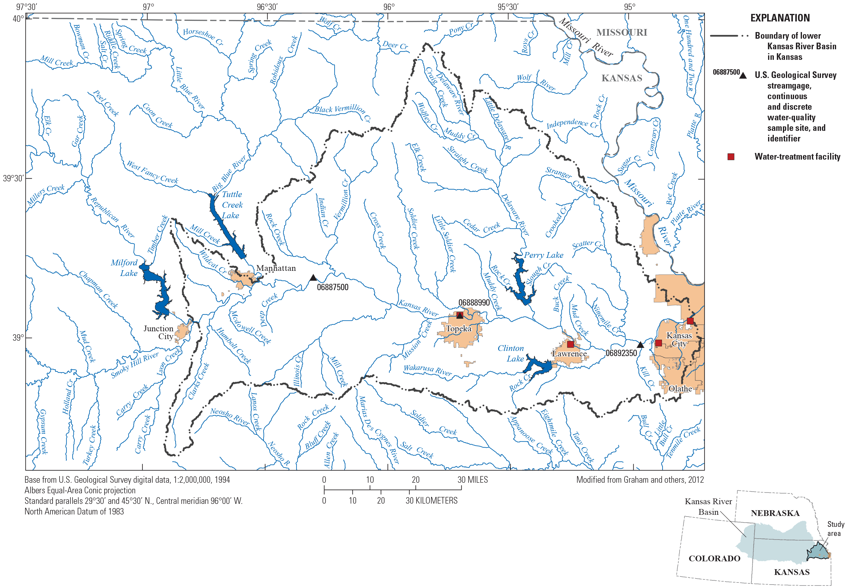
Location of the Kansas River at Wamego, Kansas; Kansas River above Topeka Weir at Topeka, Kans.; and Kansas River at De Soto, Kans., streamgages and discrete water-quality sampling sites in the lower Kansas River Basin (U.S. Geological Survey stations 06887500, 06888990, and 06892350, respectively).
Linear regression models that continuously compute water-quality constituent concentrations or densities were developed for the Topeka site, which is intermediately between the Wamego (rural, upstream) and De Soto (urban, downstream) monitoring sites (fig. 1). The Topeka site is on the southern bank of the Kansas River in Topeka and is about 40 river miles downstream from the Wamego site, about 58 river miles upstream from the De Soto site, and upstream from water-treatment facilities in Lawrence, Olathe, and Kansas City, Kans. (fig. 1). Public recreation, including kayaking, boating, and fishing, is common downstream from the Topeka site using a nearby access ramp.
Methods
The USGS collected continuous and discrete water-quality data at the Topeka site over the range of observed streamflows during November 2018 through June 2021 (fig. 2). These data were used to develop linear regression models at the Topeka site for total dissolved solids, major ions, hardness as calcium carbonate, nutrients (nitrogen and phosphorus species), chlorophyll a, total suspended solids, suspended sediment, and E. coli bacteria.
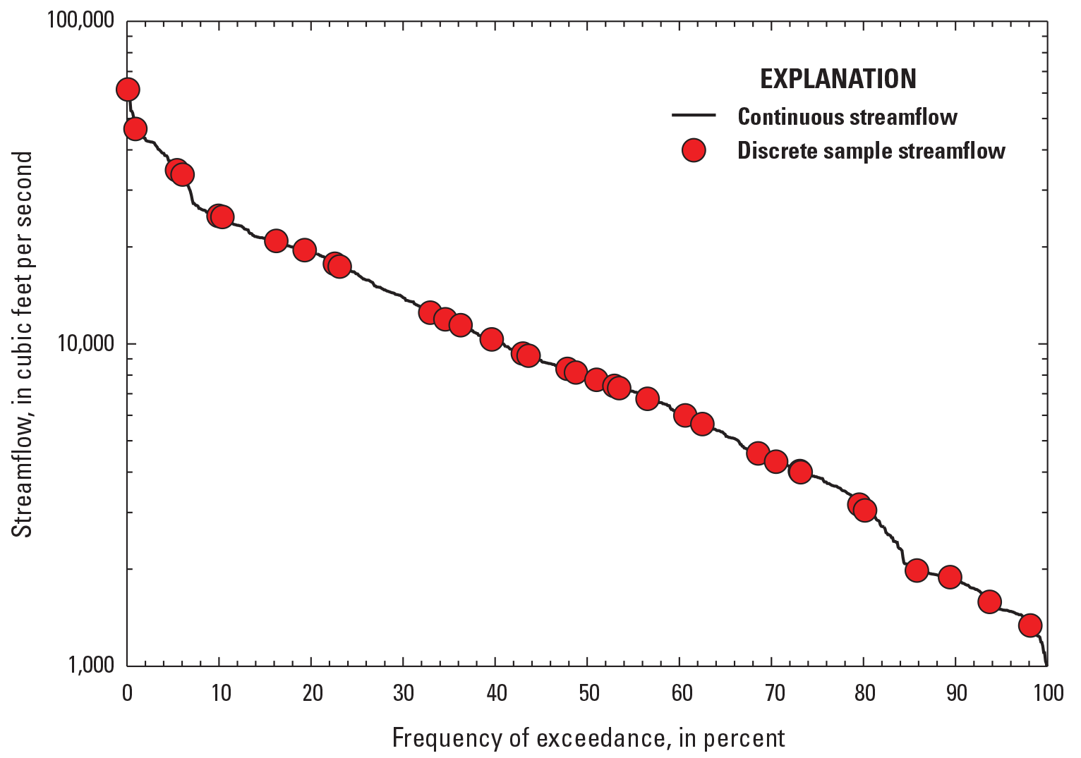
Streamflow duration curve and discrete water-quality samples at the Kansas River above Topeka Weir at Topeka, Kansas, streamgage (U.S. Geological Survey station 06888990) during November 2018 through June 2021. Data from U.S. Geological Survey, 2022.
Continuous Streamflow and Water-Quality Monitoring
The USGS began collecting continuous (15-minute interval) streamflow data at the Topeka site during November 2015 (U.S. Geological Survey, 2022) using standard USGS methods (Sauer and Turnipseed, 2010; Turnipseed and Sauer, 2010). These data are available in near-real time (hourly) from the USGS National Water Information System database at https://doi.org/10.5066/F7P55KJN (U.S. Geological Survey, 2022) by using station number 06888990.
The USGS began collecting continuous (15-minute interval) water-quality data at the Topeka site in November 2018. During November 2018 through June 2021, a YSI EXO2 water-quality monitor (YSI, Inc., 2017) was deployed by suspension from a building structure about 1 to 3 feet below the water surface on the southern bank of the Kansas River (fig. 3). Limited access and safety concerns prevented the use of bridge deployment at the centroid of flow (optimal deployment method used at the Wamego and De Soto sites; Williams [2021]). The water-quality monitor was equipped with water temperature, specific conductance, pH, dissolved oxygen, turbidity, and chlorophyll and phycocyanin fluorescence sensors. The water-quality monitor was operated and maintained using standard USGS methods (Wagner and others, 2006; Bennett and others, 2014). All continuous water-quality data are available in near-real time (hourly) from the USGS National Water Information System database at https://doi.org/10.5066/F7P55KJN (U.S. Geological Survey, 2022) by using station number 06888990.
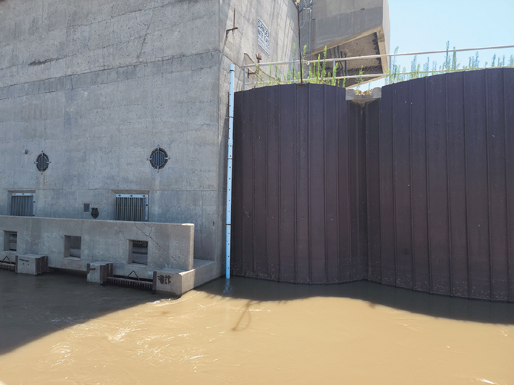
Continuous water-quality monitor deployment at the Kansas River above Topeka Weir at Topeka, Kansas, streamgage (U.S. Geological Survey station 06888990) during November 2018 through June 2021. Photograph by Joey Filby, City of Topeka.
Discrete Water-Quality Sampling
Water-quality samples were collected at the Topeka site on a biweekly to monthly basis during November 2018 through June 2020, on a monthly to bimonthly basis during July 2020 through June 2021, and during selected reservoir release and runoff events. Using this fixed-schedule sampling approach, water-quality samples were collected over the range of study period streamflows (fig. 2). Initially, during November 18, 2018, through February 5, 2019, three water-quality samples were collected 0.2 mi downstream from the continuous water-quality monitor location using depth- and width-integrated sampling techniques (U.S. Geological Survey, 2006) from a watercraft. This location was selected for safety reasons because of proximity of an upstream low-head dam (0.1 mi downstream from the continuous water-quality monitor location). Remaining samples were collected from the continuous water-quality monitor location because of greater accessibility throughout the study period streamflow range. Therefore, during February 19, 2019, through June 2021, all samples, excluding E. coli bacteria, were collected from the water-quality monitor location using a US DH–95 or US D–95 sampler (Edwards and Glysson, 1999) with depth-integrated sampling techniques (U.S. Geological Survey, 2006). Samples of E. coli bacteria were collected from the same location using a sterile, autoclaved bottle in a weighted basket. The water-quality monitor location provided the greatest safety and allowed for consistent sampling methodology and location regardless of streamflow conditions. All water-quality samples were analyzed for total dissolved solids, major ions, hardness as calcium carbonate, total nitrogen (particulate plus dissolved nitrogen), total Kjeldahl nitrogen (TKN; total concentration of organic nitrogen and ammonia), total phosphorus, chlorophyll a, total suspended solids, suspended sediment, and E. coli bacteria.
Total dissolved solids, major ions, hardness as calcium carbonate, nutrients (nitrogen and phosphorus species), and total suspended solids were analyzed by the USGS National Water Quality Laboratory in Lakewood, Colorado, using the methods documented by Fishman and Friedman (1989). Chlorophyll a was analyzed by the USGS National Water Quality Laboratory in Lakewood, Colo., using U.S. Environmental Protection Agency Method 445.0 (Arar and Collins, 1997). Suspended-sediment concentration was analyzed at the USGS Iowa Sediment Laboratory in Iowa City, Iowa, following methods documented by Guy (1969). Samples of E. coli bacteria were analyzed by the USGS Kansas Water Science Center following the methods documented by Myers and others (2014). All of these data are available from the USGS National Water Information System database at https://doi.org/10.5066/F7P55KJN (U.S. Geological Survey, 2022) by using station number 06888990.
Phytoplankton community composition and abundance, microcystin (a cyanotoxin), and geosmin and 2-methylisoborneol (taste-and-odor compounds) samples also were collected during each water-quality sampling. However, additional data collected during cyanobacteria, microcystin, and taste-and-odor events are necessary to obtain representative model-calibration datasets for model development at the Topeka site. Water-quality sampling and analytical methodology for these constituents are described in greater detail by Foster and Graham (2016) and Graham and others (2018).
Quality Assurance and Quality Control of Continuous and Discrete Water-Quality Data
All continuous and discrete water-quality data collected during November 2018 through June 2021 were reviewed and approved quarterly, following USGS guidance (U.S. Geological Survey, 2016, 2017). Continuous water-quality data occasionally were corrected or deleted because of fouling, sensor calibration drift (Wagner and others, 2006; Bennett and others, 2014), equipment malfunction, or temporary removal of the water-quality monitor to avoid loss or damage during below-freezing surface-water temperatures. During November 2018 through June 2021, about 3 percent of the water-temperature, pH, dissolved oxygen, and phycocyanin fluorescence records and about 4 percent of the specific conductance, turbidity, and chlorophyll fluorescence records at the Topeka site were missing or deleted because of excessive fouling.
Quality-control (QC) samples were collected for about 10 percent of all discrete water-quality samples. Concurrent replicate QC samples were collected to characterize variability in sample results that could potentially be introduced by sample-collection methods, sample processing techniques, and analytical method (Rasmussen and others, 2014; Mueller and others, 2015). Relative percentage difference (RPD) was used to quantify differences in noncensored (data reported as greater than or equal to the laboratory minimum reporting limit [MRL]) constituent concentrations or densities among concurrent replicate pairs and was calculated by dividing the absolute difference of a replicate pair of samples by their mean value and multiplying by 100 (Zar, 1999). Concurrent replicate RPDs met QC objectives if a constituent’s median RPD was less than or equal to 5 percent for total dissolved solids, major ions, and hardness as calcium carbonate; less than or equal to 10 percent for nutrients (nitrogen and phosphorus species), chlorophyll a, total suspended solids, and suspended-sediment concentration; and less than or equal to 30 percent for E. coli bacteria (Williams, 2021). Three concurrent replicate pairs were collected from the Topeka site during November 2018 through June 2021. QC objectives were met for concurrent replicate pairs for all constituents used for model development documented in this report. Median RPDs among concurrent replicate pairs for total dissolved solids, major ions, and hardness as calcium carbonate were less than 1 percent. Nutrient (nitrogen and phosphorus species) and chlorophyll a median concurrent replicate RPDs were less than 4 percent. Median concurrent replicate RPDs were less than 9 percent for total suspended solids and suspended-sediment concentration. The median RPD among E. coli bacteria concurrent replicates was 20 percent. Variability among E. coli bacteria concurrent replicate densities can increase if samples are insufficiently mixed during sample processing (Myers and others, 2014).
Three field blank samples were collected from the Topeka site during November 2018 through June 2021 to characterize bias caused by sampling procedures and analytical methods (Mueller and others, 2015). QC objectives were met if field blank sample concentrations were less than or equal to the associated MRL. Field blank sample concentrations were less than or equal to MRLs with the exception of one sample analyte. Chloride was the single constituent that had at least one detection (0.03 milligram per liter [mg/L]) greater than the MRL (0.02 mg/L) in all blank samples collected during the study period. Equipment- and procedure-blank samples were collected for all E. coli bacteria samples during November 2018 through June 2021. No E. coli bacteria detections were in any equipment- or procedure-blank samples during the study period.
Concomitant field and in situ water-quality monitor (YSI EXO2) physiochemical properties were measured during discrete sampling events to compare sample-collection methods (depth- and width-integrated [collection method used during November 18, 2018, through February 5, 2019] and depth-integrated [collection method used during February 19, 2019, through June 2021]). Cross-sectional profile water-quality physiochemical properties were measured about 1 foot below the water surface alongside the depth- and width-integrated discretely collected samples; these samples coincided with the 84th, 81st, and 52d percentiles of daily mean study period streamflows. Two sets of vertical-profile cross-sectional water-quality physiochemical properties were measured at several depths at each cross-section location; these two vertical-profile cross-sectional measurements coincided with the 19th and 69th percentiles of daily mean study period streamflows. The Topeka site’s stream conditions were arbitrarily considered to be well mixed if field-measured profile and in situ measurement statistics (water temperature, specific conductance, and dissolved oxygen means and pH medians) were within 5 percent. RPDs among concomitant cross-sectional and in situ continuous water-quality monitor statistics were calculated to determine if the initial depth- and width-integrated samples were comparable to the depth-integrated samples collected at the in situ continuous water-quality monitor location. RPDs among concomitant cross-sectional profile and in situ continuous water-quality monitor measurement statistics were less than 4 percent. RPDs among concomitant vertical-profile cross-sectional and in situ continuous water-quality monitor statistics were equal to or less than 3 percent. This information indicated that the Kansas River at the Topeka site likely was generally well mixed; therefore, all water-quality samples, regardless of sample-collection technique, were considered during model development.
Development of Regression Models
Models that related continuous in situ water-quality sensor measurements, streamflow, and seasonal components to discrete sample water-quality constituent concentrations or densities using linear regression analysis and data collected during November 2018 through June 2021 were developed. All regression models were developed using R programming language, version 4.2.0 (R Core Team, 2022). Models were developed using ordinary least squares estimation for constituents with model-calibration datasets containing no left-censored data (data reported as less than the laboratory MRL). Ordinary least squares estimation was used to develop models that compute continuous concentrations or densities of total dissolved solids, calcium, magnesium, sodium, sulfate, chloride, hardness as calcium carbonate, total nitrogen (particulate plus dissolved nitrogen), TKN, total phosphorus, chlorophyll a, suspended sediment, and E. coli bacteria. These constituents were selected for model development based on evaluation of model-diagnostic statistics, relevance to water-treatment managers, association with State water-quality criteria or impairments, previously published Kansas River models (Rasmussen and others, 2005; Foster and Graham, 2016; Williams, 2021), and overall dataset suitability for model development. If censored data were present in a constituent’s model-calibration dataset, then Tobit regression estimation was used to develop models using the absolute maximum likelihood estimation procedure (Hald, 1949; Cohen, 1950; Tobin, 1958; Helsel and others, 2020). Absolute maximum likelihood estimation was used to develop the model that computes continuous concentrations of total suspended solids. Percentages of censored data and the model estimation method for each water-quality constituent are reported in table 1 and appendixes 1–14.
Table 1.
Linear regression models and summary statistics for computations of continuous water-quality constituent concentrations or densities for the Kansas River above Topeka Weir at Topeka, Kansas, streamgage (U.S. Geological Survey station 06888990) using data collected during November 2018 through June 2021.[R2, coefficient of determination; MSE, mean square error; RMSE, root mean square error; RSE, residual standard error; MSPE, model standard percentage error; n, number of discrete samples used in model development dataset; mg/L, milligram per liter; SC, continuously measured specific conductance in microsiemens per centimeter at 25 degrees Celsius; OLS, ordinary least squares; app., appendix; --, not applicable; log, logarithm with base 10; CaCO3, calcium carbonate; TBY, turbidity in formazin nephelometric units; AMLE, absolute maximum likelihood estimation; μg/L, microgram per liter; fCHL, chlorophyll fluorescence at wavelength of 650 to 700 nanometers in relative fluorescence units; <, less than; colonies/100 mL, colonies per 100 milliliters]
| Regression model | Regression estimation method | Model archival summary | Adjusted R2 | aPseudo-R2 | MSE | RMSE | Estimated RSE (unbiased) | Mean MSPE | Bias correction factor (Duan, 1983) | Discrete data used in model development dataset | ||||
|---|---|---|---|---|---|---|---|---|---|---|---|---|---|---|
| n | Percentage of censored data | Range of values in variable measurements | Mean | Median | ||||||||||
| Total dissolved solids (TDS), mg/L | ||||||||||||||
| TDS=0.584(SC)+39.3 | OLS | App. 1 | 0.974 | -- | 1,000 | 31.7 | 31.7 | 6.16 | -- | 34 | 0 | TDS: 202–839 | 514 | 502 |
| SC: 188–1,420 | 814 | 778 | ||||||||||||
| Calcium (Ca), dissolved, mg/L | ||||||||||||||
| log(Ca)=0.739log(SC)−0.234 | OLS | App. 2 | 0.938 | -- | 0.00159 | 0.0399 | 0.0399 | 9.21 | 1.00 | 34 | 0 | Ca: 31.7–120 | 81.7 | 85.3 |
| SC: 188–1,420 | 814 | 778 | ||||||||||||
| Magnesium (Mg), dissolved, mg/L | ||||||||||||||
| log(Mg)=0.893log(SC)−1.35 | OLS | App. 3 | 0.954 | -- | 0.00169 | 0.0411 | 0.0411 | 9.48 | 1.00 | 34 | 0 | Mg: 4.96–27.7 | 17.6 | 19.0 |
| SC: 188–1,420 | 814 | 778 | ||||||||||||
| Sodium (Na), dissolved, mg/L | ||||||||||||||
| log(Na)=1.63log(SC)−3.00 | OLS | App. 4 | 0.981 | -- | 0.00229 | 0.0479 | 0.0479 | 11.1 | 1.01 | 34 | 0 | Na: 3.75–158 | 62.3 | 52.9 |
| SC: 188–1,420 | 814 | 778 | ||||||||||||
| Sulfate (SO4), dissolved, mg/L | ||||||||||||||
| log(SO4)=1.38log(SC)−1.97 | OLS | App. 5 | 0.932 | -- | 0.00613 | 0.0783 | 0.0783 | 18.1 | 1.01 | 34 | 0 | SO4: 9.22–196 | 116 | 126 |
| SC: 188–1,420 | 814 | 778 | ||||||||||||
| Chloride (Cl), dissolved, mg/L | ||||||||||||||
| log(Cl)=1.83log(SC)−3.48 | OLS | App. 6 | 0.967 | -- | 0.00498 | 0.0706 | 0.0706 | 16.3 | 1.01 | 34 | 0 | Cl: 3.01–228 | 79.0 | 62.8 |
| SC: 188–1,420 | 814 | 778 | ||||||||||||
| Hardness (CaCO3), mg/L | ||||||||||||||
| log(CaCO3)=0.771log(SC)+0.201 | OLS | App. 7 | 0.947 | -- | 0.00145 | 0.0381 | 0.0381 | 8.78 | 1.00 | 34 | 0 | CaCO3: 99.8–412 | 276 | 289 |
| SC: 188–1,420 | 814 | 778 | ||||||||||||
| Total nitrogen (TN), total particulate nitrogen plus dissolved nitrogen, mg/L | ||||||||||||||
| log(TN)=0.373log(TBY)−0.387 | OLS | App. 8 | 0.743 | -- | 0.0182 | 0.135 | 0.135 | 31.7 | 1.05 | 34 | 0 | TN: 0.788–8.03 | 2.62 | 1.94 |
| TBY: 8.23–1,240 | 230 | 60.6 | ||||||||||||
| Total Kjeldahl nitrogen (TKN), mg/L; total ammonia plus organic nitrogen, mg/L | ||||||||||||||
| log(TKN)=0.507log(TBY)−0.902 | OLS | App. 9 | 0.922 | -- | 0.00837 | 0.0915 | 0.0915 | 21.2 | 1.02 | 34 | 0 | TKN: 0.440–5.80 | 1.65 | 0.875 |
| TBY: 8.23–1,240 | 230 | 60.6 | ||||||||||||
| Total phosphorus (TP), mg/L | ||||||||||||||
| log(TP)=0.566log(TBY)−1.43 | OLS | App. 10 | 0.914 | -- | 0.0117 | 0.108 | 0.108 | 25.2 | 1.03 | 34 | 0 | TP: 0.140–2.45 | 0.668 | 0.390 |
| TBY: 8.23–1,240 | 230 | 60.6 | ||||||||||||
| Chlorophyll a, (Chla), μg/L | ||||||||||||||
| log(Chla)=1.26log(fCHL)+0.687 | OLS | App. 11 | 0.809 | -- | 0.0392 | 0.198 | 0.198 | 47.1 | 1.1 | 34 | 0 | Chla: 1.40–59.9 | 19.2 | 13.8 |
| fCHL: 0.697–7.96 | 2.78 | 1.75 | ||||||||||||
| Total suspended solids, (TSS), mg/L | ||||||||||||||
| log(TSS)=1.06log(TBY)+0.205 | AMLE | App. 12 | -- | 0.943 | -- | -- | 0.165 | -- | 1.06 | 34 | 5.90 | TSS: <15.0–3,480 | 526 | 136 |
| TBY: 8.23–1,240 | 230 | 60.6 | ||||||||||||
| Suspended-sediment concentration (SSC), mg/L | ||||||||||||||
| log(SSC)=1.07log(TBY)+0.29 | OLS | App. 13 | 0.989 | -- | 0.0051 | 0.0712 | 0.0712 | 16.5 | 1.01 | 33 | 0 | SSC: 18–3,710 | 735 | 161 |
| TBY: 8.23–1,240 | 236 | 61.0 | ||||||||||||
| Escherichia coli bacteria (ECB), colonies/100 mL | ||||||||||||||
| log(ECB)=1.69log(TBY)−1.04 | OLS | App. 14 | 0.791 | -- | 0.289 | 0.538 | 0.538 | 158 | 1.85 | 34 | 0 | ECB: 6.00–41,000 | 4,510 | 64.0 |
| TBY: 8.23–1,240 | 230 | 60.6 | ||||||||||||
Pseudo-R2 is computed using the McKelvey-Zavoina method (McKelvey and Zavoina, 1975). For uncensored data, pseudo-R2 is equal to the R2 value for ordinary least squares.
Chlorophyll a and E. coli bacteria sample data included some results qualified as “estimated” in accordance with standard laboratory quality-assurance procedures. Estimated results were investigated as potential outliers by confirming correct database entry, evaluating laboratory analytical performance, and reviewing all field notes associated with the samples in question (Rasmussen and others, 2009). Estimated results within the chlorophyll a and E. coli bacteria model-calibration datasets are identified in appendixes 11 and 14, respectively; were not determined to have errors associated with sample collection, processing, or analysis; and were therefore considered valid.
Potential explanatory variables that were considered during linear regression model development were continuous streamflow, water temperature, specific conductance, dissolved oxygen, turbidity, chlorophyll and phycocyanin fluorescence, and seasonal components (sine and cosine variables). Potential explanatory variables were evaluated individually and in combination and were interpolated by discrete water-quality sample time within the 15-minute continuous record. Explanatory variable data were not interpolated by sample time if the sample time coincided with a gap in the continuous record (because of excessive fouling, equipment malfunction, or equipment removal) that exceeded 2 hours (Williams, 2021). If gaps in the continuous record exceeded 2 hours and prevented interpolation based on discrete water-quality sample time, then data collected using water-quality monitors during discrete sample collection were used for inclusion in the model-calibration dataset.
Preliminary linear regression models were evaluated based on range and distribution of continuous and discrete model-calibration data, patterns in residual plots, and the following model diagnostic statistics: adjusted coefficient of determination (R2), pseudo-R2 (computed for Tobit regression models only; McKelvey and Zavoina, 1975), Mallows’ Cp (Mallows, 1973), root mean square error (RMSE), and prediction error sum of squares (PRESS; Rasmussen and others, 2009; Helsel and others, 2020). The best linear regression model was selected for each response variable (total dissolved solids, calcium, magnesium, sodium, sulfate, chloride, hardness as calcium carbonate, total nitrogen [particulate plus dissolved nitrogen], TKN, total phosphorus, chlorophyll a, total suspended solids, suspended sediment, and E. coli bacteria) when variance explained by the model (adjusted R2 or pseudo-R2) was maximized and greater than or equal to 0.60, model precision was high and model bias was low (Mallows’ Cp), uncertainty in model computations was minimized (RMSE and PRESS), and heteroscedasticity (irregular scatter) was minimal in residual plots (Rasmussen and others, 2009; Helsel and others, 2020). Potential explanatory variables were not included in the final selected regression model if they had a probability greater than 0.05. Model simplicity and previously published explanatory variables at other Kansas River sites (Rasmussen and others, 2005; Foster and Graham 2016; Williams, 2021) also were considered during the model selection process.
Logarithmic transformations (logarithm with base 10 [log] transformations) of the response and explanatory variables were used during model development if heteroscedasticity was apparent in plots of response variable residuals compared to model computed values (shown in appendixes 1–14). If log transformations were used in the final selected model, a bias correction factor was computed and used for the retransformation of log-transformed computations back into their original units (Duan, 1983) to reduce inherent negative bias introduced by log transformations (Helsel and others, 2020).
Multiple explanatory variables for a given linear regression model were considered if the additional variable increased the variance (as indicated by adjusted R2 or pseudo-R2) explained by the model by at least 5 percent, decreased Mallows’ Cp, minimized RMSE and PRESS, and minimized heteroscedasticity in residual plots. Additionally, multiple explanatory variables were considered for inclusion in the final selected model if their variance inflation factors (Marquardt, 1970) were less than 4, indicating minimal multicollinearity (O’Brien, 2007; Vatcheva and others, 2016; Helsel and others, 2020).
Potential outliers initially were identified by viewing bivariate plots of the model-calibration data for each set of response and explanatory variables (Rasmussen and others, 2009). Studentized residuals from preliminary models were inspected for values greater than three or less than negative three (Pardoe, 2020). Values outside of that range were considered potential outliers and were investigated. Additionally, computations of leverage, Cook’s distance, and difference in fits statistics were used to estimate potential outlier effect on the final selected regression model (Cook, 1977; Helsel and others, 2020). Outliers were investigated for potential removal from the model-calibration dataset by confirming correct database entry, evaluating laboratory analytical performance, and reviewing field notes associated with the sample in question (Rasmussen and others, 2009). Outlier identification and justification for removal are included, when applicable, in appendixes 1–14. Model development methodology is described in additional detail in appendixes 1–14.
Developed Regression Models
Linear regression models that compute continuous water-quality constituent concentrations or densities of total dissolved solids, calcium, magnesium, sodium, sulfate, chloride, hardness as calcium carbonate, total nitrogen (particulate plus dissolved nitrogen), TKN, total phosphorus, chlorophyll a, total suspended solids, suspended sediment, and E. coli bacteria were developed. A single model was selected for each constituent. Each model form, model diagnostic statistics, and data summary statistics are listed in table 1. Model archival summaries that document model development information, statistical output (R Core Team, 2022), and model-calibration datasets are provided in appendixes 1–14.
Total Dissolved Solids, Major Ions, and Hardness
Specific conductance was the single explanatory variable used to model for total dissolved solids, calcium, magnesium, sodium, sulfate, chloride, and hardness as calcium carbonate at the Topeka site (table 1; appendixes 1–7). Specific conductance, a measure of the surface water’s ability to conduct an electrical current, is positively correlated with total dissolved solids and other charged ionic species (Hem, 1985) and explained about 93–98 percent of the variance (as indicated by adjusted R2) in total dissolved solids, major ions, and hardness as calcium carbonate concentrations (table 1; appendixes 1–7). Specific conductance was also the single explanatory variable used to model for these constituents in previously published models at the Wamego and De Soto sites (Rasmussen and others, 2005; Foster and Graham, 2016; Williams, 2021).
Total Nitrogen, Total Kjeldahl Nitrogen, Total Phosphorus, and Chlorophyll a
Turbidity was the single explanatory variable used to model for total nitrogen, TKN, and total phosphorus at the Topeka site (table 1; appendixes 8–10). Turbidity, a measure of surface-water clarity caused by the presence of suspended and dissolved material, typically increases during precipitation runoff events. Nutrients, as well as other contaminants, tend to physically bind to suspended and dissolved material in the Kansas River (Rasmussen and others, 2005; Graham and others, 2018). Turbidity explained about 74, 92, and 91 percent of variability in total nitrogen, TKN, and total phosphorus concentrations, respectively (table 1). The TKN model may overestimate computed TKN concentrations in the low (0.0 to 0.70 mg/L) and high (3.11 to 4.73 mg/L) ranges and underestimate computed TKN concentrations in the middle range (0.71 to 3.10 mg/L) because of larger scatter observed in plots of residual and regression computed TKN and residual TKN and turbidity (appendix 9). Additional TKN model-calibration data may improve this limitation in the future. Turbidity also was selected as an explanatory variable for nutrient (nitrogen and phosphorus species) models published by Rasmussen and others (2005), Foster and Graham (2016), and Williams (2021) at the Wamego and De Soto sites.
Chlorophyll fluorescence was the single explanatory variable used to model for chlorophyll a at the Topeka site (table 1; appendix 11). Although an unknown level of uncertainty is inherent to fluorescence sensors (because of nonphotochemical quenching, matrix effects, and variable fluorescence responses of differing plankton communities [Foster and others, 2022]), chlorophyll fluorescence makes physical and statistical sense as an explanatory variable for chlorophyll a because chlorophyll a pigments fluoresce when irradiated by certain wavelengths of light emitted from the chlorophyll fluorescence sensor. Chlorophyll fluorescence explained about 81 percent of the variability in chlorophyll a concentration. The chlorophyll a model may overestimate computed chlorophyll a concentration in the upper range based on irregular scatter in the plot of observed and regression computed chlorophyll a (appendix 11). Additional chlorophyll a model-calibration data may improve this limitation in the future. Chlorophyll fluorescence was also the single explanatory variable used to model for chlorophyll a concentration in the models previously published by Williams (2021) at the Wamego and De Soto sites.
Total Suspended Solids and Suspended Sediment
Turbidity was the single explanatory variable used to model for total suspended solids and suspended sediment at the Topeka site (table 1; appendixes 12 and 13). Turbidity was positively correlated with total suspended solids and suspended sediment and explained about 94 and 99 percent of the variance in these constituents, respectively. Turbidity was also the single explanatory variable used to model for these constituents in the models previously published by Rasmussen and others (2005), Foster and Graham (2016; did not publish models for total suspended solids), and Williams (2021) at the Wamego and De Soto sites.
Escherichia coli Bacteria
Turbidity was the single explanatory variable used to model for E. coli bacteria at the Topeka site (table 1; appendix 14), likely because E. coli tend to physically bind to suspended material. Turbidity explained about 79 percent of the variance in E. coli density and was also the single explanatory variable used to model for E. coli models previously published by Rasmussen and others (2005), Foster and Graham (2016; published E. coli model for De Soto site only), and Williams (2021) at the Wamego and De Soto sites.
Summary
Water suppliers rely on the Kansas River and its alluvial aquifer to supply drinking water to more than 950,000 people throughout northeastern Kansas. They use numerous physiochemical processes to treat and remove contaminants from source water before public distribution. An early-notification system of changing water-quality conditions near water-supply intakes allows water suppliers to proactively make decisions that affect water treatment. The U.S. Geological Survey (USGS), in cooperation with the Kansas Water Office (funded in part through the Kansas Water Plan), the Kansas Department of Health and Environment, The Nature Conservancy, the City of Lawrence, the City of Manhattan, the City of Olathe, the City of Topeka, WaterOne, and Evergy, established a new continuous and discrete water-quality monitoring site at the Kansas River above Topeka Weir at Topeka, Kansas (USGS site 06888990; hereafter referred to as the “Topeka site”), in November 2018 to expand the Kansas River water-quality monitoring network by adding an intermediate location between the existing monitoring sites at Wamego (upstream) and De Soto (downstream), Kans. The continuous and discrete water-quality data were collected by the USGS at the Topeka site over the range of observed streamflow conditions during November 2018 through June 2021 and were used to develop new linear regression models and expand the early-notification system of changing water-quality conditions that may affect water treatment. Continuous water-quality data collected at the site were water temperature, specific conductance, pH, dissolved oxygen, turbidity, and chlorophyll and phycocyanin fluorescence. All discrete water-quality samples were analyzed for total dissolved solids, major ions, hardness as calcium carbonate, nutrients (nitrogen and phosphorus species), chlorophyll a, total suspended solids, suspended sediment, and Escherichia coli bacteria. Models that relate the continuous water-quality sensor measurements to discrete sample water-quality constituent concentrations or densities were developed for total dissolved solids, calcium, magnesium, sodium, sulfate, chloride, hardness as calcium carbonate, total nitrogen [particulate plus dissolved nitrogen], total Kjeldahl nitrogen, total phosphorus, chlorophyll a, total suspended solids, suspended sediment, and Escherichia coli bacteria. Evaluating model performance on an ongoing basis will be necessary to continue to provide model computations in the future. Additional model-calibration data collected during conditions outside of those observed during the study period may improve future model performance.
The models documented in this report provide real-time computations of water-quality constituent concentrations or densities that are not easily measured in real time. Model computations are useful to the public for cultural and recreational purposes and can be used to characterize water-quality conditions that may affect drinking-water treatment at the Topeka site, compare to previously published model-computed concentrations or densities at the Wamego and De Soto sites, compare conditions with Federal and State water-quality criteria, and evaluate changes in water-quality conditions in the Kansas River through time.
References Cited
Bennett, T.J., Graham, J.L., Foster, G.M., Stone, M.L., Juracek, K.E., Rasmussen, T.J., and Putnam, J.E., 2014, U.S. Geological Survey quality-assurance plan for continuous water-quality monitoring in Kansas, 2014: U.S. Geological Survey Open-File Report 2014–1151, 34 p. plus appendixes, accessed April 2022 at https://doi.org/10.3133/ofr20141151.
Cohen, A.C., Jr., 1950, Estimating the mean and variance of normal populations from singly truncated and doubly truncated samples: Annals of Mathematical Statistics, v. 21, no. 4, p. 557–569, accessed April 2022 at https://doi.org/10.1214/aoms/1177729751.
Cook, R.D., 1977, Detection of influential observations in linear regression: Technometrics, v. 19, no. 1, p. 15–18. [Also available at https://www.jstor.org/stable/1268249.]
Duan, N., 1983, Smearing estimate—A nonparametric retransformation method: Journal of the American Statistical Association, v. 78, no. 383, p. 605–610. [Also available at https://doi.org/10.1080/01621459.1983.10478017.]
Edwards, T.K., and Glysson, D.G., 1999, Field methods for measurement of fluvial sediment: U.S. Geological Survey Techniques of Water-Resources Investigations, book 3, chap. C2, 89 p. [Also available at https://doi.org/10.3133/twri03C2.]
Fishman, M.J., and Friedman, L.C., 1989, Methods for determination of inorganic substances in water and fluvial sediments (3d ed.): U.S. Geological Survey Techniques of Water-Resources Investigations, book 5, chap. A1, 545 p. [Also available at https://doi.org/10.3133/twri05A1.]
Foster, G.M., and Graham, J.L., 2016, Logistic and linear regression model documentation for statistical relations between continuous real-time and discrete water-quality constituents in the Kansas River, Kansas, July 2012 through June 2015: U.S. Geological Survey Open-File Report 2016–1040, 27 p., accessed April 2022 at https://doi.org/10.3133/ofr20161040.
Foster, G.M., Graham, J.L., Bergamaschi, B.A., Carpenter, K.D., Downing, B.D., Pellerin, B.A., Rounds, S.A., and Saraceno, J.F., 2022, Field techniques for the determination of algal pigment fluorescence in environmental waters—Principles and guidelines for instrument and sensor selection, operation, quality assurance, and data reporting: U.S. Geological Survey Techniques and Methods, book 1, chap. D10, 34 p. [Also available at https://doi.org/10.3133/tm1D10.]
Graham, J.L., Foster, G.M., Williams, T.J., Mahoney, M.D., May, M.R., and Loftin, K.A., 2018, Water-quality conditions with an emphasis on cyanobacteria and associated toxins and taste-and-odor compounds in the Kansas River, Kansas, July 2012 through September 2016: U.S. Geological Survey Scientific Investigations Report 2018–5089, 55 p. [Also available at https://doi.org/10.3133/sir20185089.]
Graham, J.L., Ziegler, A.C., Loving, B.L., and Loftin, K.A., 2012, Fate and transport of cyanobacteria and associated toxins and taste-and-odor compounds from upstream reservoir releases in the Kansas River, Kansas, September and October 2011: U.S. Geological Survey Scientific Investigations Report 2012–5129, 65 p. [Also available at https://doi.org/10.3133/sir20125129.]
Guy, H.P., 1969, Laboratory theory and methods for sediment analysis: U.S. Geological Survey Techniques of Water-Resources Investigations, book 5, chap. C1, 58 p. [Also available at https://doi.org/10.3133/twri05C1.]
Hald, A., 1949, Maximum likelihood estimation of the parameters of a normal distribution which is truncated at a known point: Scandinavian Actuarial Journal, v. 1949, no. 1, p. 119–134. [Also available at https://doi.org/10.1080/03461238.1949.10419767.]
Helsel, D.R., Hirsch, R.M., Ryberg, K.R., Archfield, S.A., and Gilroy, E.J., 2020, Statistical methods in water resources: U.S. Geological Survey Techniques and Methods, book 4, chap. A3, 458 p. [Also available at https://doi.org/10.3133/tm4A3.] [Supersedes USGS Techniques of Water-Resources Investigations, book 4, chap. A3, version 1.1.]
Hem, J.D., 1985, Study and interpretation of the chemical characteristics of natural water (3d ed.): U.S. Geological Survey Water-Supply Paper 2254, 263 p, 4 pls. [Also available at https://doi.org/10.3133/wsp2254.]
Kansas Department of Health and Environment, 2011, Kansas-Lower Republican Basin [total maximum daily load]: Kansas Department of Health and Environment web page, accessed April 2022 at https://www.kdhe.ks.gov/1455/Kansas-Lower-Republican-River-Basin.
Mallows, C.L., 1973, Some comments on Cp: Technometrics, v. 15, no. 4, p. 661–675, accessed April 2022 at https://doi.org/10.1080/00401706.1973.10489103.
Marquardt, D.W., 1970, Generalized inverses, ridge regression, biased linear estimation, and nonlinear estimation: Technometrics, v. 12, no. 3, p. 591–612. [Also available at https://doi.org/10.2307/1267205.]
McKelvey, R.D., and Zavoina, W., 1975, A statistical model for the analysis of ordinal level dependent variables: The Journal of Mathematical Sociology, v. 4, no. 1, p. 103–120. [Also available at https://doi.org/10.1080/0022250X.1975.9989847.]
Mueller, D.K., Schertz, T.L., Martin, J.D., and Sandstrom, M.W., 2015, Design, analysis, and interpretation of field quality-control data for water-sampling projects: U.S. Geological Survey Techniques and Methods, book 4, chap. C4, 54 p., accessed April 2022 at https://doi.org/10.3133/tm4C4.
Myers, D.N., Stoeckel, D.M., Bushon, R.N., Francy, D.S., and Brady A.M.G., 2014, Chapter A7.1, Fecal indicator bacteria: U.S. Geological Survey Techniques of Water-Resources Investigations, book 9, chap. A7.1. [Also available at https://doi.org/10.3133/twri09A7.1.]
O’Brien, R.M., 2007, A caution regarding rules of thumb of variance inflation factors: Quality & Quantity, v. 41, no. 5, p. 673–690, accessed April 2022 at https://doi.org/10.1007/s11135-006-9018-6.
R Core Team, 2022, R—A language and environment for statistical computing: Vienna, Austria, R Foundation for Statistical Computing software release, accessed April 2022 at https://www.r-project.org/.
Rasmussen, P.P., Gray, J.R., Glysson, G.D., and Ziegler, A.C., 2009, Guidelines and procedures for computing time-series suspended-sediment concentrations and loads from in-stream turbidity sensor and streamflow data: U.S. Geological Survey Techniques and Methods, book 3, chap. C4, 53 p. [Also available at https://doi.org/10.3133/tm3C4.]
Rasmussen, T.J., Bennett, T.J., Stone, M.L., Foster, G.M., Graham, J.L., and Putnam, J.E., 2014, Quality-assurance and data-management plan for water-quality activities in the Kansas Water Science Center, 2014: U.S. Geological Survey Open-File Report 2014–1233, 41 p., accessed April 2022 at https://doi.org/10.3133/ofr20141233.
Rasmussen, T.J., Ziegler, A.C., and Rasmussen, P.P., 2005, Estimation of constituent concentrations, densities, loads, and yields in lower Kansas River, northeast Kansas, using regression models and continuous water-quality monitoring, January 2000 through December 2003: U.S. Geological Survey Scientific Investigations Report 2005–5165, 117 p. [Also available at https://doi.org/10.3133/sir20055165.]
Sauer, V.B., and Turnipseed, D.P., 2010, Stage measurement at gaging stations: U.S. Geological Survey Techniques and Methods, book 3, chap. A7, 45 p., accessed April 2022 at https://doi.org/10.3133/tm3A7.
Tobin, J., 1958, Estimation of relationships for limited dependent variables: Econometrica, v. 26, no. 1, p. 24–36. [Also available at https://doi.org/10.2307/1907382.]
Turnipseed, D.P., and Sauer, V.B., 2010, Discharge measurements at gaging stations: U.S. Geological Survey Techniques and Methods, book 3, chap. A8, 87 p., accessed April 2022 at https://doi.org/10.3133/tm3A8.
U.S. Army Corps of Engineers, 2017, Lakes in the Kansas City district: U.S. Army Corps of Engineers, web page, accessed April 2022 at https://www.nwk.usace.army.mil/Locations/.
U.S. Geological Survey, 2006, Collection of water samples (ver. 2.0, September 2006): U.S. Geological Survey Techniques of Water-Resources Investigations, book 9, chap. A4, 166 p. [Also available at https://doi.org/10.3133/twri09A4.]
U.S. Geological Survey, 2016, Policy and guidance for approval of surrogate regression models for computation of time series suspended-sediment concentrations and loads: U.S. Geological Survey Office of Water Quality Technical Memorandum no. 2016.10, accessed April 2022 at https://water.usgs.gov/admin/memo/QW/qw2016.10.pdf.
U.S. Geological Survey, 2017, Procedures for processing, approving, publishing, and auditing time-series records for water data: U.S. Geological Survey Office of Water Quality Technical Memorandum no. 2017.07, accessed April 2022 at https://water.usgs.gov/admin/memo/QW/qw2017.07.pdf.
U.S. Geological Survey, 2022, USGS water data for the Nation: U.S. Geological Survey National Water Information System database, accessed April 2022 at https://doi.org/10.5066/F7P55KJN.
Vatcheva, K.P., Lee, M., McCormick, J.B., and Rahbar, M.H., 2016, Multicollinearity in regression analyses conducted in epidemiologic studies: Epidemiology, v. 6, no. 2, 9 p., accessed April 2022 at https://doi.org/10.4172/2161-1165.1000227.
Wagner, R.J., Boulger, R.W., Jr., Oblinger, C.J., and Smith, B.A., 2006, Guidelines and standard procedures for continuous water-quality monitors—Station operation, record computation, and data reporting: U.S. Geological Survey Techniques and Methods, book 1, chap. D3, 51 p. plus 8 attachments. [Also available at https://doi.org/10.3133/tm1D3.] [Supersedes USGS Water-Resources Investigations Report 2000–4252.]
Williams, T.J., 2021, Linear regression model documentation and updates for computing water-quality constituent concentrations or densities using continuous real-time water-quality data for the Kansas River, Kansas, July 2012 through September 2019: U.S. Geological Survey Open-File Report 2021–1018, 18 p., accessed April 2022 at https://doi.org/10.3133/ofr20211018.
YSI, Inc., 2017, EXO user manual—Advanced water quality monitoring platform (rev. G): Yellow Springs, Ohio, YSI, Inc., 154 p., accessed April 2022 at https://www.ysi.com/file%20library/documents/manuals/exo-user-manual-web.pdf.
Appendixes 1. –14. Model Archival Summaries
-
Appendix 1. Model Archival Summary for Total Dissolved Solids Concentration at U.S. Geological Survey Site 06888990, Kansas River above Topeka Weir at Topeka, Kansas, during November 2018 through June 2021
-
Appendix 2. Model Archival Summary for Calcium Concentration at U.S. Geological Survey Site 06888990, Kansas River above Topeka Weir at Topeka, Kansas, during November 2018 through June 2021
-
Appendix 3. Model Archival Summary for Magnesium Concentration at U.S. Geological Survey Site 06888990, Kansas River above Topeka Weir at Topeka, Kansas, during November 2018 through June 2021
-
Appendix 4. Model Archival Summary for Sodium Concentration at U.S. Geological Survey Site 06888990, Kansas River above Topeka Weir at Topeka, Kansas, during November 2018 through June 2021
-
Appendix 5. Model Archival Summary for Sulfate Concentration at U.S. Geological Survey Site 06888990, Kansas River above Topeka Weir at Topeka, Kansas, during November 2018 through June 2021
-
Appendix 6. Model Archival Summary for Chloride Concentration at U.S. Geological Survey Site 06888990, Kansas River above Topeka Weir at Topeka, Kansas, during November 2018 through June 2021
-
Appendix 7. Model Archival Summary for Hardness Concentration at U.S. Geological Survey Site 06888990, Kansas River above Topeka Weir at Topeka, Kansas, during November 2018 through June 2021
-
Appendix 8. Model Archival Summary for Total Nitrogen Concentration at U.S. Geological Survey Site 06888990, Kansas River above Topeka Weir at Topeka, Kansas, during November 2018 through June 2021
-
Appendix 9. Model Archival Summary for Total Kjeldahl Nitrogen Concentration at U.S. Geological Survey Site 06888990, Kansas River above Topeka Weir at Topeka, Kansas, during November 2018 through June 2021
-
Appendix 10. Model Archival Summary for Total Phosphorus Concentration at U.S. Geological Survey Site 06888990, Kansas River above Topeka Weir at Topeka, Kansas, during November 2018 through June 2021
-
Appendix 11. Model Archival Summary for Chlorophyll a Concentration at U.S. Geological Survey Site 06888990, Kansas River above Topeka Weir at Topeka, Kansas, during November 2018 through June 2021
-
Appendix 12. Model Archival Summary for Total Suspended Solids Concentration at U.S. Geological Survey Site 06888990, Kansas River above Topeka Weir at Topeka, Kansas, during November 2018 through June 2021
-
Appendix 13. Model Archival Summary for Suspended-Sediment Concentration at U.S. Geological Survey Site 06888990, Kansas River above Topeka Weir at Topeka, Kansas, during December 2018 through June 2021
-
Appendix 14. Model Archival Summary for Escherichia coli Bacteria Concentration at U.S. Geological Survey Site 06888990, Kansas River above Topeka Weir at Topeka, Kansas, during November 2018 through June 2021
Conversion Factors
Supplemental Information
Specific conductance is given in microsiemens per centimeter at 25 degrees Celsius (µS/cm at 25 °C).
Concentrations of chemical constituents in water are given in either milligrams per liter (mg/L) or micrograms per liter (µg/L).
Densities of Escherichia coli bacteria are given in colony forming units per 100 milliliters (cfu/100 mL).
For more information about this publication, contact:
Director, USGS Kansas Water Science Center
1217 Biltmore Drive
Lawrence, KS 66049
785–842–9909
For additional information, visit: https://www.usgs.gov/centers/kswsc
Publishing support provided by the
Rolla Publishing Service Center
Suggested Citation
Williams, T.J., 2023, Linear regression model documentation for computing water-quality constituent concentrations or densities using continuous real-time water-quality data for the Kansas River above Topeka Weir at Topeka, Kansas, November 2018 through June 2021: U.S. Geological Survey Scientific Investigations Report 2022–5130, 14 p., https://doi.org/10.3133/sir20225130.
ISSN: 2328-0328 (online)
Study Area
| Publication type | Report |
|---|---|
| Publication Subtype | USGS Numbered Series |
| Title | Linear regression model documentation for computing water-quality constituent concentrations or densities using continuous real-time water-quality data for the Kansas River above Topeka Weir at Topeka, Kansas, November 2018 through June 2021 |
| Series title | Scientific Investigations Report |
| Series number | 2022-5130 |
| DOI | 10.3133/sir20225130 |
| Year Published | 2023 |
| Language | English |
| Publisher | U.S. Geological Survey |
| Publisher location | Reston, Va. |
| Contributing office(s) | Kansas Water Science Center |
| Description | Report: vii, 14 p.; 14 Appendixes; Dataset |
| Country | United States |
| State | Kansas |
| City | Topeka |
| Other Geospatial | Kansas River, Topeka Weir |
| Online Only (Y/N) | Y |
| Additional Online Files (Y/N) | Y |
| Google Analytic Metrics | Metrics page |