

Assessing Escherichia coli and Microbial Source Tracking Markers in the Rio Grande in the South Valley, Albuquerque, New Mexico, 2020–21
Links
- Document: Report (2.51 MB pdf) , HTML , XML
- Data Release: U.S. Geological Survey data release—Fecal bacteria and microbial source tracking marker data in the Rio Grande, Albuquerque, New Mexico 2017–2020
- Download citation as: RIS | Dublin Core
Abstract
The Rio Grande, in southern Albuquerque, New Mexico, is a Clean Water Act Section 303(d) Category 5 impaired reach for Escherichia coli (E. coli). The reach is 5 miles in length, extending from Tijeras Arroyo south to the Isleta Pueblo boundary. An evaluation of E. coli and microbial source tracking markers (human-, canine-, and waterfowl-specific sources) was conducted by the U.S. Geological Survey to determine the extent and source of fecal bacteria within the impaired reach of the Rio Grande, primarily during the dry season (November through June) in 2020 and 2021. Samples were collected in the river cross section at three locations within each site and collected during both the dry season and the wet season, thereby providing data over a range of flow conditions to better understand the extent and source of fecal bacteria. Because fecal microorganisms may readily attach to sediments, riverbed material samples were also collected. During the dry season, E. coli concentrations in water were primarily detected below the New Mexico Surface Water Quality Standard of 410 colony forming units per 100 milliliters and mostly human and canine sources were detected. However, approximately 40 percent of the water samples exceeded the Isleta Pueblo water quality standard of 88 colony forming units per 100 milliliters. E. coli concentrations in bed material were detected at low concentrations, and the bed material was a sandy substrate, with little fine-grained material, a suitable habitat that would allow for bacterial growth during the dry season. Significant spatial and temporal differences, where p-values were less than 0.05, were found in water-quality samples for E. coli (seasonal) and the human tracker concentrations (between sites and within a cross section of a site). Given the lack of correlation between discharge and E. coli concentration and the human marker being most prevalent in the study area, the sources of E. coli in the dry season are likely nonpoint sources. The results from this study will help decision makers determine the efficacy of their best management practices and guide new practices to improve water quality in the reach.
Introduction
The Rio Grande is a major river that spans New Mexico from its northern border to southern border (fig. 1). The Clean Water Act Section 303(d) Category 5 requires listing a stream, river, or lake as impaired if a water-quality standard is exceeded (U.S. Environmental Protection Agency [EPA], 2022a). The New Mexico Environment Department (NMED) assesses and lists impaired waters in New Mexico every 2 years (New Mexico Environment Department Surface Water Quality Bureau [NMEDSWQB], 2019a). Impairments are listed by segments known as assessment units (AUs), which are segments of surface waters with assumed homogenous water quality and are based on geology, topography, incoming tributaries, and surrounding land use/land management (NMEDSWQB, 2022a).
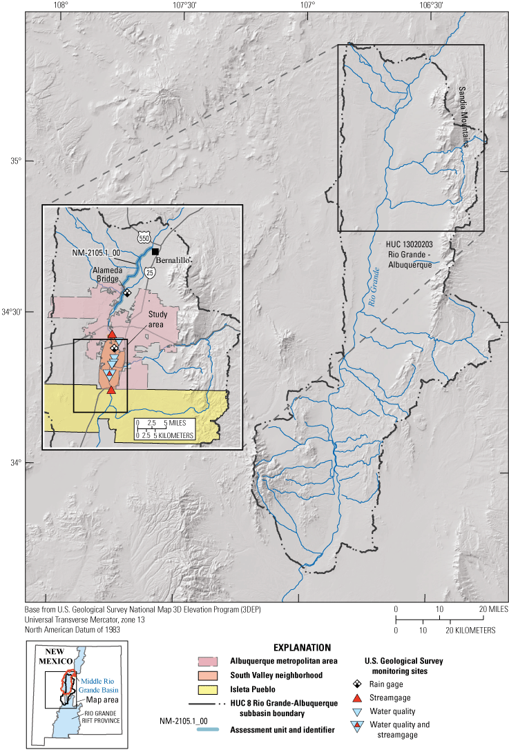
Region surrounding study area within the Rio Grande-Albuquerque hydrologic unit code (HUC) 8 and HUC 10 watersheds in central New Mexico.
Several AUs on the Rio Grande have been listed by NMED over the years as impaired by Escherichia coli (E. coli), with concentrations exceeding water-quality standards (NMEDSWQB, 2019a). Since 2010, impaired AUs in the urbanized area of Albuquerque (figs. 1 and 2) have included the following, as named and numbered by NMED:
-
Rio Grande (Alameda Bridge to U.S. Highway No. 550, 12.12 miles [mi] in length), AU identification number (ID): NM-2105.1_00
-
Rio Grande (Tijeras Arroyo to Alameda Bridge, 15.6 mi in length), AU ID: NM-2105_51
-
Rio Grande (Isleta Pueblo boundary to Tijeras Arroyo, 5.14 mi in length), AU ID: NM-2105_50
The study area extends from Bridge Boulevard (Blvd) site to the Valle de Oro site, and includes parts of the NM-2105_51 and AU NM-2105_50 AUs (fig. 2). The AU NM-2105_50 has been consistently listed as impaired for E. coli, which is why it is the focus of this study.
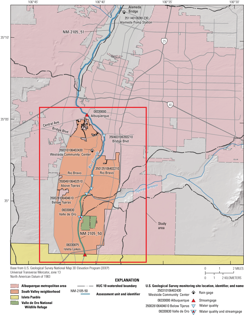
Study area in Albuquerque, New Mexico, the South Valley neighborhood and impaired assessment units (segments) of the Rio Grande. HUC, hydrologic unit code.
When these AUs were listed by NMED as impaired from E. coli, a total maximum daily load (TMDL) was then calculated for each AU. A TMDL is the calculation of the maximum amount of a contaminant allowed to enter a waterbody so that the waterbody will meet and continue to meet water-quality standards for that contaminant (EPA, 2022b). The TMDL for E. coli ranges from 1.89 × 10¹¹ colony forming units per 100 milliliters per day (cfu/100 mL/day) in low flow conditions to 5.27 × 10¹² cfu/100 mL/day in high flow conditions within the segment of the Rio Grande between Alameda Bridge and Isleta Pueblo, which includes two AUs listed above and extends upstream and downstream from the study area (NMEDSWQB, 2019b).
The New Mexico Water Quality Standard (NMWQS) 20.6.4.105 New Mexico Administrative Code (New Mexico Water Quality Control Commission, 2010) designates the Rio Grande in the study area for the following uses: irrigation, marginal warm water aquatic life, livestock watering, public water supply, wildlife habitat, and primary contact. Primary contact (NMWQS 20.6.4.900), which is defined as water use “in which there is prolonged human contact” for recreational or ceremonial purposes, has a more stringent standard for E. coli for a single sample (410 colony forming units per 100 milliliters [cfu/100 mL] or a 30-day geometric mean of 126 cfu/100 mL). NMWQS 20.6.4.105 excludes the waters of Isleta Pueblo, which has its own water-quality standards that are allowed to be lower than State standards because of their ceremonial use of water (EPA, 2021a). The Isleta Pueblo standard for E. coli for a single sample is 88 cfu/100 mL and a 30-day geometric mean of 47 cfu/100 mL for primary contact ceremonial and recreational use (EPA, 2021a).
In 2018, after implementation of best management practices in the early to mid-2010s, the northern two of these three AUs were no longer listed as impaired for E. coli on the Section 303(d) list, but the impairment listing for E. coli remained on the downstream AU, from the Isleta Pueblo boundary to the Tijeras Arroyo (NMEDSWQB, 2019a). The most downstream AU was the initial study area targeted for the project in 2019, whereas the upstream portion (Bridge Blvd to Tijeras Arroyo) was added to include an upstream area that was not listed for E. coli. However, the two upstream AUs were relisted for E. coli in 2020 following a July 2017–May 2018 study conducted by Cuidad Soil and Water Conservation Service (Fluke, 2018; NMEDSWQB, 2021). With that relisting, the study area encompassed two impaired AUs for E. coli.
While E. coli concentrations are expected to be elevated during storm events and during the wet season (July 1–October 31), results from previous monitoring, discussed in the “Previous Monitoring” section, have also shown elevated E. coli concentrations during the dry season (November 1–June 30), of up to 3,076 most probable number per 100 milliliters (MPN/100 mL) (Bosque Ecosystem Monitoring Program [BEMP], 2021). Therefore, additional information was needed to determine the E. coli source during the dry season.
The objective of this study, conducted by the U.S. Geological Survey (USGS), was to determine the extent and source of fecal-origin bacteria, in both water and bed material, within these impaired AUs of the Rio Grande during the dry season. The extent and source of fecal-origin bacteria were evaluated by using microbial source tracking (MST), a method used for identifying sources of fecal contamination in the environment. MST methods are based on the concept that intestinal systems of different warm-blooded animals have specific microbial populations to account for differences in diet and physiology. Therefore, different MST markers are associated with different sources (Francy and Stelzer, 2012). In this study, human-, canine-, and waterfowl-specific sources were evaluated.
Purpose and Scope
The purpose of this report is to evaluate the concentrations and sources, in both water and bed material, of fecal bacteria in the impaired reach of the Rio Grande. Spatial and temporal variabilities were analyzed, and instantaneous loads were calculated. Learning more about the extent of fecal-origin bacteria and its sources during the dry season will enable decision makers to focus best management practices to reduce E. coli concentrations from both point sources (discrete and discernible) and nonpoint sources (diffuse) in the Rio Grande watershed.
Study Area
The study area is in the unincorporated South Valley of Albuquerque, New Mexico (figs. 1 and 2), which is more agricultural than the metropolitan area of Albuquerque and has been for over 400 years (Visit Albuquerque, 2021). Historically, the southern part of the South Valley is more rural, and residences rely on groundwater wells and septic systems instead of city water and sewer systems. The current septic use based on Bernalillo County wastewater atlas data is estimated to be approximately 2,100 permitted systems in the South Valley and approximately 980 unpermitted systems (D. McGregor, Bernalillo County, written commun., 2022). Five water-quality sites located within two impaired AUs along the Rio Grande were sampled in this study (table 1, fig. 2).
Table 1.
Study area sites, including water-quality sampling sites, streamgages, and precipitation gages.[Horizonal coordinate information is referenced to the North American Datum of 1983. USGS, U.S. Geological Survey; NM, New Mexico; Blvd, boulevard; nr, near]
Watershed Characterization
Hydrologic unit codes (HUC) are units by which the watersheds of the United States are classified. The HUCs are defined at different levels with smaller HUCs nested within larger HUCs, from the smallest geographic area (cataloging unit) to the largest geographic area (region) (USGS, 2022a). Albuquerque and the South Valley are within the HUC 8 watershed 13020203, the Rio Grande-Albuquerque watershed, with an area of 3,216 square miles (mi2) (fig. 1). The HUC 10 watershed where the study sites are located is HUC 1302020303 (City of Albuquerque-Rio Grande, 269 mi2). Directly upstream from the sites is HUC 1302020301 (Arroyo de Las Calabacillas-Rio Grande, 330 mi2) (fig. 3). HUC 1302020302 (Tijeras Arroyo, 132 mi2) feeds into the Rio Grande between the Above Tijeras and Below Tijeras Arroyo sites (figs. 2 and 3).
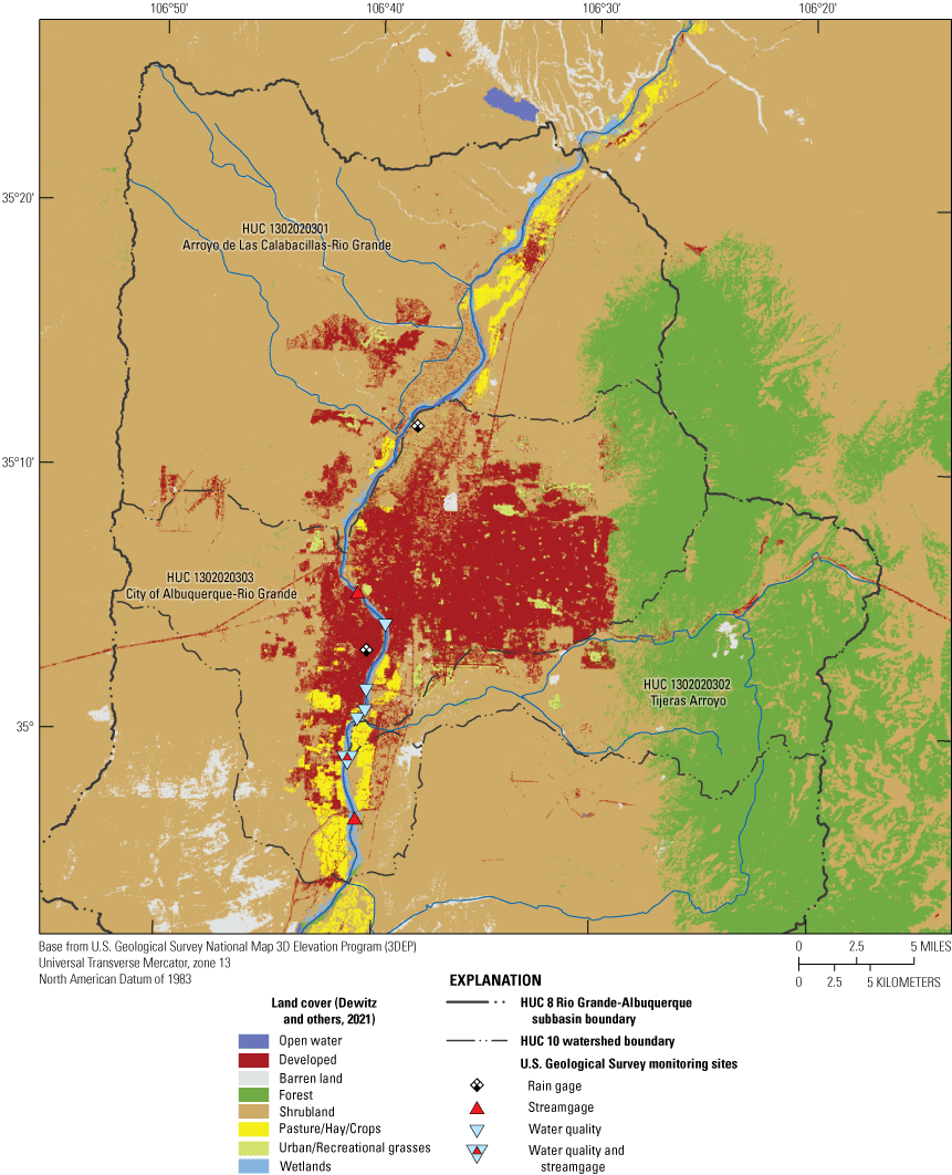
Land cover in the study area in Albuquerque, New Mexico, South Valley neighborhood. HUC, hydrologic unit code.
The three HUC 10 watersheds contributing to the study area vary in land cover (fig. 3; Dewitz, 2021). The Arroyo de Las Calabacillas-Rio Grande watershed, located directly upstream from the sites, contains 87 percent shrubland and is mostly undeveloped. The Tijeras Arroyo watershed contains approximately 94 percent shrubland and forested land. The City of Albuquerque-Rio Grande watershed is 34 percent developed and 47 percent shrubland with a small component (4 percent) of pasture, hay, and crops.
There are several potential point and nonpoint sources of E. coli in the South Valley (fig. 4). According to the EPA, sources of fecal indicator bacteria can include leaking septic systems, wastewater treatment plants, stormwater runoff, and domestic animal and wildlife waste (EPA, 2021b). On the basis of locations of existing water infrastructure, the density of water infrastructure is lower in the southeastern portion of the study area (M. Haley, Albuquerque Bernalillo County Water Utility Authority, written commun., 2021). If there is less water infrastructure in the area, it is more likely that residences will be on septic systems. LaMotte (2018) used 1990 and 2010 census data to estimate the number of people on septic systems in the coterminous United States on the basis of census blocks from the 2010 census. In the South Valley, the estimated number of people on septic systems was 13,320, as compared to the total population of 46,807 (fig. 4). However, Bernalillo County estimates that number to be much lower (approximately 3,000 systems) after initiatives to transition residences to municipal wastewater lines in the late 2000s (D. McGregor, Bernalillo County, written commun., 2022). Additional nonpoint sources similar in signature to leaking septic systems could include leaking sewer lines, sewer overflows into stormwater drains, illegal septage discharge from haulers into drains or the river, or public defecation into drainages in the study area.
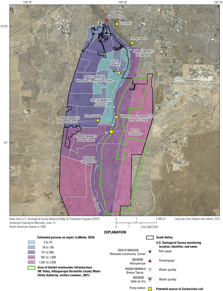
Potential sources of Escherichia coli, areas of limited wastewater infrastructure, and estimated number of persons on septic systems in the study area in Albuquerque, New Mexico, the South Valley neighborhood.
There are several point sources within the study area. A wastewater treatment plant (WWTP) is located along the Rio Grande upstream from the confluence of Tijeras Arroyo (figs. 2 and 4), which allows for a 30-day average of 47 cfu/100 mL and a daily maximum of 88 cfu/100 mL for E. coli (NMEDSWQB, 2019c). The WWTP is the largest wastewater treatment plant in New Mexico, currently treating 50 to 60 million gallons of wastewater per day (Albuquerque Bernalillo County Water Utility Authority, 2023). A dog park is located just east of the Rio Grande and upstream from Bridge Blvd. Three pump stations convey stormwater from channels and storm drainage systems throughout the city and county into the Rio Grande. The pump stations primarily contribute to the Rio Grande during storm events. One pump station is directly upstream from Bridge Blvd and two other pump stations are downstream from Bridge Blvd, one near the Westside Community Center precipitation gage and the other upstream from and to the west of the Above Tijeras site. Both downstream pump stations are operated by the City of Albuquerque (COA). The Rio Grande and its surrounding bosque (a riparian cottonwood forest) are largely designated by the COA as open space and contain a large network of trails for hiking, including dog walking (City of Albuquerque Parks and Recreation Department Open Space Division, 2014). Bernalillo County Public Works has implemented several initiatives to reduce stormwater pollution, including an initiative to reduce dog waste in the watershed (Bernalillo County, 2022) that includes dog waste depositories across the bosque. Waterfowl fecal matter can be a source of E. coli, and the Rio Grande and bosque are also a major flyway for migratory birds. Many birds inhabit the area during the winter months (typically November through March) at places like Valle de Oro National Wildlife Refuge, which is located near the southern border of the study area (fig. 2; Sullivan and others, 2009; Herzenberg, 2018).
Hydrology
The Rio Grande-Albuquerque watershed is part of the Rio Grande Rift physiographic province, with mountains forming the eastern and western boundaries. To the west, the mountains are volcanic and to the east, the mountains are uplifted igneous and sedimentary geologic units. The valley floor consists of compacted sands and gravels of the Santa Fe Group, which is Paleogene in age and locally includes Quaternary aged alluvium (Natural Resources Conservation Service, 2002).
The Santa Fe Group aquifer is an unconfined aquifer that underlies the Rio Grande, and the depth to groundwater varies widely throughout the Middle Rio Grande Basin (fig. 1), a geologic basin that contains the study area (Bartolino and Cole, 2002). The Santa Fe Group thickness ranges from 1,400 to 14,000 feet (ft), and the depth to groundwater ranges from less than 2 ft near the Rio Grande, where groundwater and surface water are closely connected (Bartolino and Cole, 2002), to about 1,200 ft in areas west of Albuquerque.
In the Rio Grande-Albuquerque watershed, the Rio Grande is a highly regulated system with the flow controlled by dams and reservoirs upstream and downstream from the study area. Flow in the Rio Grande varies widely throughout the year, with the highest flows typically occurring during spring snowmelt (Bartolino and Cole, 2002). Discharges in 2020 and 2021 were historically low during the dry season and were often statistically below the 25th percentile (548 cubic feet per second [ft3/s]) of historical flows at USGS 08330000 (Albuquerque) (fig. 5; Jian and others, 2008). Discharges for 53 percent of the days during the dry season were below the 25th percentile from November 1, 2019, through June 30, 2020, and those for 63 percent of days during the dry season were below the 25th percentile from November 1, 2020, through June 30, 2021. When the flow is very low at USGS 08330830 (Valle de Oro), diurnal fluctuations based on the effluent discharge can be observed.
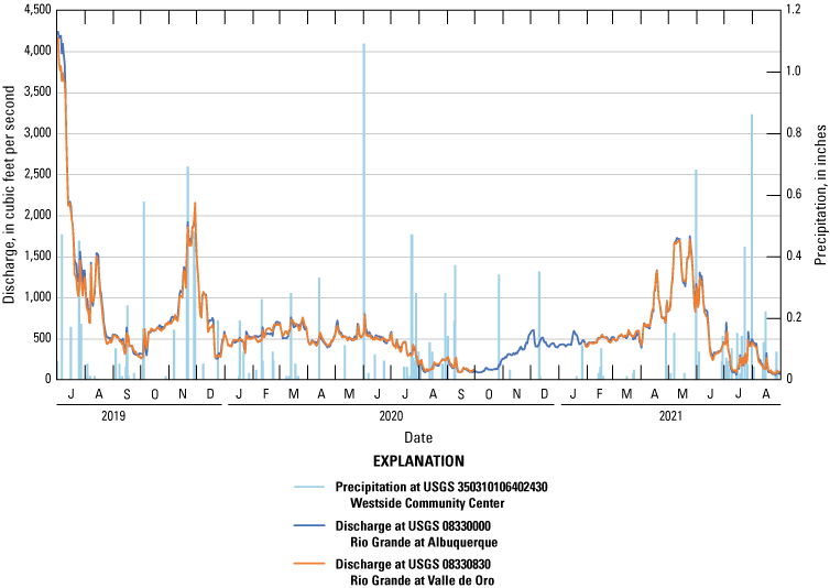
Discharge at U.S. Geological Survey (USGS) 08330000 Rio Grande at Albuquerque and USGS 08330830 Rio Grande at Valle de Oro and precipitation at USGS 350310106402430 Westside Community Center during the duration of the study. Data from USGS (2021).
An intricate system of riverside drains, irrigation canals, and community irrigation ditches known as acequias line the Rio Grande. The irrigation canals and ditches are primarily used during irrigation season in places where water from the river is diverted by the Middle Rio Grande Conservancy District (Bartolino and Cole, 2002). The riverside drains parallel both sides of the river and capture lateral groundwater flow derived as seepage loss from the river and irrigation return flow (as shallow groundwater flow), which help keep the river at a stable level.
Within the study area, the main tributaries of the Rio Grande are the WWTP effluent outfall, which was considered a tributary inflow because the water is originally drawn from the Santa Fe aquifer system (fig. 4; Bartolino and Cole, 2002), and Tijeras Arroyo. With its 132 mi2 drainage area, Tijeras Arroyo is one of the largest arroyos in the Albuquerque area and is intermittent in flow, typically during storms. At streamgage USGS 08330600 Tijeras Arroyo near Albuquerque, N. Mex., discharge was measured during only 40 days in 2021 (USGS, 2022b). Tijeras Arroyo serves as the primary channel for snowmelt and stormwater from areas east of the Sandia Mountains (fig. 1; City of Albuquerque Parks and Recreation Department Open Space Division, 2014). Although not widely reported on, Tijeras Arroyo does contribute a notable amount of sediment into the Rio Grande during storm events. During flash floods between 1937 and 1947 (Copeland, 1995), 26 suspended sediment samples were collected from Tijeras Arroyo. The average suspended sediment concentration for Tijeras Arroyo was 58,000 milligrams per liter (mg/L) at an average discharge of 300 ft3/s, and the average size class breakdown was 19 percent clay, 69 percent silt, and 12 percent sand.
Climate
The climate in this study area is semiarid, with mostly sunny days and low humidity (Thorn and others, 1993). From water year 2015 through 2021, annual precipitation ranged from 5.19 to 10.13 inches (in.) at the Alameda Pump Station precipitation gage in northern Albuquerque (table 1, fig. 2) and from 4.70 to 10.61 in. at the Westside Community Center precipitation gage in southern Albuquerque (table 1, fig. 2; USGS, 2021). In the Middle Rio Grande Basin, the rainy season is from July through October, with 45–62 percent of annual precipitation falling within those months. Thunderstorms tend to be localized and short lived, making the precipitation spatially and temporally variable throughout the Middle Rio Grande Basin (Bartolino and Cole, 2002).
Previous Monitoring
Since the mid-2000s, several entities, including Bernalillo County, the Albuquerque Metropolitan Arroyo Flood Control Authority, and the COA have monitored E. coli and its sources in the study reach and the surrounding watershed. Data associated with these studies that fall within the parameters of the current study, specifically, samples collected from sites in or near the study reach and samples collected during the dry season, are compiled in Travis (2023). A 2005 study utilized ribotypes and antibiotic resistance profiles to determine sources of E. coli in the Rio Grande, and the results indicated a variety of sources, with the predominant ones being avian and canine (Parsons Water & Infrastructure, Inc., 2005). In a 2018 study, the COA contracted Daniel B. Stephens and Associates, Inc., to study fecal bacteria and its sources in the Rio Grande as it runs through the city (COA, 2019); genetic markers indicated that avian and human sources were the largest contributors of fecal-origin bacteria to the river during nonstormwater events. E. coli was detected in all 12 dry season samples and ranged from 10 to 336 MPN/100 mL, where MPN/100 mL is assumed to be equivalent to cfu/100 mL (Noble and others, 2004). The highest E. coli concentration (336 MPN/100 mL) was detected at Rio Grande at the Isleta Pueblo northern boundary (figs. 1 and 2; COA, 2019).
Fluke (2018) and Fluke and others (2019) evaluated E. coli levels in water and riverbed sediments in the Rio Grande from Bernalillo, N. Mex., to the Valle de Oro site. During the dry season, E. coli concentrations in water ranged from 150 to 1,660 cfu/100 mL at Albuquerque and from 20 to 1,840 cfu/100 mL at the Valle de Oro site. Riverbed sediments were collected at Albuquerque and Rio Bravo and ranged from 0.01 to 249.93 most probable number per 100 grams of dry weight sediment (MPN/100 gDW) and 2.69 to 1,538.7 MPN/100 gDW, respectively, during the dry season (Fluke, 2018, Fluke and others, 2019).
Fluke and others (2019) suggested that the fine-grained bed sediment could be a reservoir for bacteria that could provide suitable habitat for regrowth, resulting in resuspension and higher concentrations of bacteria in this reach. The possibility of regrowth in these fine sediments should be considered when creating best management practices emplaced to reduce the nonpoint sources of bacteria. Sanders and others (2013) suggested that assessment of factors such as interaction with sediment, bacteria regrowth, and sources are important when studying elevated bacteria during baseflow conditions. To study E. coli concentrations in a comparable system, Paretti and others (2019) installed piezometers in the hyporheic zone of the Santa Cruz River, Arizona, to sample waters below the stream channel from the middle of the bed to the wetted edge and found that the E. coli concentrations had both a vertical and horizontal gradient that could contribute to mass E. coli loading during flooding situations.
Additionally, E. coli monitoring has been ongoing in the study reach of the Rio Grande by the Middle Rio Grande Stormwater Quality Team and Isleta Pueblo. The Middle Rio Grande Stormwater Quality Team sampling is conducted by BEMP, and results are available through their website (BEMP, 2021). BEMP sampling followed the New Mexico Environment Department Surface Water Quality Bureau bacteriological sampling standard operating procedure, which suggests that sampling occur from one point in the river that is well mixed and more than 6 in. deep (NMEDSWQB, 2022b). From 2017 through 2020, the BEMP documented E. coli concentrations ranging from 10.7 to 3,076 MPN/100 mL during the dry season, with the maximum value of 3,076 collected after a storm event. Isleta Pueblo also conducts sampling, and the results are accessible through the Water Quality Data Portal (National Water Quality Monitoring Council, 2021). The Isleta Water Quality Standards indicate that bacteriological samples are collected at a point where there is adequate vertical and lateral mixing (EPA, 2021a). From 2017 through 2020, Isleta Pueblo documented E. coli concentrations ranging from 5.2 to 2,098 MPN/100 mL during the dry season.
Methods
For the duration of the study, water and bed material samples were collected from five sites along the Rio Grande between the USGS gages at Albuquerque (08330000, Rio Grande at Albuquerque), to the northern border of the Isleta Pueblo (08330875, Rio Grande at Isleta Lakes; fig. 2). Water was analyzed for E. coli, MST, and suspended sediment analysis, and bed material was analyzed for E. coli and MST markers. All water-quality, sediment, discharge, and precipitation data are publicly available from the USGS National Water Information System (USGS, 2021) using the USGS site numbers in table 1.
Field Methods
Discrete surface-water samples, bed material samples, and field parameters were collected from five sites along the Rio Grande between April 2020 and August 2021 (table 1). Within the river cross section at each site, samples were collected from within 5 ft of the east bank, river center, and within 5 ft of the west bank to determine if there was heterogeneity within the sampling site. These east, center, and west sampling locations will collectively be referred to as “three-point sampling” at each site. This sampling method is atypical of the suggested bacteriological sampling method specified by the New Mexico Environment Department Surface Water Quality Bureau Standard Operating Procedure 9.1, where compliance sampling typically occurs at only one well-mixed location within the stream (NMEDSWQB, 2022b). Twelve sampling events occurred at each of the sites, six events in 2020 and six events in 2021. Four sampling events each year occurred during the dry season and two sampling events each year either occurred during the wet season or during the dry season at a discharge of greater than 1,000 ft3/s.
Dry season sampling criteria for this study have been set by evaluating (1) past sampling conditions in relation to precipitation and discharge and (2) the National Pollutant Discharge Permit for the WWTP (NMEDSWQB, 2019c). The dry season, as defined by the permit, is November 1–June 30; wet season sampling, which occurs after a rain event during the time period of July 1–October 31, is defined as occurring when rainfall is greater than 0.25 in., and an antecedent dry period of at least 48 hours after a rain event greater than 0.1 in. in magnitude (NMEDSWQB, 2019c). Given the criteria of the permit for the dry season and the peaks in flow in the Rio Grande after snowmelt over the past few years, dry season sampling occurred when the following criteria were met within the greater Albuquerque area:
-
sampling event is between November 1 and June 30,
-
at least 48 hours after a rain event of less than 0.25 in., and
-
Rio Grande discharge is less than 1,000 ft3/s.
USGS precipitation and streamgages within the study area were used to monitor the streamflow and rainfall sampling criteria.
Three-point sampling surface-water samples for E. coli, MST markers, and suspended sediment concentration were collected using the discrete or grab method. The USGS National Field Manual states that the isokinetic depth integrated sampling is the standard procedure and typically is the preferred method if the cross section is uneven in velocity and (or) depth (USGS, variously dated). Additionally, isokinetic samples are composited into a churn that is not able to be autoclaved, so bacteria samples are traditionally collected as a grab sample. However, Paretti and others (2018) directly compared samples collected using the isokinetic depth integrated sampling technique to grab samples and found similar E. coli and suspended sediment concentrations using both methods. Therefore, this study used the grab sample technique.
Water and bed material samples for E. coli and MST markers were collected by following the USGS protocols described in Myers and others (2014). Before going into the field for sample collection, bottle kits containing the appropriate sterilized 1-liter (L) wide-mouth polyethylene bottles and sediment jars were assembled. At a minimum, all sampling equipment was soaked in phosphate free detergent for 30 minutes and rinsed with tap water followed by deionized water (USGS, 2004). After the initial cleaning step, the E. coli sampling bottles were autoclaved, and the MST marker sampling bottles and jars were sterilized with a sodium hypochlorite solution, neutralized with a sodium thiosulfate solution, and rinsed with sterile deionized water (Myers and others, 2014).
To prevent contamination, the least amount of equipment was used to collect a sample, and sample collection followed the USGS National Field Manual for bacteria sample collection (USGS, variously dated). If the sites were safely wadable, the sampling bottle was submerged to allow the bottle to fill with the opening pointed slightly upward toward the current. If the sites were not wadable, the samples were collected either from a bridge (Bridge Blvd and Rio Bravo) using a DH–95 sampler and a bridge board, or, at the sites with no accessible bridge (Above Tijeras, Below Tijeras, and Valle de Oro), the grab samples were collected from a kayak. All water samples were collected with about 2.5–5 centimeters of headspace in each bottle to allow for proper mixing. The E. coli and MST marker samples were bagged immediately to prevent contamination and stored on ice in a cooler until analysis.
Bed sediment samples were analyzed for E. coli and MST markers at the Ohio Water Microbiology Laboratory (OWML) and for fine sand break at the New Mexico Water Science Center (NMWSC) Sediment Laboratory. For the E. coli and MST bed sediment collection, three sterile, plastic, wide-mouth 125-milliliter (mL) jars were used at each sampling location. For the fine sand break analysis, a 16-ounce plastic jar was used. The lidded sampling jar was lowered to the river bottom where the lid was removed to scoop bed sediment into the jar. The lid was then secured tightly on the jar before bringing the jar to surface. The jars were bagged immediately to prevent contamination and stored on ice in a cooler until analysis. When river stage was too high to easily sample by hand, a tool with a hose clamp attached to a long handle was used to hold the sample jar and scoop bed sediment from the river bottom.
Four known-source fecal samples were collected from fresh material and of known origin. Solid samples were collected for geese (n=2) and canine (n=1) sources. One human source, a wastewater influent sample, was collected from the WWTP. All known-source fecal samples were stored on ice immediately after collection and shipped to the OWML for processing within 24 hours. Known-source samples were only collected once throughout the study.
Physical parameters, including water temperature, pH, specific conductance, dissolved oxygen, turbidity, and barometric pressure, were recorded at each three-point sampling location within each site using either a Yellow Springs Incorporated 6920 series or 600 series multiparameter water-quality sonde (YSI Incorporated, Yellow Springs, Ohio) or an In-Situ Aqua TROLL 600 (In-Situ Inc., Fort Collins, Colorado). Following the manufacturer instructions and USGS methods, a calibration check was performed on the sonde each morning before collecting samples (USGS, variously dated). Field parameters, including turbidity, dissolved oxygen, specific conductance, pH, and water temperature, were measured by USGS staff. Two USGS streamgages, Albuquerque and Valle de Oro, provided continuous discharge throughout the study (table 1). Daily mean discharge from Albuquerque was used for the Bridge Blvd and Rio Bravo sampling sites. Daily mean discharge from Valle de Oro was used for the Above Tijeras and Below Tijeras sampling sites, as it reflects the daily effluent outfall fluctuations from the WWTP, which is upstream from Above Tijeras. At Valle de Oro, discharge was measured during every sampling date to check the continuous streamgage at the site. Table 2 shows the discharge measurements associated with each site for each sampling event. Discharge measurements were collected using standard USGS protocols as described in Rantz and others (1982), Nolan and Shields (2000), and Turnipseed and Sauer (2010).
Table 2.
Daily mean discharge values used for all events at five sites on the Rio Grande in Albuquerque, New Mexico.[Data from U.S. Geological Survey (USGS, 2021). Dates shown as month/day/year. Sample times shown in 24-hour format. All sample times are local. ft3/s, cubic foot per second; Blvd, boulevard]
Analytical Methods
The analytical methods for E. coli and MST in both water and bed material and suspended sediment analysis in water are discussed in this section.
Escherichia coli in Water
Water samples were analyzed for E. coli by USGS staff within 6 hours of sample collection using the colilert method (Standard Methods Committee of the American Public Health Association, American Water Works Association, and Water Environment Federation, 2022; USGS, variously dated). The 1-L samples collected for E. coli were shaken prior to pouring 100 mL of sample into a sterile graduated cylinder. From the cylinder, the sample was immediately poured into a sterilized 100-mL bottle, and a reagent packet was poured into that bottle. The bottle was then shaken again until all the reagent was dissolved, and the sample was poured into a Quanti-Tray and sealed with an IDEXX Quanti-Tray Sealer PLUS (IDEXX Laboratories, Inc., Westbrook, Maine) and incubated at 35 degrees Celsius (°C) for 24–28 hours. After the incubation period, the E. coli density was calculated by counting the number of small and large wells whose water sample reacted with the reagent on the Quanti-Tray under a long-wave ultraviolent light at 365 nanometers. The colilert method reported results as MPN/100 mL, which has been evaluated to have a 1:1 relationship to results reported in cfu/100 mL (Noble and others, 2004).
Microbial Source Tracking Markers in Water
Samples were analyzed for MST markers at the OWML. Within 24 hours of sample collection, varying matrix-dependent volumes of water samples were filtered onto 0.4-micrometer polycarbonate filters (Whatman, Inc., Florham Park, New Jersey). The filters were aseptically placed into 2-mL screw cap vials containing 0.3 grams (g) of sterile glass beads (Sigma-Aldrich Corp., St. Louis, Missouri) and preserved at −70 °C. Filtered samples underwent deoxyribonucleic acid (DNA) extraction by use of the DNA-EZ extraction kit (GeneRite, Monmouth Junction, N.J.) and extracts were stored at 4 °C until analysis by quantitative polymerase chain reaction (qPCR) within 7 days of extraction. qPCR was analyzed using either a StepOnePlus or a QuantStudio 3 Real-Time PCR System (Thermo Fisher Scientific, Waltham, Massachusetts) on the basis of conditions reported in the references for the following MST markers:
-
human-associated Bacteroides marker (human marker, HF183/BacR287) (Green and others, 2014),
-
canine-associated Bacteroides marker (canine marker, BacCan) (Kildare and others, 2007), and
-
waterfowl-associated Helicobacter marker (waterfowl marker, GFD) (Green and others, 2012).
MST Quality Control
Quality control analyses and procedures are vital to the production of reliable microbial source tracking data. In addition to field blanks collected onsite, several types of blank samples were created during the analytical process:
-
filter blank—sterile, buffered water filtered at the same time as the samples at the OWML,
-
extraction blank—sterile vial containing only acid-washed beads was DNA-extracted along with each batch of samples, and
-
qPCR blanks (no template controls)—sterile, molecular-grade water was used instead of sample DNA extract as qPCR template.
All samples were analyzed by qPCR in duplicate; final results represent an average of duplicate qPCR reactions. Potential matrix effects on the qPCR were evaluated by analyzing a portion of each sample that was spiked with a known quantity of target DNA. If matrix inhibition was observed, sample DNA extracts were diluted accordingly and then processed by qPCR.
Each qPCR run included a seven-point standard curve run in duplicate (serial dilutions of known quantities of target DNA). MST marker concentrations for unknown samples were interpolated from the standard curves by converting qPCR output (cycle threshold values).
MST Data Qualifications
A limit of detection was established for each MST qPCR assay. The limit of detection was the lowest concentration detected with 95-percent confidence. If detections were found in the blank samples, the limit of blanks was calculated. If the limit of blanks had a higher concentration than the limit of detection, the limit of blanks was used as the detection limit. Results for samples that were below either limit were reported as less than (<) the detection limit.
Low-level quantification can be unreliable. To avoid misinterpretation of unreliable results, a limit of quantification was established for each assay. The limit of quantification was established by using the average cycle threshold value of the limit of detection and subtracting two times the standard deviation of those cycle threshold values. The result for a sample that detected the target DNA and was above the limit of detection but below the limit of quantification was reported with an “E” to denote that it was an estimated value. Along with the “E,” there may also be a value qualifier. The “b” value qualifier meant that the reported concentration was extrapolated below the limit of quantification but is above the limit of detection. The “~” value qualifier meant that the duplicate qPCR results do not agree.
Escherichia coli Bacteria and Microbial Source Tracking Markers (Human-, Canine-, and Waterfowl-Specific Sources) in Bed Material
River-bottom sediment samples were analyzed for concentrations of E. coli bacteria and MST markers (human-, canine-, and waterfowl-specific sources) at the OWML by the methods described in the section “Microbial Source Tracking Markers in Water.” Processing steps for sediment samples (Francy and Darner, 1998) were required before analysis. Briefly, a 30-g aliquot of composited sediment from the three subsamples was placed into a bottle containing 300 mL of sterile phosphate buffer; a second aliquot of composited sediment was reserved to determine percent dry weight. The bottle was placed on a wrist-action shaker for 45 minutes, then removed; suspended materials were allowed to settle for 30 seconds, and the liquid phase was decanted for analysis (filtration for MST marker analysis and analysis by colilert). After E. coli and MST analyses were completed, calculations were made to convert MST marker (copies) and E. coli (MPN) results to copies or MPN/gDW.
Suspended Sediment in Water
Suspended sediment concentration in the water column was measured by the USGS NMWSC Sediment Laboratory following the Quality-Assurance Plan for the Analysis of Fluvial Sediment (Stiles, 2006). Once received, samples were stored in a cool, dark location, allowed to settle for 2 weeks, and analyzed within 60 days. Depending on the amount of sand or clay in the sample, either the filtration method or the evaporation method described in ASTM D3977–97 (American Society for Testing and Materials, 2019) was used for analysis.
If the evaporation method was used, the sample was washed in an evaporation dish, dried, and weighed. If the dissolved-solids concentration was greater than 2,300 mg/L and the concentration of sediment was less than 200 mg/L, then a dissolved-solids correction needed to be applied. If the filtration method was used, the sample was poured into a crucible, vacuum pressured, and forced through a filter. The crucible was then dried, cooled, and weighed. No mathematical adjustments were needed if the filtration method was used. For both the evaporation and filtration method, concentrations were calculated using the Sediment Laboratory Environmental Data System (Stiles, 2006).
Particle Size in Bed Material
Sand-fine analysis was performed on bed material samples at the NMWSC Sediment Laboratory following the Quality-Assurance Plan for the Analysis of Fluvial Sediment by the NMWSC Sediment Laboratory (Stiles, 2006). The fine analysis refers to the percentage of particles that pass through a 0.062-millimeter (mm) sieve, and the sand analysis refers to the percentage of particles remaining on that sieve. Following the recommendations of Guy (1969) and Tyler Industrial Products (1976), the dry sieve method was used for this analysis with a W.S. Tyler Ro-Tap machine. First, the sand and gravel were separated from the silt-clay fraction by wet sieving. Next, the sand and gravel were dried and weighed. The sample was shaken in the W.S. Tyler Ro-Tap machine for 20 minutes, and then the size-fraction weights that remained in each sieve were entered into the Sediment Laboratory Environmental Data System (Stiles, 2006). If the sample weighed more than 400 g, the sample was split into two samples for analysis on the Ro-Tap machine.
Data Analysis Methods
The replicate pair variability was analyzed in different ways depending on the analyte. In describing the “two-range model,” Mueller and others (2015) state that over low concentrations, standard deviation (SD) is generally uniform, but at higher concentrations, relative standard deviation (RSD) is more uniform than SD. Paretti and others (2018) reported extensively on quality control and assurance methods for bacteria sampling methods and with a large amount of E. coli replicates, were able to analyze the variability in sampling methods using the bias-corrected log-log regression model (Mueller and others, 2015). Because of the lower number of replicate pairs and relatively higher concentrations for all parameters, RSD was used instead of SD to study variability for all analytes,
whereCenvironmental
is the environmental sample concentration, and
Creplicate
is the replicate sample concentration.
For E. coli and suspended sediment, which had some lower concentrations, SD was also calculated. Results for many analytes were censored (that is, less than the reporting level) in one or both replicate samples, which excluded them from replicate analysis.
Instantaneous or mean daily loading rates, also known as flux, for E. coli and MST markers were calculated using a simple approach (Meals and others, 2013) of multiplying concentration times discharge and were reported in units of MPN or copies per day,
whereK
is the unit conversion factor (2.45×10⁷ when calculating mean daily flux in most probable number per day [MPN/day] or copies per day [copies/day], which accounts for conversions of cubic feet to milliliters [1 cubic foot equals 28,316.8 mL] and seconds to days [86,400 seconds equal 1 day]),
Q
is discharge (in cubic feet per second), and
C
is concentration (MPN or copies per 100 mL).
The mean daily flux is the instantaneous rate at which the load passes a point in the river. This flux is not equal to the load, which is the mass of a substance passing through a specific point in the river. The load is calculated over a specified timeframe with frequent monitoring. Because of the infrequency of the sampling and targeting of dry season, lower-flow events, accurate loads cannot be calculated.
To categorically compare fluxes of different microbiological constituents at a single site and across multiple sites, the mean daily fluxes were divided into five bins (Bushon and others, 2017). For each constituent, regardless of flow conditions, all results were combined, ranked, and binned. All nondetects were assigned to the 0 bin. Bins 1–4 contained an equal number of sample results per bin, with the highest fluxes placed in bin 4. Table 3 lists the ranges of daily fluxes per bin for each constituent. Once the bins were established, each sample result for a given constituent was assigned a bin number that was then separately averaged for each site for dry and wet season samples. Average bin scores can be used to compare the fluxes of a single constituent across sites and to compare the fluxes of different constituents at a single site.
Table 3.
Range of mean daily fluxes per bin for Escherichia coli and microbial source tracking markers.Statistical analyses were conducted in the R statistical computing environment (R Core Team, 2022). Because a high percentage of MST marker data were censored values, summary statistics were calculated for censored data using the “censtats” function in the Nondetects and Data Analysis (NADA) software package, and the summary statistics using the regression on order statistics method were reported for this study. Boxplots were created by using the “cenboxplot” function from the NADA software package (Lee, 2020) in the R statistical computing environment (R Core Team, 2022). Boxplots for analytes with censored data were grouped by sample type; percentiles were estimated by using the robust regression on order statistics method (Helsel, 2012). Outlier data points on boxplots were defined for this study as greater than 1.5 times the interquartile range. To evaluate correlations, Pearson’s r and Kendall’s tau were calculated for uncensored data, and only tau was calculated for censored data. All E. coli concentration data were log10 transformed before conducting the Pearson’s r calculations because the bacteria data were not normally distributed. Strong linear correlations of r = 0.9 or above typically correspond to tau values of about 0.7 or above (Helsel and others, 2020). For uncensored data, the base R function “cor.test” was used to determine correlations using both Pearson’s r and Kendall’s tau, and for censored data the “cenken” function was used from the NADA package to determine Kendall’s tau (Lee, 2020). When evaluating differences between the datasets, Kruskal-Wallis rank sum test was used for uncensored data using base R function “kruskal.test,” and when a probability value (p-value) was less than 0.05, the differences were found to be significant. If significant differences were found, then to determine if three-point sampling locations within sites differed from others for the uncensored data, Dunn’s test using the Benjamini & Hochberg correction method was used using the R package “PMCMRplus” and its “kwAllPairsDunnTest” function (Pohlert, 2021). To evaluate differences between three-point sampling locations within sites for uncensored data, the “cen1way” function from the NADA2 package was used (Julian and Helsel, 2021), which performs the Peto-Peto nonparametric test of differences.
Data-Quality Assurance and Assessment
Quality control and assurance samples were collected in the field to ensure the field sample collection methods and field environment did not introduce contamination into the sampling process and to determine the variability in the sample collection process and laboratory methods.
Field blanks were collected at each a field site by pouring sterile phosphate buffer water with magnesium chloride directly into a sterilized 1-L poly sample collection bottle. The field blanks were analyzed to assess the equipment and field activities for any contamination potentially introduced into the samples during the cleaning and sampling process. Six field blanks were collected and analyzed for E. coli and MST markers. One source solution blank was analyzed for E. coli and was collected in the laboratory by directly pouring the buffer water into the sterilized graduated cylinders used for measuring out the sample for processing. All field and source blanks had no detections of E. coli or MST markers.
Six replicate water samples and three replicate bed material samples (table 4) were collected sequentially. Sequential replicates assessed the variability of samples resulting from field activities as well as laboratory analysis. Five replicate water samples from the east bank of Above Tijeras were collected on April 27, 2020, June 10, 2020, July 23, 2020, March 3, 2021, and June 23, 2021, and analyzed for E. coli, MST markers, and suspended sediment. A water replicate from the east bank location at Bridge Blvd was collected on May 18, 2021, and analyzed for E. coli and suspended sediment only. Bed material replicate samples from the east bank location at Above Tijeras were collected on June 10, 2020, March 3, 2021, and June 23, 2021, and analyzed for E. coli and MST markers.
Table 4.
Replicate samples and their calculated standard deviations and relative standard deviations for seven samples collected on the Rio Grande in the Albuquerque, New Mexico, area during 2020–21.[Dates shown as month/day/year. SD, standard deviation; RSD, relative standard deviation; E. coli, Escherichia coli; MPN/100 mL, most probable number per 100 milliliters; NC, not calculated; mg/L, milligram per liter; copies/100 mL, copies per 100 milliliters; E, estimated value; <, less than; --, no value; MPN/gDW, most probable number per gram of dry weight sediment; copies/gDW, copies per gram of dry weight sediment; Blvd, boulevard]
On the basis of the two-range model, low-range SDs were calculated for E. coli at concentrations below 150 MPN/100 mL and for suspended sediment concentrations below 100 mg/L. High-range RSDs were calculated for all other analytes. For the replicate water sample results, the average RSDs were less than 20 percent for most analytes, except for the human marker (44.1 percent) and the canine marker (28.3 percent). The average SD was 3.3 MPN/100 mL for low-range E. coli replicates and 10.1 mg/L for low-range suspended sediment concentration replicates. Bed material samples were mostly below the reporting level, but for the E. coli and human marker replicate pairs where RSDs could be calculated, the averages were 15.9 MPN/gDW SD for E. coli replicates and 24.5 percent RSD for the human marker.
Known-source fecal samples were collected and analyzed to verify the analytical performance of the MST markers used in the study. Analysis of all known source samples resulted in detections of the associated MST marker (table 5). Analysis of wastewater influent from the WWTP resulted in detection of the canine marker in addition to the human marker, and the analysis of the waterfowl marker also included detection of the canine marker. This was not unexpected because fecal bacteria may be transferred between host species living in close contact, resulting in co-occurrence of host-associated MST markers in a sample (Field and Samadpour, 2007; Stewart and others, 2007; Roslev and Bukh, 2011). Concentrations of MST markers in cross-reacting samples were lower than in target samples except in the case of the second Canada goose sample, as shown in table 5.
Table 5.
Reported values of microbial source tracking (MST) markers from known-source samples collected near Albuquerque, New Mexico, for MST.[Dates shown as month/day/year. Values in bold typeface indicate samples where the concentration was above the limit of detection (LOD). The LOD for a given sample is represented by less than (<) a concentration when a nondetect occurred. The LOD varies per assay and is defined as the lowest concentration detected with 95-percent confidence]
Characterization of Escherichia coli Microbial Source Tracking Markers and Other Parameters in Water and Bed Material
The following discussion provides an overview of the findings in water and bed material. Physical parameters, suspended sediment concentrations, E. coli, and MST markers were evaluated and summarized. E. coli concentrations in water were compared to water-quality standards. The fluxes for E. coli and MST markers in water were calculated for all sites and locations. Bed material E. coli and MST marker concentrations were also evaluated, and particle size was reviewed to determine if there was fine material providing an opportunity for bacteria regrowth. Water and bed material data were then evaluated to determine if there were any temporal (dry versus wet season) and spatial (sample site and location) differences. Lastly, MST marker concentrations were ranked to determine the dominant sources of fecal bacteria at the different sites.
Physical Parameters and Suspended Sediment Characterization in Water
Physical parameters, including pH, specific conductance, dissolved oxygen, and turbidity, were evaluated at each sample site and three-point sampling location (fig. 6). There was minimal fluctuation in values between each of the three-point sampling locations at the Bridge Blvd and Rio Bravo sites but also between the Bridge Blvd and Rio Bravo sampling groups. As expected, the effluent outfall affected several of the physical parameters after it entered from the east bank upstream from the Above Tijeras site and continued downstream to the Valle de Oro site. Specific conductance increased from a median of 333 microsiemens per centimeter at 25 degrees Celsius (µS/cm at 25 °C) at the west bank to 587 µS/cm at the east bank at Above Tijeras, whereas the median ranged from 331 to 334 µS/cm at Bridge Blvd and Rio Bravo upstream from the effluent outfall. pH decreased at the east bank at Above Tijeras to a median of 7.5 as compared to the median from the upstream sites at Bridge Blvd and Rio Bravo, which ranged from 8.2 to 8.3. Median dissolved oxygen concentrations ranged from 8.1 to 8.3 mg/L upstream at Bridge Blvd and Rio Bravo versus the east bank of Above Tijeras where the median dissolved oxygen concentration was 7.8 mg/L. The median turbidity ranged from 53 to 64 formazin nephelometric units (FNU) at Bridge Blvd and Rio Bravo, and the median turbidity at east bank at Above Tijeras was 39 FNU. The influence of the effluent on the east bank samples continued to be visible at the downstream sites Below Tijeras and Valle de Oro, with medians of 49 and 75 FNU, respectively, and lower than the other three-point sampling locations at those sites.
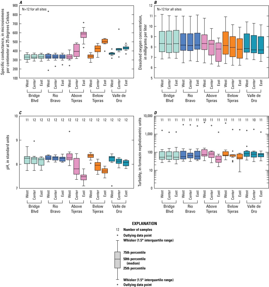
Boxplots showing physical parameters including A, specific conductance, B, dissolved oxygen, C, pH, and D, turbidity from all sampled events at five sites on the Rio Grande in Albuquerque, New Mexico.
Suspended sediment concentrations (fig. 7A) were similar at Bridge Blvd and Rio Bravo and at the west and center locations at Above Tijeras, with median values ranging from 138 to 177 mg/L. At the east bank at Above Tijeras, suspended sediment concentrations decreased to a median value of 103 mg/L. Suspended sediment concentrations increased along the west bank at Below Tijeras, with a median of 185 mg/L and a maximum value of 2,990 mg/L. Valle de Oro suspended sediment concentrations showed more consistent mixing in the cross section, ranging from median values of 136 to 198 mg/L.
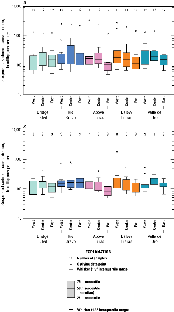
Boxplots showing suspended sediment concentrations from A, all sampled events and, B, dry season only events at five sites on the Rio Grande in Albuquerque, New Mexico.
Escherichia coli Characterization in Water
E. coli concentrations vary between the dry season and the rest of the year. Table 6 contains summary statistics for E. coli, including mean, median, maximum, and minimum values of all the data and only the dry season data. Figure 8A–E shows time series plots of E. coli and MST marker concentrations for each site and sampling location. Figures 9 and 10 show boxplots for all data collected at each site and sampling location and data collected during the dry season only, respectively. Median E. coli values ranged from 42 to 160 MPN/100 mL for all samples, and from 32 to 120 MPN/100 mL for dry season samples (table 6). The west sample location had the highest concentrations collected at Above Tijeras (during the dry season, fig. 10) and Below Tijeras (all data, fig. 9), which were an order of magnitude higher in concentration than those of other samples. These higher values during the dry season could be indicative of an increase of fecal contamination on the west side of the river during the event.
Table 6.
Summary statistics for Escherichia coli (E. coli) in water for all samples, for samples collected during the dry season only, and for E. coli in bed material during the dry season.[Data from U.S. Geological Survey (USGS, 2021). MPN/100 mL, most probable number per 100 milliliters; MPN/gDW, most probable number per gram dry weight; Blvd, boulevard]
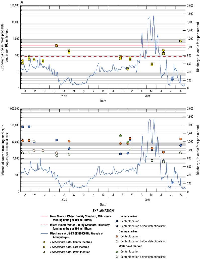
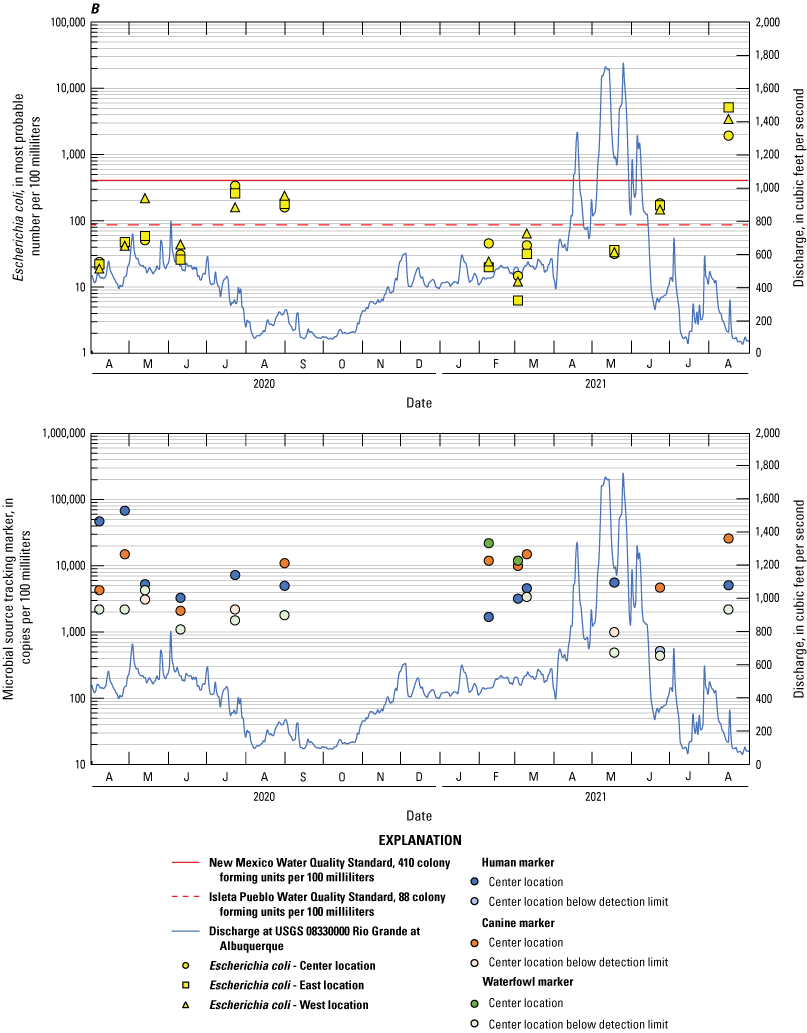
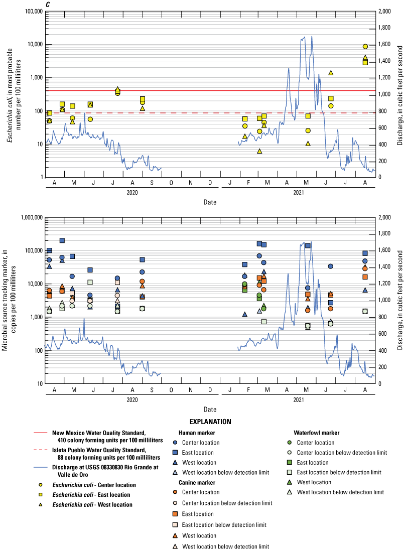
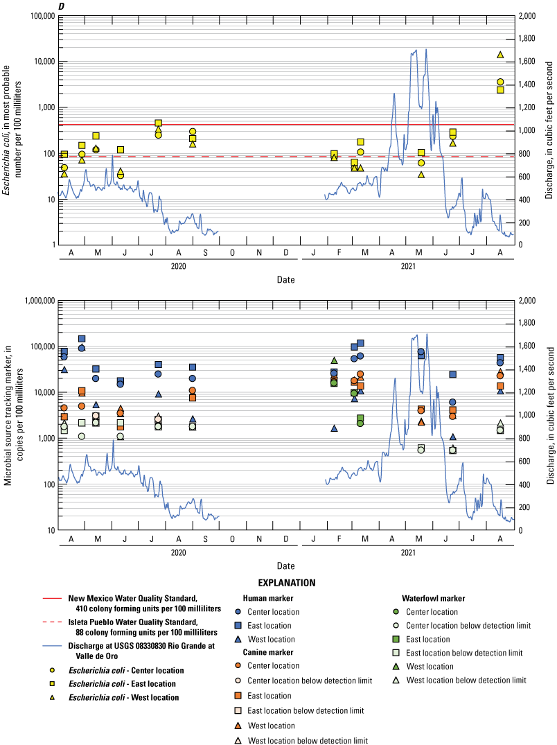
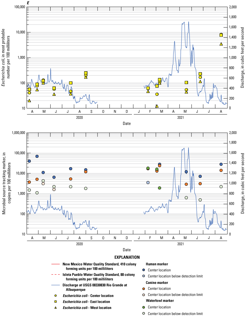
Escherichia coli and microbial source tracking marker time series plots showing data collected from all events at the A, Bridge Blvd, B, Rio Bravo, C, Above Tijeras, D, Below Tijeras, and E, Valle de Oro sites.
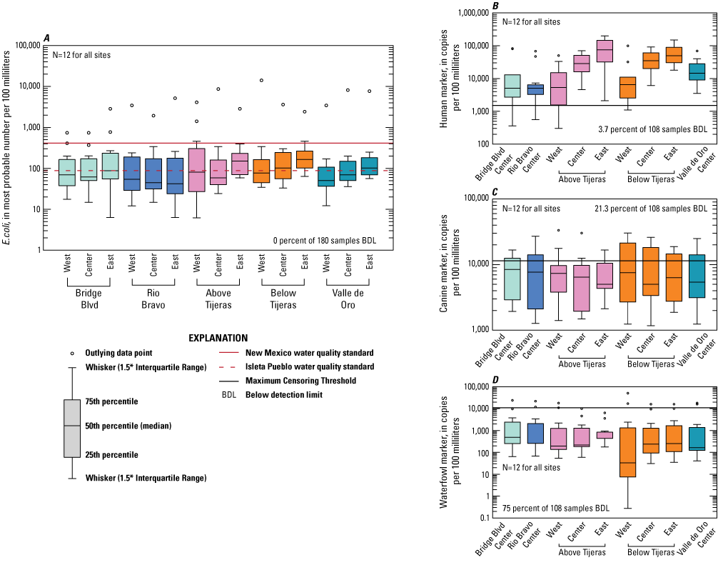
Escherichia coli (E. coli) and microbial source tracking marker boxplots showing data collected from all sampled events at five sites on the Rio Grande in Albuquerque, New Mexico.
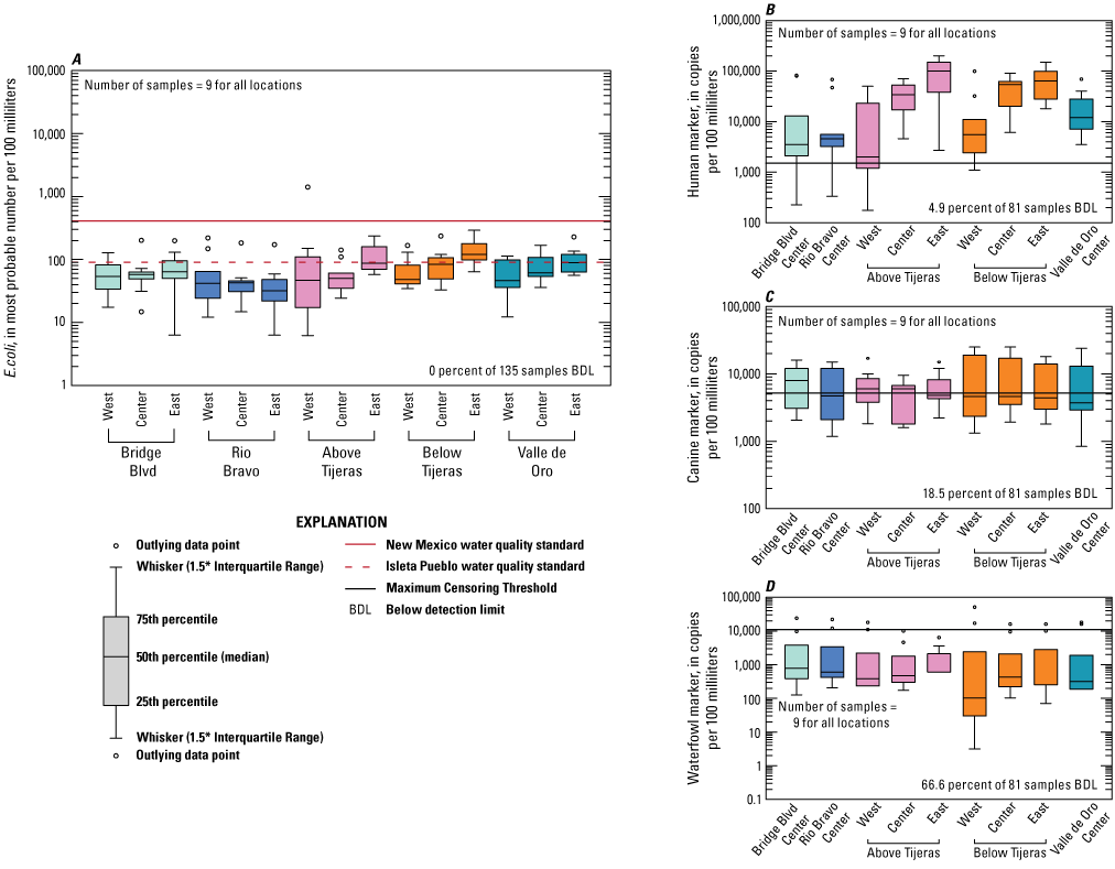
Escherichia coli (E. coli) and microbial source tracking marker boxplots showing data collected from dry season events at five sites on the Rio Grande in Albuquerque, New Mexico.
Correlation coefficients were computed to determine how well E. coli concentrations correlated with discharge, suspended sediment concentration, and turbidity (table 7). Relations between E. coli and the other constituents were not strong (Pearson’s r < 0.9 and Kendall’s tau < 0.7), which is likely because the majority of these samples were collected in the dry season, when E. coli concentrations aren’t likely to be due to increased flow, such as during storm events with greater discharge. The strongest correlation is between E. coli in water and turbidity.
Table 7.
Correlation statistics calculated for all data, including Escherichia coli (E. coli) in water and bed material against discharge, turbidity, and suspended sediment concentration.[NC, not calculated]
Escherichia coli Mean Daily Fluxes
Mean daily fluxes were calculated for each E. coli sample collected from the three-point sampling events (fig. 11, table 8). The TMDL for E. coli for the study reach ranges from 5.27 × 10¹² cfu/100 mL/day in high flow conditions (2,960 million gallons per day or 4,580 ft3/s) to 1.89 × 10¹¹ cfu/100 mL/day in low flow conditions (106 million gallons per day or 164 ft3/s; NMEDSWQB, 2019b). Because there were limited E. coli sampling data, true loads could not be calculated, and fluxes (MPN/day) are the rates that have been calculated. Therefore, the TMDL and the fluxes cannot be directly compared.
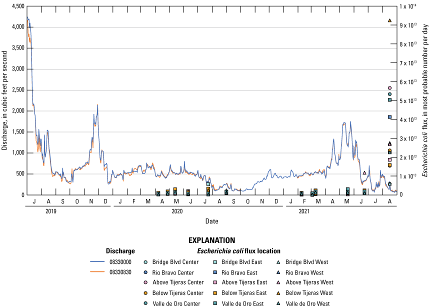
Mean daily fluxes for Escherichia coli and corresponding discharge during the study period.
Table 8.
Escherichia coli (E. coli) fluxes for each site and event at the three-point sampling locations.[Data from U.S. Geological Survey (USGS, 2021). Dates shown as month/day/year. Mean daily flux values are shown in E notation. MPN/d, most probable number per day; Blvd, boulevard]
Fluxes were consistently under 1.0 × 10⁴ billion MPN/day for the bulk of the study except for one event (fig. 11), which was a large storm event. That last storm event, which was in August 2021, had the greatest fluxes ranging from 5.89 × 10³ billion MPN/day to 9.25 × 10⁴ billion MPN/day.
Comparison of Escherichia coli to Water Quality Standards
Two water-quality standards were used for comparison to the data collected during this study. The NMWQS 20.6.4.105 and 20.6.4.900 New Mexico Administrative Code (New Mexico Water Quality Control Commission, 2010) for E. coli for a single sample is 410 cfu/100 mL for the study area reach. Additionally, Isleta Pueblo has a standard for E. coli for a single sample of 88 cfu/100 mL for primary contact ceremonial and recreational use. All sites and locations had E. coli concentrations exceeding both standards. In total, 72 samples exceeded the Isleta Pueblo standard of 88 cfu/100 mL, and 19 samples exceeded the NMWQS of 410 cfu/100 mL. In samples collected during only the dry season, 41 samples exceeded the Isleta Pueblo standard, and 1 sample exceeded the NMWQS.
Below Tijeras had the most exceedances with 11 sampling events having 1 or more sample locations exceeding the Isleta standard. Two events exceeded the NMWQS, both during the wet season. The exceedances ranged from 96 to 14,000 MPN/100 mL, and the east bank had the most frequent exceedances for all 11 sampling events. For the dry season samples, Above Tijeras was the site having the one sample exceeding the NMWQS, with a value of 1,400 MPN/100 mL, and the Below Tijeras remained the site with the highest number of exceedances over the Isleta Pueblo standard.
Characterization of Escherichia coli and Particle Size Analysis in Bed Material
Samples for bed material analyzed for E. coli and particle size analysis were only collected during the dry season. The mean values for E. coli at all the sites ranged from 0.5 to 10 MPN/gDW (Table 6). Unlike the dry-season E. coli concentrations in water where the maximum value was observed at the Above Tijeras West location, the maximum concentration for E. coli in bed material was observed at Above Tijeras East with 59 MPN/gDW. There is little variation of E. coli in bed material between the sites (fig. 12). Six percent of bed material samples were below the detection limit. Above Tijeras showed the most variation between the west and east locations.
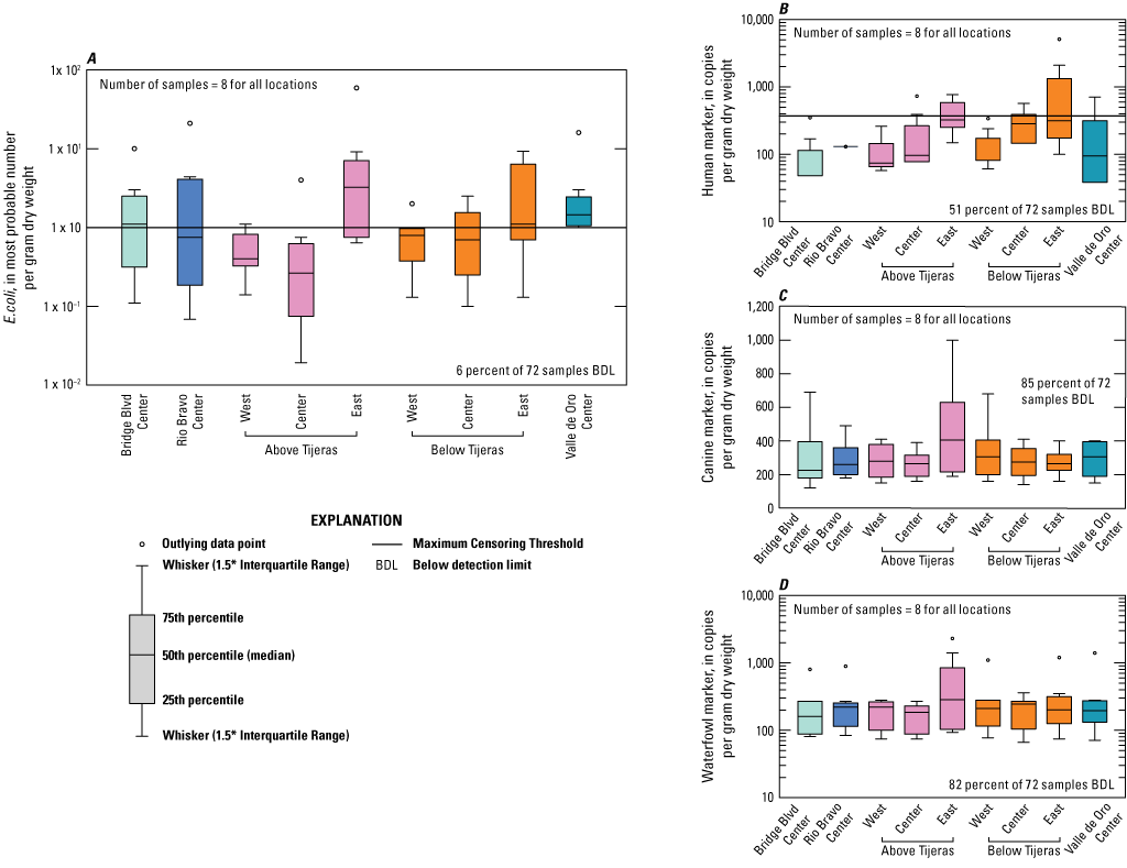
Escherichia coli (E. coli) and microbial source tracking markers in bed material boxplots showing data collected from all sampled events at five sites on the Rio Grande in Albuquerque, New Mexico.
Approximately 78 percent of the samples (n=72) had no fine particles (USGS, 2021). Bridge Blvd and Rio Bravo showed no fine material, but the downstream sites had a small percentage (4 percent or less) of fine material. Particle sizes in sediment have been identified as explaining some of the E. coli variability in rivers. Pachepsky and Shelton (2011) found more studies reporting an increase in E. coli concentrations when there was an increased amount of clay and silt bed material present. Coarse sediments may not provide as much protection from the sunlight or protozoan grazing for E. coli to survive as would finer sediments (Pachepsky and Shelton, 2011). Because E. coli concentrations in bed material were detected at low concentrations and the bed material is primarily a sandy substrate during the dry season, it is likely that the substrate is not a suitable habitat that would allow for bacterial growth during the dry season. Sampling particle size in both bed sediment and suspended sediment and E. coli concentrations in bed material during or directly after a storm would provide insight about whether more fine-grained material is present in bed material that could contribute to a higher E. coli concentration in the water.
This sand/fine particle ratio was compared to historical bed sediment data collected at the Albuquerque gage (USGS site no. 08330000) to understand if this finding is similar to historical data in the river. The gage is upstream from the sampling sites and was used for comparative purposes, because bed sediment used for particle-size analysis has been collected for more than 20 years and provides a good description of the bed particle size distribution. The bed sediment data collected from 2019 to 2020 (USGS, 2021) for 0.125-, 0.25-, 0.5-, 1-, 2-, 4-, and 8-mm particle size analysis were analyzed, and the first sediment particle size to reach 50 percent of the sample was considered the average size. For the entire date range, the average particle size during these years only ranged from 0.5 to 1 mm. As defined by the Wentworth Scale, 0.5 to 1 mm is considered “coarse sand” (Wentworth, 1922).
E. coli concentrations in bed material had little to no correlation between E. coli in water, turbidity, and suspended sediment concentration on the basis of Pearson’s r and (or) Kendall’s tau (table 7). Of the two, Kendall’s tau is a more appropriate indicator of correlation for these parameters because the relation between E. coli in bed material and E. coli in water, turbidity, and suspended sediment concentration is not linear. The highest correlation observed was between E. coli in bed material and E. coli in water, with a Kendall’s tau of 0.24; however, it is well below the value of 0.7 and so does not indicate a strong correlation.
Microbial Source Tracking in Water and Bed Material
The human marker was detected in all but 3.7 percent of the 108 water samples collected (figs. 8–10). The human marker concentrations in water vary by location, increasing downstream from the effluent outfall (observed mainly in center and east locations of the Above Tijeras and Below Tijeras sites) and do not vary by season. Median values in water samples ranged from 5,100 to 75,000 copies/100 mL for all data collected (fig. 9, table 9), and 2,000 to 100,000 copies/100 mL for concentrations during the dry season (fig. 10). The eastern sample location at Above Tijeras had the highest concentrations of up to 200,000 copies/100 mL, and that sample had a corresponding E. coli concentration in water of 160 MPN/100 mL.
Table 9.
Summary statistics for human microbial source tracking markers in water for all samples and dry season samples and bed material samples from the dry season.[Data from U.S. Geological Survey (USGS, 2021). copies/100 mL, most probable number per 100 milliliters; copies/gDW, copies per gram dry weight; Blvd, boulevard; <, less than]
No statistically significant correlation was found between E. coli concentrations in water and the human marker concentrations in water for this study, which was focused on dry season sampling (table 7). Although elevated human marker concentrations could indicate increases in fecal contamination, that was not observed during this sampling. The qPCR methods used in this study do not distinguish between viable and nonviable Bacteroides bacteria from which the human marker originates, and it has been found that dead bacteria can be detected by the method up to 4 weeks after it has been killed (Nielsen and others, 2007). Therefore, a high human marker concentration does not always equate with a high viable E. coli concentration, as was the case downstream from the effluent outfall, where a large amount of nonviable human-associated markers were found with smaller concentrations of E. coli.
For bed material samples, human marker median values ranged from 48 to 330 copies per gram dry weight (copies/gDW) (fig. 12, table 9). The maximum human marker observed in the bed material was 5,100 copies/gDW at Below Tijeras East, with an associated E. coli concentration of 4 MPN/gDW. There was also little correlation found between the E. coli concentrations in bed material and human markers in water (table 7).
The canine markers in water do not appear to vary by location and slightly decrease during the dry season (figs. 9 and 10; table 10). Of the 108 samples collected, 21.3 percent were below the detection limit. Median concentrations ranged from 4,800 to 7,400 copies/100 mL for all data collected (fig. 9) and ranged from 3,700 to 8,000 copies/100 mL during the dry season (fig. 10). The west sample locations at Above Tijeras and Below Tijeras had the highest concentrations (32,000 and 29,000 copies/100 mL, respectively) and corresponding E. coli concentrations of 4,100 and 14,000 MPN/100 mL, respectively.
Table 10.
Summary statistics for canine microbial source tracking markers in water for all samples and for samples collected during the dry season only.[Data from U.S. Geological Survey (USGS, 2021). copies/100 mL, most probable number per 100 milliliters; Blvd, boulevard;<, less than]
Summary statistics could not be calculated for the canine marker in bed material samples using the NADA package, because more than 80 percent of the data were censored (Lee, 2020). Maximum and minimum values in samples where the canine marker was above the detection limit were variable. The concentrations ranged from 180 to 680 copies/gDW. The maximum concentration of 680 copies/gDW was observed at Below Tijeras West and had a corresponding E. coli concentration in bed material of 0.9 MPN/gDW (USGS, 2021).
The waterfowl markers in water do not appear to vary by location and slightly increase during the dry season, during the months when the migratory bird population increases (figs. 8 and 9). Seventy-five percent of the 108 samples were below the detection limit. Median values ranged from 33 to 480 copies/100 mL for all data collected and increased to 100–780 copies/100 mL during the dry season (Table 11). The western sample locations at Below Tijeras had the highest concentration (51,000 copies/100 mL) and a corresponding E. coli concentration in water of 82 MPN/100 mL.
Table 11.
Summary statistics for waterfowl microbial source tracking markers in water for all samples and the samples collected during the dry season only.[Data from U.S. Geological Survey (USGS, 2021). copies/100 mL, most probable number per 100 milliliters; Blvd, boulevard; <, less than]
The waterfowl marker was not detected in 82 percent of bed material samples, and summary statistics could not be calculated using the NADA package (Lee, 2020). Maximum and minimum concentrations of the waterfowl marker that were above the detection limit were 1,100 and 130 copies/gDW, respectively. Out of this range, the maximum concentration was the only value reported that was not qualified as an estimate with “b” (extrapolated below the limit of quantification but above the limit of detection). This sample, having a concentration of 1,100 copies/gDW, was collected at the Below Tijeras site from the west bank location in February 2021 and had a corresponding E. coli concentration for this sample of 0.9 MPN/gDW (USGS, 2021).
Mean daily fluxes were calculated for each MST marker in water collected from the three-point sampling events (table 12). These fluxes were then ranked and placed in bins and those bins were used to compare fluxes of different microbiological constituents at a single site and across multiple sites. The flux ranks are discussed below, and scores were used to compare results across sites.
Table 12.
Microbial source tracking marker mean daily flux for each site and event at the three-point sampling location.[Dates shown as month/day/year. Mean daily flux values are shown in E notation. Blvd, boulevard; BDL, below detection limit]
Spatial and Temporal Evaluation
Data were evaluated to determine if there were any temporal (dry versus wet season) and spatial (sample site and location) differences using the Kruskal-Wallis and Peto-Peto test statistics (table 13). These statistical tests look for differences between centers of independent groups (Helsel, 2012;Helsel and others, 2020). The most notable seasonal differences were observed in E. coli concentrations in water, suspended sediment concentrations, dissolved oxygen, and turbidity, which is consistent with the wet season samples collected after storm events, which can contribute E. coli and sediment to the system. Seasonal variation was not evaluated in bed material because all bed material samples were collected in the dry season. When evaluating the most statistically significant differences between sampling locations (each three-point sampling location at a sample site was grouped and evaluated), specific conductance, pH, and the human marker had the most statistically significant differences, most likely caused by the influence of the effluent along the eastern bank of the river downstream from the effluent outfall (fig. 4).
Table 13.
Kruskal-Wallis and Peto-Peto statistical test results for temporal and spatial differences.[Statistically significant probability values (p-values; less than 0.05) are bolded. Small p-values are shown in E notation. E. coli, Escherichia coli; NC, not calculated]
The pH was significantly lower, and the specific conductance was significantly higher at several sites and locations downstream from the effluent outfall (fig. 6). The pH and specific conductance at Above Tijeras East were statistically significantly different from all of the other locations (pH p-values ranged from 0.0003 to 0.0128 and specific conductance p-values ranged from 0.0002 to 0.0078). This statistically significant difference continued downstream but began to dissipate through the cross sections at the Below Tijeras and Valle de Oro sites (fig. 6).
The human marker increases significantly at the effluent outfall (fig. 9). Above Tijeras East and Center differed significantly from the upstream sites and western sites downstream, with p-values ranging from 0.0051 to 0.0311. Although this difference was notable, there was no statistically significant increase of E. coli input into the system at the effluent outfall. As noted in the previous section, the analytical method does not distinguish between viable and nonviable bacteria (Nielsen and others, 2007). E. coli concentrations are a measurement of viable bacteria, but there was no statistically significant increase of E. coli concentrations in water noted throughout the study area since the study largely sampled during the dry season. Because the E. coli concentrations throughout the study reach did not have statistically significant differences, this would indicate that the effluent outfall was not a significant contribution of E. coli in the study area, and therefore the source of bacteria could be originating upstream from these sites.
The E. coli concentrations in bed material were statistically significantly greater at Above Tijeras East (p-values = 0.048), as compared to the other locations at Above Tijeras (fig. 12). The concentrations at Valle de Oro Center were significantly greater than those at the Above Tijeras Center and Above Tijeras West locations (p-values = 0.048) and those at Below Tijeras West (p-value = 0.048).
Strength of Bacteria and Potential Sources
Mean daily fluxes were calculated for E. coli and MST markers in water (tables 8 and 12). These fluxes were used to compare different microbiological constituents across multiple sites. The fluxes were ranked by site and placed into four equally sized bins with flux ranges for each bin listed in table 3 and the average bin scores listed in table 14 and figure 13. All results below the detection limit were placed into the 0 bin. The average bin scores listed in table 14 and illustrated in figure 13 can be used to compare the fluxes of a single constituent across sites and to compare the fluxes of different constituents at a single site.
Table 14.
Bin scores for Escherichia coli (E. coli) and microbial source tracking markers at all sites for all samples and dry season samples.[Blvd, boulevard]
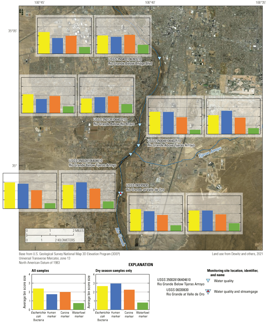
Average bin scores for Escherichia coli and microbial source tracking markers from all events and dry season events at five sites on the Rio Grande in Albuquerque, New Mexico.
The results of bin rankings indicate that for all samples, the E. coli mean daily fluxes were greatest at the Below Tijeras, Above Tijeras, and Valle de Oro sites (fig. 13). Average bin scores for the human marker were also highest at these sites (table 14), implying they are near a source of human fecal contamination. The average bin scores for the canine marker were highest at Bridge Blvd and Below Tijeras. Within each site and among the three MST markers, the canine marker had the highest bin score at Bridge Blvd and Rio Bravo, and the human marker had the highest bin score at Above Tijeras, Below Tijeras, and Valle de Oro. The waterfowl marker was detected less frequently than the human and canine markers during both seasons, and bins scores were lower for all samples and the dry season. During the dry season, the average bin scores for E. coli and the human markers were highest at the same sites as those for all samples. The canine markers had the highest bin scores at Bridge Blvd and Below Tijeras. The waterfowl marker was found more often during the dry season than the wet season, and bin scores were highest at Bridge Blvd and Rio Bravo. Within each site and among the three MST markers, the canine marker remained the highest bin score at Bridge Blvd and Rio Bravo, and the human marker had the highest bin score at Above Tijeras, Below Tijeras, and Valle de Oro.
The top potential sources of fecal bacteria are human and canine (table 15) based on a combination of known potential sources of fecal bacteria, percentage of detections of the source markers in both water and bed sediment samples, and analysis of the average bin scores for daily mean flux (table 15). Given that the analysis of known-source fecal sample from the wastewater influent from the WWTP resulted in detection of the canine marker in addition to the human marker, this could indicate that the canine marker could at least in part be from wastewater influence. This occurrence is not unexpected because fecal bacteria may be transferred between host species living in close contact (Field and Samadpour, 2007; Stewart and others, 2007; Roslev and Bukh, 2011). With the presence of many different potential sources (fig. 4), the high incidence of septic use (LaMotte, 2018) and general park and trail use (City of Albuquerque Parks and Recreation Department Open Space Division, 2014) may be nonpoint sources contributing to the reach during the dry season because there is little correlation between E. coli concentrations and discharge. Also, the lack of statistically significant spatial differences in E. coli concentrations between sampling locations may also indicate that there are no significant contributions of E. coli within the study area and contributions could be coming from one or more sources upstream from the study area.
Table 15.
Summary of potential sources, Escherichia coli (E. coli) and microbial source tracking marker data from water samples at each site and location, and top source ranking.[MPN/100 mL, most probable number per 100 milliliters; NS, not sampled; copies/100 mL, copies per 100 milliliters; Blvd, boulevard; %, percent]
Summary
The Rio Grande, in southern Albuquerque, New Mexico, is a Clean Water Act Section 303(d) Category 5 impaired reach for Escherichia coli (E. coli). The reach is 5 miles in length, extending from Tijeras Arroyo to the Isleta Pueblo boundary. An evaluation of E. coli and microbial source trackers (human-, canine-, and waterfowl-specific sources) was conducted by the U.S. Geological Survey to determine the extent and source of fecal bacteria within the impaired reach of the Rio Grande during the dry season (November through June) in 2020 and 2021.
Samples collected during both the dry season and the wet season provided data over a range of flow conditions and provide insight about the extent and source of fecal bacteria. Because fecal microorganisms may readily attach to sediments, riverbed material samples were also collected. During the dry season, E. coli concentrations in water were primarily detected below the New Mexico Surface Water Quality Standard of 410 colony forming units per 100 milliliters and mostly human and canine sources were detected. However, approximately 40 percent of the water samples exceeded the Isleta Pueblo water-quality standard of 88 colony forming units per 100 milliliters.
E. coli concentrations in bed material were detected at low concentrations, and the bed material was a sandy substrate with little fine-grained material, likely not providing a suitable habitat for bacteria growth. Mostly human markers were detected in the bed material, with over 80 percent of the canine and waterfowl markers being below the detection limits.
Statistically significant spatial and temporal differences were found in water-quality samples for E. coli (seasonal) and the human marker concentrations (downstream from potential sources). Specific conductance and pH also exhibited statistically significant differences downstream from the effluent outfall, indicating that the effluent travels alongside the eastern bank of the Rio Grande for some distance. Given the lack of correlation with discharge and the human marker being most prevalent in the study area, the source of E. coli in the dry season is likely a persistent nonpoint source, such as leaking septic systems or illegal dumping in the area. The lack of statistically significant spatial differences in E. coli concentrations between sampling locations may also indicate that there are no significant contributions of E. coli within the study area and that contributions could be originating upstream from the study area.
After calculating the mean daily fluxes, ranking them, and placing them into bins, the average bin scores were used to compare the fluxes of a single constituent across sites and to compare the fluxes of different constituents at a single site. Human and canine sources were the strongest signals observed in the study reach.
With the presence of so many nonpoint sources of fecal bacteria, leaking septic systems, illegal dumping, and general park and trail use may be contributing the most E. coli bacteria to the reach during the dry season. The results from this study will help decision makers determine the efficacy of their best management practices and guide new practices to improve water quality in the study reach.
Acknowledgments
The authors would like to acknowledge those who helped collect and analyze samples during the Covid-19 pandemic and its associated challenges at the New Mexico Water Science Center, Kim Beisner, Johanna Blake, Joe Beman, Rob Henrion, Elaiya Jurney, Natalia Montero, and Harold Nelson; and at the Ohio Water Microbiology Laboratory, Lauren Lynch. We’d like to thank Jeb Brown, a USGS hydrologist, for providing guidance in the sediment interpretation and analysis.
References Cited
Albuquerque Bernalillo County Water Utility Authority, 2023, Reclamation: Albuquerque Bernalillo County Water Utility Authority web page, accessed February 19, 2023, at https://www.abcwua.org/sewer-reclamation/.
American Society for Testing and Materials, 2019, Standard test methods for determining sediment concentration in water samples: American Society for Testing and Materials, D3977–97 (Reapproved 2019), accessed March 28, 2022, at https://compass.astm.org.
Bartolino, J.R., and Cole, J.C., 2002, Ground-water resources of the Middle Rio Grande Basin, New Mexico: U.S. Geological Survey Circular 1222, 132 p., accessed November 28, 2021, at https://doi.org/10.3133/cir1222.
Bernalillo County, 2022, Stormwater pollution: Bernalillo County web page, accessed April 2, 2022, at https://www.bernco.gov/public-works/public-works-services/water-wastewater-stormwater/stormwater/stormwater-pollution/.
Bosque Ecosystem Monitoring Program [BEMP], 2021, BEMPscience/bemp_data—BEMP Core Community Science Data—Riparian floodplain (ver. v1.0): Zenodo database, accessed December 7, 2021, at https://doi.org/10.5281/zenodo.3697197.
City of Albuquerque [COA], 2019, FY19 MS4 annual report—Microbial source tracking study: City of Albuquerque, p. 464–621, accessed November 30, 2021, at https://documents.cabq.gov/municipal-development/city-of-albuquerque-fy19-ms4-annual-report-nmr04A014.pdf.
City of Albuquerque Parks and Recreation Department Open Space Division, 2014, Resource management plan for Tijeras Arroyo Biological Zone: City of Albuquerque Parks and Recreation Department web page, accessed December 13, 2021, at https://www.cabq.gov/parksandrecreation/documents/r-82-resource-mgmt-plan-for-tijeras-arroyo-final.pdf.
Copeland, R.R., 1995, Albuquerque Arroyos sedimentation study—Numerical model investigation: U.S. Army Corps of Engineers, Albuquerque District, Technical Report HL–95–2, prepared by U.S. Army Corps of Engineers, Vicksburg, Miss., 156 p., accessed March 28, 2022, at https://apps.dtic.mil/sti/pdfs/ADA293372.pdf.
Dewitz, J., 2021, National Land Cover Database (NLCD) 2019 products (ver. 2.0, June 2021): U.S. Geological Survey database, accessed December 3, 2021, at https://doi.org/10.5066/P9KZCM54.
Fluke, J., 2018, Characterizing patterns in E. coli levels in Rio Grande River water and riverbed: Albuquerque, N. Mex., University of New Mexico Department of Civil Engineering, master’s thesis, 106 p. [Also available at https://digitalrepository.unm.edu/ce_etds/209.]
Fluke, J., González-Pinzón, R., and Thomson, B., 2019, Riverbed sediments control spatiotemporal variability of E. coli in a highly managed, arid river: Frontiers in Water, v. 1, article 4, p. 1–12, accessed April 1, 2022, at https://doi.org/10.3389/frwa.2019.00004.
Green, H.C., Haugland, R.A., Varma, M., Millen, H.T., Borchardt, M.A., Field, K.G., Walters, W.A., Knight, R., Sivaganesan, M., Kelty, C.A., and Shanks, O.C., 2014, Improved HF183 quantitative real-time PCR assay for characterization of human fecal pollution in ambient surface water samples: Applied and Environmental Microbiology, v. 80, no. 10, p. 3086–3094.
Guy, H., 1969, Laboratory theory and methods for sediment analysis: U.S. Geological Survey Techniques of Water-Resources Investigations, book 5, chap. C1, 64 p., accessed January 12, 2022, at https://pubs.usgs.gov/twri/twri5c1/.
Helsel, D.R., Hirsch, R.M., Ryberg, K.R., Archfield, S.A., and Gilroy, E.J., 2020, Statistical methods in water resources: U.S. Geological Survey Techniques and Methods, book 4, chap. A3, 458 p., accessed February 25, 2022, at https://doi.org/10.3133/tm4A3. [Supersedes USGS Techniques of Water-Resources Investigations, book 4, chap. A3, ver. 1.1.]
Herzenberg, K., 2018, Bird migration in New Mexico: New Mexico Museum of Natural History and Science web page, accessed November 28, 2021, at https://nmnaturalhistory.org/sites/default/files/documents/education/BosqueEdGuide/BEG_BirdMigration_ENGLISH_2018_0820_FINALv2.pdf.
Jian, X., Wolock, D., and Lins, H., 2008, WaterWatch—Maps, graphs, and tables of current, recent, and past streamflow conditions: U.S. Geological Survey Fact Sheet 2008–3031, 2 p. [Also available at https://doi.org/10.3133/fs20083031.]
Julian, P., and Helsel, D., 2021, Package ‘NADA2’—Data analysis for censored environmental data (ver. 1.0.1): Comprehensive R Archive Network software release, accessed February 2022 at https://cran.r-project.org/web/packages/NADA2.
Kildare, B.J., Leutenegger, C.M., McSwain, B.S., Bambic, D.G., Rajal, V.B., and Wuertz, S., 2007, 16S rRNA-based assays for quantitative detection of universal, human-, cow-, and dog-specific fecal Bacteroidales—A Bayesian approach: Water Research, v. 41, no. 16, p. 3701–3715. [Also available at https://doi.org/10.1016/j.watres.2007.06.037.]
LaMotte, A.E., 2018, Estimated nitrogen from septic for the conterminous United States, 2010 (SepN_CONUS_bg_2010): U.S. Geological Survey data release, accessed March 24, 2022, at https://doi.org/10.5066/P9QTGSI7.
Lee, L., 2020, Package ‘NADA’—Nondetects and data analysis for environmental data (ver. 1.6–1.1): Comprehensive R Archive Network software release, accessed February 2022 at https://cran.r-project.org/web/packages/NADA/NADA.pdf.
Meals, D.W., Richards, R.P., and Dressing, S.A., 2013, Pollutant load estimation for water quality monitoring projects—Tech Notes 8 (April 2013): U.S. Environmental Protection Agency, prepared by Tetra Tech, Inc., Fairfax, Va., 21 p., accessed September 3, 2019, at https://www.epa.gov/sites/default/files/2016-05/documents/tech_notes_8_dec_2013_load.pdf.
Mueller, D.K., Schertz, T.L., Martin, J.D., and Sandstrom, M.W., 2015, Design, analysis, and interpretation of field quality-control data for water-sampling projects: U.S. Geological Survey Techniques and Methods, book 4, chap. C4, 54 p., accessed December 3, 2021, at https://doi.org/10.3133/tm4C4.
Myers, D.N., Stoeckel, D.M., Bushon, R.N., Francy, D.S., and Brady, A.M.G., 2014, Fecal indicator bacteria (ver. 2.1): U.S. Geological Survey Techniques of Water-Resources Investigations, book 9, chap. A7, sec. 7.1, accessed December 6, 2021, at https://water.usgs.gov/owq/FieldManual/Chapter7/7.1.html.
National Water Quality Monitoring Council, 2021, Water quality portal: National Water Quality Monitoring Council database, accessed December 5, 2021, at https://www.waterqualitydata.us.
Natural Resources Conservation Service, 2002, Rio Grande-Albuquerque watershed (HUC8 13020203): U.S. Department of Agriculture, Natural Resources Conservation Service web page, accessed November 28, 2021, at https://www.nrcs.usda.gov/Internet/FSE_DOCUMENTS/nrcs144p2_068347.pdf.
New Mexico Environment Department Surface Water Quality Bureau [NMEDSWQB], 2019a, 2018–2020 Clean Water Act 303(d)/305(b) integrated report: New Mexico Environment Department web page, accessed May 3, 2019, at https://www.env.nm.gov/surface-water-quality/2018-2020-ir/.
New Mexico Environment Department Surface Water Quality Bureau [NMEDSWQB], 2019b, Total maximum daily loads: New Mexico Environment Department web page, accessed May 3, 2019, at https://www.env.nm.gov/surface-water-quality/tmdl/.
New Mexico Environment Department Surface Water Quality Bureau [NMEDSWQB], 2019c, NPDES permits: New Mexico Environment Department web page, accessed November 13, 2019, at https://www.env.nm.gov/surface-water-quality/npdes-permits/.
New Mexico Environment Department Surface Water Quality Bureau [NMEDSWQB], 2021, 2020–2022 Clean Water Act 303(d)/305(b) integrated report: New Mexico Environment Department web page, accessed November 22, 2021, at https://www.env.nm.gov/wp-content/uploads/sites/25/2018/03/EPA-approved-2020-IR_012221.pdf.
New Mexico Environment Department Surface Water Quality Bureau [NMEDSWQB], 2022a, Comprehensive assessment and listing methodology: New Mexico Environment Department web page, accessed May 3, 2022, at https://www.env.nm.gov/surface-water-quality/calm/.
New Mexico Environment Department Surface Water Quality Bureau [NMEDSWQB], 2022b, Bacteriological sampling and analysis standard operating procedure 9.1: New Mexico Environment Department web page, accessed August 30, 2022, at https://www.env.nm.gov/wp-content/uploads/sites/25/2017/06/9-1-Bacteriological-Sampling-20201117-approved.pdf.
Nielsen, K.M., Johnsen, P.J., Bensasson, D., and Daffonchio, D., 2007, Release and persistence of extracellular DNA in the environment: Environmental Biosafety Research, v. 6, no. 1–2, p. 37–53, accessed April 2, 2022, at https://doi.org/10.1051/ebr:2007031.
Noble, R.T., Leecaster, M.K., McGee, C.D., Weisberg, S.B., and Ritter, K., 2004, Comparison of bacterial indicator analysis methods in stormwater-affected coastal waters: Water Research, v. 38, no. 5, p. 1183–1188. [Also available at https://doi.org/10.1016/j.watres.2003.11.038.]
Pachepsky, Y.A., and Shelton, D.R., 2011, Escherichia coli and fecal coliforms in freshwater and estuarine sediments: Critical Reviews in Environmental Science and Technology, v. 41, no. 12, p. 1067–1110. [Also available at https://doi.org/10.1080/10643380903392718.]
Paretti, N.V., Coes, A.L., Kephart, C.M., and Mayo, J.P., 2018, Collection methods and quality assessment for Escherichia coli, water quality, and microbial source tracking data within Tumacácori National Historical Park and the upper Santa Cruz River, Arizona, 2015–16: U.S. Geological Survey Scientific Investigations Report 2017–5139, 30 p., accessed September 21, 2021, at https://doi.org/10.3133/sir20175139.
Paretti, N.V., Kephart, C.M., Porter, T.J., Hermosillo, E., Cederberg, J.R., Mayo, J.P., Gungle, B., Coes, A.L., Tucci, R.S., and Norman, L.M., 2019, Spatial and temporal distribution of bacterial indicators and microbial-source tracking within Tumacácori National Historical Park and the upper Santa Cruz River, southern Arizona and northern Mexico, 2015–2016: U.S. Geological Survey Scientific Investigations Report 2019–5108, 102 p., accessed September 21, 2021, at https://doi.org/10.3133/sir20195108.
Parsons Water & Infrastructure, Inc., 2005, Middle Rio Grande microbial source tracking assessment report: New Mexico Environment Department, Albuquerque Metropolitan Arroyo Flood Control Authority, Bernalillo County, prepared by Parsons Water & Infrastructure, Inc., Austin, Texas, 331 p., accessed May 5, 2022, at https://www.cabq.gov/municipaldevelopment/documents/storm-drainage-documents/storm-drainage-pdfs/MRG-MSTReport.pdf.
Pohlert, T., 2021, PMCMRplus—Calculate Pairwise Multiple Comparisons of Mean Rank sums extended: Comprehensive R Archive Network software release, accessed February 2022 at https://cran.r-project.org/web/packages/PMCMRplus.
R Core Team, 2022, R—A language and environment for statistical computing: Vienna, Austria, R Foundation for Statistical Computing website, accessed February 2022 at https://www.R-project.org/.
Rantz, S.E., and others, 1982, Measurement and computation of streamflow, volume 1—Measurement of stage and discharge: U.S. Geological Survey Water-Supply Paper 2175, 284 p., accessed December 16, 2017, at https://pubs.usgs.gov/wsp/wsp2175/.
Sanders, E.C., Yuan, Y., and Pitchford, A., 2013, Fecal coliform and E. coli concentrations in effluent-dominated streams of the Upper Santa Cruz Watershed: Water (Basel), v. 5, no. 1, p. 243–261, accessed September 21, 2021, at https://doi.org/10.3390/w5010243.
Standard Methods Committee of the American Public Health Association, American Water Works Association, and Water Environment Federation, 2022, 9223 Enzyme substrate coliform test, in, Lipps, W.C., Baxter, T.E., and Braun-Howland, E., eds., Standard methods for the examination of water and wastewater: Washington D.C., APHA Press, 4 p., accessed December 28, 2022, at https://doi.org/10.2105/SMWW.2882.194.
Stiles, J., 2006, Quality-assurance plan for the analysis of fluvial sediment by the U.S. Geological Survey New Mexico Water Science Center Sediment Laboratory: U.S. Geological Survey Open-File Report 2006–1333, 23 p., accessed May 5, 2022, at https://pubs.usgs.gov/of/2006/1333/report.pdf.
Sullivan, B.L., Wood, C.L., Iliff, M.J., Bonney, R.E., Fink, D., and Kelling, S., 2009, eBird—A citizen-based bird observation network in the biological sciences: Biological Conservation, v. 142, no. 10, p. 2282–2292. [Also available at https://doi.org/10.1016/j.biocon.2009.05.006.]
Thorn, C.R., McAda, D.P., and Kernodle, J.M., 1993, Geohydrologic framework and hydrologic conditions in the Albuquerque Basin, central New Mexico: U.S. Geological Survey Water-Resources Investigations Report93–4149, 106 p. [Also available at https://doi.org/10.3133/ wri934149.]
Travis, R.E., 2023, Fecal bacteria and microbial source tracking marker data in the Rio Grande, Albuquerque, New Mexico 2017-2020: U.S. Geological Survey data release, https://doi.org/10.5066/P9Q2ECYV.
Turnipseed, D.P., and Sauer, V.B., 2010, Discharge measurements at gaging stations: U.S. Geological Survey Techniques and Methods, book 3, chap. A8, 87 p., accessed December 16, 2017, at https://pubs.usgs.gov/tm/tm3-a8/.
U.S. Environmental Protection Agency [EPA], 2021a, Water quality standards regulations—Pueblo of Isleta: U.S. Environmental Protection Agency web page, accessed November 22, 2021, at https://www.epa.gov/wqs-tech/water-quality-standards-regulations-pueblo-isleta.
U.S. Environmental Protection Agency [EPA], 2021b, Indicators—Enterococci: U.S. Environmental Protection Agency web page, accessed November 28, 2021, at https://www.epa.gov/national-aquatic-resource-surveys/indicators-enterococci.
U.S. Environmental Protection Agency [EPA], 2022a, Overview of listing impaired waters under CWA section 303(d): U.S. Environmental Protection Agency web page, accessed May 2, 2022, at https://www.epa.gov/tmdl/overview-listing-impaired-waters-under-cwa-section-303d.
U.S. Environmental Protection Agency [EPA], 2022b, Clean Water Act section 303(d)—Impaired waters and total maximum daily loads (TMDLs): U.S. Environmental Protection Agency web page, accessed May 3, 2022, at https://www.epa.gov/tmdl.
U.S. Geological Survey [USGS], 2004, Cleaning of equipment for water sampling: U.S. Geological Survey Techniques of Water Resources Investigations, book 9, chap. A3, 68 p., accessed March 26, 2020, at https://pubs.water.usgs.gov/twri9A4/.
U.S. Geological Survey [USGS], 2021, USGS water data for the Nation: U.S. Geological Survey National Water Information System database, accessed November 28, 2021, at https://doi.org/10.5066/F7P55KJN.
U.S. Geological Survey [USGS], 2022a, Hydrologic unit maps: U.S. Geological Survey web page, accessed May 4, 2022, at https://water.usgs.gov/GIS/huc.html.
U.S. Geological Survey [USGS], 2022b, USGS water data for the Nation: U.S. Geological Survey National Water Information System database, accessed August 30, 2022, at https://doi.org/10.5066/F7P55KJN.
U.S. Geological Survey [USGS], [variously dated], National field manual for the collection of water-quality data: U.S. Geological Survey Techniques of Water-Resources Investigations, book 9, chaps. A1–A10, accessed December 6, 2021, at https://pubs.water.usgs.gov/twri9A.
Visit Albuquerque, 2021, Neighborhood guide—Barelas/South Valley: Visit Albuquerque web page, accessed November 28, 2021, at https://www.visitalbuquerque.org/about-abq/neighborhoods/south-valley/.
Conversion Factors
U.S. customary units to International System of Units
Temperature in degrees Celsius (°C) may be converted to degrees Fahrenheit (°F) as follows:
°F = (1.8 × °C) + 32.
Supplemental Information
Specific conductance is given in microsiemens per centimeter at 25 degrees Celsius (µS/cm at 25 °C).
Concentrations of chemical constituents in water are given in milligrams per liter (mg/L).
A water year is the period from October 1 to September 30 and is designated by the year in which the period ends.
Abbreviations
AU
assessment unit
BEMP
Bosque Ecosystem Monitoring Program
COA
City of Albuquerque
DNA
deoxyribonucleic acid
EPA
U.S. Environmental Protection Agency
HUC
hydrologic unit code
MST
microbial source tracking
NADA
Nondetects and Data Analysis (software package)
NMED
New Mexico Environment Department
NMEDSWQB
New Mexico Environment Department Surface Water Quality Bureau
NMWQS
New Mexico Water Quality Standard
NMWSC
New Mexico Water Science Center
OWML
Ohio Water Microbiology Laboratory
qPCR
quantitative polymerase chain reaction
RSD
relative standard deviation
SD
standard deviation
TMDL
total maximum daily load
USGS
U.S. Geological Survey
WWTP
wastewater treatment plant
For more information about this publication, contact
Director, New Mexico Water Science Center
U.S. Geological Survey
6700 Edith Blvd. NE
Albuquerque, NM 87113
For additional information, visit
https://www.usgs.gov/centers/nm-water
Publishing support provided by
Lafayette Publishing Service Center
Suggested Citation
Travis, R.E., Wilkins, K.L., and Kephart, C.M., 2023, Assessing Escherichia coli and microbial source tracking markers in the Rio Grande in the South Valley, Albuquerque, New Mexico, 2020–21: U.S. Geological Survey Scientific Investigations Report 2023–5019, 48 p., https://doi.org/10.3133/sir20235019.
ISSN: 2328-0328 (online)
Study Area
| Publication type | Report |
|---|---|
| Publication Subtype | USGS Numbered Series |
| Title | Assessing Escherichia coli and microbial source tracking markers in the Rio Grande in the South Valley, Albuquerque, New Mexico, 2020–21 |
| Series title | Scientific Investigations Report |
| Series number | 2023-5019 |
| DOI | 10.3133/sir20235019 |
| Year Published | 2023 |
| Language | English |
| Publisher | U.S. Geological Survey |
| Publisher location | Reston, VA |
| Contributing office(s) | New Mexico Water Science Center |
| Description | Report: viii, 48 p.; Data Release |
| Country | United States |
| State | New Mexico |
| City | Albuquerque |
| Other Geospatial | Rio Grande, South Valley |
| Online Only (Y/N) | Y |
| Google Analytic Metrics | Metrics page |