

Developing a Habitat Model To Support Management of Threatened Seabeach Amaranth (Amaranthus pumilus) at Assateague Island National Seashore, Maryland and Virginia
Links
- Document: Report (14.8 MB pdf) , HTML , XML
- Data Releases:
- USGS data release - Assateague Island seabeach amaranth survey data—2001 to 2018
- USGS data release - Seabeach amaranth presence-absence and barrier island geomorphology metrics as relates to shorebird habitat for Assateague Island National Seashore—2008, 2010, and 2014
- Download citation as: RIS | Dublin Core
Acknowledgments
This work was funded by a U.S. National Park Service Northeast Region Regional Block grant. We thank Bill Hulslander and Jonathan Chase of the Natural Resources Division of Assateague Island National Seashore for providing the impetus for this work. We would also like to thank Tami Pearl, also of the Natural Resources Division of Assateague Island National Seashore. This work grew out of a long-term collaboration to study Charadrius melodus (piping plover) breeding range habitat preferences wherein we are grateful to Sara Zeigler of the U.S. Geological Survey (USGS) and Anne Hecht of the U.S. Fish and Wildlife Service, among many collaborators from the piping plover conservation community, for sharing their perspectives on threatened species habitat. Emily Sturdivant, now at the Woodwell Climate Research Center, developed the data extraction code while working as a geographer for the USGS. Julia Heslin of the USGS executed the final data extraction. The efforts of Rachel Henderson, Travis Sterne, and Julia Heslin are also appreciated for coordinating the associated data releases and composing the metadata for this study. We thank Sara Zeigler and Chris Sherwood of the USGS for providing helpful reviews of this report.
Abstract
Amaranthus pumilus (seabeach amaranth) is a federally threatened plant species that has been the focus of restoration efforts at Assateague Island National Seashore (ASIS). Despite several years with strong population numbers prior to 2010, monitoring efforts have revealed a significant decline in the seabeach amaranth population since that time, the causes of which have been unclear. To examine potential causes for the population decreases, and to help inform management practices for the future, we first evaluated 20 years of plant population data and three seasons of physical landscape characteristics of seabeach amaranth sites spanning the period of decline to assess how these may have contributed to decreases in habitat. Plant population trends, grazing data, and precipitation data indicate the population declines coincided with severe storms and periods of drought. Furthermore, we found that plants tended to occur at sites on portions of ASIS that were lower elevation on narrower regions of the island than sites where plants were not observed. Secondly, using two different data sampling schemes, we developed Bayesian networks to calculate probabilities of habitat and evaluate the importance of different variables, particularly morphologic metrics, included in the Bayesian networks. Model analyses showed that variables capturing the presence of, and proximity to, the seed bank were important for accurate hindcasts, and that specific barrier-island morphologies tended to occur at sites where seabeach amaranth was observed. More specifically, favorable habitat sites tended to be those more likely to experience overwash during high-water events, consistent with the long-held observations that the plants tend to occur in disturbance-prone settings. Model outputs provide spatially explicit maps of relative habitat suitability and helped to identify high-priority areas for amaranth protection. The modeling effort may also assist in determining the management actions most likely to result in the preservation of a long-term sustainable population.
Introduction
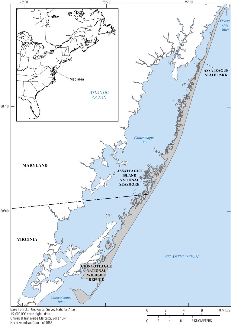
In April 1993, Amaranthus pumilus (seabeach amaranth, hereafter SBA), was added to the U.S. List of Endangered and Threatened Wildlife and Plants (U.S. Fish and Wildlife Service [USFWS], 1993, 2021). Historically, SBA occurred along the coast in nine States from Massachusetts to South Carolina (Weakley and others, 1996). The species inhabits sparsely vegetated upper beaches and washover terraces that are being reshaped continually by coastal processes. Since the conclusion of a restoration project in 2002, the National Park Service (NPS) has focused significant efforts on annually monitoring and managing the SBA population along Assateague Island National Seashore (ASIS; fig. 1). Despite several years of population increases, recent census data have revealed large annual variations and a steady decline in the ASIS SBA population during the last decade. In 2018, only four plants were detected during the annual census, compared to a high of more than 2,200 plants in 2007.
Map showing Assateague Island located along the mid-Atlantic coast of the United States.
Assateague Island is the only historically known Maryland site for SBA (Weakley and others, 1996; Tyndall and others, 2000) and is therefore an important location for conservation and long-term recovery for this species. Prior to 1998, when SBA was observed on Assateague Island there were few surveys of the island vegetation. The plant was recorded in the 20th century during a survey of the island flora in 1966 and 1967 (Higgins, 1969; Lea and others, 2003). This find represents the first record of SBA on Assateague Island in 31 years and the first recorded detection between North Carolina and New York in 26 years (Weakley and others, 1996). As SBA is an annual plant, reproduction and seed set within 1 year of growth are necessary to perpetuate populations. SBA possesses “fugitive species” adaptations (long-distance seed dispersal and long-lived seed banks) that allow it to opportunistically colonize new habitats as they develop following storm events (Weakley and others, 1996). The primary cause of the decline is believed to be development and stabilization of barrier-island beaches (Weakley and others, 1996). These processes reduce or eliminate natural disturbances that would otherwise create the overwash habitat required by the species. In some areas, recreational activities such as use of four-wheel-drive over-sand vehicles, intensive foot traffic, and beach grooming are thought to have caused population declines. Grazing along ASIS by ungulates (deer and horses) and insects also greatly reduces species survival and growth (Lea and others, 2003; Mark Sturm, National Park Service, written commun., 2007).
A large-scale restoration effort was undertaken at ASIS between 2000 and 2002 to re-establish the species (Lea and others, 2003). This was a cooperative effort involving multiple agencies (National Park Service, NPS; Maryland Department of Natural Resources, DNR; U.S. Fish and Wildlife Service, USFWS; and the Maryland Department of Agriculture, MDA) and numerous researchers (Lea and others, 2003; USFWS, 2006). Germplasm for the restoration was seed propagated from several plants found on the island, and the species was reintroduced during a 2-year period (fig. 2). A subsequent genetic variability study confirmed there were multiple genotypes present within the Assateague Island population and that restored individuals were not genetically identical (Hunter and others, 2001), suggesting there was sufficient diversity on the island to limit a potential genetic bottleneck.
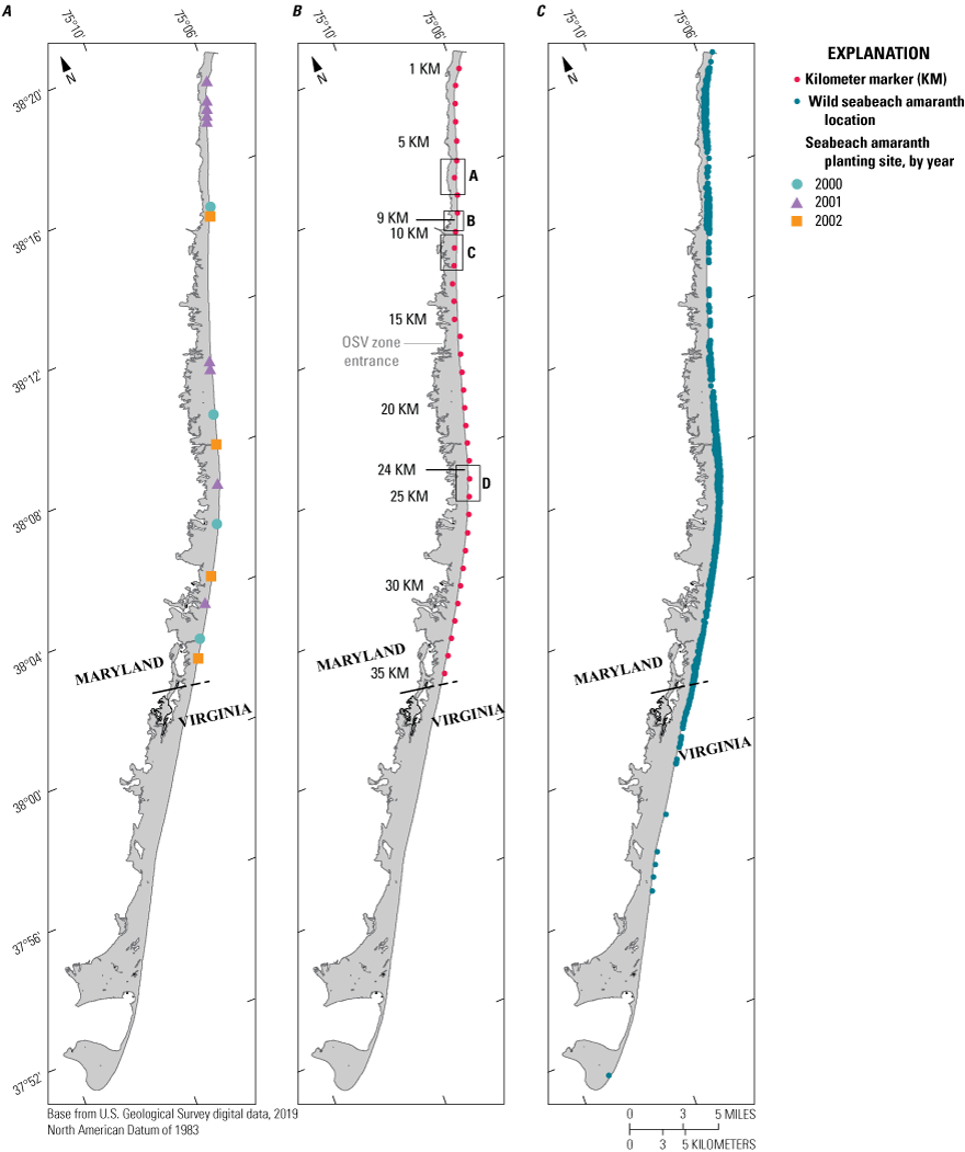
Maps of Assateague Island showing A, locations of seabeach amaranth planting sites and years planted, B, kilometer markers (KMs) used as reference locations, and C, the spatial distribution of wild seabeach amaranth plants from 2001 to 2018. The two regions of greatest seabeach amaranth abundance over the 18-year period are noted with black lines at 9 and 24 KM in map B. The gray line in map B between 16 and 17 KM indicates the northern extent of the over-sand vehicle (OSV) zone, and the inset boxes labelled with “A, B, C, D” specify regions shown in figures 12–15.
Despite the recognition of SBA as an important beach species, there have been few studies of its habitat preferences. Much of what has been written about SBA comes from the U.S. Fish and Wildlife Service recovery plan (Weakley and others, 1996). The only other study, Sellars and Jolls (2007), used SBA habitat characteristics on Core Banks, North Carolina. Their work relied on using remote-sensing data to develop a species distribution model informed with topographic characteristics sampled from digital imagery and light detection and ranging (lidar) data. They found that elevation was the most limiting factor for SBA with most occurring at elevations within 1.23 meters (m) of mean high water (MHW) and also in regions with little vegetation and near sites where plants had been present in previous seasons. In addition, they found that SBA did not occur in regions with strong erosional trends.
Despite the long history of monitoring at ASIS, the SBA population and the physical characteristics of where it occurs have not been studied in depth on the island. Although individual management actions have improved the probability of plant establishment and (or) growth, the relative efficacy of these efforts has yet to be evaluated. Also, the impact of individual management actions may depend upon location and the specific conditions of the year in which these actions were implemented. Because of this, NPS natural-resources staff at ASIS identified a need to conduct an in-depth evaluation of the SBA population data that have been collected since 2001 and develop a habitat model to evaluate SBA habitat suitability along ASIS. It is important to better understand SBA population variations over the last 20 years and how they may relate to barrier island morphological characteristics to better inform management efforts. Higher sea-level and more frequent and intense coastal storms due to future climate change will likely drive an increase in overwash events and create more open beach habitats along ASIS suitable to SBA. The potential effects to seashore infrastructure will require that both habitat and infrastructure needs be factored into long-term management practices. Consequently, developing a deeper understanding of the barrier island characteristics that constitute quality SBA habitat on Assateague Island can also inform future management efforts.
This report focuses on evaluating demographic and environmental monitoring data alongside physical observations of the coastal landscape to determine if there are unique physical characteristics that can describe SBA habitat and understand what may have contributed to SBA population decline. Our investigation first examines SBA population trends over a 20-year period during which SBA has been monitored at ASIS in comparison to meteorological factors. In addition, we examine the spatial distribution over this time period to determine if there are preferred settings where SBA tends to occur. While we focused on evaluating remote-sensing data sampling physical habitat characteristics, we also examined SBA population trends through comparison climatic factors such as precipitation and yearly observations of grazing to see if factors other than habitat descriptors influenced the plant population over time. Next, we evaluated physical habitat metrics using three datasets, for three different years—2008, 2010, and 2014—that capture a period when the population was relatively high (2008) and periods of decline (2010, 2014). We sampled remote sensing data via two sampling schemes to determine if there are unique characteristics where SBA tends to occur. In the last part of our analysis, we use these datasets to build probabilistic modeling frameworks, relying on Bayesian networks (BNs), to capture the essential physical barrier-island characteristics that describe suitable SBA habitat. The model framework is used to evaluate physical and environmental characteristics that occur in locations where SBA has been observed. We assess the sensitivity of predictions to different parameters in the model, which can in turn provide information to evaluate the relative importance of a variety of management actions for protecting SBA. Finally, we use prediction uncertainty to highlight knowledge gaps in our understanding of habitat preference, which can be used to guide future monitoring and management efforts.
A better physical understanding, based on the modeling parameters, of the landscape characteristics that the species prefers can help streamline monitoring efforts by allowing the most likely sites to be prioritized. This understanding can also improve management practices and increase the chance of establishing a viable SBA population on ASIS. Ultimately, the work described here is intended to provide information to support a better use of limited resources to protect the species. It also can be used to inform development of an adaptive management plan that is responsive to changing future conditions (Runge, 2011).
Setting
Assateague Island is a 60-kilometer (km)-long barrier island located along the mid-Atlantic coast of the United States. The island is oriented south-southwest, spanning the southern, ocean coast of Maryland and Virginia from Ocean City Inlet to Chincoteague Inlet (figs. 1 and 2). Assateague Island has a long history of episodic tidal inlets that form, exist for periods of a decade or more, and then close due to long-shore transport (Truitt, 1968; Dean and Perlin, 1977; Halsey, 1978; Oertel and Kraft, 1994; Krantz and others, 2009; Seminack and McBride, 2015). Before 1933, Assateague Island was part of a continuous barrier island called Fenwick Island that stretched north to the Maryland-Delaware border. In late August of 1933, the Chesapeake-Potomac Hurricane drove high water and wave conditions that breached Fenwick Island at the location of present-day Ocean City Inlet, the history of which is reviewed in Dean and Perlin (1977) and Krantz and others (2009). Following the breach, a decision was made to stabilize and maintain an inlet at Ocean City to improve Atlantic Ocean access for the town. The U.S. Army Corps of Engineers constructed a large jetty on the north side of the inlet to maintain the inlet opening and position. Within a year of construction, the jetty had formed a barrier to longshore sediment transport, depleting the sediment supply to northern Assateague Island. By 1935, a second jetty was constructed to stabilize the northern portion of Assateague Island adjacent to Ocean City Inlet. Since then, the northern 10 km of Assateague Island has eroded hundreds of meters landward requiring shoreline-change mitigation measures to maintain the barrier island and shoreline position (Dean and Perlin, 1977; Krantz and others, 2009).
A sustained management effort was undertaken in the early 2000s to address decades of sediment starvation resulting from the stabilization of the Ocean City Inlet (reviewed in Krantz and others, 2009; Schupp and others 2013). Extensive breaching of the island due to two strong nor’easters in February of 1998 resulted in the construction of an emergency berm along a 3-km section of the island’s northern section (fig. 3). This was followed by a large, one-time beach nourishment in 2002 along the northern 10 km of the island that emplaced 2.2 million cubic yards of sand. Since 2004, the island has undergone annual surf-zone sand emplacement of sands mined from the ebb tidal delta offshore of Ocean City Inlet as well as sand shoals that develop in the inlet channel. Due to these mitigation efforts, storm-driven overwash was less frequent along the managed area; however, NPS staff recognized that the lack of washover features had an impact on habitat quality for beach nesting shorebirds such as the Charadrius melodus (piping plover) (Schupp and others, 2013; Gieder and others, 2014). Consequently, passages to allow overwash during strong storms were constructed in 2008 (Schupp and others, 2013).
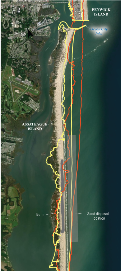
Aerial photograph showing the northern part of Assateague Island and southern part of Fenwick Island overlain by contours of shoreline position in 1850 and 1942, and the Ocean City Inlet that was created during a storm in August 1933 (data source: Maryland Geological Survey, 2006). Dark-gray shading specifies where a berm was constructed to reduce the likelihood of an unnatural breach forming after decades of sediment starvation. Light-gray area just offshore denotes the approximate region where ~46,000 cubic meters (60,000 cubic yards) of sand has been deposited twice per year after being dredged from the Ocean City Inlet and its ebb tidal delta. These actions have been undertaken since 2002 to restore the sediment supply to northern Assateague Island.
Since the initiation of the north-end restoration project in 2002, the SBA population along ASIS has been carefully monitored and actively managed on an annual basis to support population growth and demography. The result is over a decade of detailed census data on individual plant locations and size for reintroduced and wild plants, the latter being those that germinated from seeds in the environment. In addition, seed-bank dynamics, fecundity, seed dispersal, measures of habitat quality, and ungulate grazing impacts on survival and growth have all been studied in situ.
Methods
Analyses of SBA population trends and habitat metrics were conducted in three phases. The first phase focused on examining SBA population trends and their relation to meteorological trends and grazing as well as the spatial distribution of SBA on Assateague Island. The second phase focused on sampling presence-absence data and barrier island transect characteristics to determine if there were specific physical characteristics of SBA habitat. This in turn informed the development of BNs to model SBA habitat. The BN was used to evaluate the relative importance of each parameter in contributing to suitable habitat and refined to include those environmental characteristics found to be most important to the spatial distribution of SBA over time. These phases are described in the following sections.
Plant Census Data: Trends, Grazing, and Precipitation
Existing SBA census data for ASIS (collected by ASIS staff annually since 2001) were compiled to assist in developing the environmental variables for screening (Chase and others, 2023). These data consist of the measurement of plant geographic locations using a differential global positioning system (GPS) as well as descriptive observations of the approximate size and condition of the plants relative to whether they were grazed. In some cases, the density of SBA made it difficult to discern whether a single plant or multiple plants were present, so the number and approximate area observed may reflect the presence of multiple plants. For this reason, the number of observed plants in years of high plant abundance may be a minimum estimate of the plant population. Starting in 2005, the park staff noted whether plants were subject to grazing and, where possible, the grazing animal: wild horses, deer, or insects. Observers used the physical state of the plant to determine if insect or ungulate (deer and [or] horse) grazing had occurred. In addition, the ASIS natural resources staff reported whether plants were protected from horse or deer grazing by wire cages. Using these data, we explored spatial and temporal population trends and compared these against grazing observations and precipitation information (in other words, drought) to evaluate if these were factors that might further explain population declines. To determine if drought conditions coincided with the germination period of SBA, we compared the standardized precipitation index (SPI; Guttman, 1999; Keyantash and NCAR Staff, 2019; National Oceanic and Atmospheric Administration, 2020) to the number of plants observed for each year. In addition, we examined a newer but related index, the standardized precipitation evapotranspiration index (SPEI; Vincente-Serrano and others, 2010; Vincente-Serrano and National Center for Atmospheric Research Staff, 2015; Beguería and others, 2022). The SPEI incorporates estimates of potential evapotranspiration that take into account factors such as temperature and humidity. For both indices, we examined 1-, 3-, and 6-month time windows to verify the persistence of drought conditions at three time scales. For the analysis shown in this report, we use the 3-month time window.
Sampling Remote-Sensing Data
Because we relied on an existing monitoring dataset, we did not have the ability to design and execute a data-collection protocol; therefore, our initial phase required identifying datasets and conducting exploratory data analysis of metrics describing the physical environment during the 2001–20 time period. Although there have been a number of lidar surveys of Assateague Island, relatively few cover the entire island, and a number of these surveys followed severe coastal storms when island morphology differed from that present during the SBA growing season. Consequently, we selected three lidar datasets, two of which cover the entire subaerial extent of Assateague Island (2008, 2014) and one that covers mainly the ocean side of the island but was collected near a time when the island was surveyed for SBA (August 2010). Initially, our analysis focused on 2008 data (Bonisteel and others, 2009), due to prior experience using these data while investigating piping plover habitat (Gieder and others, 2014; Gutierrez and others, 2015). In addition, these data were acquired at a time when the SBA population count was relatively high and was not collected following a major storm. Data from 2010 (Bonisteel-Cormier and others, 2011) and 2014 (Sturdivant and others, 2019) were sampled when the population was substantially smaller. The 2010 lidar data did not cover the entire island, so the presence-absence points were confined to regions where lidar data measured island elevation. Lidar-derived metrics describing the physical setting from previously published datasets were sampled using two sampling strategies (Gutierrez and others, 2023). First, we followed previous species-distribution model research (Sellars and Jolls, 2007; Gieder and others, 2014; Zeigler and others, 2021) and sampled nine metrics (table 1) at point locations with plant-census data and at additional random point locations (Gutierrez and others, 2023). In years when there were more than 200 plant locations, an equal number of random locations were used. When plant numbers were below 100, we sampled three times that number of random point locations, following the example of Sellars and Jolls (2007), to attempt to sufficiently sample a range of settings on the island. Random point locations were generated using ArcGIS Pro ToolBox functions (ver. 2.0) via Python script that sampled points within the Assateague Island boundary, which comprises the mean-high water shoreline for the ocean side of the island and the mean tide level shoreline for the landward side (Gutierrez and others, 2023). Random points were spaced a minimum distance of 5 meters from other points (Gutierrez and others, 2023). Sampling of the 2010 dataset was limited to where lidar measurements were acquired on Assateague Island—generally consisting of the ocean-facing half to three-quarters of the barrier island. The nine characteristics were sampled from 5 x 5 m cells centered on each location (table 1). Six of the variables describe the position or physical state of the locations, as determined from the lidar data. One variable, vegetation type, describes the vegetative characteristics of a location, and the last two variables were proxies for SBA seed bank. The first of these, minimum distance to the nearest plant from the previous year, was motivated by the work of Sellars and Jolls (2007), who explored its efficacy as a seed-bank variable. We also tested a separate variable, number of plants within 30 m during the previous year, to also account for plant density. Vertical accuracies of the lidar were ±15 centimeters (cm) for 2008 and 2010 data and ±1 m for 2014.
Table 1.
Metrics recorded at each plant or random point location on Assateague Island.[Data source: Gutierrez and others (2023). MHW, mean high-water; m, meter; %, percent; NPS, National Park Service; ASIS, Assateague Island National Seashore; GPS, global positioning system; >, greater than]
| Metric | Description |
|---|---|
| Distance from the MHW shoreline (m) | The Euclidian distance between the center of the 5 x 5 m cell surrounding each point from the MHW shoreline on the ocean side of Assateague Island. The MHW shoreline was obtained from datasets compiled by Doran and others (2017); see also Gutierrez and others (2023). |
| Elevation (m) | The mean elevation of each 5 x 5 m cell surrounding each point relative to local MHW defined by Weber and others (2005) |
| Slope (%) | The mean slope of each 5 x 5 m cell surrounding each point |
| Aspect (degrees from north) | The compass orientation of the mean slope of each 5 x 5 m cell surrounding each point |
| Distance from nearest dune (m) | The Euclidean distance to the nearest foredune crest, as compiled by Doran and others (2017) and Gutierrez and others (2023) |
| Distance from nearest inlet (m) | The along-shoreline distance from Ocean City Inlet |
| Vegetation type | The density and type of vegetation present in a 5 x 5 m cell surrounding each point.
Vegetation-type shapefiles were created by the NPS staff at ASIS (NPS, 2008, 2010, 2014; Gutierrez and others, 2023). The shapefiles comprise plant vegetation type/density boundaries walked by NPS
staff using high-resolution GPS. Six classifications were specified: 1. Woody vegetation—specifies dominant cover being shrub or forest 2. Sparse vegetation—specifies lack of vegetation up to 20% cover by herbaceous vegetation 3. Herbaceous —specifies presence of herbaceous vegetation with >20% cover 4. Water—indicates presence of standing water (ponds) 5. Mud flat—indicates presence of muddy substrate lacking vegetation 6. Infrastructure—indicates presence of paved surfaces or buildingsa |
| Distance to nearest plant from the previous year (m) | The Euclidean distance of each point from the nearest plant observed in the previous year |
| Number of plants within 30 m from previous year | The number of plants encountered in a 30-m radius of each point |
Our second sampling strategy used measurements derived from lidar collected in 2008 and 2014 to sample metrics on barrier-island cross sections spaced every 50 meters (m) along the length of Assateague Island from Ocean City Inlet to Chincoteague Inlet (figs. 2 and 4; Gutierrez and others, 2023). The 2010 lidar dataset was not used because it did not cover the full width of Assateague Island, so it was not possible to sample some metrics, such as barrier width and mean elevation. The transects corresponded with those used to determine long-term shoreline-change rates (Himmelstoss and others, 2010). Eleven metrics were determined for each cross section (table 2).
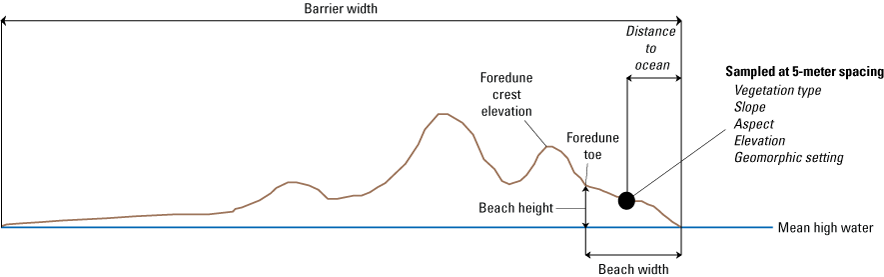
Schematic cross section illustrating the Assateague barrier-island metrics determined from existing light detection and ranging (lidar) and lidar-derived datasets. Metrics determined at plant and random-point locations are specified in italics. Metrics not in italics specify transect-based variables.
Table 2.
Barrier-island cross-section metrics sampled along 50-meter transects on Assateague Island.[Data source: Gutierrez and others (2023). m, meter; MHW, mean high water; m/yr, meter per year; %, percent; NOAA, National Oceanic and Atmospheric Administration; ND30, average number of plants within 30 meters of a transect from the previous year; D_trans, absolute value of the average distance of the transect to the nearest plant from the previous year]
| Metric | Description |
|---|---|
| Distance to the nearest tidal inlet (m) | The alongshore distance of each sampling transect intersects with the corresponding MHW shoreline for the sampling year (from Doran and others, 2017) |
| Long-term shoreline change rate (m/yr) | The long-term shoreline change rate determined by linear regression of 6–10 shoreline positions spanning a time period from 1845 to 2000 (Himmelstoss and others, 2010; Hapke and others, 2011) |
| Barrier width (m) | The horizontal distance between the transect intersections with the MHW position for a particular year, on the seaward facing shore, and the mean tide-level position on the landward facing shore (Sturdivant and others, 2019) |
| Mean transect elevation (m) | The average elevation sampled within 5-m bins sampled along each barrier-island transect. Mean barrier elevations were not calculated for transects having less than 20% missing values. In these cases, fill values were inserted. |
| Foredune crest height (m) | The elevation of the foredune crest relative to MHW as defined in Stockdon and others (2007, 2009, 2012). The dune height influences whether a barrier island is eroded, overwashed, or inundated by storm surge and wave runup position along a transect (Sallenger, 2000; Stockdon and others, 2007; Stockdon and others, 2012; Doran and others, 2017). Dune height elevations are referenced to local MHW (NOAA, 2018; Zeigler and others, 2019b) |
| Beach width (m) | The horizontal distance between the dune toe location (Stockdon and others, 2009; Doran and others, 2017) and the transect intersection with the MHW position for a particular year |
| Beach height (m) | The difference in elevation between the MHW shoreline (MHW=0) and the dune toe elevation |
| Human modificationsa | The presence of human modifications to Assateague Island. Six classifications were
applied: 1. Indicates the presence of no development, no nourishment, and no construction. 2. Indicates the presence of light development, no nourishment, and no construction. 3. Indicates the presence of moderate development, no nourishment, and no construction. 4. Indicates the presence of no development and either nourishment or construction. 5. Indicates the presence of light development and either nourishment or construction. 6. Indicates the presence of moderate development and either nourishment or construction. |
| Plant presence | Indicates that at least one plant was observed within 30 meters of a transect |
| Number of plants within 30 m from the previous year (ND30) | The average number of plants within 30 meters of a transect from the previous year |
| Distance to the nearest plant from the previous year (D_trans) (m) | The absolute value of the distance of the transect to the nearest plant from the previous year |
Field is the result of combining two definitions for human modification: “human_mod” and “human_modV2” in Gutierrez and others (2023).
Analyses of Sampled Data
Prior to development of the Bayesian networks (BNs), we conducted basic statistical analyses of the extracted metrics describing physical characteristics. First, bivariate Pearson correlation coefficients among sampled variables were calculated to identify variables that had high correlations. Those with high correlation were eliminated from the habitat models to minimize redundancies. Second, summary statistics for sampled variables (mean, standard deviation, and maxima and minima values) were used to determine if (a) there were distinct differences between locations/transects with observed plants and randomly selected locations, (b) transects where no plants were observed could help to identify preferred habitat characteristics spatially, and (c) whether changes in barrier-island morphology with time might correspond to changes in plant distribution. As part of this, we conducted t-tests to compare sample means between locations where SBA was and was not observed as well as Kolmogorov-Smirnov tests (Massey, 1951) to determine if samples had similarly shaped distributions.
Habitat Modeling Using Bayesian Networks
U.S. Geological Survey (USGS) and NPS collaborators worked together to develop Bayesian networks to serve as SBA habitat models. The BN is a predictive tool informed by observational data on both ecosystem response and external parameters that uses the relationships between them to make probabilistic predictions of a particular outcome—in this case, the probability of SBA presence. USGS collaborators have used this approach in coastal environments to predict the likelihood of change under various sea level rise (SLR) scenarios to evaluate piping plover habitat suitability (Gieder and others, 2014; Zeigler and others, 2019a and b), shoreline change, and barrier-island characteristics (Gutierrez and others, 2011, 2015; Fienen and others, 2013). We relied on the hypothesis that habitat suitability can be described, in terms of probability (P), as a function of physical conditions that were measured at locations where SBA plants have been observed. In the Bayesian framework this can be represented as
where the left hand-side is the conditional probability, S is suitable SBA habitat, the vertical line (|) indicates conditionality, f indicates a functional relationship, and the right-hand side of the equation is the prior (or existing) probability of the combined occurrence of the physical metrics. Equation 1 can be read as “the conditional probability of suitable habitat given the physical metrics of a location can be determined as a function of the combined likelihood of various physical aspects of the location in question.” The relationship represented in equation 1 can be cast in probabilistic form using Bayes’ theorem of conditional probability (Bayes, 1763), and Bayesian networks (BNs) provide ways to implement Bayes’ theorem. In Bayes’ theorem, one can compute the conditional probability of a given response (R) given the occurrence of some event (O):In equation 2, the left-hand side represents the conditional probability, also referred to as the posterior probability, of a particular response, Ri, given a set of observations (Oj) that are assumed to influence R. The subscripts i and j represent one of a finite set of scenarios that can be observed and the potential number of sets of observations, respectively. The numerator on the right-hand side contains two terms. The first is the likelihood of the observations if the response is known and indicates the strength of the correlation between observation and response. It is multiplied by the second term, which is the prior probability of the response, integrated over all expected observation scenarios. The denominator is a normalization factor that accounts for the likelihood of the observations.
Bayesian networks combine Bayes’ theorem with graphical models of a system, such as physical or biological systems (Pearl, 1978; Cowell, 1998; Heckerman, 1998; Jensen and Nielsen, 2007). We used the two sampling schemes to develop two types of BNs, one based on data associated with sample points where plants were observed (point model, PM) and one based on data associated with a transect across the barrier island (transect models, T). The two models rely on different data sampled at different resolutions, but both incorporate metrics describing the physical landscape where SBA was observed or was absent. For the point models, we assumed that the metrics associated with suitable SBA habitat were represented by the spatially averaged physical characteristics of a 5 x 5 m region surrounding points where plants were observed. For the transect models, we used a framework developed by Gutierrez and others (2015) in which physical characteristics were determined for barrier-island transects sampled every 50 m. The resulting BNs were constructed to predict the probability of seabeach amaranth presence on a transect. The BNs were developed using the Netica (version 5.24) software package by Norsys. BNs were trained with input data described previously using an expectation maximization algorithm to compute the posterior probability of each variable in question (Dempster and others, 1977; Lauritzen, 1995). Once the BNs were trained, data were processed using MATLAB-based computer codes like those developed using Python by Fienen and Plant (2015). These routines were also used to evaluate the BN datasets when used for hindcast skill testing and predictions.
We developed 24 versions of the point model BNs and 18 versions of the transect model BNs (tables 1.1 and 1.2, respectively). Each set of models used three different BN structures representing different assumptions and included different numbers of variables to test the impact of seed-bank variables on model results. The first, termed the simple BN structure, assumed that each variable had equal influence on SBA habitat suitability (figs. 5A and 5D). The second model, structured BN, included additional connections between variables that were thought to have an influence on one another (figs. 5B and 5E). The third model, TAN-structured BN, used a tree-augmented naïve Bayes (TAN) algorithm that can calculate the optimal BN structure (Friedman and others, 1997; Jiang and others, 2012; figs. 5C and 5F). This algorithm, implemented via Netica software, used a modified naive Bayes learning rule to evaluate the optimal BN structure for a specified dependent variable (Marcot and others, 2020). This is accomplished by identifying the dependent variable and linking variables according to their correlations. Links between covariates are possible if any covariates exhibit correlations after the most highly correlated variables are removed from the BN. The three model structures were used to compare models of differing complexity. As stated previously, the simple BN model assumes that each variable has an equal influence on habitat characteristics. The structured BNs incorporated connections between variables that were thought to have an influence on one another. In the case of the structured transect model (fig. 5E), this BN was based on one developed by Gutierrez and others (2015) that examined barrier island characteristics at Assateague Island. Last, the TAN-structured BNs represented optimized models that could be compared to determine potential outcome variability allowing for the training data to dictate model structure. By using three model structures, we were able to compare model results and show how differently structured models perform relative to one another. In this report we focus mainly on the results of the simple models (tables 3 and 4), but the full list of BNs and their performance assessment can be accessed in appendix 1.
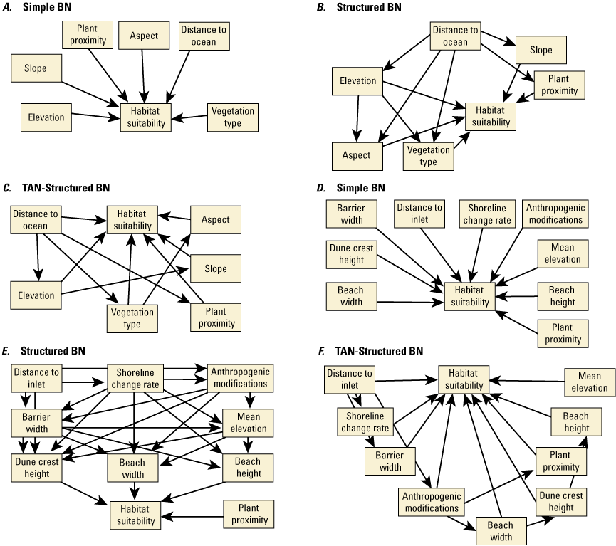
Schematic diagrams showing examples of the three main Bayesian network (BN) structures (simple, structured, and tree-augmented naïve Bayes [TAN]-structured) developed for the Assateague Island A–C, point and D–F, transect models. The plant proximity node specifies a node for distance to plants from the previous year or number of plants within 30 meters from the previous year. Tables 3, 4, 1.1, and 1.2 list all the variations of the six BN structures shown here.
Table 3.
Variables included in the point model Bayesian networks used as models of seabeach amaranth habitat on Assateague Island.[no., number; Dist. MHW, distance to the ocean-side mean high water shoreline; VT, vegetation type; ND30, number of plants within 30 meters of the location during the previous year; Dnp, distance to the nearest plant from the previous year; PM, point model; X (with shading), variable included in the BN; - (without shading), variable was not included]
Table 4.
Variables included in the transect model Bayesian networks used as models of seabeach amaranth habitat on Assateague Island.[no., number; Nour, nourishment; Const., construction; Devel., development; Dist., distance; ND30, number of plants within 30 meters of the location during the previous year; D-trans, distance to the nearest plant from the previous year; T, transect model; X (with shading), variable included in the BN; - (without shading), variable was not included]
For each of the three BN structures, several BNs were constructed using different combinations of input metrics. We used the correlation coefficients determined from the sampled data analysis to eliminate variables that were correlated from the BN. We also varied the number of variables in each model structure. This resulted in removing the vegetation-type variable and developing BNs with and without the seed-bank variables in the point models. Developing and evaluating BNs with differing structures and variables allowed us to develop reference comparisons for different BNs and understand the range of possible results. Our overall goal was to identify the best performing model and identify models that performed well with limited input variables. Appendix 1 provides a more comprehensive explanation of our experiments to identify the best performing models.
Model Evaluation: Scoring Metrics and Sensitivity Testing
We selected six BNs for fivefold calibration-validation testing (Fielding and Bell, 1997; Fienen and Plant, 2015) after evaluating the effect on model performance of different model structures and the inclusion of different numbers of variables (tables 2 and 3). For each BN, we randomly subsampled the datasets five times such that a fifth of the datasets were subsampled as a validation (or testing) set, and the remaining four-fifths of the datasets were retained as the calibration set (or training) set. Using each calibration set, we trained five implementations of each BN and computed calibration and validation performance scores.
The models were used to hindcast the probability of plant presence, and the hindcast outcomes were compared to the outcomes observed in the training data. The comparisons were used to calculate scoring metrics, two of which—error rate and false negatives and positives—we focus on in this report. The error rate is the percentage of outcomes in which the predicted outcome did not equal the observed outcome in the testing dataset. For the predicted outcomes, we defined probabilities as proportions where the probability of plant presence is P˃0.66 and P<0.66 to indicate plant absence. Error occurs when the BN-calculated posterior probability is P>0.66 but the corresponding observation indicates plant absence (in other words, a false positive) or a P<0.66 percent for a location where a plant was observed (in other words, a false negative). The threshold of 0.66 coincides with the Intergovernmental Panel on Climate Change (IPCC) definition for “likely” outcomes (Mastrandrea and others, 2010), as used in Zeigler and others (2019a, 2021). We report the percentage of erroneous predictions, partitioned as false positives and negatives. In some instances, we also specify where P>0.9 percent which coincides with the IPCC definition of “very likely.”
We also calculated spherical payoff and quadratic loss (Brier score), which are recommended metrics for models like BNs where the nuances of probabilities are an important consideration (Pearl, 1978; Morgan and Henrion, 1990; Marcot, 2012). Spherical payoff (SP) was calculated according to equation 3:
where MOAC refers to the mean probability of an outcome over all possible input cases with data, Pc is the predicted probability of the correct state, Pj is the predicted probability of state j, and n is the number of states. Scores vary between 0 to 1, with 1 indicating perfect model performance (Pearl, 1978; Morgan and Henrion, 1990; Marcot, 2012). Quadratic-loss (or the Brier score; QL) was calculated using the same variables as spherical payoff according to equation 4: Quadratic loss scores vary from 0 to 2, with 2 being a perfect model performance (Pearl, 1978; Morgan and Henrion, 1990). We also calculated Cohen’s Kappa to measure the agreement between the predicted and observed plant locations (Fielding and Bell, 1997). Kappa is where po is the observed agreement between raters and pe is the hypothetical probability of chance agreement. The terms po and pe can be calculated using confusion matrices, where po is: and pe is where a, b, c, and d represent the number of agreements (a and d) and disagreements (c and b) when predictions and outcomes are compared (table 5).[Symbols + and − represent example classifications of positive or negative. In this matrix, a and d represent agreements, and b and c represent disagreements]
We used a variance reduction scheme included with the Netica software (Fienen and others, 2013) to perform sensitivity tests to determine the influence of the input variables. Sensitivity was calculated according to equation 8 as the percentage of variance reduction (Vr) in a response variable after updating the finding for the input variable of interest:
where V(F) is the variance of a prediction before the update of an observed finding, and V(F|O) is the variance of the prediction after updating with the observations. V(F) and V(F|O) are calculated according to equations 9 and 10, respectively: where p(fj) is the prior probability of the jth prediction, fj is the actual value of the jth forecast, E(fj) is the expected value of the jth prediction (determined by the BN), p(fj|oi) is the updated (posterior) probability of the jth prediction given the ith evidence datum, E(fj|oi) is the expected value of the jth prediction given the ith evidence datum, M is the number of discrete evidence data, and N is the number of discrete predictions. The percent variance reduction is calculated as the variance calculated by using observations O from an input variable divided by the variance calculated by updating the response variable with findings of itself. Consequently, Vr for the prediction node is 100 percent while Vr for all other nodes is less than or equal to 100 percent. A Vr approaching 100 percent for a given node indicates that the BN output is sensitive to the value of that node. Conversely, a Vr approaching 0 percent indicates that the BN output is insensitive to the value of that variable.Results
Our results are organized into three parts. First, we examine the SBA population trends and the spatial distribution of plants on Assateague Island and relate them to observations of plant grazing and precipitation. Second, we analyze the morphological characteristics of SBA habitat from the remotely sampled data. Finally, we highlight the most successful BNs in modeling SBA habitat suitability.
Seabeach Amaranth Population Trends: 2001–20
Between 2001 and 2009, the SBA population consisted of 500 or more plants with numbers reaching almost a thousand individuals in 2001 and 2002 and exceeding 1,000 plants in 2006–9 (fig. 6). The peak occurred in 2007 with nearly 2,200 observed plants. The following year, the plant population decreased by over 50 percent to 1,048 plants. By 2010, the population had declined substantially to between 203 to 250 plants and declined to 8 plants in 2013. Since 2014, less than 50 plants have been observed each year except for 2015, when 122 plants were located. Only 4 plants were observed in 2018 and 2019, and no plants were found in 2020.
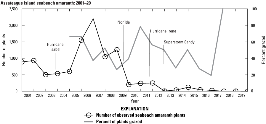
Numbers of observed seabeach amaranth plants from 2001 to 2020, Assateague Island. The timing of some of the large storms that affected Assateague Island is also shown.
SBA plants were spread predominantly along the northern ~40 km of Assateague Island. The northernmost plants occurred adjacent to Ocean City Inlet in 2002 and 2005. The southernmost plants were observed south of Toms Cove in 2004 nearly 25 km south of the southern-most planting area (see fig. 2), and only six plants were observed in the southern 17 km of Assateague Island between 2001 and 2005. Interestingly, the 2001 plants occurred nearly 13 km south of the southernmost 2000 planting area.
We examined the spatial and temporal distribution of SBA plants using the kilometer markers (KMs) provided by ASIS as spatial references (fig. 2; table 6). Plants were observed for at least 10 out of 20 years in KMs 9, 10, and 22–30 and only in KMs 9 and 10 after 2012. The greatest numbers of SBA plants were observed in KM 10 and KM 25, which contained 10 and 21 percent, respectively, of the total number of plants observed during the 20-year period.
Table 6.
Number of seabeach amaranth plants observed for each year in each kilometer zone, 2001–18, Assateague Island.[Data source: Chase and others (2023). See figure 2B for map showing the zones. No plants observed in 2019 or 2020. KM, kilometer marker; km, kilometer; %, percent; Tot., total; pop., population; npo, no plants observed]
Shaded cells specify the kilometer zone and year when plantings occurred (see fig. 2A for map). Shaded KM row numbers in the first column specify plantings in 2000 before annual census numbers were compiled.
There were a few regions in the Maryland portion of Assateague Island where plants were relatively sparse for the entire 20-year observation period. In the northern 20 kilometers, a rapid decline was observed from 2009 to 2012, and plants were only observed in KM 9 and KM 10 after 2012. In KMs 6–8, where a berm was put in place in 1999 to build up the barrier elevation and prevent an unnatural breach until the long-term sediment restoration program could be implemented (see fig. 3 and Morton and others, 2007; Krantz and others, 2009; Schupp and others, 2013), only 47 plants, less than 0.5 percent of the population, were observed. Ten plants or fewer were observed in KMs 1, 6, and 7.
Plant population declines were slower to the south. Here, low abundance coincided with Assateague State Park (KMs 11–15) and the beginning of over-sand vehicle (OSV) access (KMs 16–26). Assateague State Park is operated by the State of Maryland, and KMs 14–16 contain popular recreational beaches, campgrounds, and supporting infrastructure, such as parking lots and bathhouses. The infrastructure is protected by periodic dune maintenance to remediate erosion and to reduce the likelihood of overwash. During the 20-year observation period, 61 plants were observed between KMs 11–17 (0.6 percent of population) with none occurring at KM 13.
The spatial distribution of SBA varied during the period when we evaluated the models and their input data: 2008, 2010, and 2014. During 2008, observed SBA plants were widely distributed, extending from KM 1 just south of Ocean City Inlet to several km south of the Maryland-Virginia border, where 14 plants were identified (table 6). The highest plant density occurred in KM 25 (385 plants), followed by KMs 28 and 29 where 115 and 131 plants were observed, respectively. In 2010, plants were spread between KM 2 and KM 33 but concentrated in two main regions in KM 10, KM 24, and KM 25 with 120, 20, and 21 plants, respectively; this was after to a steep decline in KM 24 and KM 25 with 65 and 616 plants observed, respectively, in 2009. In 2014, plants occurred mainly in two regions, KM 10 and KMs 22–28 with counts of 2 and 37 in each, respectively. The highest number of plants occurred in KM 25 with 27 observed.
Population Trends and Grazing
Grazing by ungulates and insects was observed on many SBA plants. Figure 6 and table 7 display the number and percentage of plants where there was evidence that wildlife grazing occurred, where more than a third (mean of 39 percent) of plants showed evidence of grazing between 2005 and 2018. The number of plants affected by grazing ranged from 4 to 1,012, with the lowest (19 percent) and highest percentages (100 percent) occurring in years with small populations where 5 and 4 plants were observed, respectively. When the population exceeded 200 plants, the percentage of plants grazed ranged from 26 to 66 percent. In general, insect grazing was more prevalent, where on average, 39 percent of plants were grazed over the monitoring period; the maximum percentage that was subject to insect grazing occurred in 2011. Ungulate grazing was less prevalent, typically occurring on 10 percent of plants or less. On average, about 4 percent of plants were grazed by ungulates over the 13-year period.
Table 7.
Summary of the number of observed seabeach amaranth plants that were grazed from 2005 to 2018, Assateague Island.[Data source: Chase and others (2023). Ungulate grazing includes wild horse and deer. “Both” indicates evidence of grazing by insects and ungulates. Percentages are specified in parentheses. n, number; %, percent]
Population Trends and Drought
It has also been observed that early season conditions, such as drought, can have impacts on SBA. Weakley and others (1996, p. 1) suggested, based presumably on field observations, that SBA germinates as early as April and through at least July, and field observations on Assateague Island have been similar (B. Hulslander and J. Chase, NPS, oral commun., 2019). Typically, germination is observed in May and June, so we include April to examine if drought conditions occurred well before germination. It has been hypothesized that successful seed germination of SBA is more likely with warm, moist conditions during the late spring and early summer. Figure 7 shows the standardized precipitation index (SPI; Guttman, 1999; Keyantash and NCAR staff, 2019) and standardized precipitation-evapotranspiration index (SPEI; Vincente-Serrano and others, 2010; Beguería and others, 2022) plotted with the SBA population numbers. SPI is an established index to identify drought conditions, whereas SPEI is a more recent and more comprehensive index that factors in potential evapotranspiration and consequently considers the impact of temperature on water demand. The time series show that the SPI and SPEI indicate drought conditions during the typical germination time in three successive years: 2010, 2011, and 2012, indicated by the darker shaded areas in figure 7 that specify the April–July time window during which germination typically occurs. The drought conditions observed coincide with the decline in the SBA population post-2009.
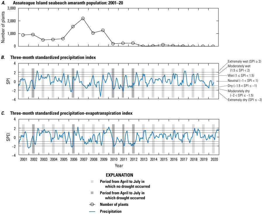
Graphs showing number of plants and precipitation data for Assateague Island from 2001 to 2020. A, Seabeach amaranth population, B, standardized precipitation index (SPI), and C, standardized precipitation evapotranspiration index (SPEI) for 3-month time scales. Negative values less than or equal to −1 indicate drought conditions. Light-gray shaded regions denote the April to July time period, toward the end of which seabeach amaranth germination typically occurs, where drought conditions did not occur. Darker gray shading indicates specific times when drought occurred in the April to July time period. >, greater than; <, less than.
Remote-Sensing Data: Statistical Comparisons and Correlations
We evaluated the characteristics of both observed plant point locations and transects affiliated with plant observations. Our data analysis focused on three questions:
-
Do the characteristics of locations and transects where plants were observed differ from characteristics of randomly selected locations (or transects) where plants were absent?
-
Do the characteristics of plant locations vary in time?
-
Are the physical characteristics of ASIS regions where plants were abundant (KMs 8–10 and KMs 24–25) different from those where plants were less abundant?
Characteristics of Observation and Random Point Locations
We found that the characteristics of observed SBA locations were distinct from random points in the 2008, 2010, and 2014 datasets (figs. 8 and 9; table 8). Comparison of 2008 point-location variables showed that statistically significant differences existed between observed locations and randomly selected locations (in both comparison of means via t-tests and comparisons of distributions via Kolmogorov-Smirnov tests; table 8). Observed plant locations generally occurred at higher elevations, closer to the shoreline, and in slightly steeper locations than random locations. Plant locations were also closer to the previous years’ plants (as noted by smaller distances to the nearest plants from the previous year, and the number of plants occurring within 30 m, table 8). Some characteristics of 2014 plant locations, including elevation, distance to the shoreline, and distance to the foredune crest, had similar values to the 2008 data. Plants occupied a similar elevation range (between 0.3 and 4.9 m), distance from the shoreline (120–123 m), and distance from the foredune crest (60–64 m). The rest of the 2014 variable means differed from 2008. However, the statistics for random points (which were more numerous than plant observations), were similar in 2014 and 2008. This indicates that most of the differences in means between the plant and random point locations were statistically significant (table 8). Exceptions occurred for slope (not significant at p=0.01) and distances to foredune crest and foredune toe (not significant at p=0.05). The 2010 plant location characteristics, while like those for 2008 and 2014, showed fewer differences between observation and random point locations. For 2010, differences in presence-absence data for elevation, distance to the shoreline and Ocean City Inlet, and distance to the nearest plant from the previous year were significant (table 8). On the other hand, aspect, slope, distances to dune positions, and the numbers of plants within 30 m did not illustrate significant differences when presence-absence characteristics were compared. When compared to 2008 and 2014, 2010 plant locations occupied similar elevation ranges and distances to the shoreline but occupied slightly higher elevation sites and were on average farther from the shoreline than the other two years.
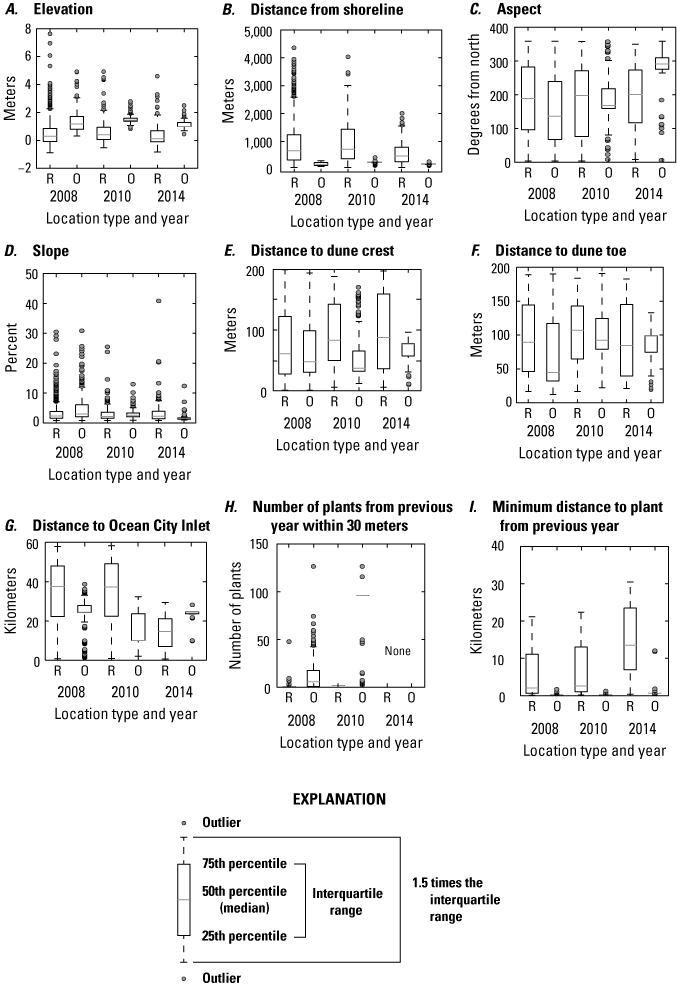
Boxplots summarizing 2008, 2010, and 2014 seabeach amaranth data, Assateague Island. A, Elevation, B, distance from shoreline, C, aspect, D, slope, E, distance to dune crest, F, distance to dune toe, G, distance to Ocean City Inlet, H, number of plants from the previous year within 30 meters, and I, distance to the nearest plant from the previous year. R indicates random locations, and O indicates locations where plants were observed.
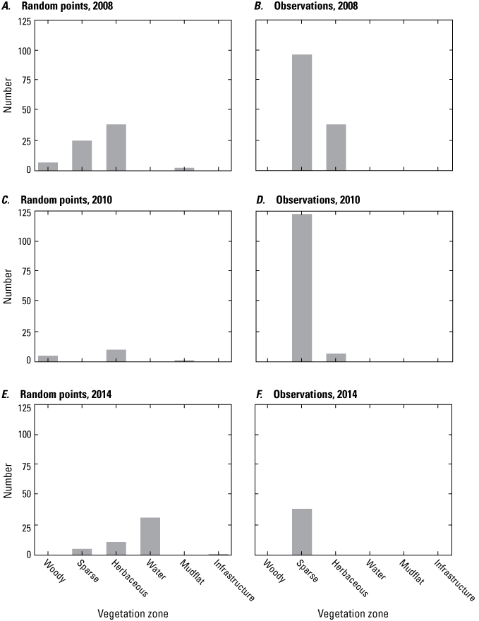
Histograms showing the distribution of vegetation zones on Assateague Island for random point locations (panels A, C, and E) and for locations where plants were observed (B, D, and F) in A, B, 2008, C, D, 2010, and E, F, 2014. The vertical axis is the number of data points in each vegetation zone. The number of data points, both plant and random point locations, occurring in regions where vegetation maps were available, were as follows: in 2008, 194 of 2,096; in 2010, 134 of 406; and in 2014, 39 of 156 (National Park Service, 2008, 2010, 2014; Gutierrez and others, 2023).
Table 8.
Statistics comparing observed seabeach amaranth locations with random point locations, 2008, 2010, and 2014, Assateague Island.[See footnotes for key to KS statistic column. Std. dev., standard deviation; Max, maximum; Min, minimum; KS, Kolmogorov-Smirnov statistic comparing values for observed seabeach amaranth locations (O) and values for random point locations (R); n/a, not applicable; Dist2 Shore, distance to shore; Dist DH, distance to the nearest dune crest; Dist DL, distance to the nearest dune toe; Dist 2 Inlet, distance to inlet; ND30, number of plants within 30 meters (m) of the location during the previous year; Dist 2, distance to; p = probability of obtaining the observed results assuming that the null hypothesis is true]
Figure 9 provides a summary of the vegetation categories that occurred at plant and random point locations coincident with available vegetation maps (NPS, 2008, 2010, 2014; Gutierrez and others, 2023). Overall, this information was available for less than 50 percent of both observation and random points for each year. Observed plant locations for each of the three years occur at sites that were classified mainly as sparse vegetation (<20-percent cover) with a smaller number classified as herbaceous vegetation (20–80-percent cover) and none occurring in other vegetation categories. In contrast, the random point locations for each year occurred in a wider range of vegetation categories.
Although correlation coefficients indicated weak to no correlation between most variables, several variable combinations did produce coefficients with magnitudes greater than or equal to 0.6 (table 9). Those found to be correlated included distance to MHW and foredune crest height, distance to MHW and foredune toe elevation, foredune crest height and foredune toe elevation, distance to Ocean City Inlet and vegetation type, and vegetation type and number of plants within 30 m from the previous year. As a result, foredune crest and dune-toe elevations, as well as distance to Ocean City Inlet, were not used in the SBA habitat models presented below. Despite the high correlation with distance to number of plants from the previous season, we retained vegetation type so we could test the habitat models and the impact of this variable when the seed-bank proxy variables were not available.
Table 9.
Correlation coefficients computed for observed seabeach amaranth locations with random point locations for Assateague Island 2008, 2010, and 2014 data.[Dist-Inlet, distance to inlet; DistMHW, distance to the ocean-side mean high water shoreline; distDH, distance to the nearest dune crest; distDL, distance to the nearest dune toe; VT, vegetation type; ND30, number of plants within 30 meters of the location during the previous year; Dnp, distance to the nearest plant from the previous year; ≥, greater than or equal to; p = probability of obtaining the observed results assuming that the null hypothesis is true]
Characteristics of Transects With and Without SBA
Comparison of metrics between transects where plants were present within 30 m and those where they were absent show that there were distinct characteristics at locations where SBA occurred in 2008 but not as consistently in 2014 (fig. 10; table 10). For 2008 data, we found statistically significant differences between transect metrics mean elevation, shoreline change rate, foredune crest height, beach height, and the seed-bank variables where plants were present and absent, both among their distributions (KS, table 10) and means (t-tests, table 10). The comparison of these metrics for 2008 indicated that SBA tended to occur in regions of Assateague Island with lower mean elevations, lower foredune crest elevations and lower beach heights. SBA also occurred on transects nearer to plants from the previous year. Also in 2008, SBA occurred on transects where higher rates of long-term shoreline erosion had been documented compared to transects where SBA was not present (table 10). In 2008, SBA also occurred on or near transects on narrower portions of Assateague Island and those having wider beach widths; however, differences in means for these variables were not statistically significant when transects without SBA nearby were randomly sampled from the dataset. Transect variable means for 2014 also differed for transects where SBA did and did not occur, but most of these differences are not statistically significant except for mean elevation and barrier width. In these cases, transects where SBA occurred had lower mean elevations and were located on narrower portions of Assateague Island.
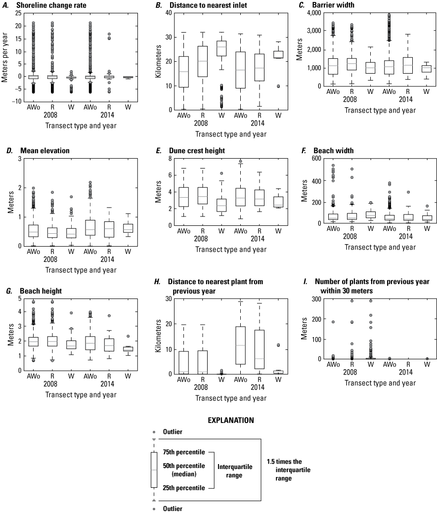
Boxplots summarizing 2008 and 2014 seabeach amaranth data, Assateague Island. A, Shoreline change rate, B, distance to nearest inlet, C, barrier width, D, mean elevation, E, dune crest height, F, beach width, G, beach height, H, distance to the nearest plant from the previous year, and I, number of plants from the previous year within 30 meters (m). AWo indicates all transects without seabeach amaranth (SBA) occurrences, R indicates randomly selected transects without SBA, and W indicates transects where plants were observed within 30 m of the transect.
Table 10.
Statistics for transects with seabeach amaranth, without seabeach amaranth, randomly sampled without seabeach amaranth, and transects from kilometer markers 9 and 25 where plants were abundant, 2008 and 2014, Assateague Island.[Randomly sampled transects without plants consisted of three-times the number of transects where plants were observed. Std. dev., standard deviation; Max, maximum; Min, minimum, KS, Kolmogorov-Smirnov; m/year, meter per year; w, transects with seabeach amaranth: number of observations (n)=196 for 2008 and n=12 for 2014; n/a, not applicable; w/o, transects without seabeach amaranth: n=975 for 2008 and n=1,194 for 2014; r-w/o, randomly sampled transects without seabeach amaranth: n=196 for 2008 and n=12 for 2014; KM 9 and KM 25, transects from kilometer markers 9 and 25: n=21; m, meter; p, probability of obtaining the observed results assuming that the null hypothesis is true]
We also compared the transect characteristics in regions KMs 9 and 25 (where SBA tended to be most abundant) with other transects to determine whether there were distinctions among the sites that might help to explain plant abundance (table 10). Both regions with abundant plants (KMs 9 and 25) tended to have narrower barrier-island widths, narrower beach widths, and lower beach heights than transects without plants and other transects with plants. There were differences between the two regions with abundant plants: KM 9 had a higher mean elevation and lower foredune crest elevation than other regions, and mean transect elevations were substantially lower for KM 25 than for all other regions, but the foredune crest elevations were similar to other regions.
To explore whether temporal changes in morphology may have been a factor in population declines, we compared morphological characteristics of Assateague Island and SBA habitat in 2008 and 2014, which were years of relatively high and low populations, respectively (where data measuring Assateague Island were available). Metrics for mean elevation, foredune crest height, beach width, and beach height were compared for three groups of transects (table 11). Group A lists all transect metrics in 2008 and 2014, group B lists metrics for transects where SBA was present in 2008 and 2014, and group C lists metrics for transects where plants were observed only in 2008 using data from both 2008 and 2014. Results show that, overall, the means of each variable were significantly different between the two periods (table 11). Mean elevations and foredune crests were higher in 2014, and beach elevations were lower and beach widths were narrower in 2014. The largest differences occurred for mean transect elevation and beach width; transects in 2008 had significantly lower mean elevations and wider beach widths compared to those in 2014 (see shaded region in table 11, group A). This contrasts with areas where plants were observed during both periods, where these metrics did not differ significantly (table 11, group B). However, when comparing transects where plants were observed in 2008 but not in 2014, foredune crest height, beach width, and beach height all differed between 2008 and 2014 (see shaded region in table 11, group C). In these cases, mean foredune crest height was nearly a meter higher in 2014 than in 2008. These comparisons show that barrier-island morphology changed between the 2008 and 2014 datasets, but suitable habitat characteristics remained unchanged.
Table 11.
Comparison of 2008 and 2014 morphological metrics for the entire Assateague barrier island and for locations where seabeach amaranth was present in 2008.[Note: there were no exact transects in common between 2008 and 2014. Shaded regions indicate specific results that are discussed in the text: beach width and beach height in table parts A and C and foredune crest height in part C. Std. dev., standard deviation; Max., maximum; Min., minimum; KS, Kolmogorov-Smirnov]
Examination of correlation coefficients revealed that only three sets of metrics showed moderate correlation, while the rest showed weak or no correlation (table 12). The three correlated pairs of metrics (correlation coefficient > 0.6)—distance to inlet and mean cross-section elevation; maximum elevation and foredune crest height; and foredune crest height and beach height—were not included in the SBA habitat models described in the next section.
Table 12.
Correlation coefficients for Assateague barrier-island transect metrics from 2008 and 2014.[SLC, shoreline change; WL, barrier width; MeanZ, mean transect elevation; MaxZ, maximum transect elevation; DHZ, foredune crest elevation; BW, beach width; BH, beach height; DIN, distance to nearest inlet; Nd30, number of plants within 30 meters (m) from the previous year; D_trans, distance to nearest plant from the previous year]
Bayesian Network Modeling
Point Model Cross Validation and Sensitivity
We constructed 24 BNs using point metrics. In this section, we focus on six of these BNs listed in table 3 (PM1–PM6). The full set of BNs is presented in appendix 1, section 1.2. The performance scores for each of the six BNs are listed in table 13. Overall, the simple and TAN BNs produced similar, and in some cases identical, performance scores and outperformed the structured BNs (app. 1). We evaluated the performance of six variations of the simple BNs using k-fold cross validation (see appendix 1), using fivefold calibration-validation testing. Results showed performance decreased for validation tests compared to calibration tests (table 13). The range of calibration test error rates were 2.1 percent for PM3 to 7.7 percent with PM6, and validation scores ranged from 12.7 percent for PM3 to 16.2 for PM1. Kappa values ranged from good (0.84 and 0.96) for calibration tests, to moderate (0.65 and 0.78) for validation tests. The highest performing BN was PM3, which included the seed-bank variable distance to the nearest 2007 plant. PM1, PM3, and PM5, which included the vegetation type variable, had higher performance scores compared to the versions of these BNs that did not include this variable (PM2, PM4, and PM6).
Table 13.
Performance metrics for fivefold cross-validation using Bayesian network point model data for Assateague Island.[See appendix 1, section 1.2, for additional performance results for all Bayesian networks tested in this study. PM1 includes variables: elevation, aspect, slope, distance to mean high water (MHW) shoreline, vegetation type and number of plants within 30 meters from the previous year; PM2 includes: elevation, aspect, slope, distance to MHW shoreline, and number of plants within 30 meters from the previous year; PM3 includes: elevation, aspect, slope, distance to MHW shoreline, vegetation type and distance to nearest plant from the previous year; PM4 includes: elevation, aspect, slope, distance to MHW shoreline, and distance to nearest plant from the previous year; PM5 includes: elevation, aspect, slope, distance to MHW shoreline, and vegetation type; PM6 includes: elevation, aspect, slope, and distance to MHW shoreline. BN, Bayesian network; no., number; PM, point model; Cal., calibration; Val., validation]
Figure 11 shows the percent variance reduction for four point BNs that we compared to examine the relative influence of different variables on them (in other words, sensitivity analysis). In addition to PM3 and PM4, we included PM1 and PM6 in this evaluation because they include different numbers of variables. PM1 includes the seed-bank proxy—number of plants within 30 m—from the previous year, and PM6 consists of morphological variables only. Consistent with the model performance results above, seed-bank proxy metrics had the largest influence on PM3 and PM4, followed by distance to the ocean shoreline (fig. 11A and B); additionally, the removal of vegetation type did not have a large effect on the relative influence of other variables on plant presence (fig. 11B). In figure 11C, when the number of plants within 30 m was included instead of the minimum distance to 2007 plants, the influence of distance to the ocean shoreline increased relative to the first few cases. In the last case, when the plant presence variables were not included, distance to the ocean shoreline had the largest influence in the BN, followed by elevation (fig. 11D).
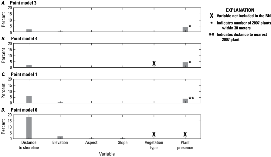
Graphs showing the percent variance reduction for each variable included in four different Bayesian networks (BNs) used as models of seabeach amaranth habitat on Assateague Island: A, point model 3, B, point model 4, C, point model 1, and D, point model 6.
Point Model Hindcasts
To further evaluate hindcast capability, we also compared the percentage of suitable habitat hindcast for KM zones where SBA was abundant with those where SBA was not observed during the 20-year time period with the six variations of the simple BN (table 13). Results for these comparisons are listed in table 14. Figures 12 through 14 show hindcasts for four locations conducted with four of these BNs.
Table 14.
Percent habitat hindcast for two sections of Assateague Island: kilometer marker (KM) 12 (State park) using the point model, where seabeach amaranth has not been observed, and KMs 24–25 where it has been abundant.[Numbers are percentages where P(Habitat) > 0.66 / P(Habitat) > 0.9. See appendix 1, section 1.2, for the full range of hindcast results with all Bayesian networks (BNs) investigated. P, probability; >, greater than; KM, kilometer marker; PM, point model]
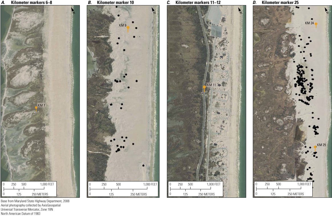
Aerial photographs from 2008 showing locations of the example model hindcasts and forecasts presented in the “Point Model Hindcasts” section of this report. A, Kilometer markers (KMs) 6 to 8, B, KM 10, C, KMs 11 and 12, and D, KM 25. Black dots denote the locations of observed seabeach amaranth plants in August 2008. Orange markers show the locations of KMs. See figure 2 for the location of each photograph on Assateague Island.
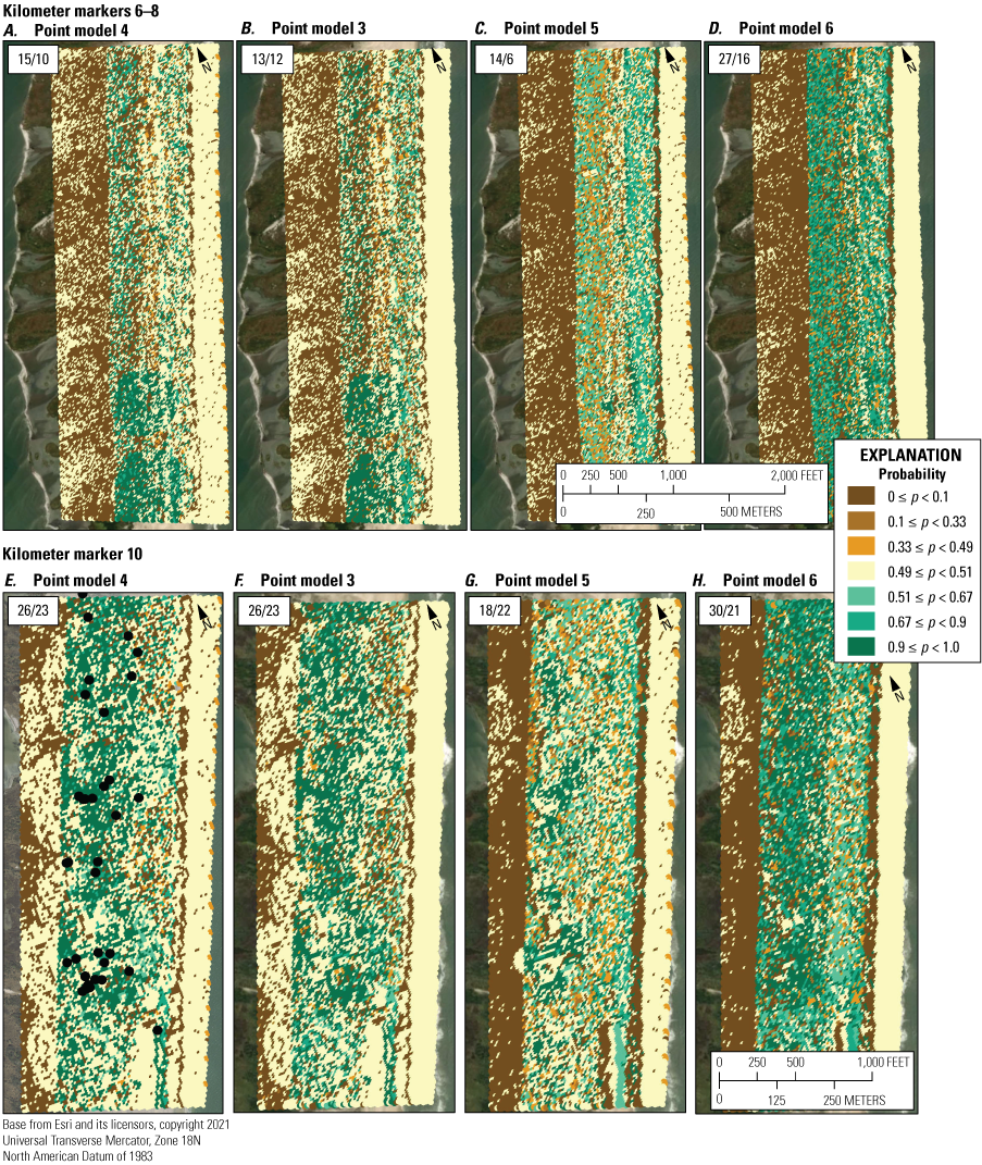
Hindcast point model results showing the habitat suitability probabilities for seabeach amaranth along A–D, kilometer markers (KMs) 6 to 8 and E–H, KM 10 on Assateague Island. Inset boxes at the upper left of each panel display the percentage of habitat probabilities greater than (>) 0.66 and >0.9. Black dots in panel E (lower left) show locations of observed seabeach amaranth plants in 2008. There were no plants present along KMs 6–8 during this time. See figures 2 and 12 for the location and aerial photographs of this region.
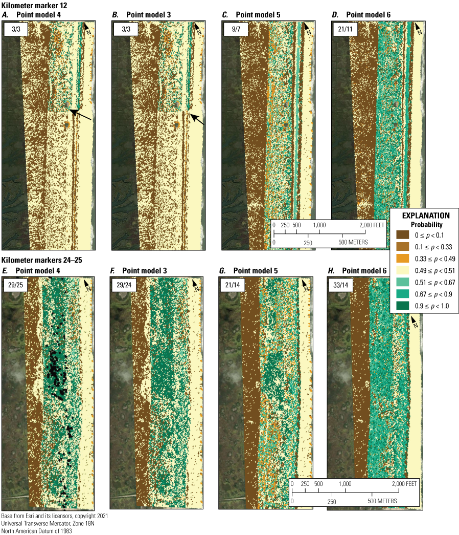
Hindcast point model results showing the habitat suitability probabilities for seabeach amaranth along A–D, kilometer marker (KM) 12 and E–H, KMs 24–25 on Assateague Island. Inset boxes at the upper left of each panel display the percentage of habitat probabilities greater than (>) 0.66 and >0.9. Arrows in top row denote a sharp transition in habitat probability for this region. Black dots in panel E (lower left) show the location of observed seabeach amaranth plants in 2008. There were no plants present for KM 12 during this time. See figures 2 and 12 for the location and aerial photographs of this region.
Overall, point models that included seed-bank proxy variables (PMs 1–4, number of plants within 30 m from the previous season, and distance to nearest plant from the previous season) were the best performing BNs with the lowest error rates and highest Kappa scores, spherical payoff, and quadratic loss scores (table 13). These models also correctly hindcast fewer sites with habitat and demonstrated more accurate hindcasts reflecting the presence or absence of SBA from a particular region (table 14; figs. 13A, B, E, F and 14A, B, E, F). When the seed-bank proxy variables were not included (PMs 5 and 6), the error rates were two-to-three times higher, the remaining performance metrics were lower (table 11), and the presence of habitat was overpredicted (table 14; figs. 13C, D, G, H and 14C, D, G, H). Specifically, where plants were not observed, PM6, which consisted of morphological variables only, hindcast the largest percentage of habitat (the majority of which were P<0.9; figs. 13D, H and 14D, H) and the greatest percentage of habitat with probabilities >0.9.
Performance scores for BNs were slightly better when vegetation type was included (table 13). Furthermore, the inclusion of vegetation type had greater impact on hindcasts from BNs that did not include a seed-bank variable (PM5 and PM6) versus those that did (PM3 and PM4). Specifically, the inclusion of vegetation type (PM3, figs. 13B, F and 14B, F) produced slightly less habitat where P>0.66 but slightly more where P>0.9 compared to the PM4 results. It is interesting to note that even without the seed-bank variables, hindcasts for KMs 24–25 using PM5 were more like PM4 than PM6 with the inclusion of the vegetation type variable (fig. 13). This shows that vegetation type may be a useful determinant for identifying habitat when seed-bank variables are not available.
Differences from the BN hindcast models were most apparent for KMs 11–13 (fig. 14A–D). In this region, PM3 and PM4 hindcast relatively little habitat, which is consistent with the absence of SBA in this region, both in 2008 and throughout the two-decade observation period. By contrast, PM5 and especially PM6 hindcast a higher percentage of habitat where the vegetation type variable was not included (fig. 14C and D). Here, the percentage of habitat hindcasts seven times that hindcast for the same region using PM3 and PM4 (21 percent for PM6 and 3 percent for PM3 and PM4). The increase for PM5 was smaller at 9 percent, indicating that including vegetation type provided more accurate results than when it is not included. There is a notable north to south decrease in habitat for the PM3 and PM4 models (fig. 14A and B, see arrows). This likely indicates the importance of the seed-bank variable, as there were no plants observed in KM 12 throughout the observation period. This sharp break is not visible in hindcast results from PM5 or PM6, where habitat is distributed throughout the region (fig. 14C and D). In addition, the larger percentage of habitat that was hindcast in KM 12 without the seed-bank variable indicates that there were commonly sites within the KM 12 region that had suitable morphological characteristics for SBA.
We tested a new application of the PM4 BN using hypothetical input data. Because PM4 was the best performing model that did not include vegetation type as an input, we were interested in its response to hypothetical seed-bank proxies in regions that were otherwise deemed as having a low probability of being habitat (P<0.5). We used the trained BN to generate a prediction based on a hypothetical planting of SBA in a region where plants have been sparse (KMs 6–8). Figure 15 shows the hypothetical planting location and compares the forecast with the 2008 hindcast for this region (hindcast also shown in fig. 13A). Results show that there is a noticeable region with habitat (P>0.66) surrounding the hypothetical planting site, producing a 2-percent increase in the amount of habitat. The impact of nearby plants from the previous growing season is also evident in the southern portions of the hindcast region where high probabilities of habitat surround 2007 plant locations.
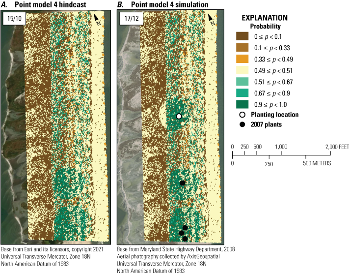
Example application of point model 4 to simulate the result of placing a planting site in a location where there have not recently been plants, Assateague Island. A is the 2008 hindcast (fig. 13, panel A, kilometer markers 6–8), and B is the simulation. Inset boxes at the upper left of each panel display the percentage of habitat probabilities greater than (>) 0.66 and > 0.9. See figures 2 and 12 for the location and aerial photographs of this region.
Transect Model Cross-Validation and Sensitivity
Eighteen BNs were constructed using transect metrics. In this section we focus on six of these BNs listed in table 4. The full set is presented in appendix 1, section 1.2. Overall, the simple and TAN BNs produced similar, and in some cases identical, performance metrics and outperformed the structured BNs (app. 1.2). Scoring metrics for the structured BNs were noticeably lower than the other network structures, and this difference was most pronounced for Kappa scores that were consistently in the moderately (0.4–0.7) or poorly (<0.4) performing range (Fielding and Bell, 1997). Like the point models, the simple versions of the transect model BNs were chosen for further exploration because of their relative simplicity and good performance scores compared to the other BN structures (app. 1.2).
Based on the results of the initial performance evaluation, we elected to use models T3 and T5 for more in-depth performance evaluation with the intent to use them for hindcasting. In addition, we included four more variations of T3 to evaluate the impact of different variables on model results. With these BNs, we conducted a performance evaluation using k-fold cross validation with five folds, and we developed five variations of the simple BN to evaluate the impact of different variables on hindcasts. Table 15 displays the results of this analysis. Calibration test error rates ranged from 3.4 to 10.4 percent, and validation scores ranged from 15.6 to 20.5 percent. The lowest error rates for both calibration and validation error rates occurred for T3. Scores for T5, which included the seed-bank variable “number of plants within 30 m,” scored comparably to T3 with error rates 0.4 and 1.7 percent higher. As with error rates, the best Kappa scores occurred for T3 (0.88 and 0.47 for calibration and validation tests, respectively). When compared to T3, its variations’ (T3b–T3e) results indicated that scores declined as fewer variables were included in the BN but indicated reasonable performance. The poorest performing BN was T3e, which was informed by morphological variables and did not include a seed-bank variable. The largest increase in error rates with respect to T3 occurred when the seed-bank proxy variables were not included in the BN (BN T3e). Based on error rates, quadratic loss, and spherical payoff, T3e performance was relatively good. On the other hand, it produced the lowest Kappa scores by a large margin (table 15).
Table 15.
Performance metrics for fivefold cross-validation using Bayesian networks used as models of seabeach amaranth habitat on Assateague Island: T3, T5, and several variations of T3.[BN, Bayesian network; no., number; T, transect; Cal., calibration; Val., validation]
T3 includes variables: shoreline change rate, distance to inlet, human modification, barrier width, mean elevation, foredune crest height, beach width and beach height, and distance to 2007 plants.
T5 includes variables: shoreline change rate, distance to inlet, human modification, barrier width, mean elevation, foredune crest height, beach width and beach height, and number of plants within 30 m from previous year.
T3b includes variables: shoreline change rate, human modification, barrier width, mean elevation, foredune crest height, beach width and beach height, and distance to 2007 plants.
T3c includes variables: shoreline change rate, barrier width, mean elevation, foredune crest height, beach width, beach height, and distance to 2007 plants.
Figure 16 shows the percentage of variance reduction for the six BNs that were examined in the performance analysis to determine the impact of each variable included (in other words, sensitivity analysis). For BNs T3 and T5, anthropogenic modification followed by mean elevation and plant proximity variables had the largest influence on hindcasts. When the distance to inlet variable was removed, the relative influence of anthropogenic modification decreased, and that of the plant proximity variable increased (fig. 16C). When anthropogenic modification was not included in the BN, the plant proximity variable had the largest influence, followed by mean elevation and barrier width (fig. 16D and E). In the last case, where the BN consisted of morphological variables only, barrier width had the largest influence on plant presence hindcasts (fig. 16F).
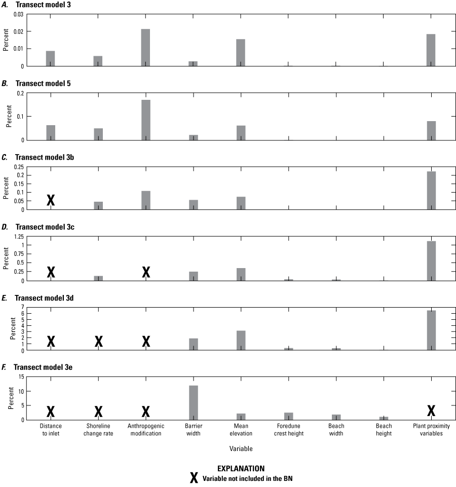
Graphs showing the percentage of variance reduction for each variable included in six different Bayesian networks (BNs) used as models of seabeach amaranth habitat on Assateague Island. A, T3, B, T5, C, T3b, D, T3c, E, T3d, and F, T3e. T, transect model.
Transect Bayesian Network Hindcasts
We used the five variations of the T3 BN and the T5 BN to hindcast the probability of plant presence for Assateague Island in 2008 (table 15, see footnote for list of variables included with each BN). This allowed us to compare BNs using different variables to determine which were required for accurate hindcasts. Like the earlier evaluation of point model performance, we also compared the percentage of habitat hindcast for KM zones where SBA were abundant (KMs 24 and 25) and not observed during the 20-year period (KM 12) to further evaluate hindcast capability. Table 16 provides a list of percentages of habitat hindcast for each zone using the six different BNs. Each BN hindcast indicated that no habitat was present for KM 12. In contrast, the BN hindcasts for KMs 24–25 indicated that between 39 and 56 percent of transects showed the probability of habitat was likely (P>0.66). In each case, all habitat probabilities were greater than 0.9 (very likely). Each of the BNs that included seed-bank variables indicated habitat presence on 54–56 percent of the transects in this region. The lowest habitat estimate was produced by T3e, which consisted of morphological variables only, did not include a seed-bank variable, and indicated that 39 percent of the region was habitat. This comparison indicates the importance of seed-bank variables for providing accurate predictions.
Table 16.
Percent habitat hindcast calculated using the transect model for two sections of Assateague Island: kilometer marker (KM) 12 (State park), where seabeach amaranth has not been observed, and KMs 24–25, where plants have been abundant.[See appendix 1, section 1.2, for the full range of hindcast results with all Bayesian networks (BNs) investigated. Numbers are percentages where P(Habitat Suitable) > 0.66/P(Habitat Suitable) > 0.9. See appendix 1, section 1.2, for full range of results. P, probability; >, greater than; KM, kilometer marker; T, transect model]
Figure 17 shows maps of the 2008 hindcasts for each of the BNs in table 16 except T5. The maps show the hindcast results for a decreasing number of variables (left to right) until only morphological metrics are included. The results show that even after the removal of distance to inlet (T3b) and anthropogenic modification variables (T3c), which provide spatial references, the hindcasts are relatively accurate at capturing habitat hotspots. Only after the distance to the previous year’s plant variables are not included do hindcast habitat probabilities appear lower in regions where SBA density is typically high (fig. 17, T3e). Comparisons of the percentages of habitat indicate that the percentage of habitat hindcast is relatively consistent for the first four BNs (T3–T3d) with a large decrease for T3e, which did not include the plant proximity variable. Despite this, BN T3e shows that some suitable habitat areas can be hindcast using morphological variables only. Here these coincide with KMs 9 and 10 and KMs 22–30, which were regions where SBA was abundant during the observation period. Table 17 displays the mean, standard deviation, maxima, and minima of variables occurring for transects where hindcasts with T3 and T3e, independently, indicated habitat (P>0.66). The mean, maxima, and minima for T3e are close to T3 but correspond more closely to observations for all the transects where SBA was observed in 2008, indicating the importance of morphological characteristics and how sustaining a seed bank influences the success of SBA.
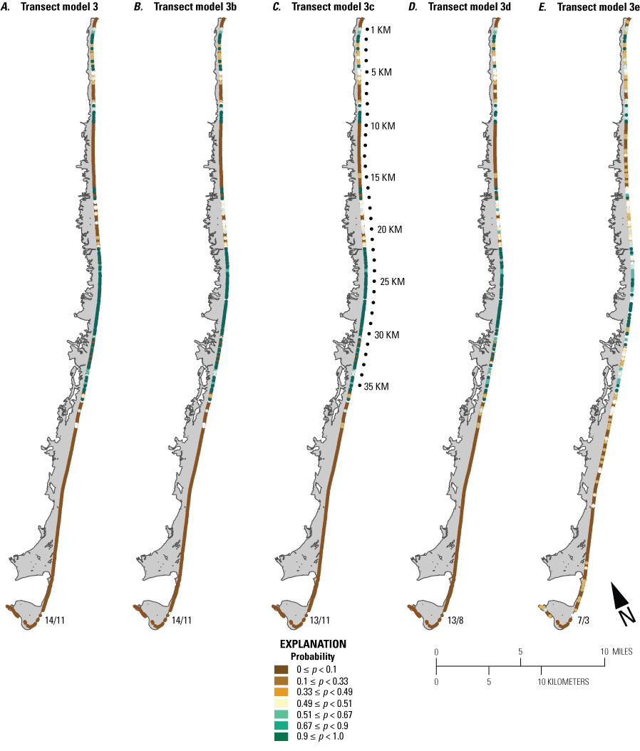
Maps of Assateague Island showing the probability of seabeach amaranth habitat using five transect (T) Bayesian networks (BNs) with different numbers of input variables. A, T3, B, T3b, C, T3c, D, T3d, and E, T3e. See the footnote of table 15 for the list of variables in BNs T3b–T3e. Numbers shown at the lower right of each map are the percentage of transects where habitat probabilities were greater than (>) 0.66 and >0.9. Kilometer markers (KM) are shown alongside the map of T3c.
Table 17.
Statistics for transects comparing morphological metrics for all transects where seabeach amaranth were observed (“w” from table 10) and for those transects where Bayesian network (BN) T3e, which contained only morphological variables (WL, MnZ, DHz, BW, BH), hindcast habitat on Assateague Island.[Std. Dev., standard deviation; Max., maximum value; Min.; minimum value; WL, barrier width; MnZ, mean elevation; DHz, foredune crest height; BW, beach width; BH, beach height; w, transects where seabeach amaranth was observed; T3e, transect model including morphology variables only; T3, transect model including all variables]
We also conducted hindcasts using the T3 BN trained on 2008 or 2014 data only and then combined 2008 and 2014 datasets to train the BN to evaluate whether morphological differences between the two datasets contributed to differences in the probabilities of habitat. Figure 18 presents four hindcast scenarios: (A) a BN trained on 2008 data and compared to 2008 transects where SBA was observed, (B) a BN trained on 2008 and 2014 data and compared to 2008 transects where SBA was observed, (C) a BN trained on 2008 data and compared to 2014 transects where SBA was observed, and (D) a BN trained on 2008 and 2014 data and compared to 2014 transects where SBA was observed. In A and B, BNs show near identical results, and transects where plants were observed correspond closely to transects where relatively high probabilities of habitat were hindcast. In C, relatively few of the hindcasts align with the observed plant locations, and many of the output probabilities were 0.5, indicating uncertain hindcasts. In D, the high probability outcomes correspond closely to the observed 2014 plant locations. The differences between C and D suggest that the morphology in 2014 differed from 2008 when SBA was more abundant on Assateague Island.
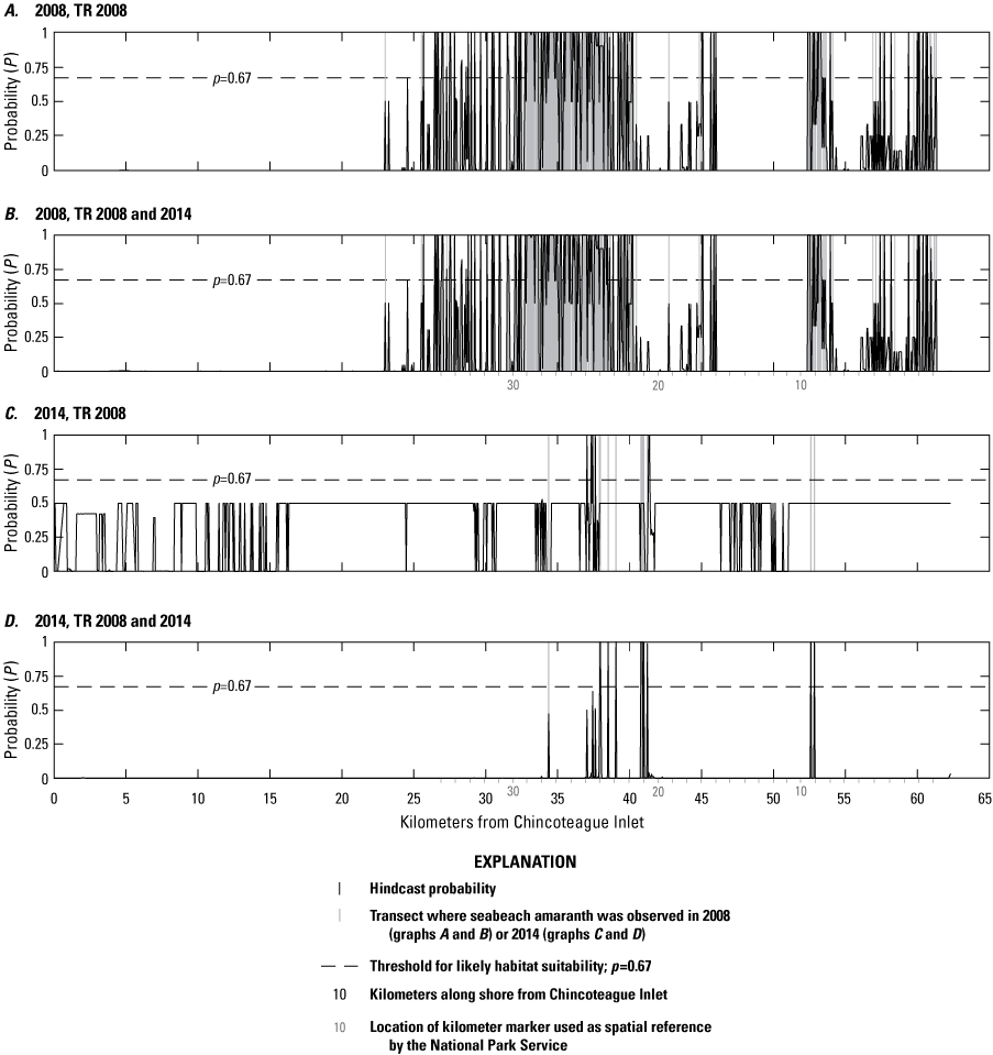
Plots showing the probability of habitat along Assateague Island for four different Bayesian networks trained (TR) with either 2008 or 2008 and 2014 data and hindcast for either 2008 or 2014. A, Hindcast for 2008 and trained with 2008 data, B, hindcast for 2008 and trained with 2008 and 2014 data, C, hindcast for 2014 and trained with 2008 data, and D, hindcast for 2014 and trained with 2008 and 2014 data. The x-axis is oriented as kilometers along shore from Chincoteague Inlet, where Chincoteague Inlet is to the left and Ocean City Inlet is to the right.
To evaluate the influence of changes in morphology and seed-bank proxies between 2008 and 2014 in more detail, we also conducted hindcasts using the T3 and T6 BNs with three different combinations of training data. For this evaluation, each BN was trained on 2008 data only, 2014 data only, and then 2008 and 2014 data together. Performance scores and the percentage of transects with habitat were calculated for Assateague Island and six of the KM zones where (a) there were no SBA observed (KMs 7 and 13), (b) no SBA was observed after 2010 (KMs 10 and 18), and (c) large numbers of SBA were observed (KMs 9 and 25) over the 20-year observation period (see table 6).
Results show that the highest performance scores occur when both 2008 and 2014 datasets are used for training. Comparison of results between BNs and years indicated that both the seed-bank proxy and morphological differences between the two time periods had an influence on the percentages of habitat. For the T3 hindcasts, when training was conducted with 2008 or 2014 data and tested with the corresponding years of data, hindcasts were relatively consistent with observations for the respective years and showed a slight tendency for underprediction for 2008 hindcasts (table 18). When testing was conducted with the opposite years, where training was conducted with 2008 and testing on 2014 and vice versa, there was a larger discrepancy in the hindcasts when compared to observations. When T3 was trained using both datasets, there was close agreement between observations and hindcasts that were nearly identical to when the BNs were trained and tested with 2008 and 2014 separately. With the T6 hindcasts, 2008 hindcasts were relatively consistent with observations for cases in which 2008 was included in the training data. In contrast, 2014 hindcasts underpredicted the amount of habitat in cases in which 2014 was included in the dataset, but overpredicted hindcasts when the BN was trained with 2008 data. In this case, 2014 hindcasts indicated that there was 9 percent more suitable habitat than was observed. Hindcasts for the KMs 13, 18, and 25 indicated habitat percentages consistent with the long-term SBA observations. Those for KMs 7 and 10 differed in that habitat was hindcast for these regions where none was observed in 2014; however, KM 10 was a site where SBA occurred frequently over the 20-year period. In addition, KM 9 hindcasts differed in that no habitat was hindcast for this zone, yet it tended to be a region where SBA was observed.
Table 18.
Error rates, spherical payoff scores, and percent of transects classified as habitat for Assateague Island and six kilometer marker zones for two Bayesian networks trained and tested with combinations of 2008 and 2014 datasets.[Habitat percentages indicate percent of habitat where P(Habitat) > 0.66 / P(Habitat) > 0.9. >, greater than; BN, Bayesian network; %, percent; Hab., habitat; KM, kilometer marker; T, transect; -, no data]
Comparison of the T3 and T6 hindcasts demonstrated differing outcomes. First, for KM 9, the percentage of habitat predicted using T6 trained with 2008 data is lower than what was observed by 30 percent (table 18, second to last row), the largest difference for any region. This could indicate the influence of seed bank on KM 9 since the same comparison for KM 10 produces a smaller difference. For the cases where T6 was trained on 2008 and tested on 2014 data, results show that there were some morphological conditions supporting habitat in 2014 that had not been habitat before (table 18, gray shading). When 2014 was added to the training, the percentage went to zero, indicating that some of the morphology in 2014 may have been habitat; the largest differences for this case were from 2014 observations for KM 7 and KM 25. For KM 7, no habitat was observed in this zone in 2008 nor 2014 and generally throughout the 20-year observation period, yet the 2014 habitat predictions computed with T6 trained with 2008 data show the presence of habitat. Similarly, the predictions made with T6 indicated that the percentage of habitat for 2014 was more than three times higher than observed when the BN was trained with 2008 data only. This suggests that by 2014, there were morphological conditions in KMs 7 and 25 comparable to 2008 habitat. Conversely, when 2014 data are added to the training for T6, the percentage of habitat for KMs 7 and 25 goes to zero. In comparison to the predictions made with T3, which included a seed-bank variable, those made with BN T6 predicted no habitat for KM 25. The results from this evaluation provide additional evidence that morphological changes and seed bank presence may have contributed to population trends, but it is not possible to isolate the impact of these changes to SBA habitat by use of the models presented here.
Discussion
Evaluation of SBA point data and barrier island transect data results indicate that there are distinct morphological conditions in which SBA occurred on Assateague Island. Elevations and distances to the ocean shoreline sampled from 2008, 2010, and 2014 for SBA plants differed from those sampled from randomly selected points on Assateague Island. Evaluation of these datasets showed SBA tended to occupy locations where (a) elevation ranged from 0.3 to 4.9 m MHW; (b) distance from the ocean shoreline was <250 m (the mean distance was 120 m); and (c) where data were available, vegetation was sparse to unvegetated. Of the three plant and random point location datasets, data from 2010 produced the fewest statistically significant differences between variables. This is likely due to the incomplete 2010 lidar dataset, in which measurements did not include the landward portions of Assateague Island.
Barrier-island transect metrics, which were examined for the 2008 and 2014 datasets, differed for those where SBA was observed versus where they were not. SBA transects had lower mean elevations and lower foredune crests compared to those where the plants were not present. In addition, the results indicate that variables serving to represent the seed bank are important components of SBA habitat. Together, results from the point and transect data support the long-held observation that the plants are prone to occur in regions subject to disturbance (for example, overwash, Weakley and others, 1996; Sellars and Jolls, 2007). Typically, these are lower-elevation regions with lower dune systems that are more susceptible to overwash during high-water events associated with storms.
The regions of Assateague Island with the most persistent presence of SBA were KMs 10, 24, and 25. Interestingly, these regions are on the upper (KM 9) and lower (KMs 24, 25) end of the elevation range for transects where plants were observed (table 10). With lower elevations, KMs 24–25 may be exposed to overwash routinely. In contrast, KM 10, which is higher than other locations where plants occur, is lower (<2 m versus >3 m) than surrounding regions to the north and south, where elevations are affected by berm and dune construction, respectively (fig. 19). In addition, surf-zone placement of sand offshore of the northern section of the barrier (see fig. 3) may provide a sediment source and maintain higher-elevation beaches and supply sand to the dune systems over time.
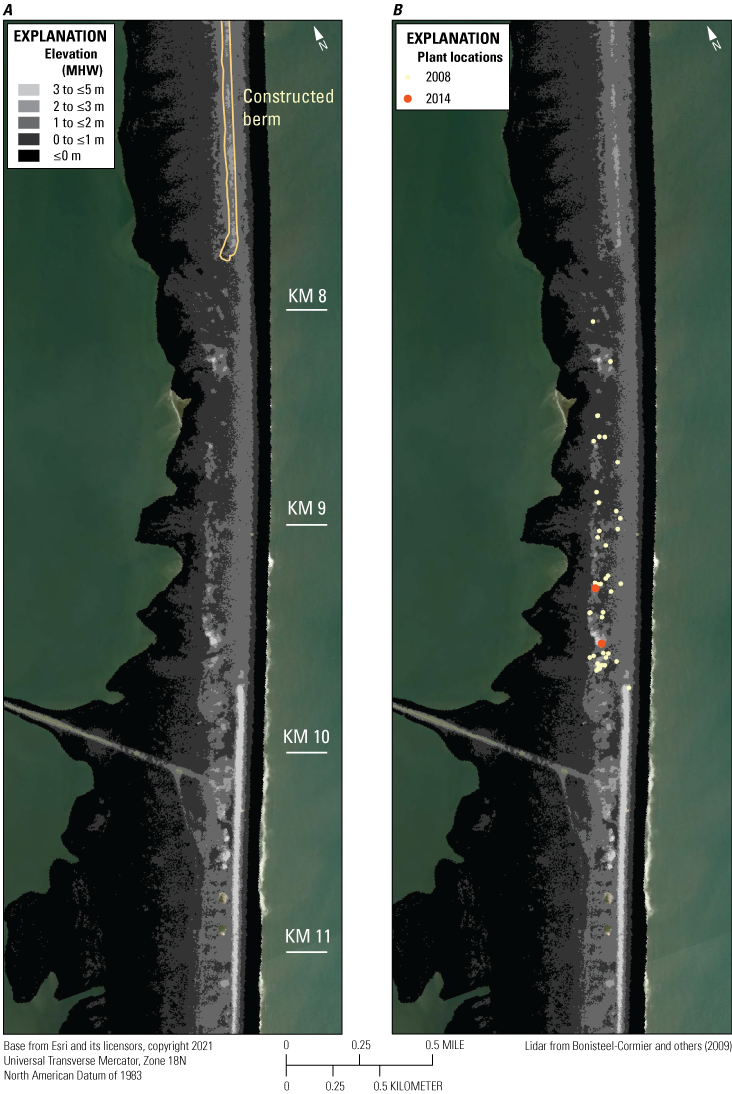
Light detection and ranging (lidar) elevation maps of northern Assateague Island between kilometer markers (KMs) 7 and 11. A, Map shows the footprint of a berm constructed in 1999 to reduce the possibility of overwash. B, Map shows the 2008 and 2014 observed seabeach amaranth locations. MHW, mean high water; m, meter; <, less than.
The development of several BNs using metrics from either point data or transect data allowed us to evaluate the two different data sampling approaches. In general, model performance for both point BNs and the transect BNs were comparable (table 13 for the former, and table 15 for the latter). The largest differences in performance were noted in the comparison of Kappa scores for validation tests where the point location BNs were in the good range (~0.7 for PM4) and the transect BN Kappa scores were in the poor to moderate range (0.25–0.47 for T3). This disparity results from the uneven numbers of transects with and without SBA in the transect datasets, which is a shortcoming of using the Kappa metric (Fielding and Bell, 1997).
For both model types, the highest performing BNs included the variables that serve as seed-bank proxies. In the absence of the seed-bank proxy variables, the models did not perform as well and produced lower certainty hindcasts. In particular, seed-bank proxy variables were important to include with the point BNs to effectively hindcast SBA presence and distinguish between high and low probability habitat (tables 14 and 15). Results showed that the barrier-island transect BN was more effective at hindcasting habitat using morphological metrics without the seed-bank proxy variables (tables 14 and 16). For the point BNs, vegetation type did not have a large impact on performance but was useful in producing more accurate hindcasts when seed-bank variables (number of plants within 30 m during the prior year and distance to nearest plant from the prior year) were not included (figs. 13–14, panels C versus D and G versus H).
When the seed-bank proxies (minimum distance to a plant from the previous year or number of plants within 30 m) were not included, habitat was hindcast in regions of ASIS where plants were absent (table 14 compared to table 16). The assumption in using the seed-bank proxy is that the previous years’ plants would be the most likely seed source for a given season. A potential shortcoming of this assumption is that SBA seeds are thought to persist for long periods of time. As a result, our choice of variables likely underestimates the presence of SBA seeds in the environment and temporal span of their influence on plant habitat.
Our analysis relied mainly on variables that could be sampled from datasets that were obtained in the years when SBA plants were observed. The metrics we sampled and analyzed were defined a posteriori, counter to recommended practices for habitat modeling (Guisan and Zimmermann, 2000; Austin, 2002; Guisan and Thuiller, 2005). This study shows that there is utility in using existing remote-sensing data to construct and evaluate habitat suitability models and analyses in absence of the ability to define optimal habitat metrics a priori. There are several examples of such studies using publicly available remote-sensing datasets to evaluate habitat for piping plover (Charadrius melodus; Gieder and others, 2014; Zeigler and others, 2017, 2019a) as well as SBA (Sellars and Jolls, 2007).
The variables included in the transect BNs provided broad measures of barrier island morphology, including beach width, island cross-section elevation and foredune height. While the transect variables were sampled at a relatively coarse resolution compared to the point data, transect BN results provided clear differences in regions of high and low habitat density (fig. 17). Part of the motivation for using the transect methods was to examine the efficacy of coarse-resolution barrier-island transect metrics (spaced at 50 m) compared to the finer-resolution (5 x 5 m) metrics used for the point model BNs. Many of the metrics used for the transect methods have been sampled from the Atlantic and Gulf coast of the United States by the USGS (Doran and others, 2017; Sturdivant and others, 2019), so the model developed here could be used to identify or examine other sites where SBA may persist.
Role of Seed Bank Versus Morphological Changes in Population Decline
Our data analysis and models of SBA habitat characteristics suggest that seed bank is an important factor contributing to habitat suitability. Both statistical comparison of point data/transect data and the evaluation of Bayesian networks using the two different data sampling schemes show that distance and number of plants near a site in the previous year are important factors contributing to higher probability habitat. Even so, from the analysis of transect metrics, we cannot rule out that changes in morphology also contributed to SBA decline. From our comparison of 2008 to 2014 transects, we found that where plants were present, transect metrics were similar from 2008 to 2014 (table 11). Alternatively, when we compared the morphology of the specific transects where plants were observed in 2008 to those in 2014, we found that locations that did not contain plants in 2014 were statistically different than they had been in 2008.
Comparison of model results from BNs T3 and T6 and the different training and testing dataset combinations provided additional evidence that both seed bank and morphology have large influences on habitat presence such that it is difficult to isolate the influence of one over the other in our analysis (table 18). When tested with the transect BNs, 2014 hindcasts that included the seed-bank variable (T3) and were trained using 2008 data did not produce hindcasts that corresponded to 2014 observations (fig. 18C; table 18). Only when 2014 data were included in the BN training data was a higher correspondence between 2014 hindcasts and observations observed (fig. 18D; table 18). It is surprising that with the addition of just 12 transects with SBA in 2014 (versus 196 in 2008), hindcast performance for 2014 increased markedly. Far less habitat was hindcast for 2014 using the training of both datasets, but that which was hindcast accurately could be done so for both 2008 and 2014 and produced results that corresponded closely to observed 2008 and 2014 sites. In addition, hindcasts conducted with a BN that did not include a seed-bank proxy variable (T6) provided additional evidence that we could not rule out the influence of morphological changes in SBA population decline. For the case in which the training was conducted with 2008 data and the hindcast was applied for 2014, the relative abundance of hindcast 2014 habitat indicates that morphological conditions in 2014 may have changed sufficiently to generate higher probabilities of habitat. However, it is not possible to isolate the influence of morphology from that of the seed bank as the prevalence of 2008 habitat was likely influenced by the abundance of SBA in prior years. Analyses of additional data could help to determine if changes in morphology led to a decline in the SBA population. As noted previously, detailed studies of morphological changes in the KMs 6–8 region where berm construction occurred may be a site where this could be investigated in greater depth.
Population Decline and Implications for SBA Management
Both the population trends and model results suggest that a sustained effort to plant SBA was effective in establishing a viable population on Assateague Island. While the single-year population never exceeded the ~5,000 plantings between 2000 and 2002, the SBA population exceeded at least 500 plants for 9 years after the last planting effort in 2002. In addition, from 2003 to 2009, SBA was observed in at least 25 of the 36 KM zones along the Maryland portion of ASIS (table 6). By 2010, the number of plants decreased to 203, from 1,260 in 2009, and the number of occupied KM zones decreased to 16. We have noted that the population decline occurred over a period of 3 years when drought conditions persisted during the typical germination periods of the plants and speculate that drought may have contributed to population decline. Strong storms also occurred during this period (Nor’Ida, November 2009; Hurricane Irene, August 2011; Superstorm Sandy, October 2012) and led to substantial erosion and changes to island morphology. This suggests that SBA seeds may have been removed from the barrier island by erosion or buried in washover deposits to a sufficient depth that they prevented germination in the following seasons. In addition, during this period, population numbers may have been low enough that grazing also reduced plant viability but, given that most of the grazing was by insects, it is unclear if this would have affected the ability of the plants to produce seeds for dispersal. Further investigation is needed to see if it is possible to observe storm impacts at sites where SBA may be present.
Our analysis suggests that it will be important to conduct planting efforts to sustain the population over the long term. In a natural state, seeds from adjacent barrier islands (Fenwick Island to the north and Wallops Island to the south) could be sources for Assateague Island, but it is unknown if SBA is present at these sites, both of which are highly developed and have undergone significant shoreline and (or) erosion management efforts. Ideally, to sustain the Assateague Island population, planting would occur after seasons of substantial population decreases. More study is needed to determine if there is a critical population size that is required to sustain a long-term population. From our examination of the 20-year record at Assateague Island, planting cultivated SBA plants may be optimal following large population declines, such as in 2008 when the population decreased by half or after 2010 when the population declined by 84 percent (1,260 to 203 plants).
A deeper understanding of seed-bank dynamics and dispersal pathways could help improve understanding of SBA population trends. During the initial few years, plants dispersed up to 6–7 km from the previous year’s planting sites. In 2001 and 2002, the regions with the largest numbers of plants were regions planted the previous year. By 2003, plants were widely dispersed, suggesting robust natural dispersal. From the four regions planted in 2000, there were 22 regions where wild plants were observed in 2001, increasing to 27 regions in 2002 and 33 regions in 2003, despite a population decrease of nearly 400. Such spread suggests conditions were suitable for natural dispersion during these years. Following the substantial decline in 2010, the SBA population ranged from 203 to 251 plants for three seasons before dropping to 8 individuals in 2013. By 2015, the population reached 122 plants, almost all of which were located at KMs 9 and 25; two regions where plants were observed most often. Despite plants tending to be most common in these regions, even when population was small, it is unknown if the seeds that sustained this population were from the previous year’s plants or had germinated from older seed stock buried on the barrier island.
Regions of Limited SBA Presence and Disturbances
Examination of the SBA population distribution clearly shows that plants are generally absent from two areas on the Maryland portion of Assateague Island (table 6): KMs 5–8 (berm region) and the Assateague State Park region through the beginning of the OSV zone (KMs 11–16, see figs. 2 and 3). Both are areas where the barrier morphology is influenced by human activity. Within the State-park region, barrier-island transect BN hindcasts for KM 13 showed no habitat for any of the hindcast cases (table 16). This suggests that areas where recreational activity is more frequent may not be suitable for plants due to a combination of factors: morphology, lack of seed sources, and recreational use impacts. In addition, the activities undertaken to maintain the infrastructure in KM 13 (construction of dunes and placement of sand fencing) contribute to the maintenance of barrier-island morphology (in other words, higher beaches and dunes) that is not associated with SBA.
Hindcasts for 2014 using the T6 BN trained with 2008 data indicated that the morphology of the KM 7 region was suitable for habitat. This is notable since this region occurred where passageways for overwash were bulldozed to allow periodic overwash to improve piping plover habitat (Schupp and others, 2013). Furthermore, it was noted that overwash occurred in this region twice in the fall of 2009. Since then, there have been other events when overwash occurred at these locations (Hurricane Irene, 2011; Superstorm Sandy, 2012), but we did not have the opportunity to do an in-depth evaluation of the morphological changes that occurred before and after such events and if they resulted in changes to habitat probabilities. As noted earlier, SBA is a plant species that relies on disturbance in the form of high-water events that cause overwash to occur in beach and barrier-island settings, which often results in a flattening of the dune system and consequent deposition of washover sand flats that extend into low-lying interior portions of barrier islands (Morton and Sallenger, 2003). Future studies of long-term morphological changes and frequency of overwash and its contribution to increasing SBA habitat on the north section of ASIS in the regions including and surrounding KM 7 can provide more understanding of the importance of overwash to this species.
Future Data Needs for Evaluating SBA Habitat
If there is an opportunity to collect additional data on SBA habitat, there are a few parameters that should be included: (a) soil moisture, (b) direct observations of high-water impacts to plants, (c) on-the-ground photographs of SBA sites, and (d) plant fate. Soil-moisture measurements would provide a direct means of evaluating the impact of drought on SBA seed germination success. Monitoring of high-water events would provide information on the timing and spatial distribution of plant disturbance and habitat creation and assist in evaluating the effect of high-water events on plant fate. While washover deposits appear to be important for SBA habitat, the plants have low tolerance to direct saltwater exposure (Weakley and others, 1996). Consequently, the timing of overwash events may be important, with those occurring during seed germination and prior to seed dispersal in the fall being detrimental, since SBA plants are thought not to be tolerant of direct exposure to salt water (Weakley and others, 1996). Additional details regarding the geomorphic settings where plants are observed may help in better understanding the specific beach and barrier-island subenvironments where these plants are most successful. Photographs of the plant locations and surroundings could be used to identify geomorphic environments (for example, washover flats versus foredune regions), sediment grain size, and proximity to wrack, which may serve as a trap for seeds and influence substrate moisture. Lastly, observations of plant fate are important, particularly if SBA survives long enough to produce seeds that are dispersed.
Summary
Amaranthus pumilus (seabeach amaranth; SBA), once ubiquitous on the mid-Atlantic coast of the United States, has rarely been found at Assateague Island National Seashore over the last century. This plant species tends to occur in natural beach and barrier island settings where disturbance in the form of occasional flooding and erosion due to storms creates suitable habitat. At Assateague Island, an effort to re-establish seabeach amaranth over three seasons established a population on the barrier island that persisted for nearly 20 years. For more than a decade, the plant population exceeded 500 individuals and declined over the remaining period such that no plants have been observed in the last three years (2018–21). Results from analyzing point data obtained at observed plant locations and randomly selected points indicate that SBA occurs at settings that are distinct from randomly selected locations. In addition, barrier island metrics where SBA occurs exhibited differences from both randomly selected locations and all locations for some metrics (mean elevation, foredune crest height, beach height). Distinctions were less clear for data from 2014 when the SBA occurrence was substantially lower than in 2008. In general, SBA habitat tended to occur on regions of the island that were lower in mean elevation, beach height, and exhibited lower foredune crest elevations.
The two modeling approaches using Bayesian networks (BNs) we developed performed well. Both BN approaches produced comparable performance scores, with the point model exhibiting slightly higher scores than the transect model. Despite this, the transect model produced hindcasts that consistently distinguished SBA habitat from nonhabitat areas irrespective of the variables included in the BN. Analysis of point data and barrier island transect data in addition to the BN model results indicate that variables serving as proxies for seed bank are important to include in models to accurately distinguish SBA habitat from nonhabitat regions. The two variables that we considered, distance to the nearest plant from the previous year and number of plants within 30 meters, produced well-performing BNs, with the former resulting in slightly better model performance. We were unable to determine conclusively that morphological changes in island characteristics contributed directly to SBA population decline. We speculate that population decline occurred due to a combination of factors, wherein the largest declines co-occurred with successive years of drought and significant storm impacts to Assateague Island. It is possible that the combination and timing of these factors contributed to a decrease in viable seeds on the barrier island to a point where the population was unable to sustain itself. Our analysis of SBA habitat data and model results suggest that it is important to allow overwash to create suitable substrate for SBA and to maintain planting efforts to sustain the population.
References Cited
Austin, M.P., 2002, Spatial prediction of species distribution—An interface between ecological theory and statistical modelling: Ecological Modelling, v. 157, nos. 2–3, p. 101–118, accessed April 16, 2020, at https://doi.org/10.1016/S0304-3800(02)00205-3.
Bayes, T., 1763, An essay towards solving a problem in the doctrine of chances: Philosophical Transactions of the Royal Society of London, v. 53, p. 370–418. [Also available at https://doi.org/10.1098/rstl.1763.0053.]
Beguería, S., Latorre, B., Reig, F., and Vincente-Serrano, S.M., 2022, Standardized precipitation evapotranspiration index (SPEI): Global Drought Monitor data, accessed June 10, 2022, at https://spei.csic.es/map/maps.html.
Bonisteel, J.M., Nayegandhi, A., Brock, J., Wright, C.W., Stevens, S., Yates, X., and Klipp, E.S., 2009, EAARL coastal topography–Assateague Island National Seashore, 2008—Bare earth: U.S. Geological Survey Data Series 447, [1 DVD], accessed October 2019 at https://doi.org/10.3133/ds447.
Bonisteel-Cormier, J.M., Nayegandhi, A., Wright, C.W., Brock, J.C., Nagle, D.B., Vivekanandan, S., Klipp, E.S., Fredericks, X., and Stevens, S., 2011, EAARL coastal topography—Assateague Island National Seashore, Maryland and Virginia, 2010: U.S. Geological Survey Data Series 628, [1 DVD], accessed June 2021 at https://doi.org/10.3133/ds628.
Chase, J.B., Huslander, B., Strum, M., Lea, C., Gutierrez, B.T., and Sterne, T.K., 2023, Assateague Island seabeach amaranth survey data—2001 to 2018: U.S. Geological Survey data release, https://doi.org/10.5066/P9IZMQ1B.
Cowell, R., 1998, Introduction to inference for Bayesian networks, in Jordan, M.I., ed., Learning in graphical models [NATO ASI Series]: Dordrecht, Springer, v. 89, p. 9–26. [Also available at https://doi.org/10.1007/978-94-011-5014-9_1.]
Dean, R.G., and Perlin, M., 1977, A coastal engineering study of Ocean City Inlet, in Proceedings of Coastal Sediments ’77, fifth Symposium of the Waterway, Port, Coastal, and Ocean Division of ASCE, Charleston, South Carolina, November 2–4, 1977: Reston, Virginia, American Society of Civil Engineers, p. 520–540.
Dempster, A.P., Laird, N.M., and Rubin, D.B., 1977, Maximum likelihood from incomplete data via the EM algorithm: Journal of the Royal Statistical Society—Series B (Methodological), v. 39, no. 1, p. 1–22, accessed May 18, 2015, at https://doi.org/10.1111/j.2517-6161.1977.tb01600.x.
Doran, K.S., Long, J.W., Birchler, J.J., Brenner, O.T., Hardy, M.W., Morgan, K.L.M., Stockdon, H.F., and Torres, M.L., 2017, Lidar-derived beach morphology (dune crest, dune toe, and shoreline) for U.S. sandy coastlines (ver. 4.0, October 2020): U.S. Geological Survey data release, accessed May 2019 at https://doi.org/10.5066/F7GF0S0Z.
Fielding, A.H., and Bell, J.F., 1997, A review of methods for the assessment of prediction errors in conservation presence/absence models: Environmental Conservation, v. 24, no. 1, p. 38–49, accessed May 11, 2021, at https://doi.org/10.1017/S0376892997000088.
Fienen, M.N., Masterson, J.P., Plant, N.G., Gutierrez, B.T., and Thieler, E.R., 2013, Bridging groundwater models and decision support with a Bayesian network: Water Resources Research, v. 49, no. 10, p. 6459–6473. [Also available at https://doi.org/10.1002/wrcr.20496.]
Fienen, M.N., and Plant, N.G., 2015, A cross-validation package driving Netica with python: Environmental Modelling & Software, v. 63, p. 14–23, accessed April 4, 2018, at https://doi.org/10.1016/j.envsoft.2014.09.007.
Friedman, N., Geiger, D., and Goldszmidt, M., 1997, Bayesian network classifiers: Machine Learning, v. 29, no. 2, p. 131–163, accessed August 14, 2012, at https://doi.org/10.1023/A:1007465528199.
Gieder, K.D., Karpanty, S.M., Fraser, J.D., Catlin, D.H., Gutierrez, B.T., Plant, N.G., Turecek, A.M., and Thieler, E.R., 2014, A Bayesian network approach to predicting nest presence of the federally-threatened piping plover (Charadrius melodus) using barrier island features: Ecological Modelling, v. 276, p. 38–50. [Also available at https://doi.org/10.1016/j.ecolmodel.2014.01.005.]
Guisan, A., and Thuiller, W., 2005, Predicting species distribution—Offering more than simple habitat models: Ecology Letters, v. 8, no. 9, p. 993–1009, accessed April 15, 2020, at https://doi.org/10.1111/j.1461-0248.2005.00792.x.
Guisan, A., and Zimmermann, N.E., 2000, Predictive habitat distribution models in ecology: Ecological Modelling, v. 135, nos. 2–3, p. 147–186, accessed May 23, 2019, at https://doi.org/10.1016/S0304-3800(00)00354-9.
Gutierrez, B.T., Heslin, J.L., Henderson, R.E., Sterne, T.K., and Sturdivant, E.J., 2023, Seabeach amaranth presence-absence and barrier island geomorphology metrics as relates to shorebird habitat for Assateague Island National Seashore—2008, 2010, and 2014: U.S. Geological Survey data release, https://doi.org/10.5066/P9GKXN3H.
Gutierrez, B.T., Plant, N.G., and Thieler, E.R., 2011, A Bayesian network to predict coastal vulnerability to sea level rise: Journal of Geophysical Research [Earth Surface], v. 116, no. F2, article number F02009, 15 p. [Also available at https://doi.org/10.1029/2010JF001891.]
Gutierrez, B.T., Plant, N.G., Thieler, E.R., and Turecek, A., 2015, Using a Bayesian network to predict barrier island geomorphologic characteristics: Journal of Geophysical Research [Earth Surface], v. 120, no. 12, p. 2452–2475. [Also available at https://doi.org/10.1002/2015JF003671.]
Guttman, N.B., 1999, Accepting the Standardized precipitation index—A calculation algorithm: Journal of the American Water Resources Association, v. 35, no. 2, p. 311–322, accessed May 20, 2020, at https://doi.org/10.1111/j.1752-1688.1999.tb03592.x.
Hapke, C.J., Himmelstoss, E.A., Kratzmann, M.G., List, J.H., and Thieler, E.R., 2011, National assessment of shoreline change—Historical shoreline change along the New England and Mid-Atlantic coasts: U.S. Geological Survey Open-File Report 2010–1118, 57 p. [Also available at https://doi.org/10.3133/ofr20101118.]
Heckerman, D., 1998, A tutorial on learning with Bayesian networks, in Jordan, M.I., ed., Learning in graphical models [NATO ASI Series]: Dordrecht, Springer, p. 301–354. [Also available at https://doi.org/10.1007/978-94-011-5014-9_11.]
Himmelstoss, E.A., Kratzmann, M.G., Hapke, C., Thieler, E.R., and List, J., 2010, The national assessment of shoreline change—A GIS compilation of vector shorelines and associated shoreline change data for the New England and Mid-Atlantic Coasts: U.S. Geological Survey Open-File Report 2010–1119, accessed May 2019 at https://doi.org/10.3133/ofr20101119.
Jensen, F.V., and Nielsen, T.D., 2007, Bayesian networks and decision graphs: New York, Springer, 447 p. [Also available at https://doi.org/10.1007/978-0-387-68282-2.]
Jiang, L., Cai, Z., Wang, D., and Zhang, H., 2012, Improving tree augmented naive Bayes for class probability estimation: Knowledge-Based Systems, v. 26, p. 239–245. [Also available at https://doi.org/10.1016/j.knosys.2011.08.010.]
Keyantash, J., and National Center for Atmospheric Research [NCAR] Staff, eds., 2019, The climate data guide—Standardized precipitation index (SPI): National Center for Atmospheric Research data, accessed June 9, 2022, at https://climatedataguide.ucar.edu/climate-data/standardized-precipitation-index-spi.
Krantz, D.E., Schupp, C.A., Spaur, C.C., Thomas, J.E., and Wells, D.V., 2009, Dynamic systems at the land-sea interface, chap. 12 of Dennison, W.C., Thomas, J.E., Cain, C.J., Carruthers, T.J.B., Hall, M.R., Jesien, R.V., Wazniak, C.E., and Wilson, D.E., eds., Shifting sands—Environmental and cultural change in Maryland’s coastal bays: Cambridge, Md., University of Maryland Center for Environmental Science, Integration and Application Network (IAN) Press, p. 211–248.
Lauritzen, S.L., 1995, The EM algorithm for graphical association models with missing data: Computational Statistics & Data Analysis, v. 19, no. 2, p. 191–201. [Also available at https://doi.org/10.1016/0167-9473(93)E0056-A.]
Marcot, B.G., 2012, Metrics for evaluating performance and uncertainty of Bayesian network models: Ecological Modelling, v. 230, p. 50–62, accessed March 23, 2012, at https://doi.org/10.1016/j.ecolmodel.2012.01.013.
Marcot, B.G., Woo, I., Thorne, K.M., Freeman, C.M., and Guntenspergen, G.R., 2020, Habitat of the endangered salt marsh harvest mouse (Reithrodontomys raviventris) in San Francisco Bay: Ecology and Evolution, v. 10, no. 2, p. 662–677, accessed September 3, 2020, at https://doi.org/10.1002/ece3.5860.
Maryland Geological Survey, 2006, High resolution shoreline map data for Tidewater Maryland: Maryland Geological Survey data, accessed July 2012 at http://www.mgs.md.gov/coastal_geology/hi%20res%20shoreline.html.
Massey, F.J., 1951, The Kolmogorov-Smirnov test for goodness of fit: Journal of the American Statistical Association, v. 46, no. 253, p. 68–78, accessed March 13, 2023, at https://doi.org/10.2307/2280095.
Mastrandrea, M.D., Field, C.B., Stocker, T.F., Edenhofer, O., Ebi, K.L., Frame, D.J., Held, H., Kriegler, E., Mach, K.J., Matschoss, P.R., Plattner, G.-K., Yohe, G.W., and Zwiers, F.W., 2010, Guidance note for lead authors of the IPCC Fifth Assessment Report on consistent treatment of uncertainties: Geneva, Intergovernmental Panel on Climate Change (IPCC), 4 p. [Also available at https://www.ipcc.ch/site/assets/uploads/2017/08/AR5_Uncertainty_Guidance_Note.pdf.]
Morgan, M.G., and Henrion, M., 1990, Uncertainty—A guide to dealing with uncertainty in quantitative risk and policy analysis: Cambridge, United Kingdom, Cambridge University Press, 332 p. [Also available at https://doi.org/10.1017/CBO9780511840609.]
Morton, R.A., Bracone, J.E., and Cooke, B., 2007, Geomorphology and depositional sub-environments of Assateague Island MD/VA: U.S. Geological Survey Open-File Report 2007–1388, accessed May 8, 2010, at https://doi.org/10.3133/ofr20071388.
National Oceanic and Atmospheric Administration [NOAA], 2018, Vertical datum transformation: National Oceanic and Atmospheric Administration database, accessed September 4, 2018, at https://vdatum.noaa.gov/.
National Oceanic and Atmospheric Administration [NOAA], 2020, Standardized precipitation index—Drought indices and data: National Oceanic and Atmospheric Administration data, accessed August 31, 2020, at https://www.ncdc.noaa.gov/temp-and-precip/drought/nadm/indices/spi/div#select-form.
National Park Service [NPS], 2008, Assateague Island National Seashore north end piping plover habitat 2008: National Park Service dataset, accessed May 2019 at https://asis-nps.opendata.arcgis.com/datasets/asis-pipl-habitat2008/.
National Park Service [NPS], 2010, Assateague Island National Seashore north end piping plover habitat 2010: National Park Service dataset, accessed October 2021 at https://asis-nps.opendata.arcgis.com/datasets/asis-pipl-habitat-2010/.
National Park Service [NPS], 2014, Assateague Island National Seashore north end piping plover habitat collected 2014: National Park Service dataset, accessed May 2019 at https://asis-nps.opendata.arcgis.com/datasets/asis-pipl-habitat2014/.
Oertel, G.F., and Kraft, J.C., 1994, New Jersey and Delmarva barrier-islands, chap. 6 of Davis, R.A., Jr., ed., Geology of Holocene barrier island systems: Berlin, Springer, p. 207–232. [Also available at https://doi.org/10.1007/978-3-642-78360-9_6.]
Pearl, J., 1978, An economic basis for certain methods of evaluating probabilistic forecasts: International Journal of Man-Machine Studies, v. 10, no. 2, p. 175–183, accessed April 1, 2010, at https://doi.org/10.1016/S0020-7373(78)80010-8.
Runge, M.C., 2011, An introduction to adaptive management for threatened and endangered species: Journal of Fish and Wildlife Management, v. 2, no. 2, p. 220–233. [Also available at https://doi.org/10.3996/082011-JFWM-045.]
Sallenger, A.H., Jr., 2000, Storm impact scale for barrier islands: Journal of Coastal Research, v. 16, no. 3, p. 890–895. [Also available at https://www.jstor.org/stable/4300099.]
Schupp, C.A., Winn, N.T., Pearl, T.L., Kumer, J.P., Carruthers, T.J.B., and Zimmerman, C.S., 2013, Restoration of overwash processes creates piping plover (Charadrius melodus) habitat on a barrier island (Assateague Island, Maryland): Estuarine, Coastal and Shelf Science, v. 116, p. 11–20, accessed January 28, 2013, at https://doi.org/10.1016/j.ecss.2012.07.003.
Sellars, J.D., and Jolls, C.L., 2007, Habitat modeling for Amaranthus pumilus—An application of light detection and ranging (LIDAR) data: Journal of Coastal Research, v. 23, no. 5, p. 1193–1202, accessed March 21, 2019, at https://doi.org/10.2112/04-0334.1.
Stockdon, H.F., Doran, K.S., and Sallenger, A.H., Jr., 2009, Extraction of lidar-based dune-crest elevations for use in examining the vulnerability of beaches to inundation during hurricanes: Journal of Coastal Research, v. 53, no. 10053, p. 59–65, accessed October 2, 2012, at https://doi.org/10.2112/SI53-007.1.
Stockdon, H.F., Doran, K.S., Thompson, D.M., Sopkin, K.L., Plant, N.G., and Sallenger, A.H., Jr., 2012, National assessment of hurricane-induced coastal erosion hazards—Gulf of Mexico: U.S. Geological Survey Open-File Report 2012–1084, 51 p. [Also available at https://doi.org/10.3133/ofr20121084.]
Sturdivant, E.J., Zeigler, S.L., Gutierrez, B.T., and Weber, K.M., 2019, Barrier island geomorphology and shorebird habitat metrics—Sixteen sites on the U.S. Atlantic Coast, 2013–2014: U.S. Geological Survey data release, accessed May 2019 at https://doi.org/10.5066/P9V7F6UX.
Tyndall, R.W., Ramsey, S., and Lea, C., 2000, The federally threatened Amaranthus pumilus Raf. (seabeach amaranth, Amaranthaceae) rediscovered on Assateague Island after 31 years: Castanea, v. 65, no. 2, p. 165–167. [Also available at https://www.jstor.org/stable/4034115.]
U.S. Fish and Wildlife Service [USFWS], 1993, Endangered and threatened wildlife and plants; Amaranthus pumilus (seabeach amaranth) determined to be threatened: Federal Register, v. 58, no. 65, p. 18035–18042, accessed June 7, 2022, at https://archives.federalregister.gov/issue_slice/1993/4/7/18029-18042.pdf#page=7.
U.S. Fish and Wildlife Service, 2021, Seabeach amaranth (Amaranthus pumilus): U.S. Fish and Wildlife Service Environmental Conservation Online System (ECOS) data, accessed June 7, 2022, at https://ecos.fws.gov/ecp/species/8549.
Vincente-Serrano, S.M., Beguería, S., and López-Moreno, J.I., 2010, A multiscalar drought index sensitive to global warming—The standardized precipitation evapotranspiration index: Journal of Climate, v. 23, no. 7, p. 1696–1718. [Also available at https://doi.org/10.1175/2009JCLI2909.1.]
Vincente-Serrano, S.M., and National Center for Atmospheric Research Staff, eds., 2015, The climate data guide—Standardized precipitation evapotranspiration index (SPEI): National Center for Atmospheric Research web page, accessed June 10, 2022, at https://climatedataguide.ucar.edu/climate-data/standardized-precipitation-evapotranspiration-index-spei.
Weakley, A., Bucher, M., and Murdoch, N., 1996, Recovery plan for seabeach amaranth (Amaranthus pumilus): U.S. Fish and Wildlife Service report, 59 p. [Also available at https://ecos.fws.gov/docs/recovery_plan/961112b.pdf.]
Weber, K.M., List, J.H., and Morgan, K.L.M., 2005, An operational mean high water datum for determination of shoreline position from topographic lidar data: U.S. Geological Survey Open-File Report 2005–1027, accessed July 2012 at https://doi.org/10.3133/ofr20051027.
Zeigler, S.L., Gutierrez, B.T., Hecht, A., Plant, N.G., and Sturdivant, E.J., 2021, Piping plovers demonstrate regional differences in nesting habitat selection patterns along the U.S. Atlantic coast: Ecosphere, v. 12, no. 3., 21 p. [Also available at https://doi.org/10.1002/ecs2.3418.]
Zeigler, S.L., Gutierrez, B.T., Sturdivant, E.J., Catlin, D.H., Fraser, J.D., Hecht, A., Karpanty, S.M., Plant, N.G., and Thieler, E.R., 2019a, Using a Bayesian network to understand the importance of coastal storms and undeveloped landscapes for the creation and maintenance of early successional habitat: PLOS ONE, v. 14, no. 7, 30 p. [Also available at https://doi.org/10.1371/journal.pone.0209986.]
Zeigler, S.L., Sturdivant, E.J., and Gutierrez, B.T., 2019b, Evaluating barrier island characteristics and piping plover (Charadrius melodus) habitat availability along the U.S. Atlantic coast—Geospatial approaches and methodology (ver. 1.1, October 2019): U.S. Geological Survey Open File Report 2019–1071, 34 p. [Also available at https://doi.org/10.3133/ofr20191071.]
Zeigler, S.L., Thieler, E.R., Gutierrez, B.T., Plant, N.G., Hines, M., Fraser, J.D., Catlin, D.H., and Karpanty, S.M., 2017, Smartphone technologies and Bayesian networks to assess shorebird habitat selection: Wildlife Society Bulletin, v. 41, no. 4, p. 666–677. [Also available at https://doi.org/10.1002/wsb.820.]
Appendix 1. Bayesian Network Configuration, Initial Performance Testing and Scores, and Hindcast Evaluation
1.1. Bayesian Network Configuration and Initial Performance Testing
We developed 24 different Bayesian network (BN) models for the presence-absence data and 18 different BNs for the transect data. The BNs for each were configured using three different model structures (simple, structured, TAN) (tables 1.1 and 1.2). Each of the model structures represents three different assumptions. The first model structure consisted of nodes all connected to “plant presence” indicating that each variable had equal influence on seabeach amaranth (SBA) habitat (figs. 5A and 5D). The second model structure included connections between variables that were thought to have an influence on one another (figs. 5B and E). The last model structure was determined using a tree-augmented naïve Bayes (TAN) algorithm that can calculate the optimal BN structure (Friedman and others, 1997; figs. 5C and 5F). This algorithm, implemented via Netica software, uses a modified naive Bayes learning rule to evaluate the optimal BN structure for a specified dependent variable. The three model structures were used as a point of comparison where models of differing complexity and an optimized model (TAN) could be compared to determine potential outcome variability.
For each BN structure, several BNs were constructed consisting of different combinations of variables (tables 1.1 and 1.2). We used the correlation coefficients between variables to eliminate variables that were correlated from the BN (see tables 9 and 12). We then varied the number of variables in each model structure. This resulted in removing the vegetation type variable and developing networks with and without the seed-bank variables. For BNs constructed using the TAN algorithm, two versions of each network were created: one with arrows pointing from the response variable (habitat probability) to independent variables, and vice versa. We pursued this after noticing that BN performance differed depending on the direction of the links between the response variable and independent variable. Developing and evaluating BNs with differing structures and variables allowed us to develop reference comparisons for different BNs and understand the range of possible results.
Table 1.1.
Variables included in, and configurations of, the point model Bayesian networks for Assateague Island data.[no., number; DisMHW, the distance to mean high water variable; VT, vegetation type; No_30, number of plants within 30 meters from the previous year; Dnp, the distance to the nearest plant from the previous year; PM, point model; “-o” designates that edges point away from the posterior node; TAN, tree-augmented naïve Bayes algorithm; X (with shading), variable included in the Bayesian network; - (without shading), variable was not included]
Table 1.2.
Variables included in, and configurations of, the transect model Bayesian networks for Assateague Island data.[no., number; Nour, nourishment; Const., constructed features; Devel., development; Dist. to Inlet, distance to Ocean City Inlet; No_30, number of plants within 30 meters from the previous year; D_trans, distance to the nearest plant from the previous year; T, transect model; TAN, tree-augmented naïve Bayes algorithm; X (with shading), variable included in the BN; - (without shading), variable was not included]
The following figures show examples of selected BNs from tables 1.1 and 1.2. The BNs shown were selected to provide examples of the three structures and how the input variables were binned in each node. BNs with the maximum number of variables are displayed. For cases where fewer variables were included, those nodes and their connections (edges) were eliminated from the respective BNs. The structure of BNs that were developed using the TAN algorithm varies according to the influence of the variables used for the network. Only two of these structures, point model (7 variables) and transect model (10 variables), are shown in the following figures (figs. 1.1–1.9).
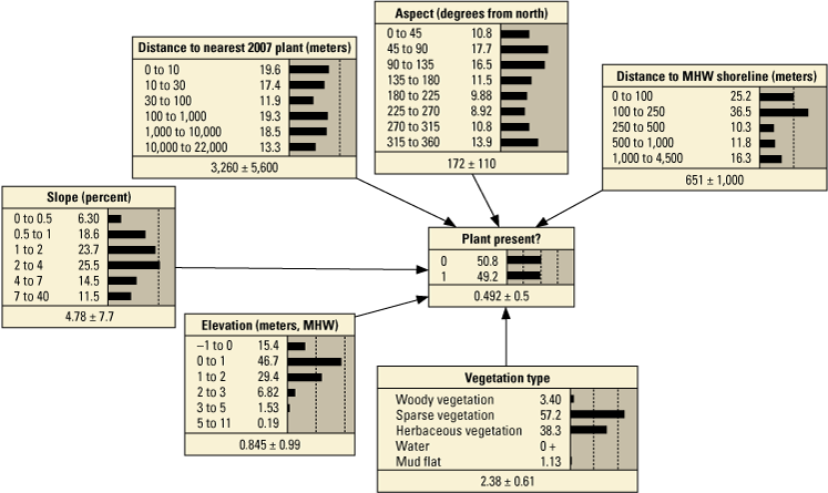
Bayesian network (BN) for point model (PM) 3: BN trained using data from 2008. Dashed vertical lines indicate 25, 50, and 75 percent. MHW, mean high water.
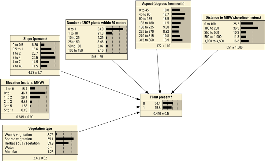
Bayesian network (BN) for point model (PM) 1: BN trained using data from 2008. Dashed vertical lines indicate 25, 50, and 75 percent. MHW, mean high water.
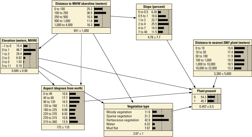
Bayesian network (BN) for point model (PM) 9: BN trained using data from 2008. Dashed vertical lines indicate 25, 50, and 75 percent. MHW, mean high water.
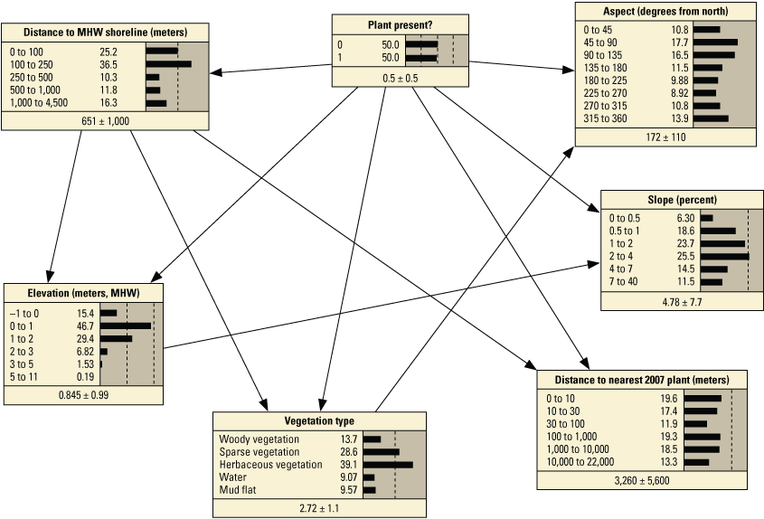
Bayesian network (BN) for point model (PM) 17: BN trained using data from 2008. Dashed vertical lines indicate 25, 50, and 75 percent. MHW, mean high water.
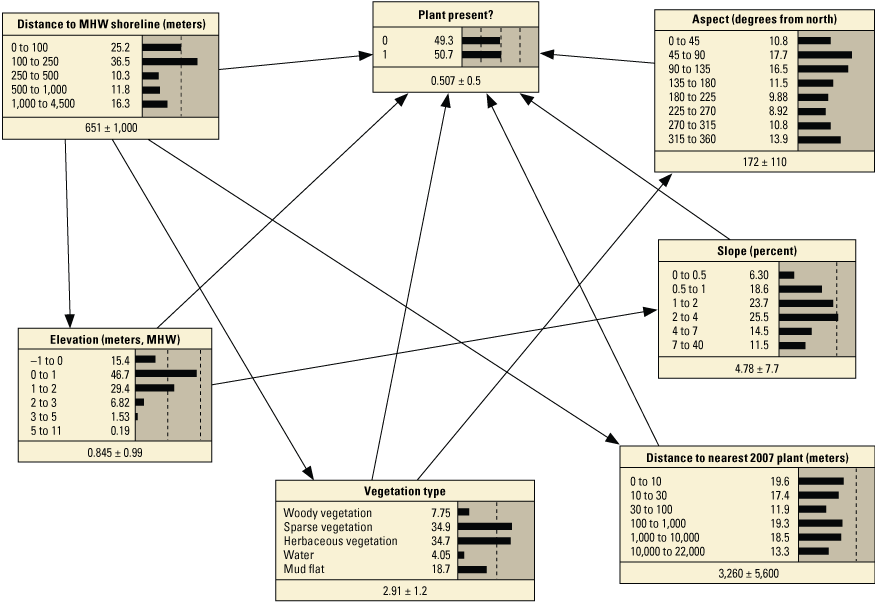
Bayesian network (BN) for point model (PM) 18: BN trained using data from 2008. Dashed vertical lines indicate 25, 50, and 75 percent. MHW, mean high water.
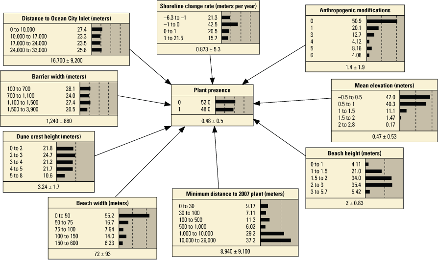
Bayesian network (BN) for transect model (T) 3: BN trained using data from 2008 and 2014. Dashed vertical lines indicate 25, 50, and 75 percent.
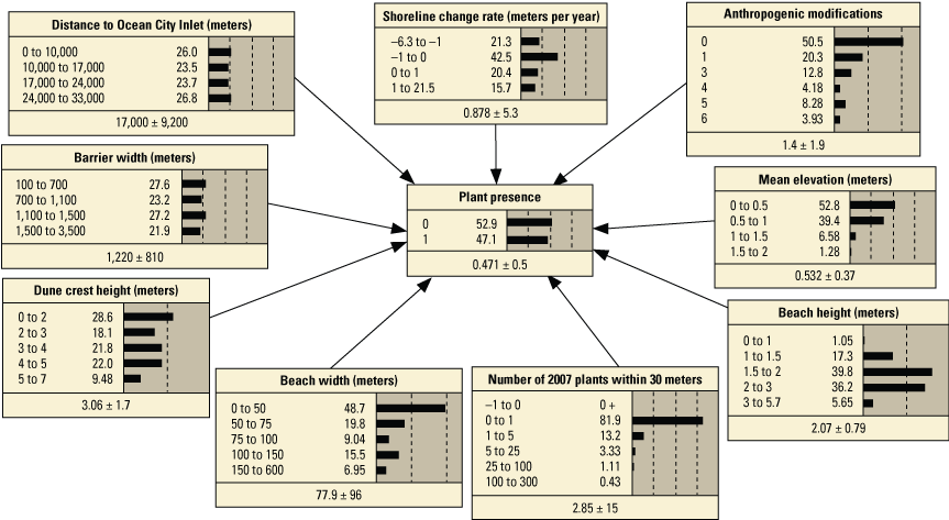
Bayesian network (BN) for transect model (T) 5: BN trained using data from 2008 and 2014. Dashed vertical lines indicate 25, 50, and 75 percent.
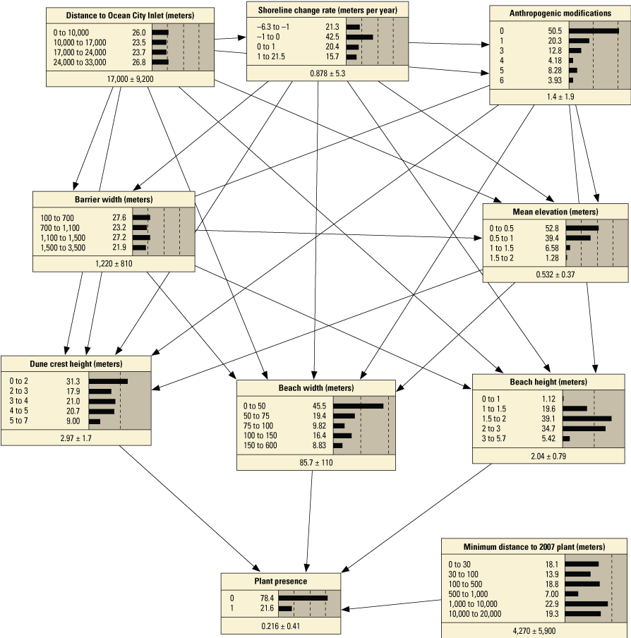
Bayesian network (BN) for transect model (T) 9: BN trained using data from 2008 and 2014. Dashed vertical lines indicate 25, 50, and 75 percent.
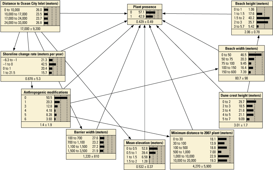
Bayesian network (BN) for transect model (T) 15: BN trained using data from 2008. Dashed vertical lines indicate 25, 50, and 75 percent.
1.2. Bayesian Network Initial Performance Scores and Hindcast Evaluation
For initial model selection, we calculated performance scores for each of the BNs and compared the percentage of habitat predicted for regions of low (kilometer marker [KM] 12) and high (KMs 24–25) SBA occurrence at Assateague Island (tables 1.3–1.6). These allowed us to compare model performance between BNs.
Table 1.3.
Initial performance test scores for Bayesian network point models using Assateague Island data collected in 2008 and 2014.[Bold entries specify scoring metrics for PM4, the Bayesian network used for the cross-validation hindcast evaluation. Shaded region specifies “structured” Bayesian networks (PM7–PM12) to distinguish them from the “simple” (PM1–PM6) and “TAN” Bayesian networks (PM13–PM18). TAN, tree-augmented naïve Bayes algorithm; no., number; SE, standard error (Fielding and Bell, 1997); PM, point model]
Table 1.4.
Percent habitat hindcast with the point model Bayesian networks for two sections of Assateague Island where there have been no seabeach amaranth observed and where they have been abundant.[Numbers reflect percentages where P(Habitat) > 0.66/P(Habitat) > 0.9 (likely and very likely on Intergovernmental Panel on Climate Change uncertainty scale). Bold entries specify scoring metrics for PM4, the Bayesian network used for hindcast evaluation. Shaded region specifies “structured” Bayesian networks (PM7–PM12) to distinguish them from the “simple” (PM1–PM6) and “TAN” Bayesian networks (PM13–PM18). TAN, tree-augmented naïve Bayes algorithm; >, greater than; BN, Bayesian network; KM, kilometer marker; PM, point model]
Table 1.5.
Initial performance test scores for Assateague Island transect model Bayesian networks.[Shaded region specifies “structured” Bayesian networks (T7–T12) to distinguish them from the “simple” (T1–T6) and “TAN” Bayesian networks (T13–T18). TAN, tree-augmented naïve Bayes algorithm; no., number; SE, standard error (Fielding and Bell, 1997); T, transect]
Table 1.6.
Percent habitat hindcast with transect model Bayesian networks for two sections of Assateague Island where there have been no seabeach amaranth observed and where they have been abundant.[Numbers reflect percentages where P(Habitat) > 0.66/P(Habitat) > 0.9 (likely and very likely on Intergovernmental Panel on Climate Change uncertainty scale). Shaded region specifies “structured” BNs (T7–T12) to distinguish them from the “simple” (T1–T6) and “TAN” networks (T13–T18). >, greater than; TAN, tree-augmented naïve Bayes algorithm; BN, Bayesian network; KM, kilometer marker; T, transect]
References Cited
Fielding, A.H., and Bell, J.F., 1997, A review of methods for the assessment of prediction errors in conservation presence/absence models: Environmental Conservation, v. 24, no. 1, p. 38–49, accessed May 11, 2021, at https://doi.org/10.1017/S0376892997000088.
Friedman, N., Geiger, D., and Goldszmidt, M., 1997, Bayesian network classifiers: Machine Learning, v. 29, no. 2, p. 131–163, accessed August 14, 2012, at https://doi.org/10.1023/A:1007465528199.
Datum
Vertical coordinate information is referenced to the local mean high water (MHW).
Horizontal coordinate information is referenced to the North American Datum of 1983 (NAD 83).
Altitude, as used in this report, refers to distance above the vertical datum.
Abbreviations
ASIS
Assateague Island National Seashore
BN
Bayesian network
DNR
Maryland Department of Natural Resources
GPS
global positioning system
IPCC
Intergovernmental Panel on Climate Change
KM
kilometer marker
KS
Kolmogorov-Smirnov test
lidar
light detection and ranging
MDA
Maryland Department of Agriculture
NPS
National Park Service
OSV
over-sand vehicle [zone]
P
probability
PM
point model
SBA
seabeach amaranth
SPI
standardized precipitation index
T
transect model
TAN
tree-augmented naïve Bayes
USFWS
U.S. Fish and Wildlife Service
USGS
U.S. Geological Survey
For more information about this report, contact:
Director, Woods Hole Coastal and Marine Science Center
U.S. Geological Survey
384 Woods Hole Road
Quissett Campus
Woods Hole, MA 02543-1598
(508) 548–8700 or (508) 457–2200
WHSC_science_director@usgs.gov
or visit our website at
Suggested Citation
Gutierrez, B.T., and Lentz, E.E., 2023, Developing a habitat model to support management of threatened seabeach amaranth (Amaranthus pumilus) at Assateague Island National Seashore, Maryland and Virginia: U.S. Geological Survey Scientific Investigations Report 2023–5034, 62 p., https://doi.org/10.3133/sir20235034.
ISSN: 2328-0328 (online)
Study Area
| Publication type | Report |
|---|---|
| Publication Subtype | USGS Numbered Series |
| Title | Developing a habitat model to support management of threatened seabeach amaranth (Amaranthus pumilus) at Assateague Island National Seashore, Maryland and Virginia |
| Series title | Scientific Investigations Report |
| Series number | 2023-5034 |
| DOI | 10.3133/sir20235034 |
| Year Published | 2023 |
| Language | English |
| Publisher | U.S. Geological Survey |
| Publisher location | Reston, VA |
| Contributing office(s) | Woods Hole Coastal and Marine Science Center |
| Description | Report: viii, 62 p.; 2 Data Releases |
| Country | United States |
| State | Maryland, Virginia |
| Other Geospatial | Assateague Island National Seashore |
| Online Only (Y/N) | Y |
| Additional Online Files (Y/N) | N |
| Google Analytic Metrics | Metrics page |