

Preliminary Machine Learning Models of Manganese and 1,4-Dioxane in Groundwater on Long Island, New York
Links
- Document: Report (5.93 MB pdf) , HTML , XML
- Data Release: USGS data release - Data and model archive for preliminary machine learning models of manganese and 1,4-dioxane in groundwater on Long Island, New York
- Download citation as: RIS | Dublin Core
Acknowledgments
The author thanks the Suffolk County Water Authority for providing water-quality data. Also appreciated are the contributions of many U.S. Geological Survey colleagues involved in water-quality sampling and data compilation for the National Water Quality Program (formerly, the National Water-Quality Assessment [NAWQA] Program), as well as the reviews and assistance with this study provided by Paul Stackelberg, Shawn Fisher, and Christopher Schubert, U.S. Geological Survey.
Abstract
Manganese and 1,4-dioxane in groundwater underlying Long Island, New York, were modeled with machine learning methods to demonstrate the use of these methods for mapping contaminants in groundwater in the Long Island aquifer system. XGBoost, a gradient boosted, ensemble tree method, was applied to data from 910 wells for manganese and 553 wells for 1,4-dioxane. Explanatory variables included soil properties, groundwater flow, land use, and other features that describe the hydrogeology and geochemistry of the aquifer system. Four models were developed to predict the probability of manganese concentrations greater than a detection level of 10 micrograms per liter (µg/L) and greater than three threshold concentrations (50, 150, and 300 µg/L) relevant to drinking-water quality. One model was developed to predict the probability of 1,4-dioxane concentrations greater than a detection level of 0.07 µg/L. The 1,4-dioxane model was limited geographically to Suffolk County because of data availability. Predictions were made for two layers in the upper glacial aquifer and three layers in the Magothy aquifer, which are the upper two of the three major aquifers of the Long Island aquifer system.
The objective of the study described in this report was to demonstrate the application of the methods rather than to develop precise estimates of manganese or 1,4-dioxane concentrations at any given location. The predictive models developed in the study are considered preliminary in the sense that they are an initial effort at developing these kinds of models specifically for Long Island. The models could be improved by the inclusion of additional data, by the use of methods to improve the modeling of infrequent high concentrations of manganese and 1,4-dioxane (above threshold concentrations), and by including more explanatory variables that specifically describe conditions and contaminant sources on Long Island. Nonetheless, the distribution of model predictions and the influence of explanatory variables in the models were consistent with the expected relations between contaminant concentrations and groundwater-flow-system characteristics and the distribution of manmade sources.
Mapped predictions indicated that manganese detections were more probable in the upper glacial aquifer and along the southern shore of Long Island, consistent with the distribution of anoxic conditions in groundwater in the Long Island aquifer system. Manganese was infrequently predicted at concentrations greater than thresholds of concern for drinking-water quality in any of the aquifer layers. Detections of 1,4-dioxane were predicted in the western, more highly developed parts of Suffolk County, in the upper glacial aquifer and the top and middle layers of the Magothy aquifer, and in northwestern Suffolk County in the bottom layer of the Magothy aquifer. Although preliminary in nature and based on limited data, these mapped predictions can be used to generally identify areas where manganese and 1,4-dioxane may be present at concentrations of concern to prioritize areas for future monitoring and to guide future modeling and mapping efforts.
Introduction
Groundwater is the sole source of drinking water for 2.9 million people on Long Island, New York (fig. 1; U.S. Census Bureau, 2021). More than 1,200 public supply wells and about 45,000 domestic wells withdraw groundwater from the underlying Long Island aquifer system (Suffolk County Government, 2015; Long Island Commission for Aquifer Protection, 2019a). Permeable, sandy, and largely unconfined sediments form high-yield aquifers that are the source of this drinking water. However, these characteristics of the aquifers also make groundwater sources of drinking water on Long Island particularly susceptible to contamination.
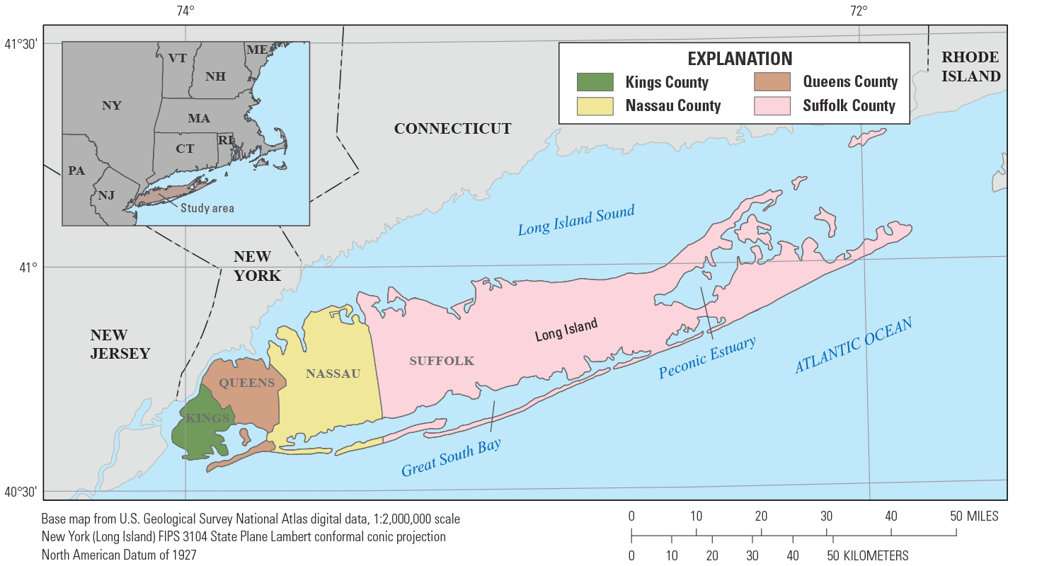
Map showing the study area of Long Island, New York, and its counties.
Groundwater contamination on Long Island is a regional and complex problem (Watson and others, 2018; Long Island Commission for Aquifer Protection, 2019a). Contaminant sources associated with human activities are distributed across the landscape in the same areas in which supply wells are located. These sources include stormwater runoff, onsite sewage disposal systems, leaks and spills from commercial and industrial activities, and fertilizer and pesticide applications (Kimmel, 1984; Long Island Commission for Aquifer Protection, 2019a). Excessive nitrogen loads and the presence of volatile organic compounds (VOCs), pesticides, and other synthetic organic compounds are of concern and have been detected in drinking-water supplies (Eckhardt and Stackelberg, 1995; Phillips and others, 2015; Long Island Commission for Aquifer Protection, 2019a; Misut and others, 2020; Fisher and others, 2021). Excessive nitrogen also is a concern in groundwater discharge, which delivers the accumulated loads from upgradient point and non-point sources to streams, ponds, and sensitive coastal waters such as Long Island Sound, Peconic Estuary, and Great South Bay (fig. 1). Additionally, because groundwater travel times from sources to discharge can be tens or hundreds of years long, contaminants released today and decades in the past will be of concern for many years to come.
Many agencies, organizations, and programs collect and analyze data on groundwater quality in the aquifer system underlying Long Island. Water suppliers monitor their drinking-water sources for compliance with the Federal Safe Drinking Water Act (Public Law 93–523, 88 Stat. 1660). The Suffolk County Department of Health Services offers water-quality testing for residents who own private (domestic) wells (Suffolk County Government, 2021). Federal, State, Tribal, and county agencies [including the New York State Departments of Health and Environmental Conservation, the Nassau County Health Department, the Suffolk County Department of Health Services, the U.S. Geological Survey (USGS), the U.S. Environmental Protection Agency (EPA), and the Shinnecock Environmental Department] support or conduct groundwater quality monitoring, which sometimes includes broad suites of constituents (Long Island Commission for Aquifer Protection, 2019a). Academic researchers also collect and compile groundwater quality data (for example, Stony Brook University, 2021). Monitoring is conducted at individual contamination sites for investigative and regulatory purposes and to support possible remediation. All these efforts have resulted in a large amount of data to describe water quality at well sampling point locations within the Long Island aquifer system (Long Island Commission for Aquifer Protection, 2021).
Maps of contaminant occurrence can help water resource managers and the public to better understand the risks posed to drinking-water supplies by contaminants in groundwater. However, maps depicting point data have limitations for use in regional water-resource assessments, especially for uses in which data are spatially aggregated, such as contaminant load estimates or statistical summaries by area. Even with many data points available across a region, it is difficult to interpolate between sampling points, especially in three dimensions. These difficulties result because of the heterogeneity of sources, aquifer characteristics, groundwater-flow patterns, and subsurface chemical and biological processes. Extrapolation to unsampled areas may need to rely on relations of concentrations with coarsely scaled spatial proxies for contaminant sources, such as land use for manmade contaminants or geologic map formations for geogenic contaminants (chemicals from soils, rock, aquifer materials). For display and public education, regional-scale maps of point data (such as those showing contaminant concentrations) also can be difficult to interpret when data are dense and symbols overlap, although scalable interactive maps such as the collaborative WaterTraq application can address this problem (Long Island Commission for Aquifer Protection, 2021). Averaging across areas, such as towns or counties, also can be unsatisfying because this approach smooths out variations across large areas and maps may contain artificially sharp boundaries (Ryker, 2001).
Machine learning methods, when applied to point sample data from wells and relevant explanatory data, can produce models and maps that depict the three-dimensional distribution of contaminants in groundwater based on patterns learned from the data and thus are well suited for regional contaminant assessments. These methods have been successfully applied to map nitrate, arsenic, manganese, and salinity at the regional or national scale in the United States and elsewhere (Rodriguez-Galiano and others, 2014; Ransom and others, 2017; Rosecrans and others, 2017; Erickson and others, 2018, 2021; Sajedi-Hosseini and others, 2018; Knoll and others, 2019; Knierim and others, 2020; Pennino and others, 2020; Sahour and others, 2020). Machine learning methods work well to model contaminant occurrence in complex environments because these methods do not require that sources or underlying processes (for example, advective flow or chemical reactions) be known or explicitly specified in order to make accurate predictions. Rather than starting with a known or assumed set of relations between predictors and the simulated response variable, such as are incorporated within mathematical or physically based models, machine learning methods build models by learning the relations between predictors and response variables from the actual data (Elith and others, 2008). Additionally, the methods can accommodate complex, non-linear relations between the simulated contaminant and the explanatory variables and require no assumptions about the underlying statistical distributions of contaminant concentrations (Elith and others, 2008; Kuhn and Johnson, 2013). However, machine learning methods require large amounts of data that adequately represent the conditions in the target environment. In addition, the explanatory variables must be available throughout the areas for which predictions are made, when the models are used to predict and map contaminant concentrations across a study area.
In the study described here, the USGS developed preliminary models to predict manganese and 1,4-dioxane concentrations in groundwater in the Long Island aquifer system as an initial demonstration of the use of machine learning methods to model and map the quality of groundwater in this aquifer system. The large amount of monitoring data and the extensive past and present studies of the aquifer system (U.S. Geological Survey, 2021b) make Long Island an ideal location to apply these methods. This study was conducted as part of the USGS National Water-Quality Assessment (NAWQA) Program (more recently [2022] known as the National Water Quality Program) in conjunction with modeling and mapping groundwater quality in the Northern Atlantic Coastal Plain (NACP) regional aquifer system, in part using readily available data compiled for that regional study (DeSimone and others, 2020; DeSimone and Ransom, 2021). The NACP aquifer system is one of the principal aquifers of the United States and extends along the eastern coast from North Carolina to Long Island. Manganese, dissolved oxygen, and pH were modelled and mapped in three dimensions for the entire NACP, including the parts of the aquifer system underlying Long Island, as part of the NAWQA program.
Manganese and 1,4-dioxane were selected for modeling on Long Island as representative geogenic and manmade contaminants of current concern for drinking-water quality. Manganese is both a nuisance contaminant and a potential health concern in drinking-water sources. As a nuisance contaminant, manganese degrades water quality by causing an unpleasant taste and color, by staining laundry and plumbing, and by accumulating in distribution systems (World Health Organization, 2017). The EPA has established a non-regulatory secondary maximum contaminant level (SMCL) of 50 micrograms per liter (µg/L) as a guideline for manganese concentration in public water supplies. Manganese in drinking water also is an emerging health concern because of its potential neurological effects, especially in children (Ljung and Vahter, 2007; Björklund and others, 2017). The EPA lifetime health advisory for manganese concentration in public water supplies is 300 µg/L. Manganese is common in geologic materials and is present in Long Island aquifer system sediments as oxide coatings on grain surfaces (Walter, 1997). Manganese solubility is controlled by pH and redox conditions; therefore, the presence of manganese dissolved in groundwater depends, largely, on geochemical conditions within the aquifer system. On Long Island, manganese dissolved in groundwater sometimes requires treatment in both public supply and domestic wells (Suffolk County Government, 2015; Long Island Commission for Aquifer Protection, 2019a, Suffolk County Water Authority, 2021). Manganese also has been measured at elevated concentrations in groundwater downgradient of composting facilities on Long Island (Suffolk County Department of Health Services, 2016).
1,4-Dioxane is a synthetic organic compound of emerging concern for drinking-water supplies on Long Island and nationally (Stepien and others, 2014; U.S. Environmental Protection Agency, 2017; Long Island Commission for Aquifer Protection, 2019a). In 2020, New York State established a maximum contaminant level (MCL) of 1 µg/L for 1,4-dioxane in public water supplies, and the compound has been on the EPA contaminant candidate list since 2009 (U.S. Environmental Protection Agency, 2009, 2021; New York State Department of Health, 2020). The compound is considered a likely carcinogen (Agency for Toxic Substances and Disease Registry, 2012). 1,4-Dioxane was used as a stabilizer for solvents, such as 1,1,1-trichloroethane (TCA), and is detected in groundwater associated with contamination by TCA and other chlorinated solvents (U.S. Environmental Protection Agency, 2017). 1,4-Dioxane is present in many commercial, industrial, and consumer products including cleaning and personal care products, antifreeze, paint strippers, and waxes, and also is used in manufacturing. 1,4-Dioxane is mobile and persistent in groundwater because it is hydrophilic (having a tendency to mix with, dissolve in, or be wetted by water) and is not readily sorbed or biodegraded; 1,4-dioxane contamination also is expensive and difficult to treat in public supply systems. Detections of 1,4-dioxane are widespread in public supply wells on Long Island (Long Island Commission for Aquifer Protection, 2019b).
Purpose and Scope
This report documents the development and use of machine learning methods to model and map manganese and 1,4-dioxane in groundwater underlying Long Island. The models were developed to investigate the use of machine learning methods with available data to characterize the occurrence and distribution of contaminants in groundwater within the Long Island aquifer system. The models are considered preliminary in the sense that they are an initial effort at developing these kinds of models specifically for Long Island. The models were based on only a selected fraction of the available data that potentially could be used for these purposes, in terms of both concentration data in water from wells and explanatory variables relevant to Long Island groundwater quality. The models provide an initial depiction of predictions for the selected contaminants in groundwater underlying Long Island. Four models were developed for manganese, predicting the probability of detection and of concentrations exceeding three thresholds relevant for drinking-water quality. The models for manganese extend across the entire Long Island area. One model was developed for 1,4-dioxane, predicting the probability of detection. The 1,4-dioxane model is limited geographically to Suffolk County (fig. 1), because 1,4-dioxane data were available only for that area in this study. Similarly, the models are limited to the upper glacial and Magothy aquifers of the Long Island aquifer system because limited data were available for the deeper Lloyd aquifer. The models also represent discrete snapshots in time, based on the temporal distribution of water-quality data. For manganese, the time period represented is a 20-year period centered on 2010, whereas for 1,4-dioxane, only 2018 is represented.
This report describes data compilation, explanatory variable processing, model development and evaluation, and model applications to make predictions across the study area. Predictions concerning manganese and 1,4-dioxane concentrations were made at a 500-square-foot (ft2) resolution for five depth horizons within the Long Island aquifer system, of which three are shown in this report (all predictions are provided in DeSimone, 2023). Thus, the predictions depict the three-dimensional distribution of manganese and 1,4-dioxane in the aquifer system. Model limitations also are discussed, including suggestions for model improvement by the inclusion of additional data and testing.
Study Area
Long Island extends eastwards from the southernmost tip of New York State, roughly parallel to the Connecticut coast (fig. 1). Long Island is about 1,400 square miles (mi2) in area and 120 miles (mi) long, with a maximum width of about 23 mi. The island is bounded by Long Island Sound to the north and the Atlantic Ocean on the south and east, and it is divided politically into four counties. Kings and Queens Counties, at the western end, are boroughs of New York City and contain nearly two-thirds of the island’s total population of 8 million (U.S. Census Bureau, 2021). These counties use drinking water provided by the New York City supply system from reservoirs in upstate New York. Nassau and Suffolk Counties, which occupy most of the land area of the island, rely on public or domestic wells located on the island to supply their combined population of 2.9 million (U.S. Census Bureau, 2021). More than 400 million gallons per day (Mgal/d) are pumped from public supply wells, and an additional 15 Mgal/d is withdrawn by domestic (private household) wells, on an average annual basis (Kenny and others, 2009; Long Island Commission for Aquifer Protection, 2019a).
Land use and population density generally vary from west to east on Long Island along a gradient of decreasing development. High- and medium-intensity developed land use occupies most of Kings and Queens Counties (fig. 2; U.S. Geological Survey, 2021a, b). Nassau County contains mostly medium-to-low intensity developed land use and developed open space, along with some high-intensity developed, forest, and other undeveloped land uses/land cover. Land use in Suffolk County varies from high-, medium-, and low-intensity developed land use and developed open space in the west to forest, agriculture, and predominantly low-intensity developed land use/land cover in the east. Population density ranged from less than 1,000 people per hectare in parts of Suffolk and Nassau Counties to more than 16,000 people per hectare in parts of Kings and Queens Counties in 2010 (Falcone, 2016).
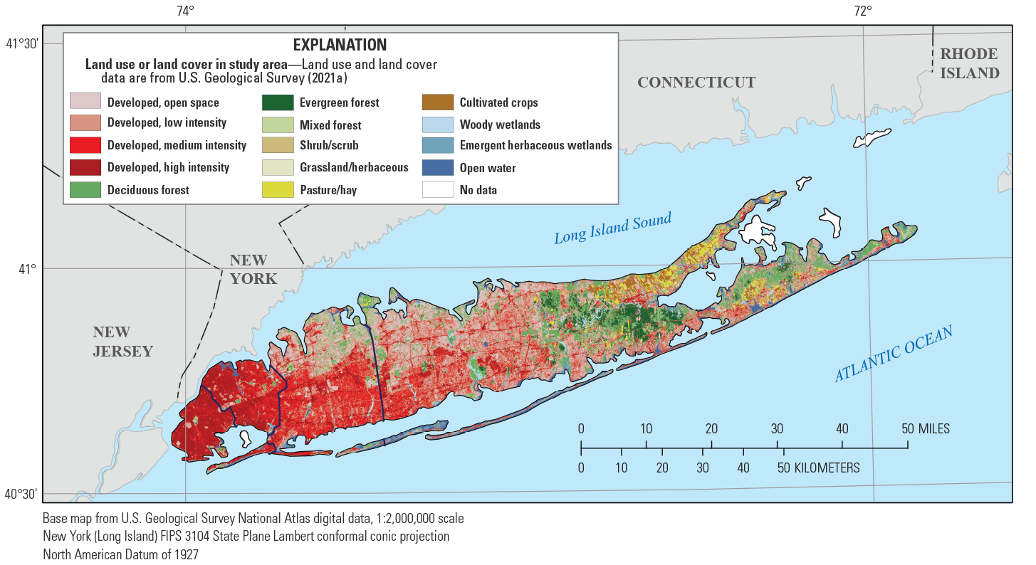
Map showing land use and land cover on Long Island, New York.
The aquifer system underlying Long Island is predominantly composed of glaciofluvial, glaciolacustrine, deltaic, and morainal sediments of Pleistocene and Cretaceous age, which form a seaward thickening wedge over crystalline bedrock and reach a total thickness of nearly 2,000 feet (ft; Walter and others, 2020b). The upper glacial aquifer and the Magothy aquifer and its associated aquifers (Monmouth greensand and Jameco aquifer, collectively referred to as the “Magothy aquifer” in this report) are the primary sources of drinking water supplies on Long Island (fig. 3). The low-permeability Gardiners Clay, which is of limited areal extent, separates the upper glacial and Magothy aquifer mainly along the southern shore of Long Island. The Lloyd aquifer, not included this study, underlies the Magothy aquifer and is separated from the Magothy aquifer by the Raritan confining unit (Walter and others, 2020b). Lithologically, the aquifer system sediments range from coarse-grained sand and gravel to silt and clay. Glacial moraines, composed of more poorly sorted and less permeable sediments than the fluvial and deltaic deposits, extend in an east-west trending band on the northern half of the island and into the two forks on the eastern end (Walter and Finkelstein, 2020; Walter and others, 2020b). Lignite, a low-grade coal, is common as interstitial particles and as interbedded layers and lenses in the middle parts of the Magothy aquifer (Walter and Finkelstein, 2020).
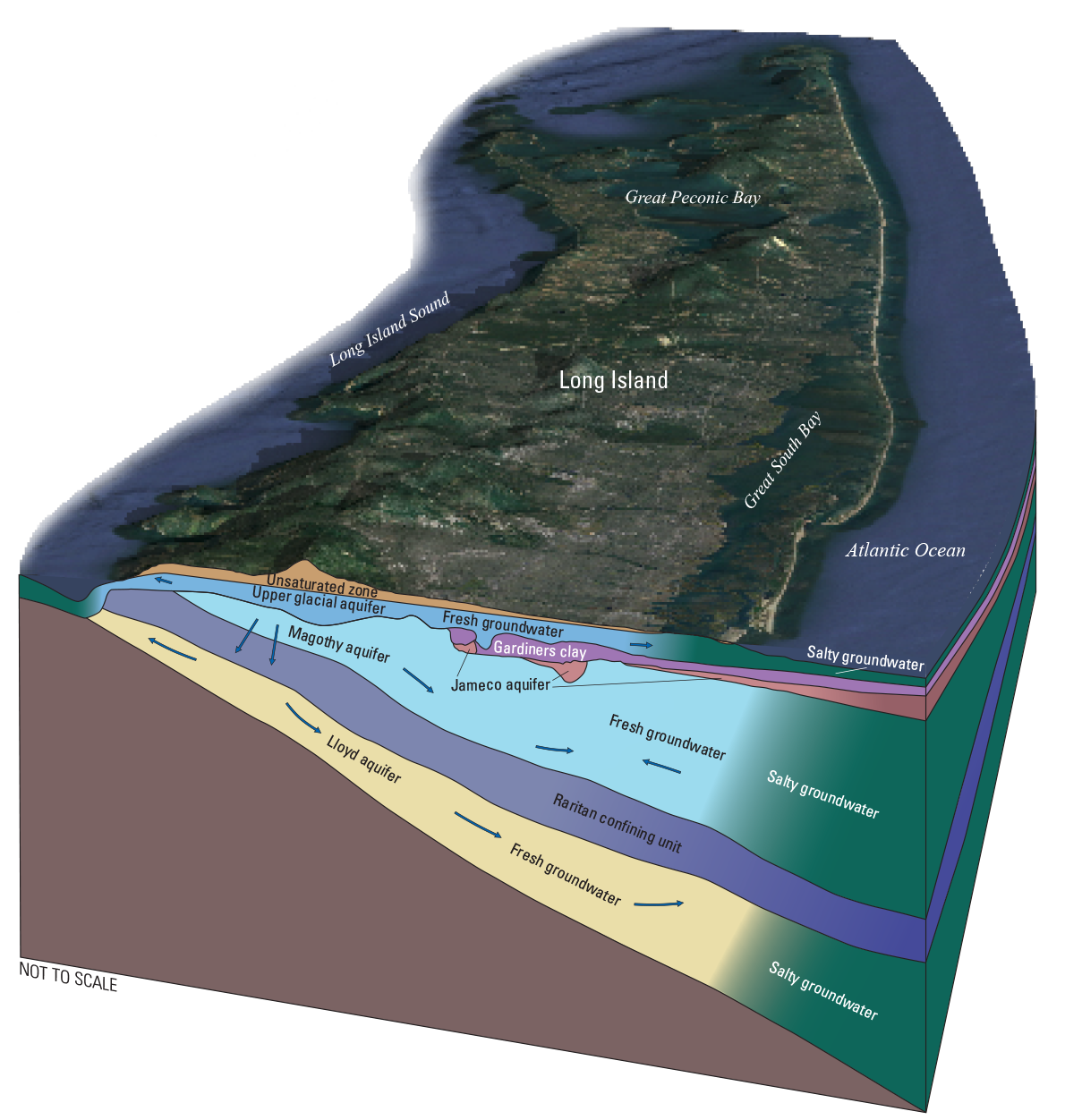
Three-dimensional schematic diagram showing major aquifers and confining units and general directions of groundwater flow on Long Island, New York. Modified from Walter and others (2020b).
In the upper glacial aquifer, groundwater is recharged across the landscape from precipitation and groundwater flow is towards freshwater streams and the coasts (fig. 3). A regional groundwater divide extends in the east-west direction along the center of the island. The Magothy and Lloyd aquifers are recharged by downward vertical flow in bands along this groundwater divide, which represent about one-quarter of the island area for recharge to the Magothy aquifer and only about 1 percent of the island area for recharge to the Lloyd aquifer (Walter and others, 2020b). Groundwater in the upper glacial aquifer is generally young (less than 25 years residence time), except near the shore where flow is upward from the Magothy aquifer to discharge; groundwater in the Magothy aquifer is generally tens to hundreds of years old; and groundwater in the Lloyd aquifer is generally thousands of years old, based on groundwater-flow model simulations (Buxton and Modica, 1992). In the vertical dimension, the freshwater aquifers are bounded by salty groundwater (fig. 3); pumping has moved the saltwater interface inland along in parts of Kings and Queens Counties and along the southwestern shore of the Nassau and Suffolk Counties (Stumm and others, 2020).
Data Compilation
Manganese and 1,4-Dioxane Concentrations
Data on manganese and 1,4-dioxane concentrations in groundwater underlying Long Island consisted of well-sample data from the USGS National Water Information System (NWIS) database, the U.S. Environmental Protection Agency (EPA) Safe Drinking Water Information (SDWIS) database, and the Suffolk County Water Authority (SCWA). The NWIS and SDWIS data were compiled as part of a national data aggregation by the USGS, in support of multiple water-quality investigations of the NAWQA program (Erickson and others, 2019). A total of 910 samples were used for manganese models (fig. 4A). Most of the manganese data (66 percent) were from the SCWA, and the remaining data were equally from NWIS and SDWIS (17 percent each). Manganese data extended across all of Long Island (fig. 4A). A total of 553 well samples were used for 1,4-dioxane, all located in Suffolk County and all from the SCWA (fig. 4B). The samples were primarily from public supply wells; the manganese data also included about 10 percent samples from monitoring wells and about 1 percent samples from supply wells of other types, including domestic wells. Both manganese and 1,4-dioxane data were denser in the western part of the island than in the east, reflecting the distribution of public supply wells across the island.
All manganese and 1,4-dioxane data were from samples representing individual wells and were of untreated groundwater. Sample collection dates for manganese data ranged from 1999 to 2018; however, only 10 samples were collected prior to 2008 and 60 percent (including all SCWA samples) were collected in 2010. All samples for 1,4-dioxane were collected in 2018. Samples for manganese were analyzed primarily by inductively coupled plasma-mass spectrometry (EPA method 200.8 or USGS method PLM43; U.S. Environmental Protection Agency, 1994a; Faires, 1992) and secondarily by inductively coupled plasma-atomic emission spectrometry (EPA method 200.7 or USGS method PLA11, U.S. Environmental Protection Agency, 1994b; Fishman, 1993). Analytical method information was not available for SDWIS samples for manganese. All samples for 1,4-dioxane were analyzed by solid-phase extraction and gas chromatograph/mass spectrometry (EPA method 522; Munch and Grimmett, 2008). Quality-control data specific to the manganese or 1,4-dioxane analytical data were not reviewed as part of this study. Manganese analysis was conducted on filtered samples for SCWA and NWIS data and on whole-water (unfiltered) samples for SDWIS; inclusion of unfiltered analysis for SDWIS data introduced an additional source of variability into the manganese dataset but this variability was considered acceptable in order to increase the sample size. Analysis for 1,4-dioxane samples was conducted on whole water (unfiltered) samples.
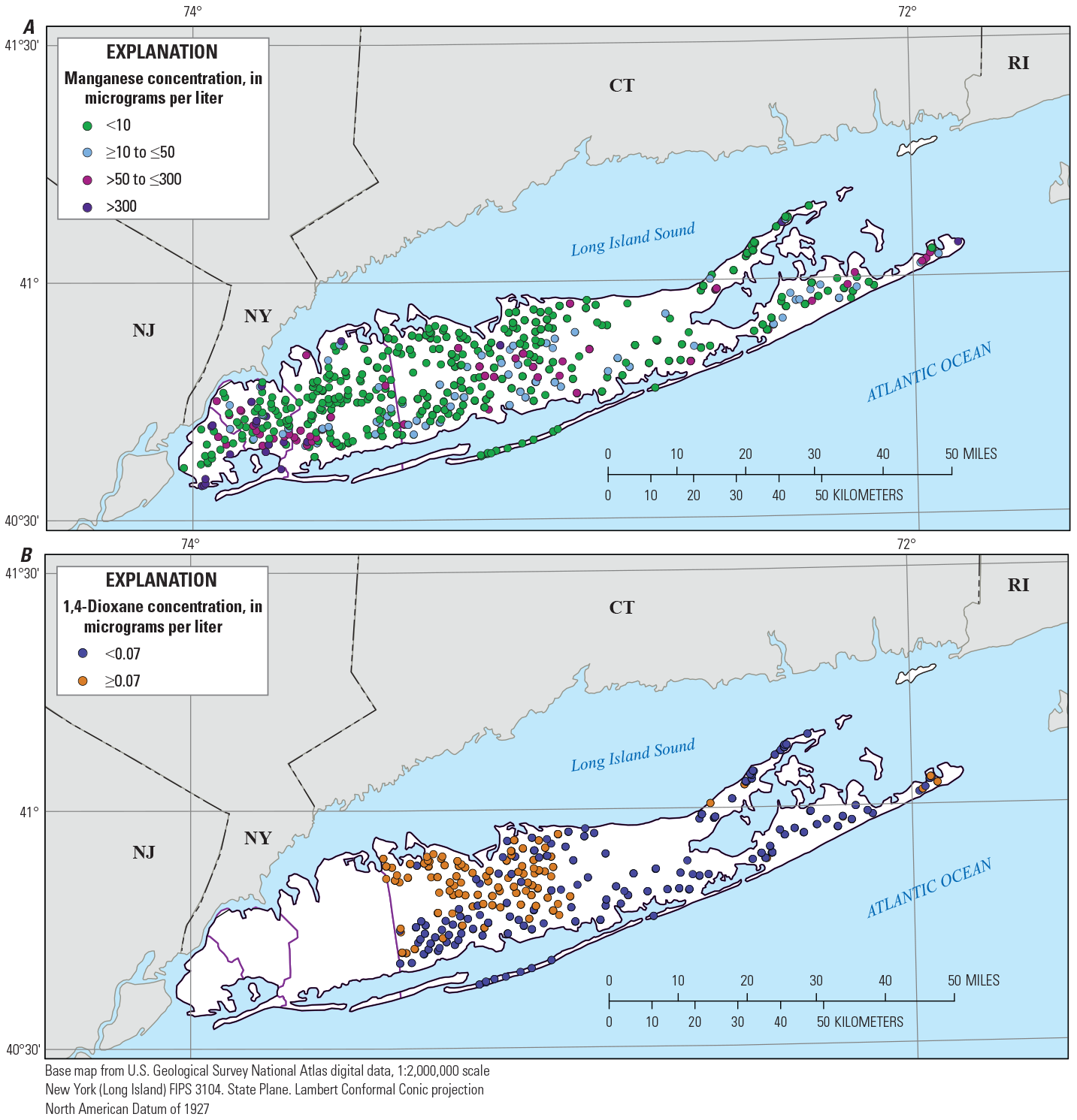
Maps showing concentrations of A, manganese and B, 1,4-dioxane in groundwater from wells in the dataset used to build the machine learning models, Long Island, New York. <, less than; >, greater than; ≥, greater than or equal to; ≤, less than or equal to.
Prediction Points
The points at which predictions were made for manganese and 1,4-dioxane across the study area corresponded spatially to the central locations of the Long Island groundwater-flow model grid of Walter and others (2020a, b). This model has a three-dimensional grid of 500-×500-ft cell size in the horizontal dimension, rotated 18 degrees counterclockwise with respect to north, and 25 layers of variable thickness in the vertical dimension. Layering in the vertical dimension reflects the dimensions of the aquifer and confining unit layers (Walter and others, 2020b). Predictions were made for the land surface area of Long Island (excluding several small islands in Queens and Suffolk counties) plus a 1.24-mi buffer area at five depth horizons that correspond to 5 of the 25 model layers: the shallow upper glacial aquifer (flow model grid layer 1), the deep upper glacial aquifer (layer 3), the top of the Magothy aquifer (layer 5), the middle of the Magothy aquifer (layer 14), and the bottom of the Magothy aquifer (layer 23). Prediction points were the vertical midpoints of the model grid layers. For the uppermost model layer (layer 1), the simulated water table rather than the layer top (which was set equal to the land surface) was used to determine the layer midpoint to use for predictions. For the upper glacial aquifer (layers 1 and 3), the depth horizons at which the predictions are made are relatively flat lying but vary in altitude; for the Magothy aquifer (layers 5, 14, and 23), the depth horizons of predictions slope downwards towards the southern coast (Walter and others, 2020b, fig. 20). For mapping, prediction points were converted to raster data layers using a raster representation of the flow model grid.
Explanatory Variables
Thirty-two explanatory variables were provided as input to the machine learning models (table 1). The variables described position on the landscape with respect to surface-water flow, position in the groundwater-flow system, groundwater recharge and flow, aquifer characteristics, the predicted geochemical conditions of pH and low dissolved oxygen, land-surface and water-table altitudes, land use, soil characteristics, population density, and the presence or absence of public water supply and sewers. Variables that represented surface characteristics, such as land use, were the same for all depths at single horizontal location. Variables that represented subsurface characteristics, such as aquifer texture variables or pH, varied with depth. Categorical information, such the presence or absence of public water, were described by binary variables indicting true or false. The variables, their sources, and the methods used to attribute them to wells or prediction points are described in the following sections.
Table 1.
Explanatory variables used in developing machine learning models for Long Island, New York.| Variable name | Variable description | Type | Source |
|---|---|---|---|
| AquiferGrp.GLA | Vertical location is in the upper glacial aquifer, binary variable | Subsurface | This study |
| AquiferGrp.MAG | Vertical location is in the Magothy aquifer, binary variable | Subsurface | This study |
| Confined.YES | Aquifer is confined at location, binary variable | Subsurface | Walter and others (2020a, b) |
| CuThkover | Thickness of overlying confining units, in feet | Subsurface | Walter and others (2020a, b) |
| DissOxy_lt1 | Predicted probability of dissolved oxygen less than 1 milligram per liter | Subsurface | DeSimone and others (2020), DeSimone and Pope (2020) |
| GwAge_median | Median simulated groundwater residence time, in years | Subsurface | DeSimone and Pope (2020), Pope and others (2020) |
| GWFlux_thkwtd | Thickness-weighted, simulated groundwater flux, in square feet per day | Subsurface | Walter and others (2020a, b) |
| Land_surface | Altitude of the land surface, in feet above North American Vertical Datum of 1988 | Surface | Walter and others (2020a, b) |
| LandUse_Ag | Agricultural land use, percentage of area surrounding well | Surface | Falcone (2015) |
| LandUse_Resi | Residential land use, percentage of area surrounding well | Surface | Falcone (2015) |
| LandUse_Undev | Undeveloped land use, percentage of area surrounding well | Surface | Falcone (2015) |
| LandUse_Urban | Urban land use, percentage of area surrounding well | Surface | Falcone (2015) |
| Lignite_mean | Probability of lignite presence in aquifer sediments | Subsurface | Finkelstein and Walter (2020), Walter and Finkelstein (2020) |
| Magothy_RechA.YES | Location within recharge area of the Magothy aquifer, binary variable | Surface | Walter and others (2020b) |
| MOHP_DSD1 | Multiorder hydrologic position variable DSD1, in meters | Surface | Belitz and others (2019); Moore and others (2019) |
| MOHP_LP2 | Multiorder hydrologic position variable LP2, dimensionless | Surface | Belitz and others (2019); Moore and others (2019) |
| pH | Predicted pH | Subsurface | DeSimone and others (2020), DeSimone and Pope (2020) |
| PopDens | Population density, mean in area surrounding well, people per hectare | Surface | Falcone (2016) |
| Pyrite_mean | Probability of pyrite presence in aquifer sediments | Subsurface | Finkelstein and Walter (2020), Walter and Finkelstein (2020) |
| Recharge | Recharge from a soil-water balance model, in feet per day | Surface | Walter and others (2020a, b) |
| Sewer_PrivW.PWS | Public water supply is present at location, binary variable | Surface | Walter and others (2020a, b) |
| Sewer_PrivW.PVW | Private water supply is present at location, binary variable | Surface | Walter and others (2020a, b) |
| Sewer_PrivW.SEW | Sewering is present at location, binary variable | Surface | Walter and others (2020a, b) |
| SiltClay_mean | Probability of clay presence in aquifer sediments | Subsurface | Finkelstein and Walter (2020), Walter and Finkelstein (2020) |
| Soil_ClayPct | Soil percent clay, mean in area surrounding well | Surface | Wieczorek (2014) |
| Soil_Hydric | Soil percent hydric soils, mean in area surrounding well | Surface | Wieczorek (2014) |
| Soil_OrgMat | Soil organic matter content, mean percent in area surrounding well | Surface | Wieczorek (2014) |
| Soil_SandPct | Soil percent sand, mean in area surrounding well | Surface | Wieczorek (2014) |
| Soil_SiltPct | Soil percent silt, mean in area surrounding well | Surface | Wieczorek (2014) |
| Soil_WatCap | Soil available water capacity, mean in area surrounding well, in centimeters per centimeter | Surface | Wieczorek (2014) |
| WaterTable | Altitude of the simulated water table, in feet above North American Vertical Datum of 1988 | Surface | Walter and others (2020a, b) |
| Well_depth | Depth of the well or prediction point (vertical location), in feet below land surface | Subsurface | This study |
Surface Variables
Explanatory variables representing soil characteristics, land use, and population density were attributed to well and prediction point locations as area-weighted averages within 1,640-ft circular buffer areas surrounding the point locations. Soil characteristics were calculated as area- and depth-weighted averages of Soil Survey Geographic database (SSURGO) variables compiled by Wieczorek (2014). Land-use variables were derived from a national data layer (NAWQA wall-to-wall anthropogenic land use trends [NWALT]) compiled by Falcone (2015). The 19 land uses of the NWALT database were combined into four explanatory variables as follows. Agricultural combined categories of crops (land-use class 43), pasture/hay (class 44), and grazing potential (class 45). Residential combined categories of recreation (class 24), high density residential (class 25), low-medium density residential (class 26), and developed, other (class 27). Undeveloped combined the semi-developed categories of urban interface, high (class 31), urban interface, low-medium (class 32), and anthropogenic (manmade), other (class 33) with the categories of mining/extraction (class 41), timber and forest cutting (class 42), low use (class 50), and very low use, conservation (class 60). Urban combined categories of major transportation (class 21), commercial/services (class 22), and industrial/military (class 23). The combined results from 2002 and 2012 land use data layers were averaged to form the final four explanatory variables. Population density was derived from the 2010 data layer compiled by Falcone (2016).
Land-surface altitude, water-table altitude, recharge, and the presence of public water supply or sewers were from the data compiled for, or simulated by, the groundwater-flow model of Walter and others (2020a, b) representing average 2005–15 conditions. These variables were attributed to well and prediction point locations by intersecting the point locations with a geographic information system (GIS) data layer of the flow model grid. Variables were set equal to the values of the grid cells in which the points were located. The land-surface altitude was equal to the top of the uppermost layer of flow model, which is the land surface derived from light detection and ranging (lidar) data (Westenbroek and others, 2010; Walter and others, 2020b). Recharge is derived from a soil-water balance model, and the values of this variable were the unadjusted values prior to model calibration. The variable describing location within the recharge area of the Magothy aquifer was also based on groundwater flow simulations, but represents the predevelopment conditions, as shown in Walter and others (2020b, fig. 33).
Explanatory variables describing position on the land surface with respect to streams and their watersheds include two multiorder hydrologic position (MOHP) variables determined from Belitz and others (2019) and Moore and others (2019). These variables describe the distance between streams and their watershed divides (DSD variables) and the relative lateral position between streams and their divides (LP variables) for each location in a watershed, for streams of orders 1 (headwater streams) to 9 (large rivers). DSD1 and LP2 were selected for use in this study from among possible MOHP variables, based on visual inspection of their variation across Long Island. The MOHP variables were attributed to well and prediction point locations by intersecting the point locations with the MOHP raster GIS data layers (Moore and others, 2019).
Subsurface Variables
Subsurface explanatory variables were attributed to well locations based on the vertical location of the well screen. Where well screen information was not available, well screen bottom altitude was set equal to well depth, and well screen top altitude was estimated by assuming a well screen length of 60 ft, which was about the average well screen length for public supply wells in the dataset used in this study. For prediction points, subsurface variables were attributed to points based on the depth or altitude of the prediction point; for variables derived from the groundwater-flow model, values were directly assigned based on the flow model grid layer corresponding to the prediction point. The well-depth variable was set equal to the depth of the prediction point below land surface.
The aquifer in which a well or prediction point was located, the presence of overlying confining units, and the thickness of overlying confining units was determined using the Long Island aquifer system hydrogeologic framework as depicted in the dimensions of the flow model grid (Walter and others, 2020a, b). For wells with screen altitude data that would have placed them in flow model grid zones simulated as confining units or moraine (14 wells or 1.5 percent of the total number of wells), variables based on the flow model grid were designated as missing. Thickness-weighted, simulated groundwater flux was calculated by summing cell-by-cell inflows for the simulated 2005–15 period and dividing by cell thickness; for the topmost model layer (layer 1), cell thickness was based on the simulated water table and the bottom of layer 1. In cases where well screens extended across more than one model layer within the same aquifer, values of thickness-weighted, simulated groundwater flux for the layers at the well location intersected by the screen were averaged. For prediction points, which were only located within a single model layer by design, the value of thickness-weighted, simulated groundwater flux was set equal to the value for the layer, as previously described.
The explanatory variables representing the probability of clay, lignite, and pyrite in aquifer sediments were derived from the three-dimensional texture model of the upper glacial and Magothy aquifers underlying Long Island as described by Finkelstein and Walter (2020) and Walter and Finkelstein (2020). These variables were included because the presence of clay, lignite, and pyrite potentially affect geochemical conditions in the aquifer sediments where these materials are present. Lignite, a low-grade coal, and pyrite, an iron sulfide mineral, are reducing agents and, when chemically weathered, cause oxygen to be depleted. Clay-rich aquifer sediments also can be associated with reducing conditions. In the horizontal dimensions, the 500-ft2 resolution grid of texture data points corresponds to the flow model grid of Walter and others (2020a, b). Thus, flow-cell location was used to identify the texture model grid cell where each well or prediction point was located. Texture model values, which are spaced vertically at 10-ft depth intervals, were averaged within the top and bottom of well screen altitudes to determine these explanatory variables for most wells. For some short-screened (less than 10 ft) wells, the well screen fell between texture model values; these wells were assigned the texture model values vertically closest to the well screen top or bottom altitude. Prediction points, which were single altitude values, similarly were assigned the texture model value closest in altitude to the prediction point.
pH and the probability of low dissolved oxygen (dissolved oxygen concentration less than 1 mg/L) were from 1-square-kilometer (km2 [0.4-mi2]) resolution predictions for the regional NACP aquifer system from machine learning models (DeSimone and Pope, 2020; DeSimone and others, 2020). pH and the probability of low dissolved oxygen were included because these variables describe aquifer geochemistry and are particularly important for manganese solubility and sorption. The median simulated groundwater residence time was derived from values calculated as input to the regional NACP pH and dissolved oxygen machine learning models (DeSimone and Pope, 2020), which were based on data in Pope and others (2020). Groundwater residence time is a potentially important variable for both manmade and geogenic contaminants. Younger water is more likely to have been affected by land-surface activities, and concentrations of geogenic contaminants can change along flow paths as groundwater quality evolves through reaction with aquifer sediments. In the NACP model datasets, each regional aquifer is represented by a single value, so that there was one value each for the surficial (the upper glacial) and the Magothy aquifers. Well and prediction point locations were intersected with a GIS data layer of the regional NACP prediction grid. Variable values of pH, the probability of low dissolved oxygen, and median simulated groundwater residence time were set equal to the values of the 1-km2 regional grid cell and the regional aquifer where the well or prediction point was located.
Machine Learning Modeling Methods
The XGBoost method was used to fit machine learning models to the manganese and 1,4-dioxane concentration data. XGBoost is a gradient boosting, ensemble tree method in which predictive models are built from many simple decision trees (Friedman, 2001; Elith and others, 2008; Chen and Guestrin, 2016). Decision trees are added sequentially in model building and each new tree is fit to the residuals of the previous predictions. XGBoost uses stochastic gradient boosting, which builds each tree on a random subset of the data, thereby increasing model robustness, and includes regularization terms to counteract data overfitting (Friedman, 2002; Chen and Guestrin, 2016). Overfitting occurs when a model is so closely constructed to fit the training data that it does not generalize well to new data.
Models were developed to predict the probability of concentrations greater than threshold concentration values for both manganese and 1,4-dioxane. For manganese, four models were developed, predicting the probability of (1) detection, represented by a threshold of 10 µg/L, (2) concentrations exceeding the SMCL of 50 µg/L, (3) concentrations exceeding 150 µg/L, which is one-half the EPA lifetime health advisory, and (4) concentrations exceeding the health advisory of 300 µg/L (U.S. Environmental Protection Agency, 2018). For 1,4-dioxane, one model was developed to predict the probability of detection, represented by a threshold of 0.07 µg/L.
XGBoost was implemented in the R computing environment (version 3.6.3; R Core Team, 2021) using the R packages xgboost (version 1.1.1.1; Chen and others, 2020) and caret (classification and regression training, version 6.0–86; Kuhn, 2019). Modeling was performed on the USGS Tallgrass supercomputer (U.S. Geological Survey, 2021c). The XGBoost algorithm was run to generate tree-based models (general parameter booster equal to “gbtree”) and the loss function was specified for binary classification (learning parameter objective equal to “binary:logistic”). Hyperparameters (XGBoost booster parameters) were determined using a grid search. A large grid (7,776 total combinations) including multiple values for each hyperparameter was tested. Seven hyperparameters were adjusted: nrounds, the maximum number of iterations; eta, which controls the learning rate or the contribution of each subsequent tree; max_depth, the maximum allowed tree depth; min_child_weight, the minimum number of instances (observations) allowed in a tree leaf; col_subsample_bytree, the proportion of total features used to construct each tree; subsample, the proportion of the total training data observations used to build each tree; and gamma, a regularization parameter (Chen and others, 2020). The range of values in the grid were as follows: nrounds, from 100 to 700 (varying by 100); eta, from 0.005 to 0.2 (5 values); max_depth, from 3 to 9 (varying by 2); min_child_weight, from 3 to 9 (varying by 3); colsample_bytree, from 0.5 to 0.9 (varying by 0.2); subsample, from 0.5 to 0.9 (varying by 2); and gamma, from 0 to 1 (varying by 1).
XGBoost hyperparameters were selected using tenfold cross validation, implemented in the caret package, and applied to training subsets of the well data. The manganese and 1,4-dioxane well datasets were divided into training (80 percent of the data) and testing (20 percent) subsets for each of the five models using the createDataPartition function of the caret package. This function divides datasets in such a way that the relative proportions of observations within user-specified classes is maintained (v. 6.0–86; Kuhn, 2019). The cross-validation process further partitions the training data subset to build models for each unique combination of hyperparameters. In tenfold cross validation, the training dataset is split into 10 subsets (folds), of which 9 are used to build the model, and the held-out 10th fold is used to evaluate the model. This splitting and model building is repeated 10 times. Model performance is quantified by averaging a selected performance metric across the 10 cross-validation holdout folds. In this study, accuracy was the performance metric selected for use in cross validation. The XGBoost hyperparameters used in the model with the highest accuracy were the selected hyperparameters.
Final machine learning models were built for the four manganese concentration thresholds and for 1,4-dioxane using the hyperparameters selected through cross validation and the complete training dataset. These final models were then tested by using them to make predictions for the 20 percent testing data subsets, which were not used in model building. Model performance metrics included the following: accuracy, the percentage of correctly predicted observations; sensitivity (also known as recall), the percentage of true positive observations predicted correctly; specificity, the percentage of true negative observations predicted correctly; kappa, a measure of agreement between observed and predicted values that accounts for the agreement that would result because of chance (Kuhn and Johnson, 2013); and a metric termed AUC, the area under the receiver operating characteristic (ROC) curve (Fawcett, 2006). All performance metrics except AUC were calculated using the confusionMatrix function of the R caret package (v. 6.0–86; Kuhn, 2019). AUC was calculated using the roc function of the pROC R package (v. 1.16.2).
Manganese and 1,4-Dioxane Concentrations in Groundwater From Wells
Manganese concentrations ranged from less than 10 µg/L to 9,000 µg/L in the dataset used to develop the machine learning models. Manganese was detected in groundwater at concentrations greater than or equal to 10 µg/L in 31.1 percent of well samples (table 2). Only 2.9 percent of concentrations were greater than the health advisory of 300 µg/L, and 12.1 percent were greater than the SMCL of 50 µg/L. Manganese concentrations in groundwater from the upper glacial aquifer were higher and exceeded the SMCL or health advisory about twice as frequently as concentrations in groundwater from the Magothy aquifer. 1,4-Dioxane was detected (concentration greater than or equal to 0.07 µg/L) in 42.0 percent of groundwater samples in the dataset used for the machine learning model, at concentrations that ranged from 0.07 to 22.3 µg/L. In contrast to detection frequencies and concentrations of manganese, detection frequencies for 1,4-dioxane in the upper glacial and Magothy aquifers were similar.
Table 2.
Well characteristics and manganese and 1,4-dioxane concentrations by aquifer in the data used to build the machine learning models, Long Island, New York.[Data are summarized from DeSimone (2023). Percentages may not sum to 100 because of rounding. ft bls, feet below land surface; µg/L, microgram per liter; %, percentage; >, greater than; <, less than; ≥, greater than or equal to; ≤, less than or equal to; —, not available]
Predictive Models of Manganese and 1,4-Dioxane
Model Selection and Performance
The final XGBoost models developed for manganese and 1,4-dioxane are described in terms of their hyperparameters in table 3 and their performance metrics in table 4. The model objects, input data, and output data are documented in DeSimone (2023). For simplicity during this preliminary study, all five final models were selected by maximizing accuracy, as described previously, during hyperparameter tuning (model training). Accuracy in this context is the proportion of correct predictions, both positive (correctly predicting a concentration above the threshold) and negative (correctly predicting a concentration below the threshold), where positive predictions are instances in which the predicted probability is greater than 0.5. Use of accuracy as the performance metric to maximize during model training is reflected in the high accuracy metrics for all five models (table 4). The high accuracy values also may indicate that the models may overfit the training data.
Table 3.
XGBoost hyperparameters used in the final models for predicting manganese and 1,4-dioxane in groundwater underlying Long Island, New York.[Data are from models documented in DeSimone (2023). XGBoost hyperparameters are defined in Chen and others (2020). Mn, manganese; >, greater than; ≥, greater than or equal to; µg/L, microgram per liter]
Table 4.
Performance metrics for training and testing data subsets of the final models for predicting manganese and 1,4-dioxane in groundwater underlying Long Island, New York.[Data are from models documented in DeSimone (2023). The data subsets contained 728 or 729 (training) and 181 or 182 (testing) samples for manganese (Mn) and 443 (training) and 110 (testing) samples for 1,4-dioxane. µg/L, microgram per liter; AUC, area under the receiver operating characteristic curve; >, greater than; > greater than or equal to]
For classification models based on datasets in which the negative instances greatly outnumber the positive instances, accuracy is an overly optimistic measure of model performance (Kuhn and Johnson, 2013). High accuracies can be achieved by simply predicting the majority class because correct prediction of the minority class, which is often of greater interest, contributes little to overall accuracy (Maloof, 2003; Sun and others, 2009). The kappa statistic is an alternative measure of the agreement between predicted and observed classes that takes into account the degree of agreement that would result because of chance (Viera and Garrett, 2005; Kuhn and Johnson, 2013). Kappa values range from 0 (no agreement) to 1 (perfect agreement). The kappa values for the testing data subsets for models were within the ranges of agreement described as follows (Viera and Garrett, 2005): substantial agreement (from 0.61 to 0.80) for the 1.4-dioxane model and moderate agreement (from 0.41 to 0.60) for the manganese models. Sensitivity is the proportion of correctly predicted positive instances (here, detections or concentrations greater than the threshold); its inverse, specificity, is the proportion of correctly predicted negative instances. In the manganese and 1,4-dioxane models, sensitivity was less than specificity for all models in both training and testing data subsets; among the manganese models, sensitivity was low for the three models predicting the probability of manganese concentrations greater than 50, 150, and 300 µg/L (table 4).
Sensitivity, specificity, kappa, and accuracy all are dependent on the probability threshold (0.5 in this study) used to classify model output into positive and negative instances. The AUC performance statistic describes the capability of a classification model to distinguish between positive and negative instances across all possible probability thresholds (James and others, 2013). AUC values are not biased towards the minority or majority class and are relatively insensitive to class imbalance (unequal data distribution among classes) except when data are highly skewed (Fawcett, 2006; Branco and others, 2016). AUC is the area under a curve that plots the true positive rate (correct classification of positive instances, the same as sensitivity) against the false positive rate (incorrectly classifying negative instances as positive) as the probability threshold for classification changes. AUC values range from 0 to 1, with a value of 1 indicating perfect capability to distinguish between positive and negative instances, a value of 0.5 indicting a capability no better than chance, and a value of 0 indicating perfect incorrect classification. AUC values for the testing data subsets ranged from 0.714 to 0.904 for manganese and AUC was 0.951 for 1,4-dioxane (table 4), indicating predictive skill relative to no-information, chance predictions.
Changing the probability threshold for identifying positive instances is one approach for addressing class imbalance in predictive models; other approaches include altering the input datasets or modeling process through oversampling, undersampling, or weighting (Maloof, 2003; Sun and others, 2009; Branco and others, 2016; Krawczyk, 2016). Altering the input datasets or modeling process to address imbalance was beyond the scope of this study. However, changing the probability threshold is a postprocessing step that can be easily applied to model output. This approach was applied to the output from manganese models at the 50, 150, and 300 µg/L concentration thresholds. Using a probability threshold of 0.3 rather than 0.5 to identify positive predicted instances increased the training data subset sensitivity to 0.977 (from 0.852) for the 50 µg/L manganese model, to 0.949 (from 0.718) for 150 µg/L model, and to 0.714 (from 0.619) for the 300 µg/L model. For the testing data subsets, sensitivity increased to 0.545 (from 0.318) for the 50 µg/L model and to 0.556 (from 0.333) for the 150 µg/L model; testing data sensitivity for the 300 µg/L model (0.400) did not change.
It is important to note, however, that the small sample size of the testing data subsets (181 or 182 samples), combined with the low frequency of positive instances, meant that the numbers of positive instances in testing data subsets for the models were small (22, 9, and 5 positive instances for the 50, 150, and 300 µg/L models, respectively). Thus, a small change in the number of positive instances correctly or incorrectly predicted results in a relatively large change in sensitivity for the models (for example, a change in the prediction of one of the five positive instances in the 300 µg/L model would change the sensitivity by 0.2). The models also have random components, both in the model-development algorithm and in the training/testing data partitioning, and this randomness also introduces instability in model-performance metrics when sample sizes are small. A conclusion from this analysis, and from the model-performance metrics for these models generally, is that a larger dataset or the use of methods to address class imbalance, such as the methods described previously, would be needed to better predict manganese concentrations for the higher concentration thresholds.
Explanatory Variables in the Models
The final models retained 23 to 31 of the 32 explanatory variables that were provided as input to the model development process. In this section, the explanatory variables that were the most important are described and their influence on model predictions is discussed. Patterns of explanatory variable importance and influence that are interpretable and consistent with prior understanding provide confidence in model predictions because this consistency indicates that the models are capturing and simulating patterns that are reflective of underlying physical, chemical, or biological processes. However, it should be noted that explanatory variables may be used as surrogates for other factors or processes that are not included in the model, or their influence may reflect interactions with other variables that are not readily discernable.
The top 10 most influential variables in each model are shown in figure 5, where influence is described by the XGBoost gain metric; gain quantifies the fractional contribution of the variable to model predictions (Chen and others, 2020). The complete listing of variables in each final model and their importance rankings are provided in appendix 1. The direction of influence of these variables is shown by partial dependence plots (PDPs; fig. 6). A PDP shows the average change in the predicted probability as a variable changes in value when all other variables in the model are held at their observed values (Greenwell, 2017). For simplicity, PDPs are shown for the top 10 ranked variables for the 1,4-dioxane model and for only one of the manganese models, the model predicting the probability of manganese concentrations greater than or equal to 10 µg/L (manganese detection). Note that PDPs do not capture interactions between variables and can be difficult to interpret when relations are complex and not monotonic, especially for lower-ranked explanatory variables.
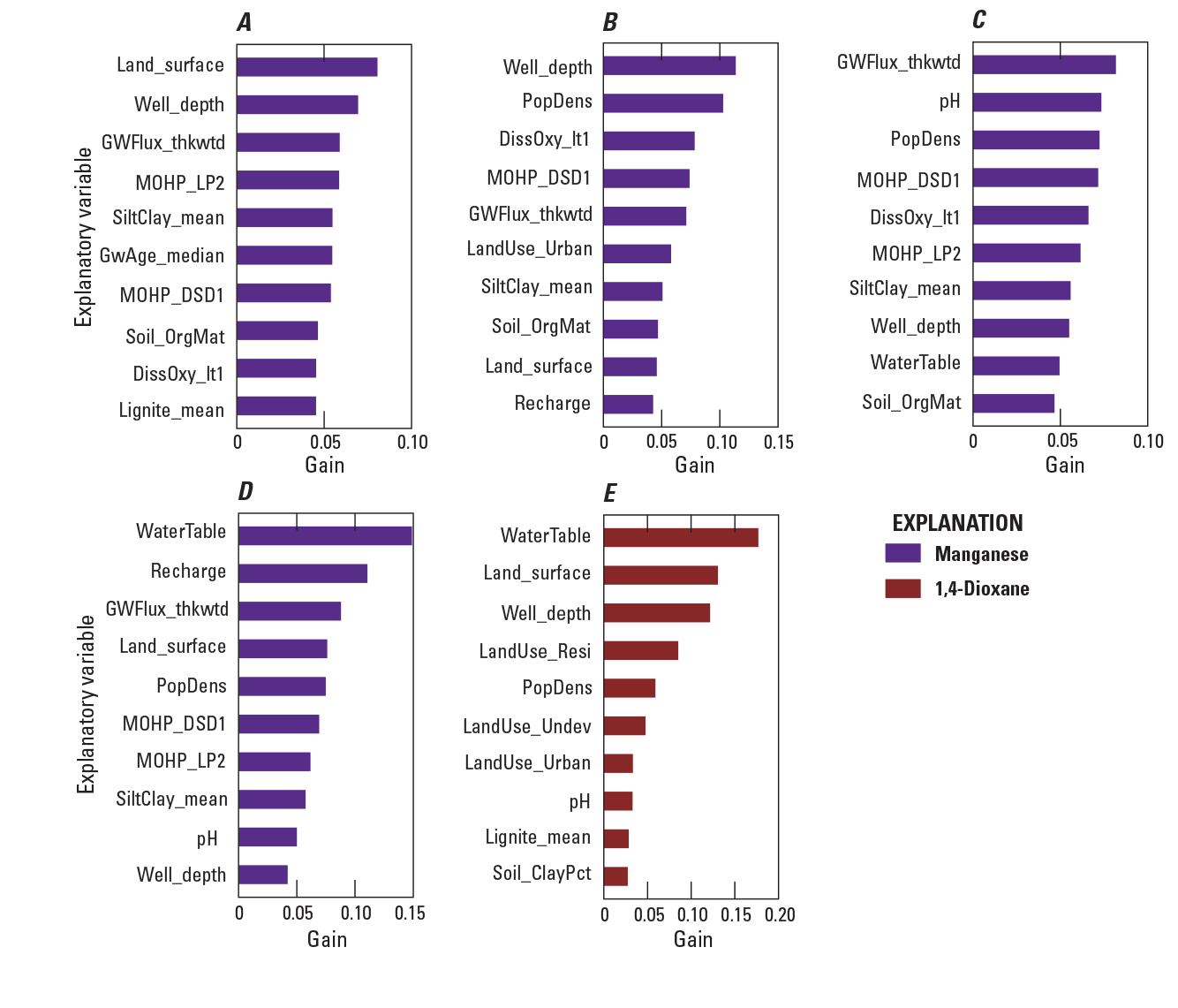
Top ten most influential explanatory variables in the manganese and 1,4-dioxane models for Long Island, New York. A, Manganese greater than or equal to 10 micrograms per liter. B, Manganese greater than 50 micrograms per liter. C, Manganese greater than 150 micrograms per liter. D, Manganese greater than 300 micrograms per liter. E, 1,4-Dioxane greater than or equal to 0.07 microgram per liter. Explanatory variable names are defined in table 1.
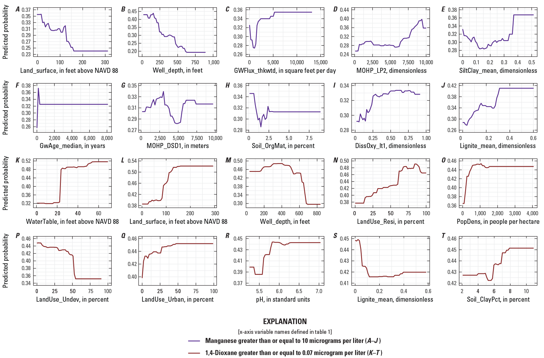
Partial dependence plots for the top ten most influential explanatory variables in the model of A–J, manganese greater than or equal to 10 micrograms per liter and K–T, 1,4-dioxane greater than or equal to 0.07 microgram per liter for Long Island, New York. Explanatory variable names are defined in table 1. NAVD 88, North American Vertical Datum of 1988.
Depth or vertical location in the Long Island aquifer system, captured by the variable Well_depth, was among the top three most important variables in all but two of the models and was among the top 10 in all models (fig. 5). The direction of influence of Well_depth also was the same in all models; the predicted probability of manganese concentrations above thresholds or 1,4-dioxane detection decreased with increasing well depth. For 1,4-dioxane, the predicted probability of detection started decreasing at a deeper depth (about 400 ft; fig. 6M), than for manganese (about 200 ft; fig. 6B), possibly reflecting the greater prevalence of 1,4-dioxane deeper in the Magothy aquifer (Long Island Commission for Aquifer Protection, 2019b) compared with manganese.
Land-surface and water-table altitudes also were among the top ranked variables in the manganese and 1,4-dioxane models (fig. 5, Land_surface and WaterTable variables). For these variables, however, the directions of influence in the manganese models and in the 1,4-dioxane model were not the same. The predicted probability of 1,4-dioxane detection was greater at higher water-table and land-surface altitudes (fig. 6K–L), whereas the predicted probability of manganese concentrations above thresholds decreased at higher land-surface altitudes, and when it was among the top 20 variables in the manganese models, at higher water-table altitudes (fig. 5A; the PDP for the WaterTable variable was not among the top 10 for the manganese model at the 10 µg/L threshold and is not shown). These relations point to the more likely presence of higher manganese concentrations in groundwater beneath low-lying areas and near the coast of Long Island, and the more likely detection of 1,4-dioxane in the central, upland areas of the island.
Some of the most important variables in the manganese models described location on the landscape with respect to surface-water flow and location within the groundwater-flow system. These include thickness-weighted, simulated groundwater flux (GWFlux_thkwtd), which was among the top five variables in all four manganese models, and the two MOHP variables (MOHP_DSD1, MOHP_LP2) that describe land-surface position with respect to streams (fig. 5A–D). The GWFlux_thkwtd and MOHP variables were not among the top 10 most influential variables in the 1,4-dioxane model. Instead, three of the four variables representing land use, LandUse_Resi, LandUse_Undev, and LandUse_Urban, were the fourth, sixth, and seventh most influential variables, respectively, in the 1,4-dioxane model (fig. 5E). In contrast, a land use variable was among the top 10 (ranked sixth) in only one of the manganese models. The contrasting importance of flow-related variables on manganese concentrations as compared to the importance of land-use variables on 1,4-dioxane detection is consistent with the primarily geogenic sources of manganese as opposed to the manmade sources of 1,4-dioxane.
The redox condition variable DissOxy_lt1, the probability of low dissolved oxygen (dissolved oxygen concentration less than 1 mg/L), was ranked ninth, third, and fifth in the three lower threshold manganese models (10, 50, and 150 µg/L, respectively) and eleventh in the 300-µg/L threshold manganese model and in the 1,4-dioxane model. Conceptually, low dissolved oxygen (anoxic redox condition) is positively associated with dissolved manganese in groundwater, because manganese is more soluble in anoxic water, and that is the direction of influence of the DissOxy_lt1 variable on the probability of manganese detection, at concentrations greater than 10 µg/L. The direction of influence of the variable in the 1,4-dioxane model was the opposite; the probability of 1,4-dioxane detection was less with increasing probability of low dissolved oxygen. This relation may reflect the less likely detection of 1,4-dioxane in old, confined groundwater that was recharged before 1,4-dioxane use that is also anoxic, rather than any direct influence of redox condition, especially if 1,4-dioxane could be degraded under aerobic conditions (Adamson and others, 2015). The influence of DissOxy_lt1, the probability of low dissolved oxygen, in the three manganese models at thresholds other than 10 µg/L, was either not monotonic (50 and 300 µg/L models) or was inversely related to the probability of manganese concentrations greater than the model threshold (150 µg/L). These complex relations may result in part because of interactions among explanatory variables that were not investigated as part of this study.
Mapped Predictions
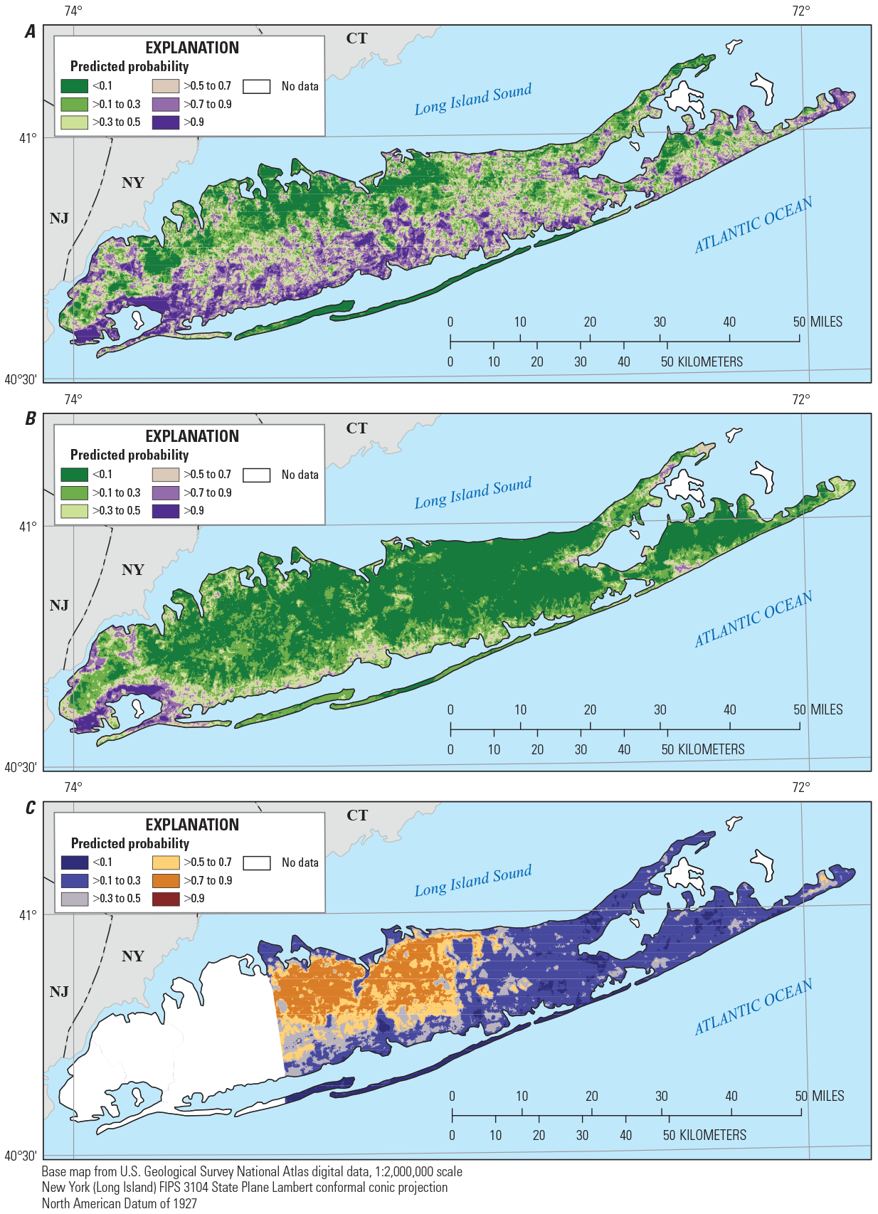
The predicted probability of manganese detected at concentrations greater than or equal to 10 µg/L, manganese concentrations greater than the SMCL of 50 µg/L, and 1,4-dioxane detected at concentrations greater than or equal to 0.07 µg/L are shown in figures 7 to 11. Predicted probabilities are shown at two depth horizons in the upper glacial aquifer (figs. 7–8), and at three depth horizons in the Magothy aquifer (top, middle, and bottom; figs. 9–11). Predictions are not shown for manganese concentrations greater than 150 and 300 µg/L thresholds because of their infrequent occurrence and the low sensitivity of the models at those thresholds. Mapped predictions are available in tagged image file format (tiff) in DeSimone (2023).
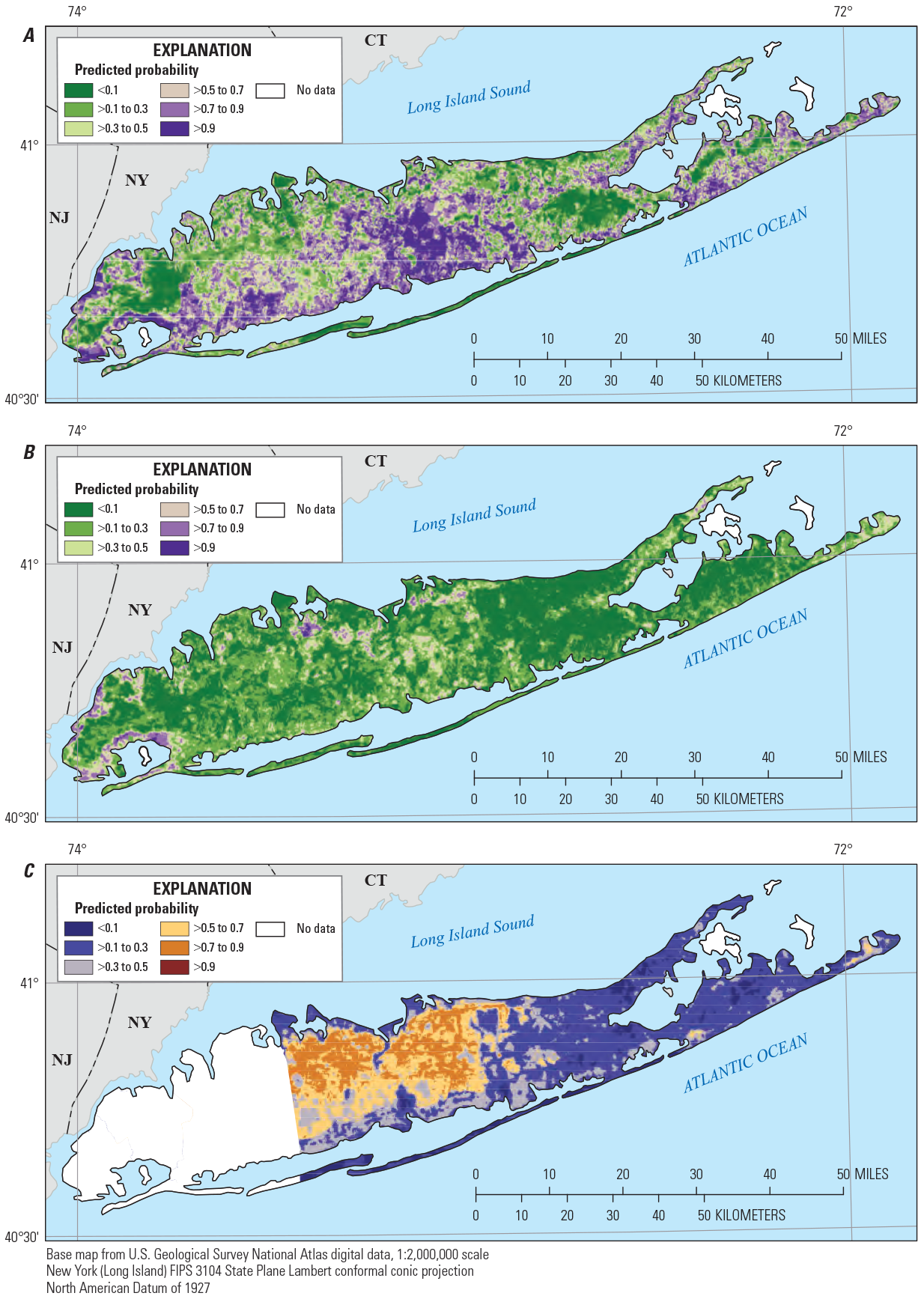
Predicted probability for the top layer of the upper glacial aquifer underlying Long Island, New York, of A, manganese concentrations greater than or equal to (≥) 10 micrograms per liter, B, manganese concentrations greater than (>) 50 micrograms per liter, and C, 1,4-dioxane concentrations ≥0.07 microgram per liter. <, less than.
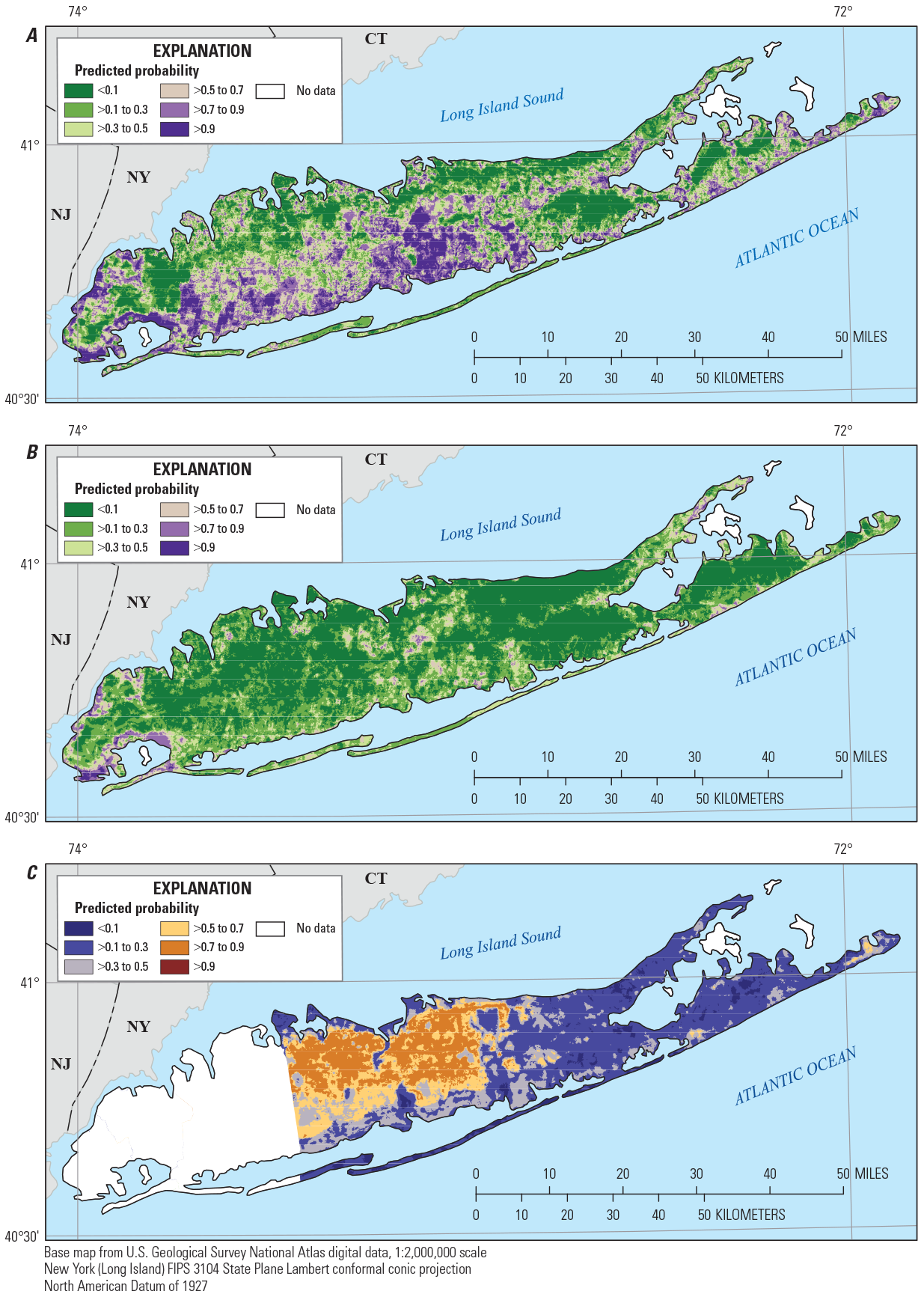
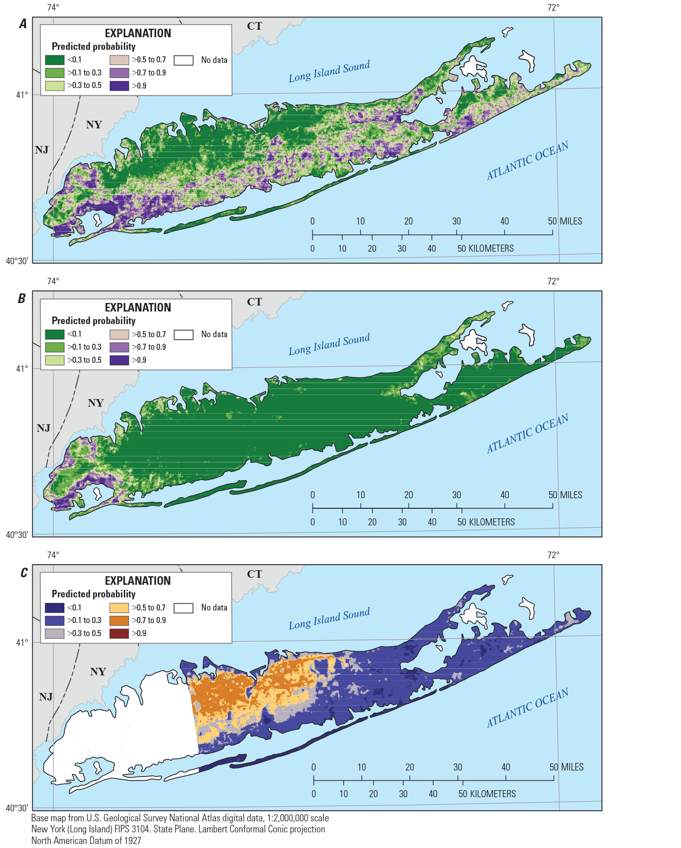
Predicted probability for the bottom layer of the upper glacial aquifer underlying Long Island, New York, of A, manganese concentrations greater than or equal to (≥) 10 micrograms per liter, B, manganese concentrations greater than (>) 50 micrograms per liter, and C, 1,4-dioxane concentrations ≥0.07 microgram per liter. <, less than.
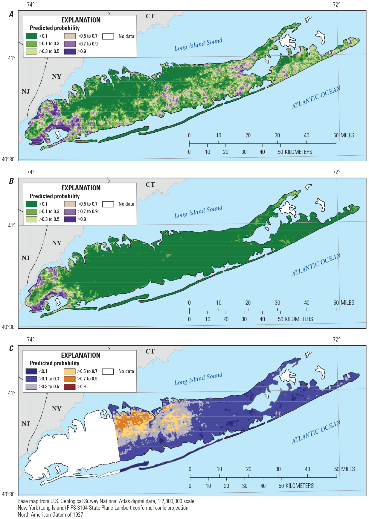
Predicted probability for the top layer of the Magothy aquifer underlying Long Island, New York, of A, manganese concentrations greater than or equal to (≥) 10 micrograms per liter, B, manganese concentrations greater than (>) 50 micrograms per liter, and C, 1,4-dioxane concentrations ≥0.07 microgram per liter. <, less than.
Predicted probability for a middle layer of the Magothy aquifer underlying Long Island, New York, of A, manganese concentrations greater than or equal to (≥) 10 micrograms per liter, B, manganese concentrations greater than (>) 50 micrograms per liter, and C, 1,4-dioxane concentrations ≥0.07 microgram per liter. <, less than.
Predicted probability for the bottom layer of the Magothy aquifer underlying Long Island, New York, of A, manganese concentrations greater than or equal to (≥) 10 micrograms per liter, B, manganese concentrations greater than (>) 50 micrograms per liter, and C, 1,4-dioxane concentrations ≥0.07 microgram per liter. <, less than.
Predicted detections of manganese (concentrations greater than or equal to 10 µg/L, probability greater than 0.5) were distributed throughout much of the top layer of the upper glacial aquifer and were predicted with higher probability along the southern shore and in the central part of the island (fig. 7). In the bottom layer of the upper glacial aquifer and in the top and middle layers of the underlying Magothy aquifer (figs. 8–10), predicted manganese detections were more limited to the southern half of the island. This distribution of manganese detections is consistent with the occurrence of groundwater in which oxygen has been depleted over long flow paths along the southern shore or through contact with reducing material such as lignite or pyrite (Brown and others, 1999; Walter and Finkelstein, 2020), and the increased solubility of manganese under reducing conditions. Manganese concentrations greater than the SMCL of 50 µg/L were predicted infrequently in any of the aquifer layers (figs. 7–11).
Detections of 1,4-dioxane (concentrations greater than or equal to 0.07 µg/L, probability greater than 0.5) were predicted across most of the western, more highly developed half of Suffolk County. The areas in which 1,4-dioxane was predicted to occur, in both the upper glacial aquifer layers and in the top and middle of the Magothy aquifer, were similar and extended from the northern shore to near the southern shore of the island in these aquifer layers (figs. 7–10). In the bottom layer of the Magothy aquifer (fig. 11), the area in which 1,4-dioxane was predicted likely to be detected was smaller and was limited to the northwestern part of Suffolk County near the northern shore.
Model Limitations
The machine learning models developed in this study are considered preliminary and their interpretations are otherwise limited for various reasons, as discussed in this section. The models developed for this study were based on a selected fraction of the data potentially available for use in modeling manganese and 1,4-dioxane concentrations in groundwater underlying Long Island. The relatively small sample size and sparse distribution of samples in some parts of the aquifer system place limits on the accuracy that the models can achieve. Class imbalance (unequal data distribution among classes) in the model training data, especially when combined with the small sample size, also limited the capability of the models to correctly predict high concentrations of manganese and 1,4-dioxane (model sensitivity). These limitations could be addressed by expanding the datasets used to build the models and by use of more sophisticated modeling methods than used here to address class imbalance. In addition, it is anticipated that additional explanatory variables, specific to Long Island, such as historical land use and improved resolution of groundwater-flow and source information, would also likely improve model accuracy, sensitivity, and overall model performance.
The degree to which model results accurately described the entire aquifer system was also potentially affected by the representativeness of the well dataset. One example of such a potential effect is the possible effect of well type. Nearly all of the concentration data used to build the models in this study were collected from public supply wells, which may shape the water-quality dataset in various ways (Suffolk County Government, 2015). Public supply wells open to unconsolidated deposits typically have long well screens (for example, more than 10 ft). Water withdrawn from a long-screened well may be a mixture of groundwater from parts of the aquifer with differing geochemical conditions. This introduces variability that may make it more difficult to predict a redox-sensitive constituent like manganese, especially when redox conditions are affected by heterogeneous aquifer sediment textures (Walter, 1997; Brown and others, 2019; Walter and Finkelstein, 2020). Additionally, the high pumping rates (for example, hundreds or thousands of gallons per minute) at some supply wells may alter flow directions so that their samples reflect water quality over a broader area and from shallower depths than samples from wells with lower pumping rates or with no active withdrawals. Expansion of the well dataset to include data from monitoring wells could provide insight into the representativeness of models built primarily on public supply well data such as those of the present study. Expanding the dataset to include monitoring wells could perhaps also fill some of the spatial gaps in sample density, especially for 1,4-dioxane, and thereby better define the conditions associated with 1,4-dioxane detection across Long Island.
Temporal variability in manganese or 1,4-dioxane concentrations was not considered extensively in developing the models described here. Constituent concentrations in groundwater are not static over time, even for constituents like manganese that originate primarily from geogenic sources (Degnan and others, 2020). Manganese concentration data were collected from a 20-year time period (1999 to 2018), over which concentrations may have varied because of changes in the groundwater-flow system, seasonal effects, or locally, manmade sources such as compositing facilities (Suffolk County Department of Health Services, 2016). 1,4-Dioxane data were all collected in 2018, but even data from a single year such as these data represent a large time period (multiple years) in source characteristics because of the varying groundwater-travel times from sources to the sampling locations. Explanatory variables that varied over time were represented by a single year, centrally located within the 20-year time period, or averaged over multiple years. For contaminants that vary over time, time averaging of explanatory variables and temporal discord between the explanatory variables and the sample data may reduce the meaningful, process-based information provided by the explanatory variables. For contaminants that vary over short time periods (for example, weeks or months), use of single point-in-time concentration data may introduce variability that cannot be accurately predicted using static, long-term-averaged explanatory variables and cannot be well characterized at the regional scale.
Finally, spatial resolution places limitations on model accuracy as well as limitations on intended model use. For example, some explanatory variables, such as predicted pH, the predicted probability of low dissolved oxygen, and simulated groundwater residence time, were obtained from regional groundwater-flow models. The spatial resolution of these variables is relatively coarse compared to the size of Long Island, and model predictions reflect the spatial resolution of the explanatory variables. Finer scale data would be more useful for the Long Island machine learning models and could increase model accuracy. Moreover, although predictions presented in this report are at a relatively fine grid cell resolution of 500 ft2, the model results are intended to represent regional patterns across Long Island rather than to predict concentrations at specific point locations.
Summary
Groundwater is the sole source of drinking water for millions of people in Long Island, New York. More than 1,200 public supply wells and about 45,000 domestic wells withdraw groundwater from the Long Island aquifer system. Permeable, sandy, and largely unconfined sediments form high-yield aquifers that are the source of this drinking water. However, these characteristics of the aquifers also make groundwater sources of drinking water on Long Island particularly susceptible to contamination. Groundwater contamination on Long Island is a regional and complex problem.
The objective of the study described here was to demonstrate the application of machine learning methods to model and map contaminants in groundwater underlying Long Island. The aquifers considered in this study consist of the upper glacial aquifer and the Magothy aquifer, which are the upper two of the three major aquifers of the Long Island aquifer system. The predictive models developed in the study are considered preliminary in the sense that they are an initial effort at developing these kinds of models specifically for Long Island. The models were based on only a selected fraction of the available data that potentially could be used for these purposes, in terms of both concentration data in water from wells and explanatory variables relevant to Long Island groundwater quality. This study was completed by the U.S. Geological Survey as part of the National Water-Quality Assessment Program (more recently known as the National Water Quality Program).
Manganese and 1,4-dioxane in groundwater underlying Long Island were modeled using machine learning methods and the resulting predictions mapped in three dimensions. The models were based on concentration data in groundwater from 910 wells for manganese and from 553 wells for 1,4-dioxane, mostly from public supply wells. Explanatory variables described soil, aquifer, and groundwater-flow characteristics, land use, the predicted pH and probability of low dissolved oxygen in groundwater, and other features of the Long Island study area. Four models were developed for manganese, predicting the probability of detection (represented by a threshold of 10 micrograms per liter [µg/L]), concentrations exceeding the secondary maximum contaminant level (SMCL) of 50 µg/L, concentrations exceeding 150 µg/L (which is one-half the U.S. Environmental Protection Agency [EPA] lifetime health advisory), and concentrations exceeding the health advisory of 300 µg/L. For 1,4-dioxane, one model was developed to predict the probability of detection, represented by a threshold of 0.07 µg/L. The model for 1,4-dioxane was limited geographically to Suffolk County, which extends across central and eastern Long Island.
The machine learning models were developed using the XGBoost algorithm, a gradient boosted, ensemble tree machine learning method, in the R computing environment. The XGBoost models were trained on 80 percent of the groundwater sample data from wells, using tenfold cross validation, and were tested using the remaining 20 percent of the data. Accuracy, as the proportion of all correctly predicted observations, both positive and negative, ranged from 0.768 to 0.983 in testing data subsets for the models. However, the manganese datasets were imbalanced, especially at the higher concentration thresholds, and accuracy is an overly optimistic performance metric for imbalanced datasets. An alternative measure, kappa, indicated significant agreement between predicted and observed values in testing data for the 1,4-dioxane model (kappa equal to 0.680) and moderate agreement for the manganese models (kappa from 0.410 to 0.565). AUC, another metric relatively insensitive to class imbalance, ranged from 0.714 to 0.951 for testing datasets for the models. Sensitivity, the proportion of correctly predicted positive instances, was relatively high (0.783) for 1,4-dioxane, moderate (0.696) for the manganese model at the 10 µg/L threshold, and low (from 0.318 to 0.400) for the other three manganese models.
The most influential explanatory variables in all five models included vertical location within the aquifer system (depth) as one of the highest ranked variables. For all models, the probability of detection or concentrations greater than modeled thresholds decreased with increasing depth. Variables that described location on the landscape with respect to surface-water flow and location within the groundwater-flow system were more influential in the manganese models, and variables representing land use were more influential in the 1,4-dioxane model, consistent with the geogenic and manmade sources, respectively, of these contaminants. Thus, patterns and directions of variable influence for these and several other variables generally were consistent with prior understanding of some of controlling factors on the occurrence and distribution of manganese and 1,4-dioxane in groundwater in the Long Island aquifer system.
Maps of the modeling results showed that the manganese detections (at concentrations greater than or equal to 10 µg/L) were predicted as more probable in the upper glacial aquifer and along the southern shore, consistent with the distribution of anoxic conditions in groundwater in the Long Island aquifer system. 1,4-Dioxane detections were predicted as more probable in the western half of Suffolk County. The area of predicted 1,4-dioxane detections in western Suffolk County extended from the north to near the southern shore in the upper glacial aquifer and in the top and middle layers of the Magothy aquifer but was more limited in extent in the bottom layer of the Magothy aquifer. The modeling results and mapped predictions can be used to illustrate the areas where these contaminants are more likely to be a concern for groundwater sources of drinking water on Long Island. Models and results could be improved by the inclusion of more data, especially at concentrations greater than the higher concentration thresholds for manganese and in deeper aquifer layers, by the use of more sophisticated modeling methods to address class imbalance, and by including more explanatory variables that specifically described hydrologic and water-quality conditions and possible contaminant sources on Long Island. The modeling results described here are considered preliminary and are intended to illustrate the application of the machine learning methods, rather than to provide precise estimates of manganese or 1,4-dioxane concentrations at specific locations on Long Island.
References Cited
Adamson, D.T, Anderson, R.H, Mahendra, S., and Newell, C.J., 2015, Evidence of 1,4-dioxane attenuation at groundwater sites contaminated with chlorinated solvents and 1,4-dioxane: Environmental Science and Technology, v. 49, no. 11, p. 6510–6518. [Also available at https://doi.org/10.1021/acs.est.5b00964.]
Agency for Toxic Substances and Disease Registry, 2012, Toxicological profile for 1,4-dioxane: Agency for Toxic Substances and Disease Registry, 295 p., accessed September 8, 2021, at https://www.ncbi.nlm.nih.gov/books/NBK153677/pdf/Bookshelf_NBK153677.pdf.
Belitz, K., Moore, R.B., Arnold, T.A, Sharpe, J., and Starn, J., 2019, Multiorder hydrologic position in the conterminous United States—A set of metrics in support of groundwater mapping at regional and national scales: Water Resources Research, v. 55, no. 12, p. 11188–11207, accessed April 19, 2022, at https://doi.org/10.1029/2019WR025908.
Björklund, G., Chartrand, M.S., and Aaseth, J., 2017, Manganese exposure and neurotoxic effects in children: Environmental Research, v. 155, p. 380–384, accessed April 19, 2022, at https://doi.org/10.1016/j.envres.2017.03.003.
Branco, P., Torgo, L., and Ribeiro, R.P., 2016, A survey of predictive modelling under imbalanced distributions: ACM Computing Surveys, v. 49, no. 2, p. 1–50. [Also available at https://doi.org/10.1145/2907070.]
Brown, C.J., Barlow, J.R.B., CravottaIII, C.A., and Lindsey, B.D., 2019, Factors affecting the occurrence of lead and manganese in untreated drinking water from the Atlantic and Gulf Coastal Plain aquifers, eastern United States—Dissolved oxygen and pH framework for evaluating risk of elevated concentrations: Applied Geochemistry, v. 101, p. 88–102, accessed April 19, 2022, at https://doi.org/10.1016/j.apgeochem.2018.10.017.
Brown, C.J., Walter, D.A., and Colabufo, S., 1999, Iron in the aquifer system of Suffolk County, New York, 1990-98: U.S. Geological Survey Water-Resources Investigations Report99–4126, 10 p. [Also available at https://doi.org/10.3133/wri994126.]
Buxton, H.T., and Modica, E., 1992, Patterns and rates of ground-water flow on Long Island, New York: Ground Water, v. 30, no. 6, p. 857–866. [Also available at https://doi.org/10.1111/j.1745-6584.1992.tb01568.x.]
Chen, T., and Guestrin, C., 2016, XGBoost—A scalable tree boosting system, in ACM SIGKDD International Conference on Knowledge Discovery and Data Mining, 22d, San Francisco, California, August 13–17, 2016, Proceedings: New York, Association for Computing Machinery, p. 785–794, accessed April 19, 2022, at https://doi.org/10.1145/2939672.2939785.
Chen, T., He., T., Benesty, M., and Guestrin, C., 2020, Package ‘xgboost’: R Foundation for Statistical Computing software release, accessed October 16, 2020, at https://cran.r-project.org/web/packages/xgboost/xgboost.pdf.
Degnan, J.R., Levitt, J.P., Erickson, M.L., Jurgens, B.C., Lindsey, B.D., and Ayotte, J.D., 2020, Time series of arsenic variability and the role of high-frequency monitoring at three water-supply wells in New Hampshire, USA: Science of the Total Environment, v. 709, article 135946, 13 p., accessed April 19, 2022, at https://doi.org/10.1016/j.scitotenv.2019.135946.
DeSimone, L.A., 2023, Data and model archive for preliminary machine learning models of manganese and 1,4-dioxane in groundwater on Long Island, New York: U.S. Geological Survey data release, at https://doi.org/10.5066/P90AT9YG.
DeSimone, L.A., and Pope, J.P., 2020, Data for models and maps of pH and dissolved oxygen in the Northern Atlantic Coastal Plain aquifer system, eastern USA: U.S. Geological Survey data release, accessed April 19, 2022, at https://doi.org/10.5066/P94DYERF.
DeSimone, L.A., and Ransom, K.M., 2021, Manganese in the Northern Atlantic Coastal Plain aquifer system, eastern USA—Modeling regional occurrence with pH, redox, and machine learning: Journal of Hydrology: Regional Studies, v. 37, article 100925, 20 p., accessed April 19, 2022, at https://doi.org/10.1016/j.ejrh.2021.100925.
DeSimone, L.A., Pope, J.P., and Ransom, K.M., 2020, Machine learning models to map pH and redox conditions in a layered aquifer system, Northern Atlantic Coastal Plain, eastern USA: Journal of Hydrology: Regional Studies, v. 30, article 100697, accessed April 19, 2022, at https://doi.org/10.1016/j.ejrh.2020.100697.
Eckhardt, D.A.V., and Stackelberg, P.E., 1995, Relation of ground-water quality to land use on Long Island, New York: Ground Water, v. 33, no. 6, p. 1019–1033. [Also available at https://doi.org/10.1111/j.1745-6584.1995.tb00047.x.]
Elith, J., Leathwick, J.R., and Hastie, T., 2008, A working guide to boosted regression trees: Journal of Animal Ecology, v. 77, no. 4, p. 802–813, accessed April 19, 2022, at https://doi.org/10.1111/j.1365-2656.2008.01390.x.
Erickson, M. L., Yager, R.M., Kauffman, L.J., and Wilson, J.T., 2019, Drinking water quality in the glacial aquifer system, northern USA: Science of the Total Environment, v. 694, article 133735, 14 p., accessed April 19, 2022, at https://doi.org/10.1016/j.scitotenv.2019.133735.
Erickson, M.L., Elliott, S.M., Christenson, C.A., and Krall, A.L., 2018, Predicting geogenic arsenic in drinking water wells in glacial aquifers, north-central USA—Accounting for depth-dependent features: Water Resources Research, v. 54, no. 12, p. 10172–10187. [Also available at https://doi.org/10.1029/2018WR023106.]
Erickson, M.S., Elliott, S.M., Brown, C.J., Stackelberg, P.E., Ransom, K.M., Reddy, J.E., and CravottaIII, C.A., 2021, Machine-learning predictions of high arsenic and high manganese at drinking water depths of the glacial aquifer system, northern continental United States: Environmental Science & Technology, v. 55, no. 9, p. 5791–5805, accessed June 14, 2022, at https://doi.org/10.1021/acs.est.0c06740.
Faires, L.M., 1992, Methods of analysis by the U.S. Geological Survey National Water Quality Laboratory—Determination of metals in water by inductively coupled plasma-mass spectrometry: U.S. Geological Survey Open-File Report92–634, 28 p. [Also available at https://doi.org/10.3133/ofr92634.]
Falcone, J.A., 2015, U.S. conterminous wall-to-wall anthropogenic land use trends (NWALT), 1974–2012: U.S. Geological Survey Data Series 948, 33 p., accessed April 19, 2022, at https://doi.org/10.3133/ds948.
Falcone, J.A., 2016, U.S. block-level population density rasters for 1990, 2000, and 2010: U.S. Geological Survey data release, accessed April 19, 2022, at https://doi.org/10.5066/F74J0C6M.
Finkelstein, J.S., and Walter, D.A., 2020, Aquifer texture data describing the Long Island aquifer system: U.S. Geological Survey data release, accessed April 19, 2022, at https://doi.org/10.5066/P954DLLC.
Fisher, I.J., Phillips, P.J., Bayraktar, B.N., Chen, S., McCarthy, B.A., and Sandstrom, M.W., 2021, Pesticides and their degradates in groundwater reflect past use and current management strategies, Long Island, New York, USA: Science of the Total Environment, v. 752, article 141895, 13 p., accessed April 19, 2022, at https://doi.org/10.1016/j.scitotenv.2020.141895.
Fishman, M.J., ed., 1993, Methods of analysis by the U.S. Geological Survey National Water Quality Laboratory—Determination of inorganic and organic constituents in water and fluvial sediments: U.S. Geological Survey Open-File Report93–125, 216 p. [Also available at https://doi.org/10.3133/ofr93125.]
Friedman, J.H., 2001, Greedy function approximation—A gradient boosting machine: Annals of Statistics, v. 29, no. 5, p. 1189–1232, accessed January 21, 2020, at https://projecteuclid.org/euclid.aos/1013203451.
Friedman, J.H., 2002, Stochastic gradient boosting: Computational Statistics and Data Analysis, v. 38, no. 4, p. 367–378. [Also available at http://dl.acm.org/doi/10.1016/S0167-9473(01)00065-2.]
Greenwell, B.M., 2017, Pdp—An R package for constructing partial dependence plots: R Journal, v. 9, no. 1, p. 421–436, accessed April 19, 2022, at https://journal.r-project.org/archive/2017/RJ-2017-016/index.html.
Kenny, J.F., Barber, N.L., Hutson, S.S., Linsey, K.S., Lovelace, J.K., and Maupin, M.A., 2009, Estimated use of water in the United States in 2005: U.S. Geological Survey Circular 1344, 52 p., accessed September 3, 2021, at https://doi.org/10.3133/cir1344.
Kimmel., G.E., 1984, Nonpoint contamination of groundwater on Long Island, New York, in National Research Council, ed., Groundwater contamination: National Academy Press, p. 134–140, accessed September 7, 2021, at https://doi.org/10.2172/6906720.
Knierim, K.J., Kingsbury. J.A., Haugh, C.J., and Ransom, K.M, 2020, Using boosted regression tree models to predict salinity in Mississippi embayment aquifers, central United States: Journal of the American Water Resources Association, v. 56, no. 6, p. 1010–1029, accessed April 18, 2022, at https://doi.org/10.1111/1752-1688.12879.
Knoll, L., Breuer, L., and Bach, M., 2019, Large scale prediction of groundwater nitrate concentrations from spatial data using machine learning: Science of the Total Environment, v. 668, p. 1317–1327, accessed June 12, 2022, at https://doi.org/10.1016/j.scitotenv.2019.03.045.
Krawczyk, B., 2016, Learning from imbalanced data—Open challenges and future directions: Progress in Artificial Intelligence, v. 5, p. 221–232, accessed April 19, 2022, at https://doi.org/10.1007/s13748-016-0094-0.
Kuhn, M., 2019, The caret package: R Foundation for Statistical Computing software, accessed September 12, 2019, at https://topepo.github.io/caret/index.html.
Ljung, K., and Vahter, M., 2007, Time to re-evaluate the guideline value for manganese in drinking water?: Environmental Health Perspectives, v. 115, no. 11, p. 1533–1538, accessed June 23, 2022, at https://doi.org/10.1289/ehp.10316.
Long Island Commission for Aquifer Protection, 2019a, Groundwater resources management plan—December 11, 2019: Long Island Commission for Aquifer Protection, 167 p., accessed September 3, 2021, at https://licaponline.com/wp-content/uploads/2020/10/SCWA-GRMP-2019.pdf.
Long Island Commission for Aquifer Protection, 2019b, State of the aquifer—2019 update: Long Island Commission for Aquifer Protection, 19 p., accessed September 8, 2021, at https://licaponline.com/wp-content/uploads/2020/08/SOTA_2019-1.pdf.
Long Island Commission for Aquifer Protection, 2021, WaterTraq: Long Island Commission for Aquifer Protection website, accessed September 7, 2021, at https://licaponline.com/watertraq.
Maloof, M.A., 2003, Learning when datasets are imbalanced and when costs are unequal and unknown, in ICML–2003 Workshop on Learning from Imbalanced Datasets II, Washington, D.C., August 21, 2003: International Conference on Machine Learning, 8 p., accessed September 15, 2021, at https://www.site.uottawa.ca/~nat/Workshop2003/maloof-icml03-wids.pdf.
Misut, P.E., Walter, D., Schubert, C., and Dressler, S., 2020, Analysis of remedial scenarios affecting plume movement through a sole-source aquifer system, southeastern Nassau County, New York: U.S. Geological Survey Scientific Investigations Report 2020–5090, 83 p., accessed June 21, 2022, at https://doi.org/10.3133/sir20205090.
Moore, R., Belitz, K., Arnold, T.L., Sharpe, J.B., and Starn, J.J., 2019, National multi order hydrologic position (MOHP) predictor data for groundwater and groundwater-quality modeling: U.S. Geological Survey data release, accessed April 19, 2022, at https://doi.org/10.5066/P9HLU4YY.
Munch, J.W., and Grimmett, P., 2008, Method 522—Determination of 1,4-dioxane in drinking water by solid-phase extraction (SPE) and gas chromatography/mass spectrometry (GC/MS) with selected ion monitoring (SIM): U.S. Environmental Protection Agency, accessed April 20, 2022, at https://cfpub.epa.gov/si/si_public_record_report.cfm?Lab=NERL&dirEntryId=199229.
New York State Department of Health, 2020, Maximum contaminant levels (MCLs): New York State Register, v. 42, no. 34, p. 6, accessed September 8, 2021, at https://dos.ny.gov/system/files/documents/2020/10/082620.pdf.
Pennino, M.J., Leibowitz, S.G., Compton, J.E., Hill, R.A., Sabo, R.D, 2020, Patterns and predictions of drinking water nitrate violations across the conterminous United States: Science of the Total Environment, v. 722, article 137661, 16 p., accessed June 23, 2022, at https://doi.org/10.1016/j.scitotenv.2020.137661.
Phillips, P.J., Schubert, C., Argue, D., Fisher, I., Furlong, E.T., Foreman, W., Gray, J., and Chalmers, A., 2015, Concentrations of hormones, pharmaceuticals, and other micropollutants in groundwater affected by septic systems in New England and New York: Science of the Total Environment, v. 512–513, p. 43–54, accessed June 22, 2022, at https://doi.org/10.1016/j.scitotenv.2014.12.067.
Pope, J.P., Masterson, J.P., DeSimone, L.A., Starn, J.J., 2020, Statistical summaries of simulated groundwater residence times for the 10 regional aquifers of the Northern Atlantic Coastal Plain aquifer system, at a 1 square-mile grid resolution: U.S. Geological Survey data release, accessed April 19, 2022, at https://doi.org/10.5066/P91F9JTO.
R Core Team, 2021, The R project for statistical computing: R Foundation for Statistical Computing website, accessed September 10, 2021, at https://www.R-project.org.
Ransom, K.M., Nolan, B.T., Traum, J.A., Faunt, C.C., Bell, A.M., Gronberg, J.M., Wheeler, D.C., Rosecrans, C.Z., Jurgens, B., Schwarz, G.E., Belitz, K., Eberts, S.M., Kourakos, G., and Harter, T., 2017, A hybrid machine learning model to predict and visualize nitrate concentration throughout the Central Valley aquifer, California, USA: Science of the Total Environment, v. 601–602, p. 1160–1172, accessed May 23, 2022, at https://doi.org/10.1016/j.scitotenv.2017.05.192.
Rodriguez-Galiano, V., Mendes, M.P., Garcia-Soldada, M.J., Chica-Olmo, M., and Ribeiro, L., 2014, Predictive modeling of groundwater nitrate pollution using random forest and multisource variables related to intrinsic and specific vulnerability—A case study in an agricultural setting (southern Spain): Science of the Total Environment, v. 476–477, p. 189–206, accessed June 2, 2022, at https://doi.org/10.1016/j.scitotenv.2014.01.001.
Rosecrans, C.Z., Nolan, B.T., and Gronberg, J.M., 2017, Prediction and visualization of redox conditions in the groundwater of Central Valley, California: Journal of Hydrology v. 546, p. 341–356, accessed June 21, 2022, at https://doi.org/10.1016/j.jhydrol.2017.01.014.
Ryker, S.J., 2001, Mapping arsenic in groundwater—A real need, but a hard problem: Geotimes web page, accessed September 8, 2021, at http://www.geotimes.org/nov01/feature_Asmap.html.
Sahour, H., Gholami, V., and Vazifedan, M, 2020, A comparative analysis of statistical and machine learning techniques for mapping the spatial distribution of groundwater salinity in a coastal aquifer: Journal of Hydrology, v. 591, article 125321, 12 p., accessed June 15, 2022, at https://doi.org/10.1016/j.jhydrol.2020.125321.
Sajedi-Hosseini, F., Malekian, A., Choubin, B., Rahmati, O., Cipullo, S., Coulon, F., and Pradhan, B., 2018, A novel machine learning-based approach for the risk assessment of nitrate groundwater contamination: Journal of Hydrology, v. 644, p. 954–962, accessed May 23, 2022, at https://doi.org/10.1016/j.scitotenv.2018.07.054.
Stepien, D.K., Diehl, P., Helm, J., Thoms, A., and Püttmann, W., 2014, Fate of 1,4-dioxane in the aquatic environment—from sewage to drinking water: Water Research, v. 48, p. 406–419. [Also available at https://doi.org/10.1016/j.watres.2013.09.057.]
Stony Brook University, 2021, Center for Clean Water Technology: Stony Brook University Center for Clean Water Technology website, accessed September 16, 2021, at https://www.stonybrook.edu/cleanwater/.
Stumm, F., Como, M.D., and Zuck, M.A., 2020, Use of time domain electromagnetic soundings and borehole electromagnetic induction logs to delineate the freshwater/saltwater interface on southwestern Long Island, New York, 2015–17: U.S. Geological Survey Open-File Report 2020–1093, 27 p., accessed June 23, 2022, at https://doi.org/10.3133/ofr20201093.
Suffolk County Department of Health Services, 2016, Investigation of the impacts to groundwater quality from compost/vegetative organic waste management facilities in Suffolk County: Suffolk County Department of Health Services, 152 p., accessed March 11, 2022, at https://static1.squarespace.com/static/58a74ddce3df282ccda2d0b4/t/58a8f1bd86e6c0c373936ce4/1487467007330/Final+SCDHS+VOWM+Investigation+Report.pdf.
Suffolk County Government, 2015, Suffolk County comprehensive water resources management plan: Suffolk County Government website, accessed September 3, 2021, at https://www.suffolkcountyny.gov/Departments/Health-Services/Environmental-Quality/Water-Resources/Comprehensive-Water-Resources-Management-Plan.
Suffolk County Government, 2021, Private well water testing program: Suffolk County Government website, accessed September 3, 2021, at https://www.suffolkcountyny.gov/Departments/Health-Services/Environmental-Quality/Water-Resources/Private-Well-Water-Testing-Program.
Suffolk County Water Authority, 2021, 2021 drinking water quality report: Suffolk County Water Authority website, accessed September 8, 2021, at https://www.scwa.com/water-quality/water-quality-reports/.
Sun, Y., Wong, A.K.C., and Kamel, M.S.2009, Classification of imbalanced data—A review: International Journal of Pattern Recognition and Artificial Intelligence, v. 23, no. 4, p. 687–719, accessed June 21, 2022, at https://doi.org/10.1142/S0218001409007326.
U.S. Census Bureau, 2021, QuickFacts, United States: U.S. Census Bureau database, accessed September 8, 2021, at https://www.census.gov/quickfacts.
U.S. Environmental Protection Agency, 1994a, Method 200.8—Determination of trace elements in waters and wastes by inductive coupled plasma-mass spectrometry (rev. 5.4): U.S. Environmental Protection Agency, 58 p., accessed April 20, 2022, at https://www.epa.gov/esam/epa-method-2008-determination-trace-elements-waters-and-wastes-inductively-coupled-plasma-mass.
U.S. Environmental Protection Agency, 1994b, Method 200.7—Determination of metals and trace elements in waters and wastes by inductive coupled plasma-atomic emission spectrometry (rev. 4.4): U.S. Environmental Protection Agency, 57 p., accessed April 20, 2022, at https://www.epa.gov/esam/method-2007-determination-metals-and-trace-elements-water-and-wastes-inductively-coupled-plasma.
U.S. Environmental Protection Agency, 2009, Drinking water contaminant list 3—Final: Federal Register, v. 74, no. 194, p. 51851–51862, accessed September 8, 2021, at https://www.govinfo.gov/content/pkg/FR-2009-10-08/pdf/E9-24287.pdf.
U.S. Environmental Protection Agency, 2017, Technical fact sheet—1,4-dioxane: U.S. Environmental Protection Agency EPA 505–F–17–011, 9 p., accessed September 8, 2021, at https://www.epa.gov/sites/default/files/2014-03/documents/ffrro_factsheet_contaminant_14-dioxane_january2014_final.pdf.
U.S. Environmental Protection Agency, 2018, 2018 edition of the drinking water standards and health advisories: U.S. Environmental Protection Agency EPA 822–F–18–001, 20 p., accessed April 19, 2022, at https://www.epa.gov/system/files/documents/2022-01/dwtable2018.pdf.
U.S. Environmental Protection Agency, 2021, Drinking water contaminant list 5—Draft: Federal Register, v. 86, no. 135, p. 37949–37972, accessed September 8, 2021, at https://www.govinfo.gov/content/pkg/FR-2021-07-19/pdf/2021-15121.pdf.
U.S. Geological Survey, 2021a, Data: Multi-Resolution Land Characteristics Consortium National Land Cover Database 2019 data, accessed September 19, 2021, at https://www.mrlc.gov/data.
U.S. Geological Survey, 2021b, State of the aquifer, Long Island, New York: U.S. Geological Survey New York Water Science Center web page, accessed September 8, 2021, at https://www.usgs.gov/centers/new-york-water-science-center/science/state-aquifer-long-island-new-york-0.
U.S. Geological Survey, 2021c, USGS tallgrass supercomputer: U.S. Geological Survey Advanced Research Computing web page, accessed September 22, 2022, at https://doi.org/10.5066/P9XE7ROJ.
Viera, A.J., and Garrett, J.M., 2005, Understanding interobserver agreement—The kappa statistic: Family Medicine, v. 37, no. 5, p. 360–363, accessed June 2, 2022, at https://pubmed.ncbi.nlm.nih.gov/15883903. [Also available at http://www1.cs.columbia.edu/~julia/courses/CS6998/Interrater_agreement.Kappa_statistic.pdf.]
Walter, D.A., 1997, Effects and distribution of iron-related well-screen encrustation and aquifer biofouling in Suffolk County, Long Island, New York: U.S. Geological Survey Water-Resources Investigations Report96–4217, 33 p. [Also available at https://doi.org/10.3133/wri964217.]
Walter, D.A., and Finkelstein, J.S., 2020, Distribution of selected hydrogeologic characteristics of the upper glacial and Magothy aquifers, Long Island, New York: U.S. Geological Survey Scientific Investigations Report 2020–5023, 21 p., accessed June 23, 2022, at https://doi.org/10.3133/sir20205023.
Walter, D.A., Masterson, J.P., Finkelstein, J.S., Monti, Jr., J., Misut, P.E., and Fienen, M.N., 2020a, MODFLOW–NWT and MODPATH6 used to simulate groundwater flow in the regional aquifer system on Long Island, New York, for pumping and recharge conditions in 2005–15: U.S. Geological Survey data release, accessed April 20, 2022, at https://doi.org/10.5066/P9KWQSEJ.
Walter, D.A., Masterson, J.P., Finkelstein, J.S., Monti, Jr., J., Misut, P.E., and Fienen, M.N., 2020b, Simulation of groundwater flow in the regional aquifer system on Long Island, New York, for pumping and recharge conditions in 2005-15: U.S. Geological Survey Scientific Investigations Report 2020–5091, 75 p., accessed April 20, 2022, at https://doi.org/10.3133/sir20205091.
Watson, E.B., Powell, E., Maher, N.P., Oczkowski, A.J., Paudel, B., Starke, A., Szura, K., and Wigand, C., 2018, Indicators of nutrient pollution in Long Island, New York, estuarine environments: Marine Environmental Research, v. 134, p. 109–120, accessed April 20, 2022, at https://doi.org/10.1016/j.marenvres.2018.01.003.
Westenbroek, S.M., Kelson, V.A., Dripps, W.R., Hunt, R.J., and Bradbury, K.R., 2010, SWB—A modified Thornthwaite-Mather soil-water-balance code for estimating groundwater recharge [revised March 14, 2012]: U.S. Geological Survey Techniques and Methods, book 6, chap. A31, 60 p., accessed March 11, 2013, at https://doi.org/10.3133/tm6A31.
Wieczorek, M.E., 2014, Area- and depth-weighted averages of selected SSURGO variables for the conterminous United States and District of Columbia: U.S. Geological Survey Data Series886, accessed April 19, 2022, at https://doi.org/10.3133/ds866.
World Health Organization, 2017, Guidelines for drinking water quality (4th ed.; incorporating the 1st addendum): Geneva, World Health Organization, UNESCO and Earthscan, 429 p., accessed April 20, 2022, at https://www.who.int/publications/i/item/9789241549950.
Appendix 1. Explanatory Variables and Ranking in the Machine Learning Models
Table 1.1.
Explanatory variables in the model of manganese greater than or equal to 10 micrograms per liter, Long Island, New York.[Explanatory variables are described in table 1 of this report]
Table 1.2.
Explanatory variables in the model of manganese greater than 50 micrograms per liter, Long Island, New York.[Explanatory variables are described in table 1 of this report]
Table 1.3.
Explanatory variables in the model of manganese greater than 150 micrograms per liter, Long Island, New York.[Explanatory variables are described in table 1 of this report]
Table 1.4.
Explanatory variables in the model of manganese greater than 300 micrograms per liter, Long Island, New York.[Explanatory variables are described in table 1 of this report]
Table 1.5.
Explanatory variables in the model of 1,4-dioxane greater than or equal to 0.07 microgram per liter, Long Island, New York.[Explanatory variables are described in table 1 of this report]
References Cited
Chen, T., and Guestrin, C., 2016, XGBoost—A scalable tree boosting system, in ACM SIGKDD International Conference on Knowledge Discovery and Data Mining, 22d, San Francisco, California, August 13–17, 2016, Proceedings: New York, Association for Computing Machinery, p. 785–794, accessed April 19, 2022, at https://doi.org/10.1145/2939672.2939785.
Chen, T., He., T., Benesty, M., and Guestrin, C., 2020, Package ‘xgboost’: R Foundation for Statistical Computing software release, accessed October 16, 2020, at https://cran.r-project.org/web/packages/xgboost/xgboost.pdf.
Datum
Vertical coordinate information is referenced to the North American Vertical Datum of 1988 (NAVD 88).
Horizontal coordinate information is referenced to the North American Datum of 1927 (NAD 27).
Altitude, as used in this report, refers to distance above the vertical datum.
Supplemental Information
Concentrations of chemical constituents in water are given in micrograms per liter (µg/L).
Abbreviations
EPA
U.S. Environmental Protection Agency
GIS
geographic information system
MOHP
multiorder hydrologic position
NACP
Northern Atlantic Coastal Plain
NAWQA
National Water-Quality Assessment Program
NWIS
National Water Information System
SCWA
Suffolk County Water Authority
SDWIS
Safe Drinking Water Information System
SMCL
secondary maximum contaminant level
USGS
U.S. Geological Survey
For more information, contact
Director, New England Water Science Center
U.S. Geological Survey
10 Bearfoot Road
Northborough, MA 01532
dc_nweng@usgs.gov
or visit our website at
https://www.usgs.gov/centers/new-england-water
Publishing support provided by the Pembroke and Reston Publishing Service Centers
Suggested Citation
DeSimone, L.A., 2023, Preliminary machine learning models of manganese and 1,4-dioxane in groundwater on Long Island, New York: U.S. Geological Survey Scientific Investigations Report 2022–5120, 34 p., https://doi.org/10.3133/sir20225120.
ISSN: 2328-0328 (online)
Study Area
| Publication type | Report |
|---|---|
| Publication Subtype | USGS Numbered Series |
| Title | Preliminary machine learning models of manganese and 1,4-dioxane in groundwater on Long Island, New York |
| Series title | Scientific Investigations Report |
| Series number | 2022-5120 |
| DOI | 10.3133/sir20225120 |
| Year Published | 2023 |
| Language | English |
| Publisher | U.S. Geological Survey |
| Publisher location | Reston, VA |
| Contributing office(s) | New England Water Science Center, Advanced Research Computing (ARC) |
| Description | Report: vii, 34 p.; Data Release |
| Country | United States |
| State | New York |
| Other Geospatial | Long Island |
| Online Only (Y/N) | Y |
| Additional Online Files (Y/N) | N |
| Google Analytic Metrics | Metrics page |