

Parameter Estimation at the Conterminous United States Scale and Streamflow Routing Enhancements for the National Hydrologic Model Infrastructure Application of the Precipitation-Runoff Modeling System (NHM-PRMS)
Links
- Document: Report (12.9 MB pdf) , HTML , XML
- Data Release: USGS data release - Application of the National Hydrologic Model Infrastructure with the Precipitation-Runoff Modeling System (NHM-PRMS), 1980–2016, Daymet Version 3 calibration
- Download citation as: RIS | Dublin Core
Abstract
This report documents a three-part continental-scale calibration procedure and a new streamflow routing algorithm using the U.S. Geological Survey National Hydrologic Model (NHM) infrastructure along with an application of the Precipitation-Runoff Modeling System (PRMS). The traditional approach to hydrologic model calibration and evaluation, which relies on comparing observed and simulated streamflow, is not sufficient for accurately representing the non-streamflow parts of the water budget. If intermediate process variables computed by the hydrologic model are not examined, the variables could be characterized by parameter values that do not replicate those hydrological processes present in the physical system. In answer to this potential problem, alternative hydrologic process variables from the model (in addition to streamflow) are included in a calibration procedure applied to the conterminous United States (CONUS) domain.
The three-part calibration procedure presented in this report considers volume (calibration by hydrologic response unit [byHRU]), timing (calibration by headwater watershed [byHW]), and measured streamflow [byHWobs]). The first part, byHRU, is considered a water-balance volume calibration that uses five alternative (non-streamflow) hydrologic quantities (runoff, actual evapotranspiration, recharge, soil moisture, and snow-covered area) as calibration targets for each hydrologic response unit (HRU). These alternative data products were derived, with error bounds, from multiple sources for each of the 109,951 HRUs in the NHM on time scales varying from annual to daily. The second part of the calibration, byHW, is considered a streamflow timing calibration that uses statistically based streamflow simulations developed using ordinary kriging for 7,265 headwater watersheds that had drainage areas of less than 3,000 square kilometers (1,158 square miles) across the CONUS. Two streamflow routing algorithms were tested in this byHW calibration: (1) continuity without attenuation of the flood pulse and (2) a new formulation of the Muskingum routing method, which was added to the PRMS as part of this study. The third part of the calibration, byHWobs, refines the model parameters using available measured streamflow using 1,417 streamgage locations. A multiple-objective, stepwise, automated calibration procedure was used to identify the optimal set of parameters for each calibration procedure.
Using a variety of alternative datasets for calibration of the water budget provides users of the NHM-PRMS with improved initial parameters and helps alleviate the equifinality problem (getting the right answer for the wrong reason). Through a community effort, these alternative data products, with error bounds, can be used to improve and expand our understanding of hydrologic-process representation in models. The broader modeling community can use these data products, with error bounds, to calibrate and evaluate hydrologic models using more than streamflow.
Introduction
Calibration and evaluation of rainfall-runoff type hydrologic models has been traditionally limited to the comparison of measured and simulated streamflow. This leads to calibration and evaluation issues when the hydrologic modeling studies move from a local to a continental scale. At the continental scale, parts of the model area contain no streamflow measurements, referred to in this report as “ungaged basins.” Streamflow is measured in 72 percent of watersheds (basins) in the conterminous United States (CONUS) at U.S. Geological Survey (USGS) streamgage locations; these areas are referred to in this report as “gaged basins.” In about 13 percent of the gaged basins, streamflow is considered unaffected by anthropogenic modifications of the watershed; streamgages in those areas are called “reference-quality streamgages” (Falcone, 2011; Kiang and others, 2013). The limited areas with reference-quality streamgages create a challenge for determining the best method to transfer watershed information from gaged basins to ungaged basins, because model results from the ungaged basins cannot be reliably calibrated or evaluated with measured streamflow.
Comparing only measured and simulated streamflow is not considered sufficient in rainfall-runoff type hydrologic model calibration and evaluation (Refsgaard, 1997). The hydrologic information derived from analysis of measured streamflow can be inadequate when parameterizing physically based hydrologic models (Kuppel and others, 2018), since intermediate process variables computed by a hydrologic model could be characterized by parameter values that do not replicate those hydrological processes in the physical system (Hay and Umemoto, 2007). In answer to this, in addition to streamflow measurements, alternative datasets can be examined where there is an associated simulated or measured variable that can be used as a calibration dataset.
Published literature contains numerous examples of non-streamflow hydrologic datasets that have been used in model calibration for comparison to similar model output variables. Non-streamflow datasets such as potential evapotranspiration and solar radiation (Hay and others, 2006a), snow-covered area (Hay and others, 2006b; Isenstein and others, 2015; Franz and Karsten, 2013), soil moisture (Campo and others, 2006; Santanello and others, 2007; Koren and others, 2008; Wanders and others, 2014; Thorstensen and others, 2016), actual evapotranspiration (Cao and others, 2006; Immerzeel and Droogers, 2008; Rientjes and others, 2013), and lake elevations (Hay and others, 2018) have all been used in the hydrologic model parameter calibration process. Pfannerstill and others (2017) constrained their hydrologic model parameters using expert knowledge to force the model to simulate the most relevant hydrologic processes. They concluded that a more realistic representation of the entire hydrologic system is more important than achieving the optimal fit between measured and simulated streamflow. Farmer and others (2019) used statistically generated simulations in place of measured streamflow in the hydrologic model calibration process in 1,410 watersheds across the CONUS. They concluded that statistically generated streamflow provided valuable streamflow timing information and can be combined with other alternative datasets to improve hydrologic-process representation in ungaged basins.
In the calibration process, parameters may be initialized with universal default values (undistributed initial conditions), or initial values may be modified by at-site observations of characteristics such as land cover, soils, or topography (distributed initial conditions). Farmer and others (2019) noted concerns of equifinality in simulations (Beven and Binley, 1992; Beven and Freer, 2001), where a range of parameter combinations may produce equally acceptable simulations in the final calibrated parameter values when using undistributed initial conditions. Along with alternative calibration datasets, the starting values of parameters were considered when developing this calibration methodology. The calibration procedure described in this report builds off those past applications by first considering water balance volume, which targets more internal model states (for example, soil moisture, evapotranspiration, and recharge) than just streamflow volume. In addition, the streamflow-timing part of the new calibration procedure has been expanded to include externally modeled streamflow datasets in addition to streamflow observations. The methodology of calibrating water-balance volumes first and streamflow timing second has been used in several past modeling applications using the Precipitation-Runoff Modeling System (PRMS; Viger and others, 2011; LaFontaine and others, 2013; Van Beusekom and others, 2014; LaFontaine and others, 2015, 2017; Farmer and others, 2019). By incorporating additional hydrologic information into the calibration procedure, and by further constraining the parameter space to represent several parts of the water budget simultaneously, the hydrologic modeling application is expected to represent the hydrology of the CONUS better than when only streamflow observations are used.
Purpose and Scope
This report describes a three-part CONUS-scale parameter calibration procedure for the USGS National Hydrologic Model (NHM) infrastructure application of the Precipitation-Runoff Modeling System (PRMS; Regan and others, 2018, 2019). Part one of the calibration procedure used water-balance volumes during parameter calibration of each model hydrologic response unit (HRU) individually; part two used streamflow timing for the calibration of headwater watershed parameters that have a drainage area of less than 3,000 square kilometers (km2; 1,158 square miles [mi2]); part three used streamflow measurements to make final adjustments to parameters in a subset of the headwater watersheds. Calibration datasets with error bounds for runoff, actual evapotranspiration, recharge, soil moisture, snow-covered area, statistically generated streamflow, and observed streamflow were used to conduct CONUS-scale parameter estimation. These calibration targets were derived from multiple sources, when applicable, for each of the 109,951 HRUs in the NHM infrastructure on timescales ranging from annual to daily. A multiple-objective, stepwise, automated calibration procedure was used to identify the optimal set of parameters for each HRU.
This report (1) provides spatially distributed parameters for the CONUS and (2) describes a procedure that provides baseline CONUS-scale datasets for model calibration and evaluation beyond streamflow. Descriptions of the specific files and formats needed to replicate this calibration procedure are provided in appendix 1. In addition, a new streamflow routing module for the PRMS, muskingum_mann, is documented in appendix 2. This new module uses stream-channel characteristics to compute the routing coefficients that are directly specified for the existing muskingum routing module. Calibrated model input and output files are available in Hay and LaFontaine (2020). Example files for the three-part calibration procedure are also available in Hay and LaFontaine (2020).
Methods
The NHM infrastructure was developed by the USGS to support coordinated, comprehensive, and consistent hydrologic modeling at the watershed scale for the CONUS (Regan and others, 2018, 2019). The NHM provides a modeling infrastructure that includes (1) a geospatial discretization of the CONUS into HRUs; (2) stream segments; and (3) associated physical, topographic, and computational parameter values (Viger and Bock, 2014). The HRUs are defined as the contributing area to a stream segment. Stream segments are typically located at the lateral boundaries of the HRUs. The NHM discretization and parameter values can be used to develop input files for various hydrologic simulation codes to build model applications across the CONUS. A parameter database and model-extraction software have been developed to facilitate storing and extracting models from the NHM (Regan and others, 2018, 2019). Model extractions from the NHM for local applications provide a starting point that can be augmented with local knowledge to improve parameterization and climate information. The NHM infrastructure is currently parameterized for use with the daily time-step PRMS (Markstrom and others, 2015) and the Monthly Water Balance Model (MWBM; McCabe and Markstrom, 2007; Bock and others, 2016). The following sections describe the CONUS-scale calibration of the NHM-PRMS application.
Hydrologic Model
The PRMS is a deterministic, distributed-parameter, process-based model used to simulate and evaluate the effects of various combinations of precipitation, climate, and land use on basin response. Response to rainfall and snowmelt can be simulated with the PRMS to evaluate changes in water-balance relations, streamflow regimes, soil-water relations, and groundwater recharge. Each hydrologic component used for generation of streamflow is represented within the PRMS by a process algorithm that is based on a physical law or on an empirical relation with measured or calculated characteristics. The schematic in figure 1 provides details of the various processes conceptualized in the PRMS. Many internal model states (storages and fluxes) are available as output from the PRMS simulations; see Markstrom and others (2015) for a complete list. Recent applications of the PRMS include simulation of climate and land cover change (Van Beusekom and others, 2014; LaFontaine and others, 201935), glacier hydrology (Van Beusekom and Viger, 2018), depression storage dynamics (Hay and others, 2018), and water availability assessments (Risley, 2019; Rosa and Hay, 2019; Chavarria and others, 2020).
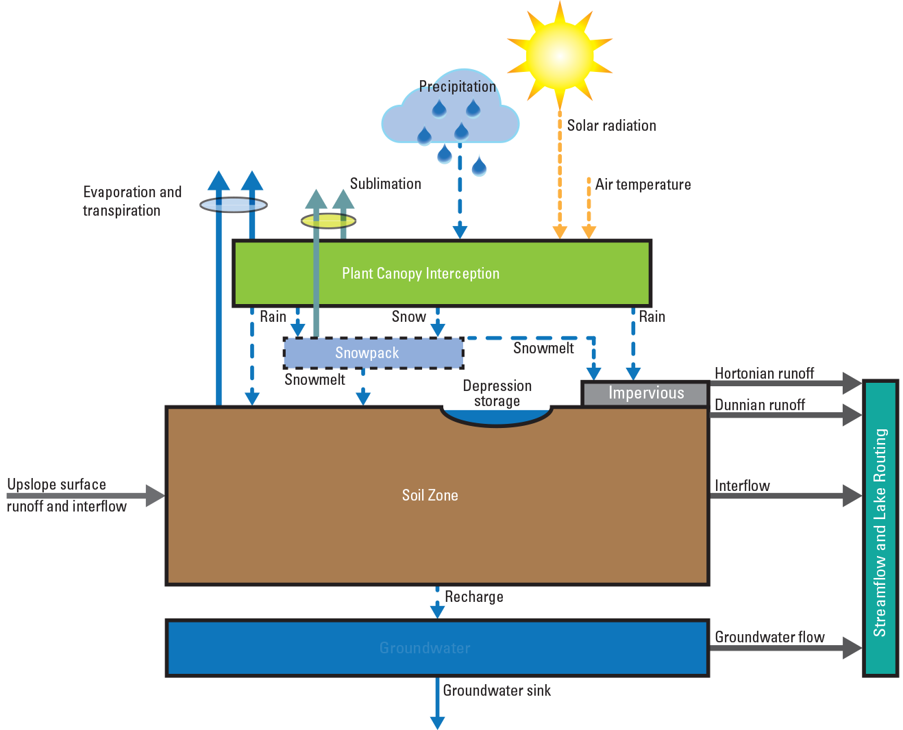
Precipitation-Runoff Modeling System conceptualization (adapted from Regan and LaFontaine, 2017).
Spatial Discretization of Modeling Units
The distributed-parameter capabilities of the PRMS are provided by partitioning the study area into HRUs for which a water balance and an energy balance are computed. The PRMS uses daily climate values of precipitation accumulation and maximum and minimum air temperature distributed to each HRU to compute solar radiation, potential evapotranspiration, actual evapotranspiration, sublimation, snowmelt, streamflow, infiltration, and groundwater recharge. This study used the NHM-PRMS application of the USGS NHM infrastructure (Regan and others, 2018, 2019) that is based on the CONUS region of the GeoSpatial Fabric developed by Viger and Bock (2014). A total of 109,951 HRUs, with a mean area of 75 km2, are included in the NHM-PRMS hydrologic model (fig. 2).
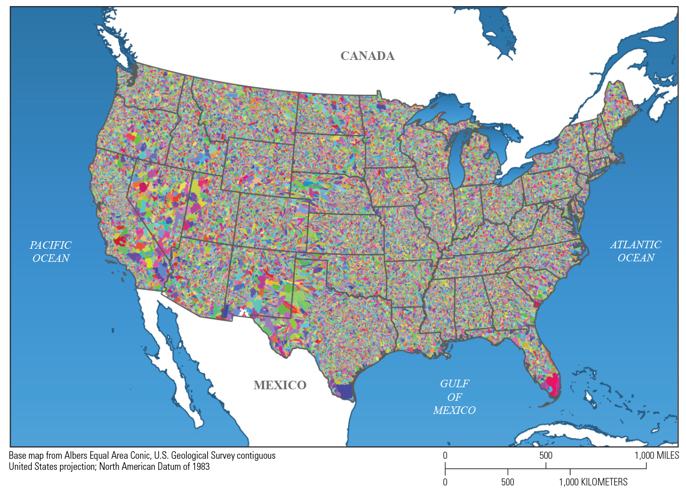
Map showing hydrologic response units used in the National Hydrologic Model infrastructure application of the Precipitation-Runoff Modeling System for the conterminous United States. Colors show spatial discretization only for the 109,951 hydrologic response units.
Parameterization of Model Values
The initial set of NHM-PRMS parameter values used for this application were obtained from the USGS NHM Parameter Database (Driscoll and others, 2017). These parameter values were either universal default values (undistributed) or were modified (distributed by HRU) based on (1) long-established defaults on the basis of hydrologic and geographic information gained across 35 years of PRMS operation; (2) estimation methods described by Viger and Leavesley (2007) for characterizing topography, land cover, soils, geology, and hydrography; (3) direct solution of PRMS algorithms for unknown variables (such as solar radiation and potential evapotranspiration parameters); (4) long-term simulation averaged values (such as initialization parameters for water flux and storage); or (5) estimation methods using other hydrologic simulation results (see Regan and others, 2018, 2019). Many of the parameters in the NHM-PRMS application vary spatially based on the surface and subsurface characteristics of the model domain. The PRMS parameters describe processes such as solar radiation, potential evapotranspiration, canopy interception, snow dynamics, surface runoff, soil-zone dynamics, groundwater flow, and streamflow generation. In the NHM-PRMS, the soil-zone and groundwater reservoirs have the same spatial delineations (size and shape) as the HRUs. The NHM-PRMS parameters with universal default values are undistributed because no methodology was determined to estimate the spatial variability. Table 1 lists the PRMS parameters chosen for calibration and indicates whether the initial values were distributed.
Table 1.
Selected parameters, parameter value ranges, and calibration methods for the three-step calibration procedure: “byHRU” (by hydrologic response unit) represents part 1, “byHW” (by headwater) represents part 2, and “byHWobs” (by headwater with observations) represents part 3. See Markstrom and others (2015) for additional parameter information. The percent method uses the model parameter value to set the extent of the allowable calibration values. The range method uses specified values to set the extent of the allowable calibration values.[*, parameter is calibrated if there is a history of snow accumulation in the watershed of interest; >, greater than]
Climate Forcing Data
The PRMS requires climate forcing inputs of daily maximum and minimum air temperature and daily precipitation time-series data. Climate forcing inputs from the Daymet version 3 climate dataset (Thornton and others, 2017) were used for hydrologic simulations. The Daymet version 3 climate forcings were developed by Thornton and others (2017) for a 1-km grid for North America and are based on measured, at-site air-temperature and precipitation data for 1980–2019. Various preprocessed, gridded datasets are available from the USGS Geo Data Portal (Blodgett and others, 2011), including Daymet version 3. The Geo Data Portal was used in conjunction with a geographic information system shapefile of the model HRUs to transfer the gridded maximum and minimum air temperature and precipitation values to the model HRUs for each day of the study period. The Geo Data Portal used a weighted-areal-averaging algorithm to transfer the values.
NHM-PRMS Calibration
A three-part procedure was used to calibrate the NHM-PRMS for the CONUS. Initial development of the calibration procedure was presented in LaFontaine and others (2019) for an application of the NHM-PRMS in the southeastern United States. The calibration procedure considers water balance volume for each hydrologic response unit (byHRU), streamflow timing in headwater watersheds with drainage areas less than 3,000 km2 (byHW), and calibration to observed streamflow in those headwater watersheds that had streamgages within their domain (byHWobs). Figure 3 outlines the three-part calibration procedure presented in this report as applied to the NHM-PRMS. Figure 4 shows where each level of calibration (byHRU, byHW, and byHWobs) occurs throughout the CONUS.
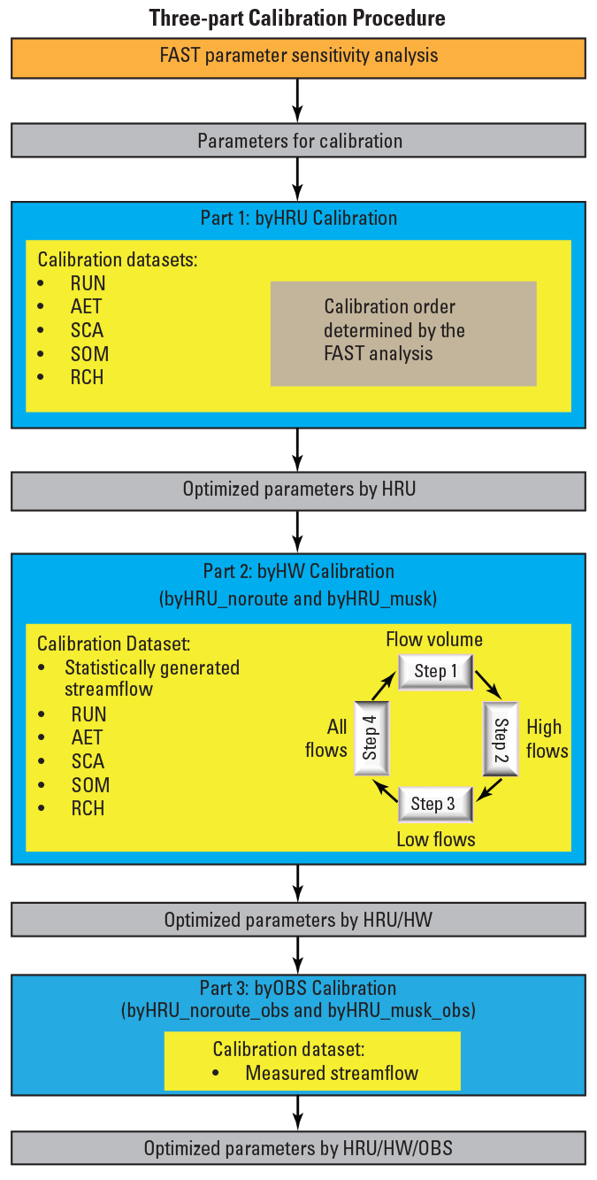
Schematic showing the three-part calibration as applied to the U.S. Geological Survey National Hydrologic Model infrastructure application of the Precipitation-Runoff Modeling System. Abbreviations: FAST, Fourier Amplitude Sensitivity Test; HRU, hydrologic response unit; HW, headwater; OBS, observed.
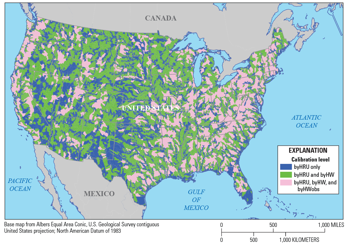
Map showing the level of calibration for model hydrologic response units (HRUs): blue indicates byHRU calibration only; green indicates byHRU and byHW calibration only; and pink indicates byHRU, byHW, and byHWobs calibration. Abbreviations: HW, headwater; OBS, observed.
The following sections describe the three-part calibration procedure. The reader is referred to appendix 1 for details on the necessary file content and directory structure for the three-part calibration procedure using the USGS NHM infrastructure application of the NHM-PRMS (Regan and others, 2018, 2019).
Part 1: Calibration of Hydrologic Response Unit (byHRU calibration)
To calibrate each HRU, the byHRU calibration optimized the water-balance volume between NHM-PRMS simulations and five selected non-streamflow datasets, hereafter referred to as “baseline data products.” The baseline data products were derived, with error bounds, from multiple sources for each of the 109,951 HRUs in the NHM infrastructure (fig. 2) at daily, monthly, and annual time steps. Results from a Fourier Amplitude Sensitivity Test (FAST; Cukier and others, 1973; Schaibly and Shuler, 1973; Cukier and others, 1975; Saltelli and others, 2006; Markstrom and others, 2016) were used to identify the relative sensitivity of each calibration dataset to the parameters chosen for calibration (table 1). An automated calibration procedure that incorporated the Shuffled Complex Evolution algorithm (Duan and others, 1992, 1993, 1994) was used to identify the optimal model parameter sets for each HRU.
Baseline Calibration Datasets
For each HRU in the NHM-PRMS, calibration baseline datasets were derived, with error bounds, for runoff, actual evapotranspiration, recharge, soil moisture, and snow-covered area. Monthly values of runoff by HRU were derived from the NHM application of the MWBM (NHM-MWBM) developed by Bock and others (2016) (also see table 2), which used a parameter-regionalization procedure that transferred parameter values from gaged to ungaged areas, producing simulated runoff for all HRUs in the NHM infrastructure. The NHM-MWBM output for the CONUS is available on the USGS Monthly Water Balance Model Futures Portal (Bock and others, 2017). Bock and others (2018) used a stochastic, post-processing framework developed by Bourgin and others (2015) and Farmer and Vogel (2016) to quantify uncertainty in simulated monthly runoff produced by the NHM-MWBM. This uncertainty was treated as an error bound for the use of the NHM-MWBM outputs in the runoff baseline dataset used in this study.
Table 2.
List of baseline datasets used in the calibration procedure, the method used to derive a calibration range for each of the five water budget components, the PRMS output variable that was compared to that calibration range for each water budget component, the time step used for comparison, and the period of record compared. For actual evapotranspiration, recharge, and soil moisture, multiple datasets were combined into one calibration dataset per water budget component. For snow-covered area, a calibration range was derived from that dataset’s confidence interval information. For runoff, a confidence interval was previously developed by Bock and others (2018).[PRMS, Precipitation-Runoff Modeling System; SSEBop, Simplified Surface Energy Balance; MOD16, MODIS Global Evapotranspiration Project; Do. or do., ditto; WaterGAP, Water—Global Assessment and Prognosis model; MERRA, Modern-Era Retrospective analysis for Research and Applications; NCEP, National Centers for Environmental Prediction; NCAR, National Center for Atmospheric Research; NLDAS, North American Land Data Assimilation System; CMG, Climate Modeling Grid]
Monthly ranges of actual evapotranspiration by HRU were derived using (1) the NHM-MWBM (Bock and others, 2017), (2) the MOD16 global evapotranspiration product (https://modis.gsfc.nasa.gov/data/dataprod/mod16.php), and (3) the Simplified Surface Energy Balance (SSEBop) model (Senay and others, 2013; table 2). Based on these three data products, a range of actual evapotranspiration was calculated, and the range defines the error bound for each HRU on a monthly and mean-monthly time step for the period 2000–2010.
Annual ranges of recharge by HRU were derived using (1) empirical regression estimates of total recharge (Reitz and others, 2017) and (2) recharge from the WaterGAP 2.2a prognosis model (Döll and others, 2014; table 2). An initial comparison of recharge from these two products and from the NHM-PRMS showed substantial differences in recharge magnitude, most likely due to (1) conceptual differences in representing recharge and (2) associated hydrologic processes in creating each dataset. Therefore, the annual recharge values from the two datasets were normalized for the range from 0 to 1 over the period 2000–2009, and the optimization scheme targeted the similarity in the relative change from year to year. Based on these two data products, a range of normalized recharge was calculated on an annual time step and treated as an error bound for each HRU. The normalized recharge rate was also used to calibrate the NHM-PRMS for the available recharge period of record.
Soil moisture is an important variable in PRMS, representing antecedent moisture conditions in a watershed, and has been used to help calibrate hydrologic models (Thorstensen and others, 2016; Li and others, 2018). Including soil moisture in hydrologic model calibration has also been shown to help address equifinality issues (Li and others, 2018). However, ground-based soil-moisture datasets have limited spatial coverage (Romano, 2014). Remote-sensing techniques that provide spatially distributed values of soil moisture would be valuable (Li and others, 2016) and could be considered in future studies when a longer time period is available. An example collection platform is the Soil Moisture Active Passive (https://smap.jpl.nasa.gov/) satellite-based data products. Monthly and annual ranges of soil moisture were derived for each HRU using soil-moisture values from the following model applications: (1) the MERRA-Land reanalysis (https://gmao.gsfc.nasa.gov/reanalysis/MERRA-Land/data), (2) the NCEP-NCAR reanalysis (https://psl.noaa.gov/data/gridded/data.ncep.reanalysis.html), (3) the NLDAS-MOSAIC model (https://ldas.gsfc.nasa.gov/nldas/nldas-2-model-data), and (4) the NLDAS-NOAH model (https://earthdata.nasa.gov/; table 2).
The soil moisture from these datasets was normalized in the same way as recharge with values ranging from 0 to 1 for annual or monthly values over the period 1982–2010. The soil moisture from the upper soil layer was used from each model and compared with the PRMS variable soil_rechr. The PRMS variable soil_rechr represents the storage for the upper part of the capillary reservoir and is thought to be most comparable to the upper soil layer from the four datasets listed in table 2 for soil moisture. It was not expected that the soil-moisture magnitudes from these four products and soil_rechr from PRMS would equate. Rather, the optimization scheme targeted the similarity in the relative change. Based on the four soil-moisture data products (table 2), a range of soil moisture was calculated and treated as an error bound for each HRU on a monthly and annual basis and was then used as a target for the PRMS calibration.
Daily values of snow-covered area by HRU were derived from the Moderate Resolution Imaging Spectrometer (MODIS)/Terra Snow Cover Daily L3 Global 0.05Deg CMG dataset (MOD10C1; Hall and Riggs, 2016; table 2). The daily snow-covered area values have an associated confidence interval, where a confidence interval equal to 100 percent indicates clear sky conditions with the highest level of confidence. The monthly MODIS snow-covered area (SCA) product does not use snow-covered area values unless the confidence interval is greater than 70 percent. For this study, daily values of snow-covered area were used if the confidence interval was greater than 70 percent. The upper and lower range for the daily snow-covered area value for each HRU was calculated and treated as an error bound based on the daily snow-covered area value and the associated confidence interval for the period 2000–2010 and was used as a target for the NHM-PRMS calibration.
Figure 5A shows the mean and figure 5B shows the mean of the range for each baseline dataset for all HRUs. The datasets and associated time-periods described in table 2 were used to derive each baseline mean and range dataset. The runoff mean was calculated as the mean of the monthly NHM-MWBM values. The actual evapotranspiration mean was calculated as the monthly mean derived from the mean of three source values (see table 2). The mean snow-covered area was calculated as the daily mean for days with snow present and a confidence interval greater than 70 percent. The soil moisture and recharge means were calculated as the normalized monthly and annual mean values from the respective source values (table 2). Figure 5C shows the mean divided by the mean of the range (mean/range) for each HRU and baseline dataset. Values above 1.0 indicate that the mean tends to be greater than the range while values below 1.0 indicate that the mean tends to be less than the range. In figure 5C, the dark-green areas represent locations that have a relatively low range with respect to the mean. This could indicate greater confidence in the baseline, but it also indicates that the calibration procedure will have a smaller range to fit. Dark-red areas in figure 5C represent a relatively high range around the mean, which possibly indicates low confidence in the baseline but also indicates a much easier fit in the calibration procedure.
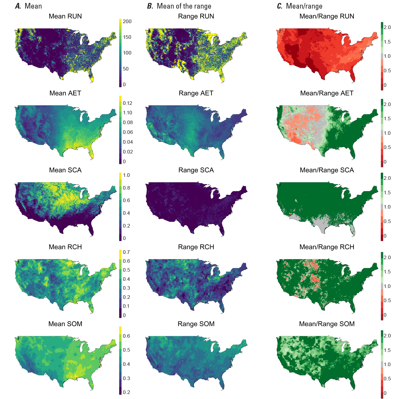
Maps showing baseline dataset A, mean; B, mean of range; and C, mean/mean of the range, for (1) runoff (RUN), in cubic feet per second; (2) actual evapotranspiration (AET), in inches per day; (3) snow-covered area (SCA), expressed as fraction covered, where 1 = fully covered; (4) recharge (RCH), in inches per day; and (5) soil moisture (SOM), as depth in inches. For RCH and SOM, units of depth are normalized to dataset maximums and minimums. Vertical scales between columns A and B apply to both A and B.
PRMS Sensitivity Test
Markstrom and others (2016) used the FAST procedure (Cukier and others, 1973; Schaibly and Shuler, 1973; Cukier and others, 1975; Saltelli and others, 2006) to identify dominant hydrologic processes (such as baseflow, evapotranspiration, runoff, infiltration, snowmelt, soil moisture, surface runoff, and interflow) based on a CONUS-wide sensitivity analysis of PRMS parameters from the NHM infrastructure. This same procedure was used to identify the relative sensitivity of the PRMS outputs of runoff, actual evapotranspiration, recharge, soil moisture, and snow-covered area to the PRMS parameters chosen for calibration (table 1). The FAST procedure is a variance-based global sensitivity algorithm that estimates the contribution to model output variance explained by each parameter (Cukier and others, 1973, 1975; Saltelli and others, 2006). The FAST procedure transforms the multi-dimensional parameter space of a model into a single dimension of mutually independent sine waves with varying frequencies for each parameter. The FAST method uses the parameter ranges to define each wave’s amplitude (Cukier and others, 1973, 1975; Reusser and others, 2011). This methodology creates an ensemble of parameter sets, each of which is unique and non-correlated with the other parameter sets. The NHM-PRMS model was executed for all parameter sets, and, for every HRU, the relative influence of each baseline dataset was determined. Figure 6 shows the relative influence (or weights) for each of the baseline datasets (fig. 6A through E) and the dominant PRMS variable (fig. 6F).
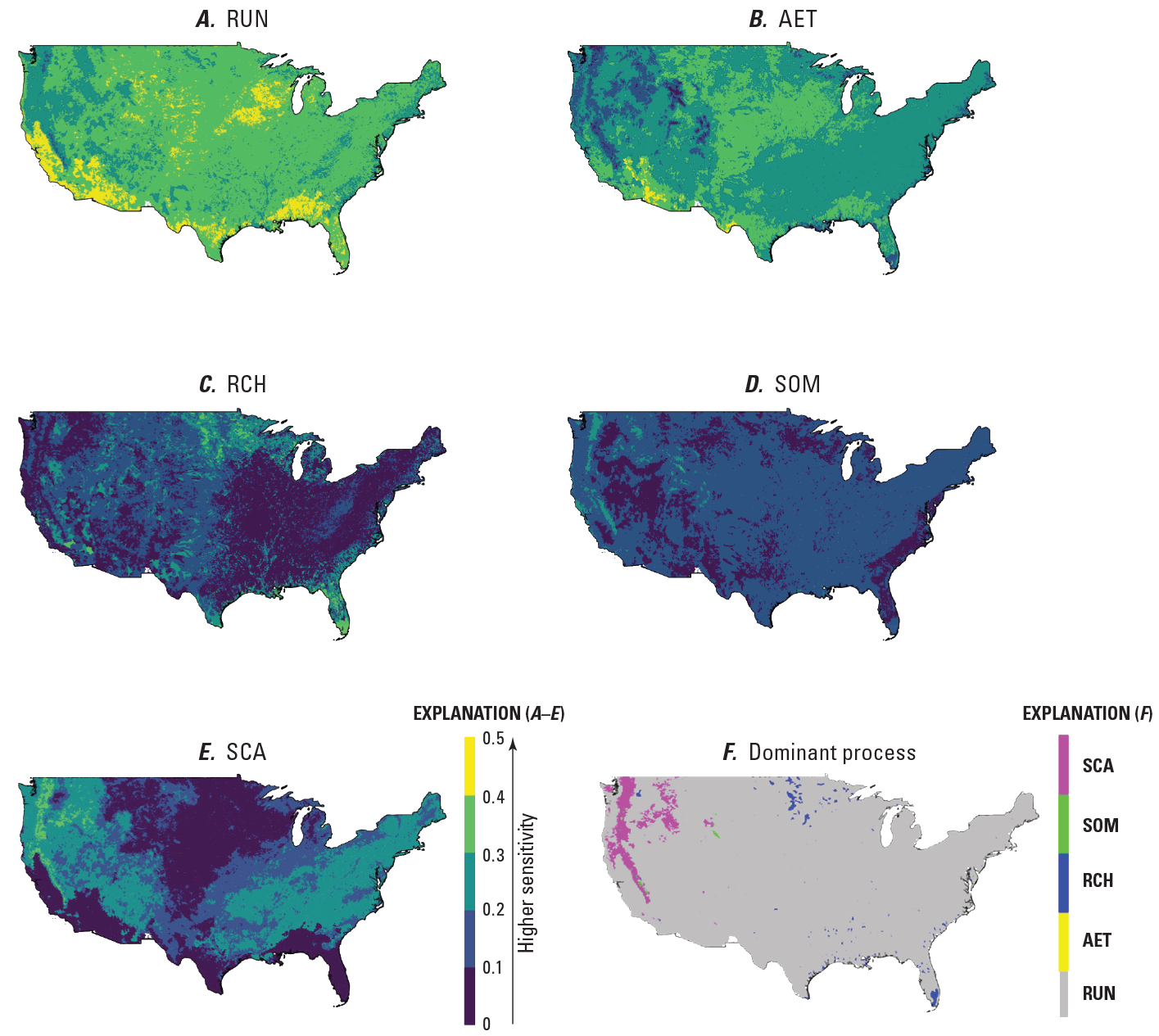
Maps showing Precipitation-Runoff Modeling System (PRMS) output variable weights from Fourier Amplitude Sensitivity Test (FAST) analysis for A, runoff (RUN); B, actual evapotranspiration (AET); C, recharge (RCH); D, soil moisture (SOM); E, snow-covered area (SCA); and F, dominant PRMS variable based on FAST analysis.
Calibration Procedure
The byHRU calibration uses a multiple-objective, stepwise, automated calibration procedure using the Shuffled Complex Evolution (SCE) global optimization algorithm (Duan and others, 1992, 1993, 1994). The SCE global optimization algorithm addresses the difficulties in optimization when there are several regions of attraction and multiple local optima in the parameter space. The SCE algorithm avoids the problem of being trapped in local optima by using a population-evolution-based global search technique which searches for the optimal solutions from a population of possible solution points, rather than a single point. For more information on how the SCE algorithm is configured for calibration, the reader is referred to Hay and Umemoto (2007).
The objective function for each step in the byHRU calibration targeted the minimization of the normalized root mean square error (NRMSE) computed as shown in equation 1.
wheren
is the time step;
nstep
is the total number of time steps;
MSDn
is the values from the baseline dataset;
SIMn
is the PRMS-simulated values; and
MN
is the mean of all baseline values for the objective function time period.
For each HRU, the order of the five steps in the stepwise procedure was determined based on the NHM-PRMS variable weights (from high to low sensitivity) from the FAST analysis for that HRU (fig. 6). The first step calibrated all the parameters using the parameter ranges listed in table 1. The parameter range for the first calibration step was based on either the acceptable range presented in table 1 or by adding +/− 20 percent of the range to the initial value. If the parameter had a constant value for all HRUs (in other words, if the parameter was not spatially distributed based on some parameterization dataset), then the range method was used. If the parameter was spatially distributed (as described by Regan and others, 2018), then the percent method was used. For the remaining calibration steps, all parameters were calibrated, but the parameter range was refined based on optimized parameter values from the top 25 percent of the objective functions (objective function is minimized) from the previous step. The final (sixth) step calculated the NRMSE using all baseline datasets, weighting the objective function summation based on the NHM-PRMS variable weights from the FAST analysis. If there was no sensitivity of parameters to the baseline dataset (such as SCA in basins with no snow), then that calibration step was skipped.
Figure 7 shows the sequencing of the soil_rechr_max_frac parameter calibration range refinements for an example HRU. The baseline datasets for this HRU were calibrated in the order shown in figure 7A through F based on the FAST results described under “PRMS Sensitivity Test.” The soil_rechr_max_frac parameter represents a soil-zone storage threshold that defines the maximum storage for the soil recharge zone (the upper part of a capillary reservoir where losses occur as both evaporation and transpiration) as a fraction of maximum available water-holding capacity, which is represented by the parameter soil_moist_max (Regan and LaFontaine, 2017). For each HRU, the initial values for the soil_rechr_max_frac parameter were calculated using a multiple-linear regression equation that included geology, drainage density, aquifer type, vegetation type, and base-flow-index information (Viger, 2014; Regan and others, 2018). The parameter range for step 1 in the calibration procedure (y-axis in figure 7A) was calculated using the initial value +/− 0.20 of the range (maximum minus minimum allowable parameter value in table 1).
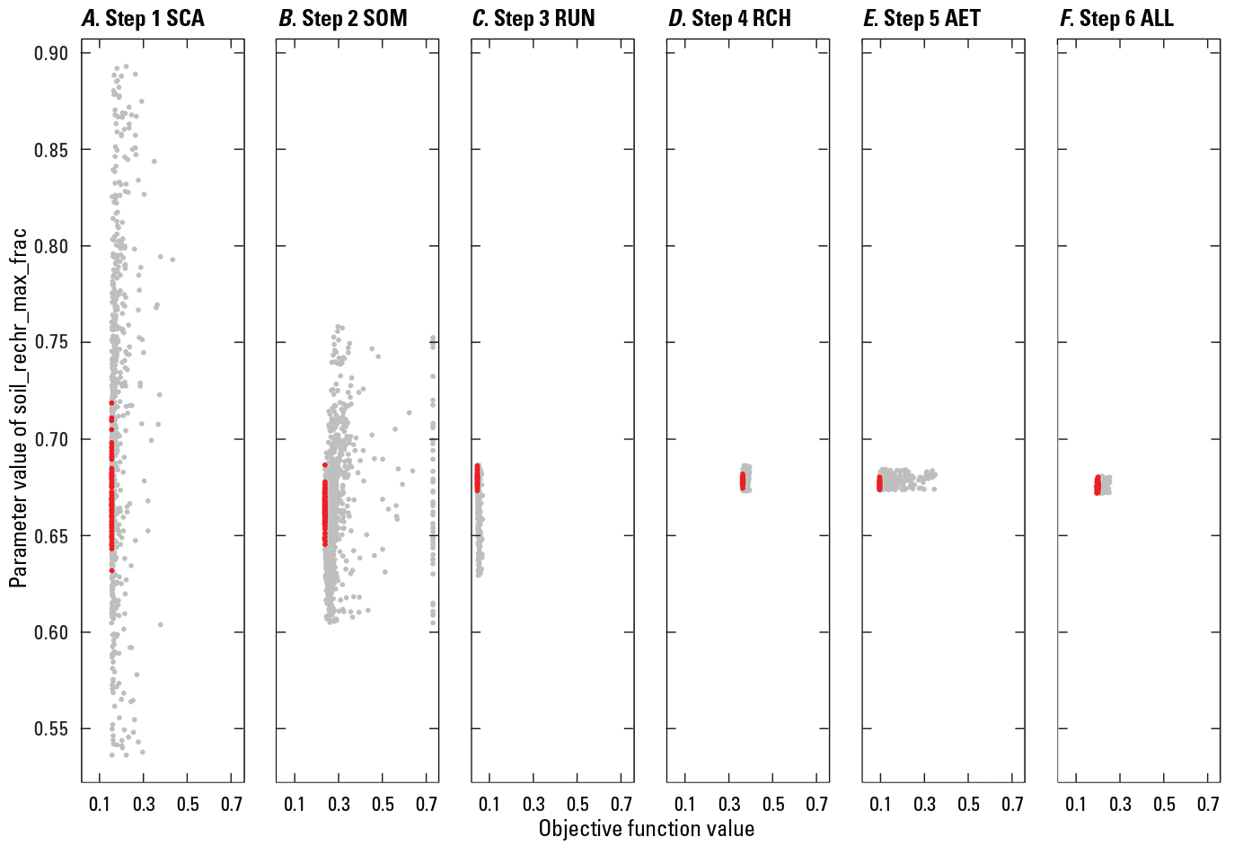
Graphs showing an example of the refinement of the soil_rechr_max_frac parameter range as the calibration proceeds through the six steps: A, step 1 snow-covered area (SCA); B, step 2 soil moisture (SOM); C, step 3 runoff (RUN); D, step 4 recharge (RCH); E, step 5 actual evapotranspiration (AET); and F, step 6 all baseline datasets (ALL). The y-axis of each panel represents the parameter values tested for soil_rechr_max_frac for a particular calibration step. The x-axis of each panel represents the objective function value for each calibration run in each step. In each panel, dots toward the left have lower (“better”) objective function values and dots toward the right have higher (“worse”) objective function values. Red dots indicate the parameter values that had the lowest 25 percent of objective function values for inclusion in the next calibration step. Gray dots indicate the parameter values that were tested but not selected for inclusion in the next calibration step. The six steps were ordered based on sensitivity analysis results from Markstrom and others (2016).
Part 2: Calibration for Headwater Watersheds (byHW Calibration)
The byHRU calibration produced spatially distributed parameter values for every HRU in the NHM-PRMS (fig. 2). The byHRU calibrated parameter values are used as initial values for the byHW calibration. In the CONUS, 7,265 watersheds were identified as headwater watersheds with drainage areas less than 3,000 km2 (1,158 mi2); this area represents an upper limit for an approximate instream travel time of one day. The drainage outlet of each headwater watershed was identified, and the Bandit software tool (Regan and others, 2018) was used to extract complete sets of input files that contain the model parameters and climate forcings required for an NHM-PRMS model simulation. The green and pink areas in figure 4 show the extent of the headwater watersheds for the CONUS. Each extracted headwater watershed model was calibrated separately, and calibrated parameter values were returned to the NHM-PRMS.
Statistical Time Series of Streamflow
For this study, the byHW calibrations use statistically based daily streamflow simulations developed using ordinary kriging (Farmer, 2016) along with the baseline data products (described in table 2) as calibration targets for each headwater watershed. The statistically based daily time-step streamflow simulations were developed for use as calibration datasets for the 7,265 headwater watersheds in the CONUS. Ordinary kriging is a geostatistical tool that uses the distance between two points on the landscape (for example, streamgage locations) to predict the semi-variance of a dependent variable. LaFontaine and others (2019) documented the procedure used to generate the statistical time series. The maximum, minimum, and median simulated daily streamflows generated from the ordinary kriging analysis were used for NHM-PRMS byHW model calibration. The environmental flow components (EFC) algorithm developed by The Nature Conservancy (2009) was used to categorize the daily statistical time series of streamflow into high- and low-flow values. For this study, high flows consisted of streamflows categorized by the EFC algorithm as large floods, small floods, or high-flow pulses. Low flows consisted of streamflows categorized by the EFC algorithm as low or extreme low flows.
Farmer and others (2019) used statistical simulations in place of measured streamflow to calibrate hydrologic models across the CONUS and concluded that the statistically generated streamflow time series provided valuable streamflow timing information and could be combined with non-streamflow datasets to improve hydrologic-process representation at ungaged locations. For this study, the byHW calibration uses statistically based daily streamflow simulations developed using ordinary kriging (Farmer, 2016) along with the five non-streamflow data products described in table 2 as calibration targets for each headwater watershed. The byHW calibration is considered a streamflow timing calibration and, as such, two PRMS routing methods are tested and documented below and in appendix 2.
Streamflow Routing
This study tests two PRMS routing methods, which are referred to as byHRU_noroute and byHRU_musk calibrations. The byHRU_noroute calibration uses the PRMS module strmflow_in_out. Streamflow through segments is routed as inflow equals outflow to maintain continuity, but this routing does not delay or attenuate streamflow (Markstrom and others, 2015). The byHRU_musk uses the PRMS module: muskingum_mann: the Muskingum routing method for attenuation of streamflow (Linsley and others, 1982; Mastin and Vaccaro, 2002; Markstrom, 2012; Markstrom and others 2015). Appendix 2 describes the input parameters used in the Muskingum-based routing module, muskingum_mann.
Calibration Procedure
The byHW calibration procedure (the second step in fig. 3) adjusts parameters using a four-step multiple-objective procedure (Hay and others, 2006a; Hay and Umemoto, 2007) using the SCE global search algorithm (Duan and others, 1992, 1993, 1994). The match between simulated and statistically based streamflows was optimized by comparing: (step 1) streamflow volume, (step 2) timing and magnitude of EFC-categorized high-flow days, (step 3) timing and magnitude of EFC-categorized low-flow days, and (step 4) timing and magnitude of all days. Table 1 lists the parameters chosen for the byHW calibration. All selected parameters were calibrated in each of the four steps, but only the parameter range identified by the FAST analysis and noted in the last column in table 1 was used for calibration.
The NHM-PRMS parameters were calibrated by adjusting the mean parameter values for HRUs within each headwater watershed. Each execution of the SCE algorithm produced a new mean for the parameter values. The new mean parameter values were redistributed to headwater HRUs based on the previous distribution of the HRU parameter values. For each calibration step, the parameters identified for that step were calibrated using the minimum and maximum allowable parameter values listed in table 1. Parameters not associated with a given step were still adjusted but were only allowed to vary by +/−10 percent of their initial value. For example, the fastcoef_lin parameter is listed in table 1 as being calibrated in step 3. The range for the fastcoef_lin parameter in the first step would therefore be calculated as the initial value (based on the byHRU calibration) +/− 0.10 × (0.6 − 0.01). If there was no sensitivity of parameters to snow processes, then the snow parameters were not calibrated (noted by an asterisk in table 1).
The objective function for each step in the byHW calibration used the NRMSE metric (eq. 1). The objective function for each calibration step was calculated using equation 2. The extracted NHM-PRMS headwater watershed models were run for the period from October 1, 1980, to September 30, 2010, but only odd calendar years were used for calibration; this allowed for the even calendar years to be used for evaluation. Table 3 describes the objective functions that used the statistically generated streamflow and associated weights for each calibration step. The objective function weights were based on trial-and-error and expert knowledge and could be the focus of future research on improving calibration methods. The objective functions were computed as weighted sums of NRMSE and were calculated on monthly, mean monthly, and daily time steps with subsets of high- and low-flow days using daily time steps (table 3). The NRMSE was calculated two ways: computing error if (1) the simulated value fell inside or outside of the target range or (2) using the median value of the range of values in the calibration dataset for each time step. For the first option, if the simulated value for a time step was between the upper and lower bounds of the calibration dataset, the difference between simulated and observed was assumed to be zero. For the second option, a single value was computed for each time step in the calibration dataset. The computed value was then compared to the simulated values. The OFstep was computed as follows:
whereOFstep
is the aggregated objective function value;
OF1
is the objective function for monthly streamflow range of the ordinary kriging-based streamflow time series;
OF2
is the objective function for mean monthly streamflow range of the ordinary kriging-based streamflow time series;
OF3
is the objective function for monthly streamflow median of the ordinary kriging-based streamflow time series;
OF4
is the objective function for mean monthly streamflow median of the ordinary kriging-based streamflow time series;
OF5
is the objective function for daily streamflow using the range of the ordinary kriging-based streamflow time series;
OF6
is the objective function for daily streamflow high-flow days using the median of the ordinary kriging-based streamflow time series;
OF7
is the objective function for daily streamflow low-flow days using the median of the ordinary kriging-based streamflow time series; and
w
is the weight for each objective function;
OFbase
sum of the NRMSE using all five baseline datasets, divided by 5 (weight in table 3).
Part 3: Calibration for Headwater Watersheds with Measured Streamflow (byHWobs)
Part 3 of the calibration procedure, the byHWobs calibration, refined the final parameter values from Part 1 and Part 2 (see fig. 3) using available measured streamflow in the headwater watersheds. Two methods were tested: (1) byHRU_musk_obs, which used the final parameters from the byHRU_musk calibration and (2) byHRU_noroute_obs, which used the final parameters from the byHRU_noroute calibration.
Measured Streamflow
The NHM-PRMS includes 8,274 USGS streamgages in the Geospatial Attributes of Gages for Evaluating Streamflow (GAGES-II) dataset (Falcone, 2011); 2,411 of these streamgages fall within 1,417 of the delineated headwater watersheds in this study (pink areas in fig. 4). The poi_gage_id and poi_gage_segment parameters in the NHM-PRMS parameter file respectively indicate the USGS streamgage station number and the segment index for each streamgage in the NHM-PRMS (Regan and others, 2018). The PRMS-simulated streamflow at each of the poi_gage_segment locations is compared with the measured streamflow in the calibration procedure.
Calibration Procedure
The byHWobs calibration (the first step in fig. 3) started with the final byHW calibration parameter values for the 1,417 headwater watersheds that contained measured streamflow (pink areas in fig. 4). Within those headwater watersheds, there are 2,163 streamgages with streamflow appropriate for model calibration (some headwater watersheds contained more than one streamgage). A one-step, one-round procedure was used to adjust the final parameter values from the byHW calibration based on the available measured streamflow in each headwater watershed. All parameters in table 1, excluding snow parameters when not applicable, were calibrated using ranges calculated as +/− 20 percent of the initial value.
For headwater watersheds with observed streamflow, three weighting factors for each streamgage were calculated in the objective function, as follows: (1) weight based on the size of the watershed area for a given streamgage compared to the total area of the headwater watershed of interest (Wsize), (2) drainage area correction between simulated and published values (Wdac), and (3) correction based on the length of observed streamflow period of record (Wpor). The Wsize gives larger streamgage drainage areas more weight in the objective function calculation, as each streamgage is weighted based on the percent coverage of the headwater watershed (total drainage area of streamgage divided by the drainage area of headwater watershed). The Wdac is a correction factor that was applied to the observed streamflow if the contributing area of the streamgage based on the GeoSpatial Fabric was not the same as the reported National Water Information System (NWIS) contributing area. If the NWIS drainage area (NWISda) was larger than the Geospatial Fabric for National Hydrologic Modeling (GF; Viger and Bock, 2014) drainage area (GFda), then Wdac = GFda ∕ NWISda. If the NWISda was smaller than the GFda, then Wdac = NWISda ∕ GFda. If Wdac was less than 0.9 or greater than 1.1, then that streamgage was not used in the calibration. The Wpor was used to weight objective functions relative to the number of observations (so that longer records get more weight) within a given headwater watershed. Each streamgage is weighted based on the percent coverage of the calibration period.
A multiple-objective automated calibration procedure was used to identify the optimal set of parameters for each calibration procedure. For each streamgage in a given headwater watershed, the objective function was calculated as follows:
whereOFgage
is the objective function at each streamgage;
Wsize
is the drainage area weighting factor;
Wdac
is the drainage area comparison factor;
Wpor
is the length of observed record factor;
NSE
is the Nash-Sutcliffe Efficiency Index; and
NSElog
is the Nash-Sutcliffe Efficiency Index computed with logarithmic values of simulated and measured streamflow.
The Nash-Sutcliffe Efficiency Index (NSE) metric was calculated using equation 4 as follows:
whereNSE
is the Nash-Sutcliffe Efficiency Index;
nstep
is the total number of time steps;
SIMn
is the simulated streamflow for time step n;
MSDn
is the measured streamflow for time step n; and
MN
is the mean of all measured streamflows for all time steps.
The NSE metric with logarithmic values of streamflow (NSElog) was calculated using equation 5 as follows:
whereNSElog
is the Nash-Sutcliffe Efficiency Index computed with logarithmic values of simulated and measured streamflow;
nstep
is the total number of time steps;
SIMn
is the simulated streamflow for time step n;
MSDn
is the measured streamflow for time step n; and
MN
is the mean of all measured streamflows for all time steps.
The byHWobs calibration period was for odd water years of the period 1981–2010 (such as 1981, 1983, 1985, and so forth). Any NSE or NSElog values that were less than zero were multiplied by 0.1 to lower the contribution to the total objective function. This was incorporated because it was decided that all the streamgage data in a headwater watershed should be used, even if there are anthropogenic influences on the streamflow record. The final objective function sums the OFgage values over all gages in a given headwater watershed.
Results
An automated calibration procedure was used to identify the optimal set of parameters for each part of the calibration procedure (fig. 3), providing spatially distributed parameters for the CONUS. Figure 8 shows examples of the final spatial distribution for four of the calibrated parameters: (A) carea_max, (B) gwflow_coef, (C) rad_trncf, and (D) soil_moist_max resulting from the byHRU, byHRU_musk, byHRU_musk_obs, byHRU_noroute, and byHRU_noroute_obs calibrations, respectively. The relative smoothness of the parameter map in the byHRU calibration becomes more mosaicked as the calibration proceeds due to the incorporation of streamflow data for calibration.
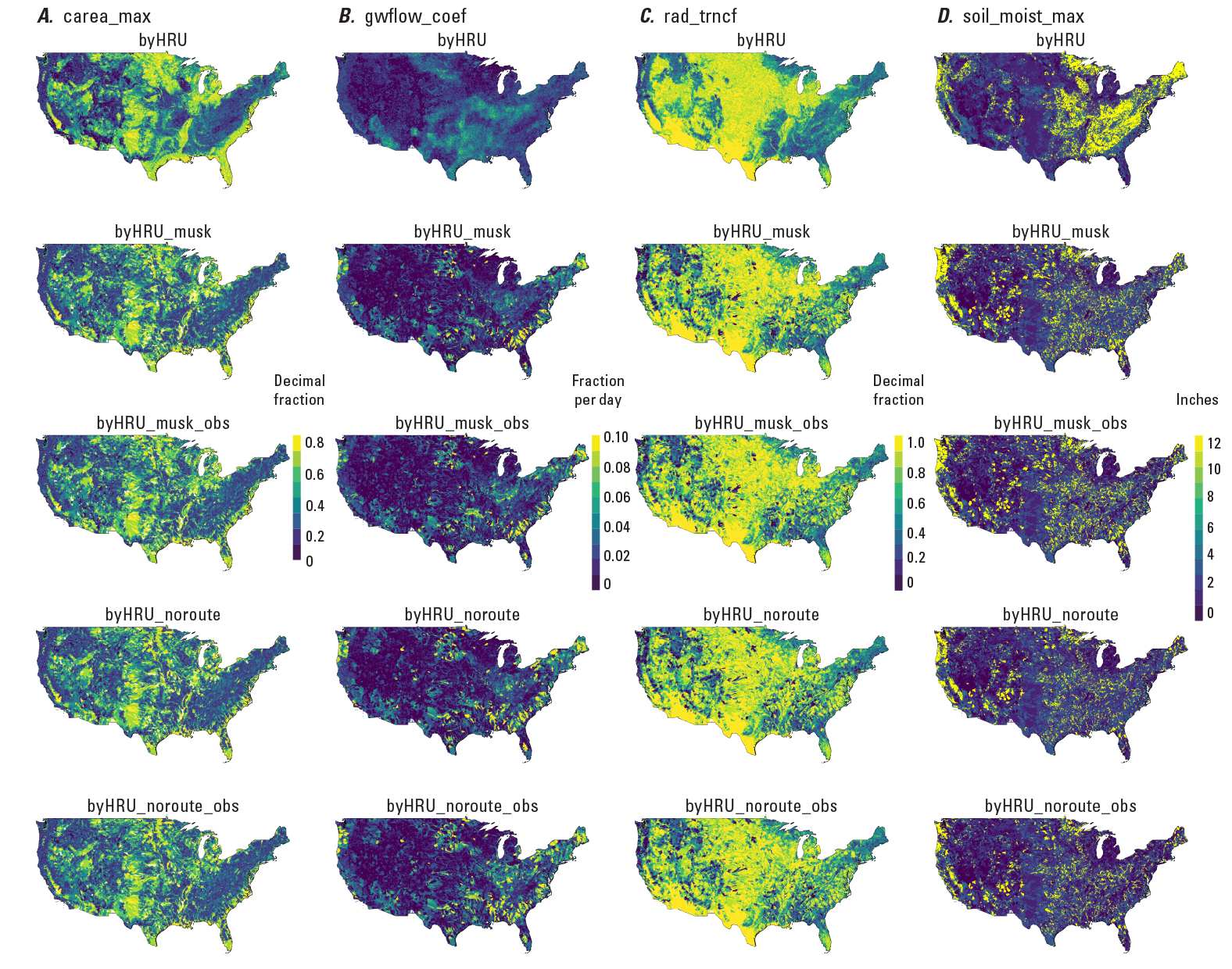
Maps showing calibrated parameter values for: A, carea_max; B, gwflow_coef; C, rad_trncf; and D, soil_moist_max. The rows represent the byHRU, byHRU_musk, byHRU_musk_obs, byHRU_noroute, and byHRU_noroute_obs calibrations. The color scales for each column represent the parameter values for the model HRUs for each calibration version.
Comparisons Between Simulated Values and byHRU Calibration Datasets
The maps in figures 9–13 indicate the percent of time the PRMS-simulated variables that align with the baseline calibration datasets (using the optimal parameters from the byHRU, byHRU_musk, byHRU_musk_obs, byHRU_noroute, and byHRU_noroute_obs calibrations) fell within the range of the observed baseline calibration datasets (see table 2) for runoff, actual evapotranspiration, recharge, soil moisture, and snow-covered area, respectively. Figure 9 shows measured baseline fit for monthly and mean monthly runoff. In general, mean monthly showed a better fit within the range compared with monthly. The byHRU results showed the best fits overall. These results were somewhat constrained as the calibration proceeded, fitting parameters to statistically generated and measured streamflow in the byHW (byHRU_musk and byHRU_noroute) and byHWobs (byHRU_musk_obs and byHRU_noroute_obs) calibrations, respectively. Figure 10 shows measured baseline fit for monthly and mean monthly actual evapotranspiration. In general, the mean monthly time step shows a better fit within the range compared with monthly. The byHRU results showed the best fits overall, but the results were quite similar as the calibration proceeded, fitting parameters to statistically generated and measured streamflow in the byHW (byHRU_musk and byHRU_noroute) and byHWobs (byHRU_musk_obs and byHRU_noroute_obs) calibrations, respectively.
Values of actual evapotranspiration compared well in the central and western United States, with less accuracy in the southeastern United States. Figure 11 shows measured baseline fit for recharge baselines derived from normalized annual values. There was little noticeable change in the baseline fit as the calibration proceeded. Figure 12 shows measured baseline fit for soil moisture baselines derived from normalized annual and monthly values. In general, the annual comparisons had a better fit within the range compared with the monthly comparisons. The byHRU results showed the best fits overall, but the results were quite similar as the calibration proceeded, fitting parameters to statistically generated and measured streamflow in the byHW (byHRU_musk and byHRU_noroute) and byHWobs (byHRU_musk_obs and byHRU_noroute_obs) calibrations, respectively. Figure 13 shows measured baseline fit for daily snow-covered area baselines. There was little noticeable change in the baseline fit as the calibration proceeded. Regions of lower percent within bounds values are associated with locations having the most snow-covered area. Regions of higher percent within bounds values are associated with locations that have generally low to no snow-covered area values.
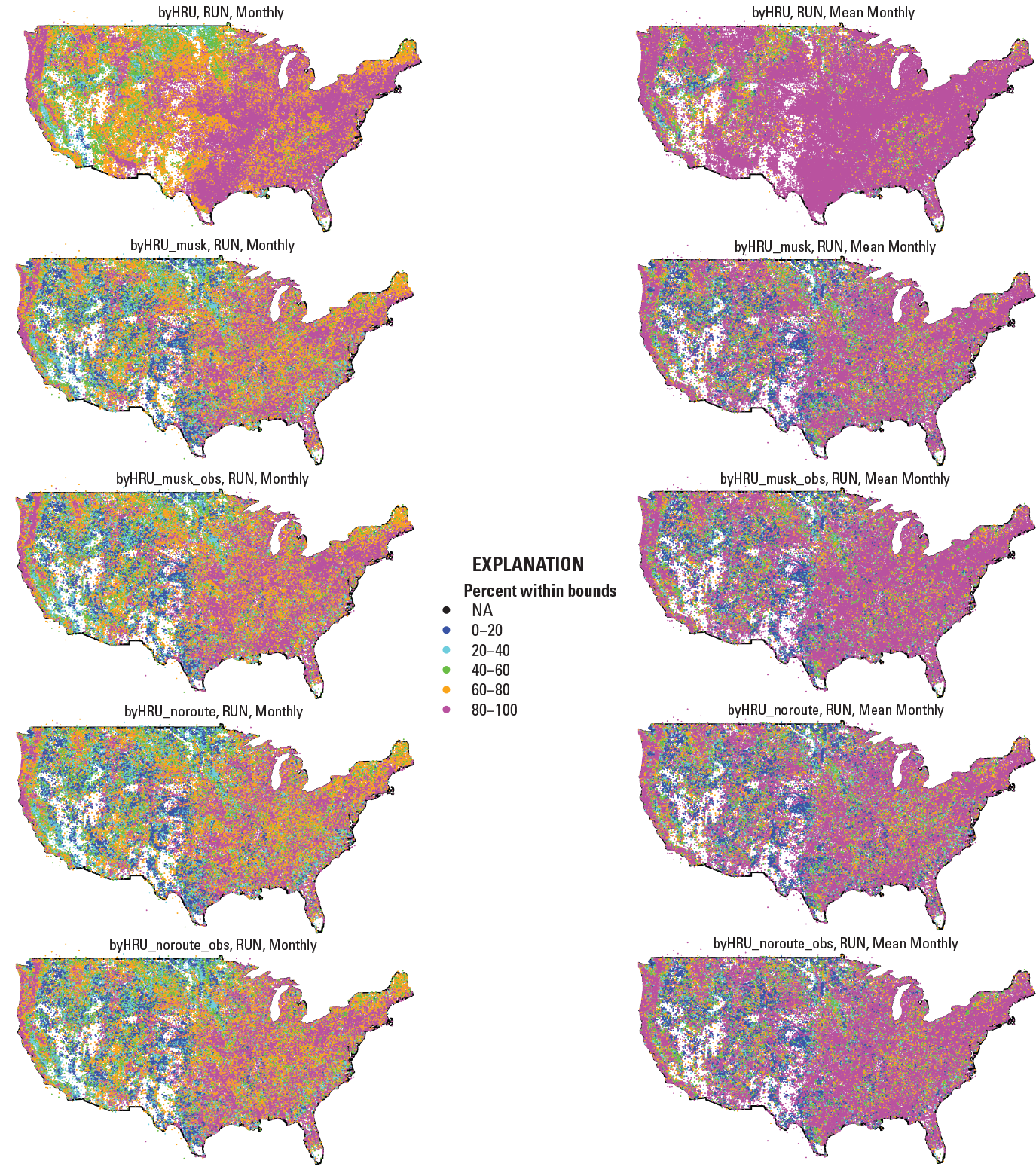
Maps showing percent of the time that simulated runoff (RUN; Precipitation-Runoff Modeling System variable basin_cfs) fell within the range of the measured RUN baseline. The columns represent monthly and mean monthly RUN baselines. The rows represent the byHRU, byHRU_musk, byHRU_musk_obs, byHRU_noroute, and byHRU_noroute_obs calibrations. A value of NA indicates that no comparison was made between simulated and measured values for that hydrologic response unit (HRU).
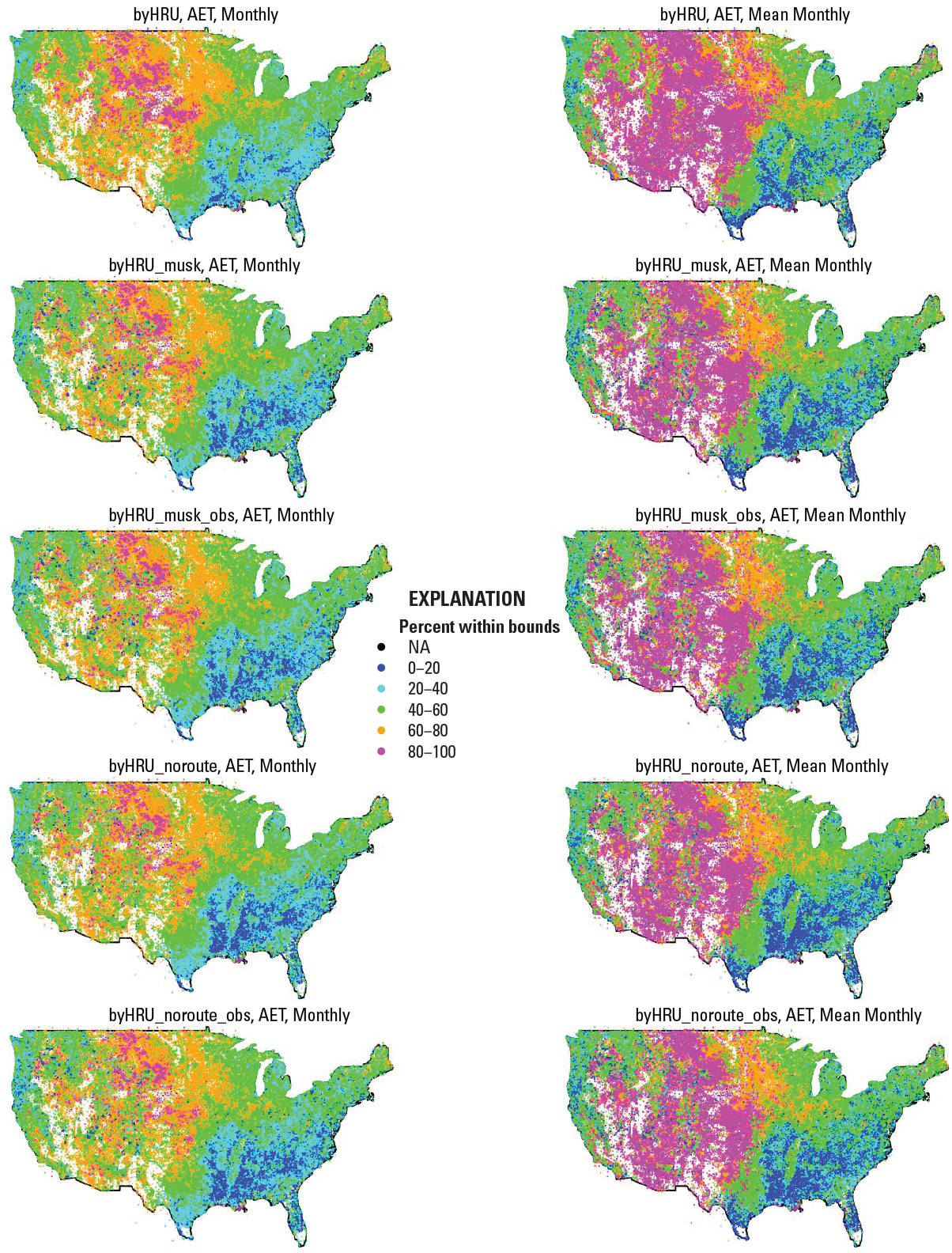
Maps showing percent of the time that simulated actual evapotranspiration (AET; Precipitation-Runoff Modeling System variable hru_actet) fell within the range of the measured AET baseline. The columns represent monthly and mean monthly AET baselines. The rows represent the byHRU, byHRU_musk, byHRU_musk_obs, byHRU_noroute, and byHRU_noroute_obs calibrations. A value of NA indicates that no comparison was made between simulated and measured values for that hydrologic response unit (HRU).
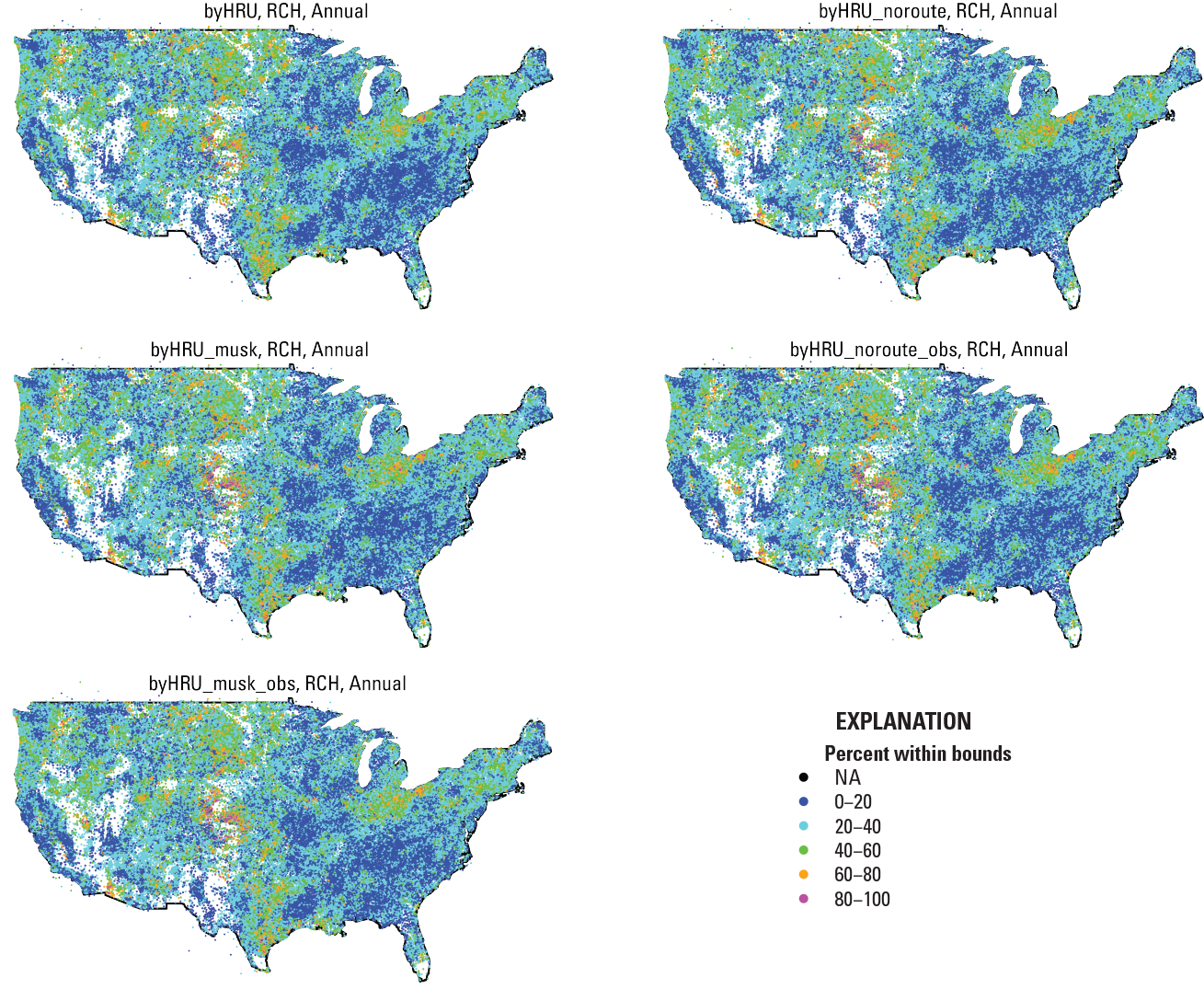
Maps showing percent of the time that simulated recharge (RCH; Precipitation-Runoff Modeling System variable recharge) fell within the range of the measured baseline. The columns represent annual RCH baselines. The column on the left represents the byHRU, byHRU_musk, and byHRU_musk_obs calibrations, and the column on the right represents the byHRU_noroute and byHRU_noroute_obs calibrations. A value of NA indicates that no comparison was made between simulated and measured values for that hydrologic response unit (HRU).
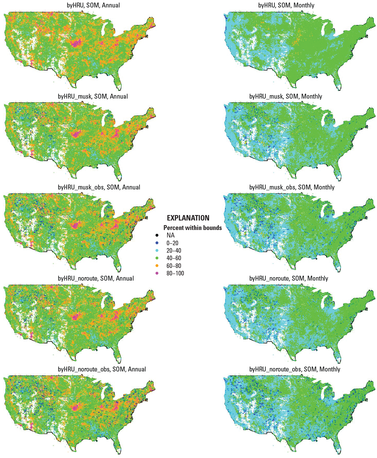
Maps showing percent of the time that simulated soil moisture (SOM; Precipitation-Runoff Modeling System variable soil_rechr) fell within the range of the measured baseline. The columns represent annual and monthly SOM baselines. The rows represent the byHRU, byHRU_musk, byHRU_musk_obs, byHRU_noroute, and byHRU_noroute_obs calibrations. A value of NA indicates that no comparison was made between simulated and measured values for that hydrologic response unit (HRU).
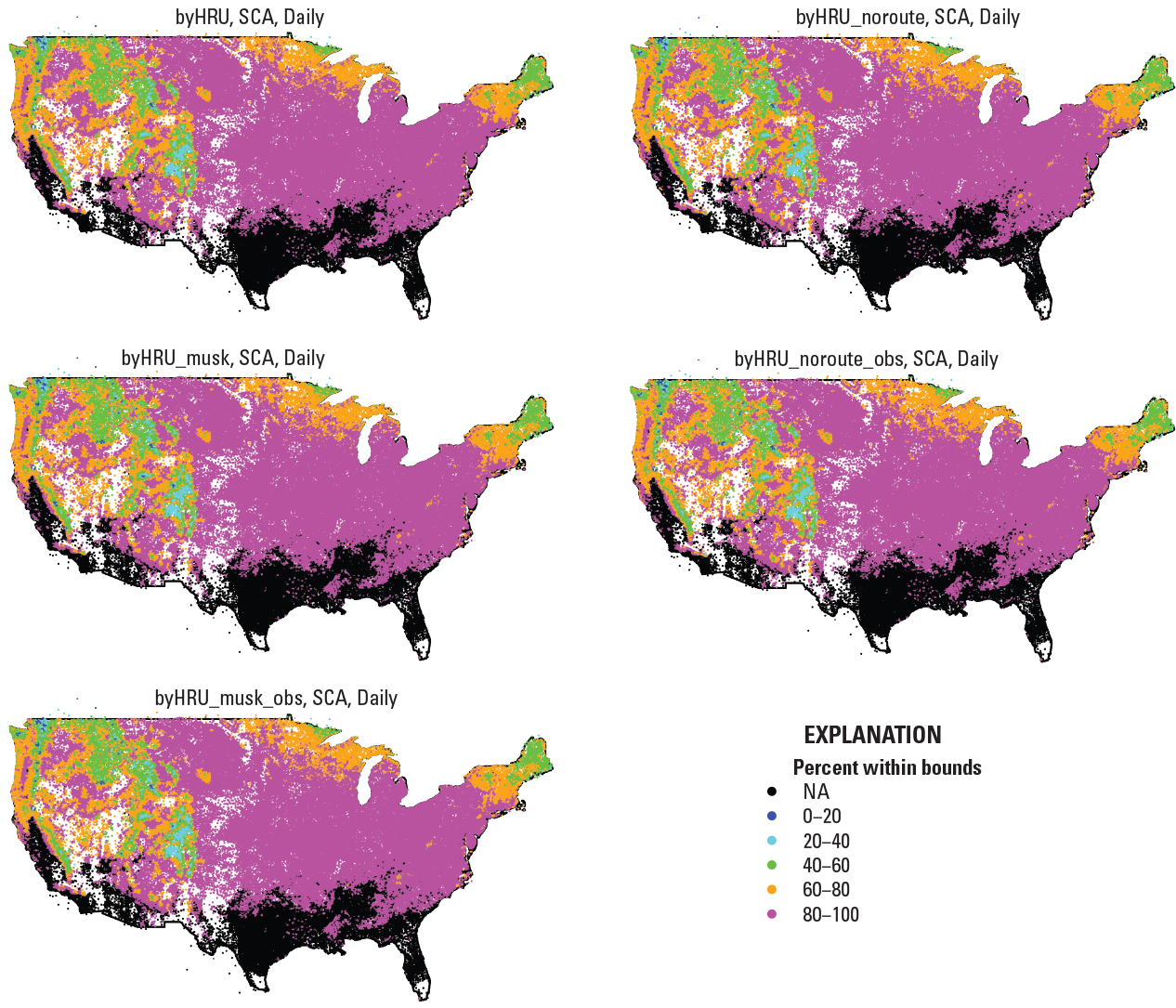
Maps showing percent of the time that simulated snow-covered area (SCA; Precipitation-Runoff Modeling System variable snowcov_area) fell within the range of the measured baseline. The columns represent daily SCA baselines. The column on the left represents the byHRU, byHRU_musk, and byHRU_musk_obs calibrations, and the column on the right represents the byHRU_noroute and byHRU_noroute_obs calibrations. A value of NA indicates that no comparison was made between simulated and measured values for that hydrologic response unit (HRU).
Comparisons Between Simulated and Measured Streamflow
A total of 8,270 streamgages were available in the NHM-PRMS model application based on those included in the GF (Viger and Bock, 2014). Of those 8,270 streamgages, 6,088 had a GF-based drainage area within 10 percent of the USGS published drainage area, and 1,336 were classified as reference-quality streamgages in the GAGES-II dataset (Falcone, 2011). The streamflow-simulation results were evaluated using the NSE (Nash and Sutcliffe, 1970; eq. 4 in this report). Spatial distributions of model performance using the NSE metric are shown for the 1,336 reference-quality and 4,752 non-reference-quality streamgage locations in figure 14 and figure 15, respectively. The NSE values were calculated using daily, log daily, and monthly streamflow for the byHRU, byHRU_musk, byHRU_musk_obs, byHRU_noroute, and byHRU_noroute_obs calibrations. The NSE value distributions shown in figure 14 and figure 15 are similar to (1) those shown by Newman and others (2015, fig. 5a of that report), in which a daily time-step hydrologic model was calibrated for 671 basins across the CONUS, and (2) those shown by Bock and others (2016, fig. 9a of that report), in which a monthly time-step hydrologic model was calibrated across the CONUS. This study, the Newman and others (2015) study, and the Bock and others (2016) study all indicated the poorest performing areas are generally in the central and southwestern United States. Newman and others (2015) attributed this to spatial variations in aridity and precipitation intermittency, contribution of snowmelt, and runoff seasonality.
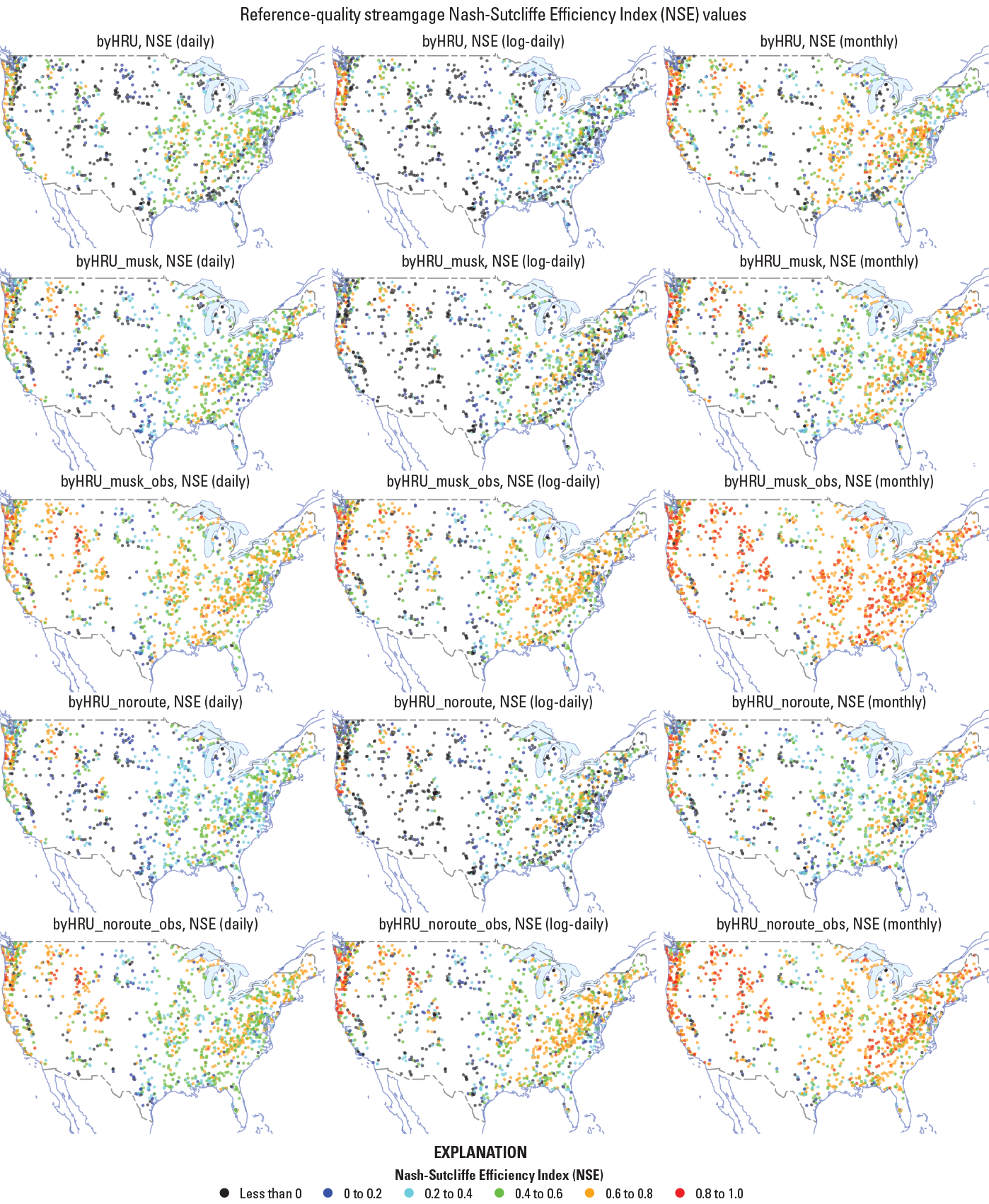
Maps showing Nash-Sutcliffe Efficiency Index (NSE) between observed and simulated streamflow at 1,336 reference-quality streamgages as defined by Falcone (2011). The columns represent NSE values calculated using daily, log of daily, and monthly values, respectively. The rows represent the byHRU, byHRU_musk, byHRU_musk_obs, byHRU_noroute, and byHRU_noroute_obs calibrations.
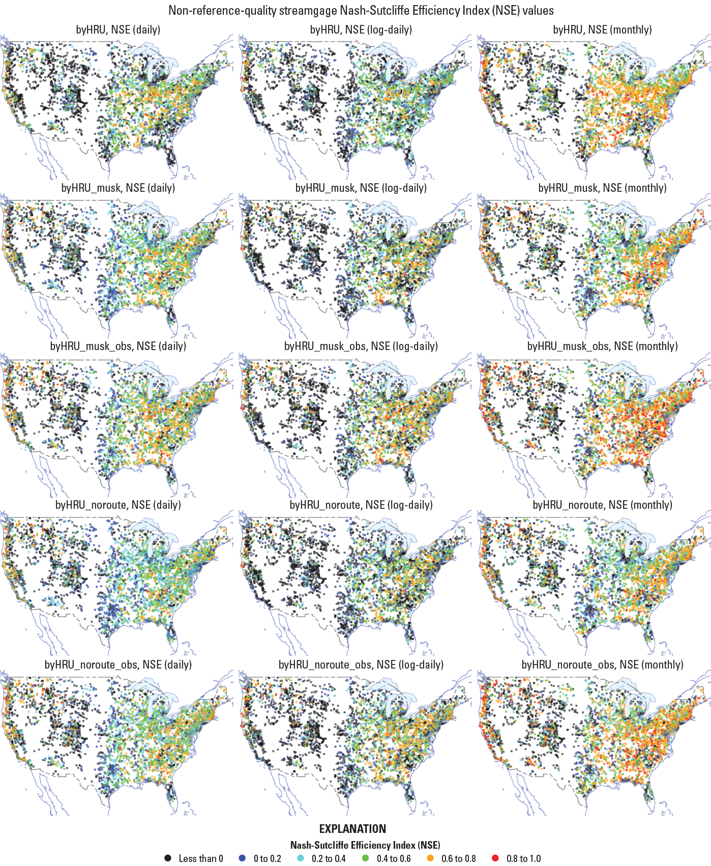
Maps showing Nash-Sutcliffe Efficiency Index (NSE) between observed and simulated streamflow at 4,752 non-reference-quality streamgages as defined by Falcone (2011). The columns represent NSE values calculated using daily, log of daily, and monthly values, respectively. The rows represent the byHRU, byHRU_musk, byHRU_musk_obs, byHRU_noroute, and byHRU_noroute_obs calibrations.
As expected, the NSE values improved as the calibration proceeded, due to the incorporation of statistically generated and observed streamflow datasets in the calibration. The non-reference-quality streamgages (fig. 15) tended to be affected by water use, flow regulation, or substantial urbanization. These streamgages are expected to have poorer performance compared to the reference-quality streamgages (fig. 14). However, both the reference-quality and non-reference-quality streamgage locations showed the same general pattern of performance across the CONUS, with some streamgage locations simulated by the NHM-PRMS quite well, especially for the monthly analysis. This could indicate that the timing and magnitude of streamflows on monthly time steps are not influenced as much by the water use and flow regulation as daily time-step streamflows and could be useful in monthly time-step calibrations in the future. Figure 16 summarizes the NSE values in figure 14 and figure 15 to percent exceedance curves for both the reference-quality and non-reference-quality streamgage locations for (A) daily, (B) log daily, and (C) monthly streamflow. When comparing the two routing procedures, continuity only and the Muskingum method, it was apparent that streamflow simulations benefit from the inclusion of explicit streamflow routing, with the byHRU_musk (blue) outperforming the byHRU_noroute (red) and the byHRU_musk_obs (green) outperforming the byHRU_noroute_obs (purple). The non-reference-quality streamgage locations tended to be affected by anthropogenic factors; examples include water use, flow regulation, or substantial urbanization. The non-reference-quality streamgages were expected to have poorer performance compared to the reference-quality streamgages.
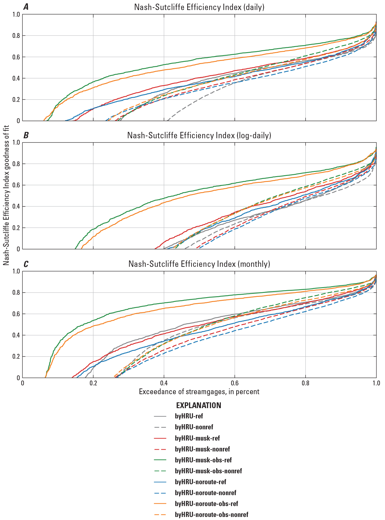
Graphs showing summary of Nash-Sutcliffe Efficiency Index between observed and simulated streamflow at reference-quality and non-reference-quality streamgages as defined by Falcone (2011) using: A, daily; B, log of daily; and C, monthly streamflow values.
Limitations of NHM-PRMS Modeling Application
The PRMS model application that was developed as part of the NHM infrastructure provided simulations of streamflow and other water-budget components of the hydrologic cycle. The report by LaFontaine and others (2019) discussed some of the limitations associated with the calibration strategy used in this study. As with any hydrologic modeling application, the assumptions and simplifications inherent in the representation of the physical processes limited the accuracy and applicability of the results. This is typical for a watershed model such as PRMS, which is a combination of process-based theoretical and empirical equations that are used to simulate the hydrologic cycle. The following discussion highlights some of those limitations that are applicable at the CONUS scale.
The calibration methodology used for this study was intended to provide an initial set of spatially distributed parameters that represented a consistent hydrologic response across the CONUS and from which users could subset for local applications which could be improved with local datasets. There was a limited coverage of reference-quality streamflow information available in the CONUS (Kiang and others, 2013). Areas not upstream from reference-quality streamgages were therefore not as easily calibrated or evaluated. The calibration methodology presented in this study couples the calibration of both gaged and ungaged areas, with the initial parameters for the model application adjusted together to maintain their spatial distribution. This approach to calibration, with its focus on regional similarity, was previously used by Bock and others (2016) in the development of a national-scale application of the MWBM (McCabe and Markstrom, 2007) as part of the NHM infrastructure (Regan and others, 2018). Routing parameters for stream segments downstream of the headwater watersheds were not calibrated. HRUs connected to those stream segments were calibrated during the byHRU calibration step, but, due to extensive anthropogenic effects to streamflow data in larger watersheds, this natural- flows application of the NHM-PRMS did not incorporate those data into the calibration. If naturalized flow data were developed for those non-reference locations, or if additional simulation capabilities were incorporated into the NHM-PRMS application (such as reservoir operations or water-use effects), perhaps those areas of the model domain could be calibrated. However, such improvements were beyond the scope of this study.
The calibration methodology used for this study used several types of hydrologic information (measured streamflow, simulated streamflow, runoff, actual evapotranspiration, recharge, soil moisture, and snow-covered area) to optimize the NHM-PRMS model parameters. As improved or additional datasets become available at the national scale (for example, remotely sensed soil moisture), that information could also be used to better constrain the parameter-optimization scheme beyond its current capabilities and to apply the model to more parts of the hydrologic cycle. For example, current representations of soil moisture and recharge in the baseline datasets were limited to normalized distributions of monthly and annual values; this was due to different ways in which the observation datasets and the PRMS model structure conceptualize those fluxes and storages. The magnitude of the error bounds associated with several of the baseline datasets did not constrain the calibration procedure as much as desired. Wider error bounds allowed for a larger number of parameter sets to meet the objective function criteria, which lead to equifinality issues. By improving understanding and quantification of the baseline dataset targets and the associated error bounds, the calibration procedure can be further constrained beyond its current capabilities.
Water-use data at the CONUS scale were not available for use in this study. LaFontaine and others (2017) incorporated monthly estimates of site-specific surface-water withdrawals and return flow, and of groundwater withdrawals in the southeastern United States. When available, time series of water-use information should be incorporated to allow modeling simulations to better represent the actual hydrologic cycle for a particular study area instead of just the natural hydrologic response to climate and land-cover conditions. These water-use estimates could either be incorporated into the baseline dataset observations to make them more “natural” or they could be directly incorporated into the model simulations during calibration using the PRMS Water Use module (Regan and LaFontaine, 2017).
The streamflow simulations developed in this study did not include the effects of flow regulation (for example, dam operations) on hydrologic response. The PRMS provided the ability to include lakes in the stream routing process (Regan and LaFontaine, 2017), but not the complex rule-curve-based methodologies such as those used by the U.S. Army Corps of Engineers. One option within the PRMS allowed for the replacement of simulated streamflow with observed streamflow at the dam location. This option may be useful for historical simulations targeting actual streamflows, but it did not preserve the water balance and did not help for projecting future hydrologic response. Other options included coupling the PRMS with software packages specifically built to deal with water management such as HEC-ResSim (https://www.hec.usace.army.mil/software/hec-ressim/) (U.S. Army Corps of Engineers Hydrologic Engineering Center, 2013) or MODSIM-DSS (http://modsim.engr.colostate.edu/modsim.php) (Colorado State University, 2017).
Summary
This report describes a procedure that provides informative baseline datasets for the conterminous United States (CONUS) for model calibration and evaluation beyond streamflow, using both the U.S. Geological Survey National Hydrologic Model (NHM) infrastructure application of the Precipitation-Runoff Modeling System (PRMS) and a new routing module based on the Muskingum method. The new routing module, muskingum_mann, is based on the current PRMS routing module muskingum and computes the routing coefficients from stream-channel characteristics instead of being directly specified in the parameter file. The baseline CONUS-scale datasets were derived with error bounds for runoff, actual evapotranspiration, recharge, soil moisture, and snow-covered area. The corresponding process variables from the model were examined in a CONUS-scale three-part calibration procedure that considers volume (calibration by hydrologic response unit [byHRU]), timing (calibration by headwater watershed [byHW]), and observed streamflow (byHWobs). The various levels of calibration were evaluated against observed streamflow datasets for the CONUS. The simulations best represented streamflow in the eastern United States and the U.S. Pacific Northwest. The simulations did not represent streamflow as well in the central and southwestern United States.
The calibration methodology presented here is meant to give users a starting place for model application. Using a variety of alternative datasets for calibration of the water budget provides users of the NHM-PRMS with spatially distributed initial parameters suitable for application at the local level. The Bandit software can extract NHM-PRMS model subsets for any watershed in the CONUS domain, providing users with local models with realistic parameters. These extractions can then be calibrated to improve the match between simulations and a single measured streamflow time series compared to the current model calibration. Using a variety of alternative datasets for calibration of the water budget helps alleviate the equifinality problem (getting the right answer for the wrong reason). An improved and expanded understanding of these alternative data products, provided in a readily available way, could facilitate modeling communities in the calibration and evaluation of hydrologic models using more than streamflow.
Acknowledgments
This study was made possible through the Water Availability and Use Science Program under the direction of Melinda Dalton. The authors are grateful for the thorough technical reviews provided by Adel Haj (U.S. Geological Survey) and Eric Swain (U.S. Geological Survey), which have strengthened the final manuscript.
References Cited
Beven, K., and Binley, A., 1992, The future of distributed models—Model calibration and uncertainty prediction: Hydrological Processes, v. 6, no. 3, p. 279–298, accessed September 29, 2019, at https://doi.org/10.1002/hyp.3360060305.
Beven, K., and Freer, J., 2001, Equifinality, data assimilation, and uncertainty estimation in mechanistic modelling of complex environmental systems using the GLUE methodology: Journal of Hydrology, v. 249, no. 1-4, p. 11–29, accessed September 27, 2019, at https://doi.org/10.1016/S0022-1694(01)00421-8.
Blodgett, D.L., Booth, N.L., Kunicki, T.C., Walker, J.I., and Viger, R.J., 2011, Description and testing of the Geo Data Portal—Data integration framework and Web processing services for environmental science collaboration: U.S. Geological Survey Open-File Report 2011–1157, 9 p., accessed March 2, 2017, at https://doi.org/10.3133/ofr20111157.
Bock, A.R., Farmer, W.H., and Hay, L.E., 2018, Quantifying uncertainty in simulated streamflow and runoff from a continental-scale monthly water balance model: Advances in Water Resources, v. 122, p. 166–175, accessed August 20, 2019, at https://doi.org/10.1016/j.advwatres.2018.10.005.
Bock, A.R., Hay, L.E., Markstrom, S.L., Emmerich, C., and Talbert, M., 2017, The U.S. Geological Survey monthly water balance model futures portal: U.S. Geological Survey Open-File Report 2016–1212, 21 p., accessed August 20, 2019, at https://doi.org/10.3133/ofr20161212.
Bock, A.R., Hay, L.E., McCabe, G.J., Markstrom, S.L., and Atkinson, R.D., 2016, Parameter regionalization of a monthly water balance model for the conterminous United States: Hydrology and Earth System Sciences, v. 20, no. 7, p. 2861–2876, accessed June 4, 2018, at https://doi.org/10.5194/hess-20-2861-2016.
Bourgin, F., Andréassian, V., Perrin, C., and Oudin, L., 2015, Transferring global uncertainty estimates from gauged to ungauged catchments: Hydrology and Earth System Sciences, v. 19, no. 5, p. 2535–2546, accessed September 29, 2019, at https://doi.org/10.5194/hess-19-2535-2015.
Campo, L., Caparrini, F., and Castelli, F., 2006, Use of multi-platform, multi-temporal remote-sensing data for calibration of a distributed hydrological model—An application in the Arno basin, Italy: Hydrological Processes, v. 20, no. 13, p. 2693–2712, accessed September 29, 2019, at https://doi.org/10.1002/hyp.6061.
Cao, W., Sun, G., McNulty, S.G., Chen, J., Noormets, A., Skaggs, R.W., and Amatya, D.M., 2006, Evapotranspiration of a mid-rotation loblolly pine plantation and a recently harvested stands on the coastal plain of North Carolina, U.S.A., in Williams, T., ed., Hydrology and management of forested wetlands—Proceedings of the International Conference: St. Joseph, Mich., American Society of Agricultural and Biological Engineers, p. 27–33, accessed January 30, 2017, at https://www.fs.usda.gov/treesearch/pubs/22421.
Chavarria, S.G., Moeser, C.D., and Douglas-Mankin, K.R., 2020, Application of the Precipitation-Runoff Modeling System (PRMS) to simulate near-native streamflow in the Upper Rio Grande Basin: U.S. Geological Survey Scientific Investigations Report 2020–5026, 48 p., accessed February 1, 2021, at https://doi.org/10.3133/sir20205026.
Colorado State University, 2017, MODSIM-DSS: Colorado State University, MODSIM website, accessed September 25, 2019, at http://modsim.engr.colostate.edu/modsim.php.
Cukier, R.I., Fortuin, C.M., Shuler, K.E., Petschek, A.G., and Schaibly, J.H., 1973, Study of the sensitivity of coupled reaction systems to uncertainties in rate coefficients. I Theory: The Journal of Chemical Physics, v. 59, no. 8, p. 3873–3878, accessed October 27, 2017, at https://doi.org/10.1063/1.1680571.
Cukier, R.I., Schaibly, J.H., and Shuler, K.E., 1975, Study of the sensitivity of coupled reaction systems to uncertainties in rate coefficients. III. Analysis of the approximations: The Journal of Chemical Physics, v. 63, no. 3, p. 1140–1149, accessed October 27, 2017, at https://doi.org/10.1063/1.431440.
Döll, P., Müller Schmied, H., Schuh, C., Portmann, F.T., and Eicker, A., 2014, Global-scale assessment of groundwater depletion and related groundwater abstractions—Combining hydrological modeling with information from well observations and GRACE satellites: Water Resources Research, v. 50, no. 7, p. 5698–5720, accessed September 29, 2019, at https://doi.org/10.1002/2014WR015595.
Driscoll, J.M., Markstrom, S.L., Regan, R.S., Hay, L.E., and Viger, R.J., 2017, National Hydrologic Model Parameter Database—2017-05-08 download: U.S. Geological Survey database, accessed September 24, 2017, at https://doi.org/10.5066/F7NS0SCW.
Duan, Q.Y., Gupta, V.K., and Sorooshian, S., 1993, Shuffled complex evolution approach for effective and efficient global minimization: Journal of Optimization Theory and Applications, v. 76, no. 3, p. 501–521, accessed November 3, 2017, at https://doi.org/10.1007/BF00939380.
Duan, Q., Sorooshian, S., and Gupta, V., 1992, Effective and efficient global optimization for conceptual rainfall-runoff models: Water Resources Research, v. 28, no. 4, p. 1015–1031, accessed September 2, 2009, at https://doi.org/10.1029/91WR02985.
Duan, Q., Sorooshian, S., and Gupta, V.K., 1994, Optimal use of the SCE-UA global optimization method for calibrating watershed models: Journal of Hydrology, v. 158, no. 3-4, p. 265–284, accessed September 2, 2009, at https://doi.org/10.1016/0022-1694(94)90057-4.
Falcone, J., 2011, GAGES–II, Geospatial attributes of gages for evaluating streamflow: U.S. Geological Survey dataset, accessed October 18, 2017, at https://water.usgs.gov/GIS/metadata/usgswrd/XML/gagesII_Sept2011.xml.
Farmer, W.H., 2016, Ordinary kriging as a tool to estimate historical daily streamflow records: Hydrology and Earth System Sciences, v. 20, no. 7, p. 2721–2735, accessed September 27, 2017, at https://doi.org/10.5194/hess-20-2721-2016.
Farmer, W.H., LaFontaine, J.H., and Hay, L.E., 2019, Calibration of the US Geological Survey National Hydrologic Model in Ungauged Basins Using Statistical At-Site Streamflow Simulations: Journal of Hydrologic Engineering, v. 24, no. 11, p. 04019049, accessed September 29, 2019, at https://doi.org/10.1061/(ASCE)HE.1943-5584.0001854.
Farmer, W.H., and Vogel, R.M., 2016, On the deterministic and stochastic use of hydrologic models: Water Resources Research, v. 52, no. 7, p. 5619–5633, accessed September 25, 2019, at https://doi.org/10.1002/2016WR019129.
Franz, K.J., and Karsten, L.R., 2013, Calibration of a distributed snow model using MODIS snow covered area data: Journal of Hydrology, v. 494, p. 160–175, accessed January 27, 2017, at https://doi.org/10.1016/j.jhydrol.2013.04.026.
Hall, D.K., and Riggs, G.A., 2016, MODIS/Terra snow cover daily L3 global 0.05Deg CMG, Version 6: Boulder, Colo., National Snow and Ice Data Center, accessed September 27, 2019, at https://doi.org/10.5067/MODIS/MOD10C1.006.
Hay, L.E., and LaFontaine, J.H., 2020, Application of the National Hydrologic Model Infrastructure with the Precipitation-Runoff Modeling System (NHM-PRMS), 1980‒2016, Daymet Version 3 calibration: U.S. Geological Survey data release, accessed June 1, 2020, at https://doi.org/10.5066/P9PGZE0S.
Hay, L.E., Leavesley, G.H., and Clark, M.P., 2006a, Use of remotely sensed snow-covered area in watershed model calibration for the Sprague River, Oregon, in Joint 8th Federal Interagency Sedimentation Conference and 3rd Federal Interagency Hydrologic Modeling Conference, Reno, Nev., April 2–6, 2006, Proceedings: Subcommittee on Hydrology, 8 p., accessed September 29, 2019, at https://acwi.gov/hydrology/mtsconfwkshops/conf_proceedings/3rdFIHMC/7D_Hay.pdf.
Hay, L.E., Leavesley, G.H., Clark, M.P., Markstrom, S.L., Viger, R.J., and Umemoto, M., 2006b, Step wise, multiple objective calibration of a hydrologic model for a snowmelt dominated basin: Journal of the American Water Resources Association, v. 42, no. 4, p. 877–890, accessed August 29, 2019, at https://doi.org/10.1111/j.1752-1688.2006.tb04501.x.
Hay, L., Norton, P., Viger, R., Markstrom, S., Steven Regan, R., and Vanderhoof, M., 2018, Modelling surface-water depression storage in a Prairie Pothole Region: Hydrological Processes, v. 32, no. 4, p. 462–479, accessed September 28, 2019, at https://doi.org/10.1002/hyp.11416.
Hay, L.E., and Umemoto, M., 2007, Multiple-objective stepwise calibration using Luca: U.S. Geological Survey Open-File Report 2006–1323, 25 p., accessed September 29, 2019, at https://doi.org/10.3133/ofr20061323.
Immerzeel, W.W., and Droogers, P., 2008, Calibration of a distributed hydrological model based on satellite evapotranspiration: Journal of Hydrology, v. 349, no. 3-4, p. 411–424, accessed January 30, 2017, at https://doi.org/10.1016/j.jhydrol.2007.11.017.
Isenstein, E.M., Wi, S., and Yang, Y.C.E., 2015, Calibration of a distributed hydrologic model using streamflow and remote sensing snow data, in World Environmental and Water Resources Congress 2015, Austin, Tex., May 17–21, 2015, Proceedings: American Society of Civil Engineers, p. 973–982, accessed October 27, 2017, at https://doi.org/10.1061/9780784479162.093.
Kiang, J.E., Stewart, D.W., Archfield, S.A., Osborne, E.B., and Eng, K., 2013, A national streamflow network gap analysis: U.S. Geological Survey Scientific Investigations Report 2013–5013, 79 p. plus one appendix as a separate file, accessed September 29, 2019, at https://doi.org/10.3133/sir20135013.
Koren, V., Moreda, F., and Smith, M., 2008, Use of soil moisture observations to improve parameter consistency in watershed calibration: Physics and Chemistry of the Earth Parts A/B/C, v. 33, no. 17-18, p. 1068–1080, accessed January 27, 2017, at https://doi.org/10.1016/j.pce.2008.01.003.
Kuppel, S., Tetzlaff, D., Maneta, M.P., and Soulsby, C., 2018, EcH<sub>2</sub>O-iso 1.0—Water isotopes and age tracking in a process-based, distributed ecohydrological model: Geoscientific Model Development, v. 11, no. 7, p. 3045–3069, accessed September 29, 2019, at https://doi.org/10.5194/gmd-11-3045-2018.
LaFontaine, J.H., Hart, R.M., Hay, L.E., Farmer, W.H., Bock, A.R., Viger, R.J., Markstrom, S.L., Regan, R.S., and Driscoll, J.M., 2019, Simulation of water availability in the Southeastern United States for historical and potential future climate and land-cover conditions: U.S. Geological Survey Scientific Investigations Report 2019–5039, 83 p., accessed September 19, 2019, at https://doi.org/10.3133/sir20195039.
LaFontaine, J.H., Hay, L.E., Viger, R.J., Markstrom, S.L., Regan, R.S., Elliott, C.M., and Jones, J.W., 2013, Application of the Precipitation-Runoff Modeling System (PRMS) in the Apalachicola-Chattahoochee-Flint River Basin in the southeastern United States: U.S. Geological Survey Scientific Investigations Report 2013–5162, 118 p., accessed September 27, 2016, at https://doi.org/10.3133/sir20135162.
LaFontaine, J.H., Hay, L.E., Viger, R.J., Regan, R.S., and Markstrom, S.L., 2015, Effects of climate and land cover on hydrology in the southeastern U.S.—Potential impacts on watershed planning: Journal of the American Water Resources Association, v. 51, no. 5, p. 1235–1261, accessed August 23, 2019, at https://doi.org/10.1111/1752-1688.12304.
LaFontaine, J.H., Jones, L.E., and Painter, J.A., 2017, Simulations of hydrologic response in the Apalachicola-Chattahoochee-Flint River Basin, southeastern United States: U.S. Geological Survey Scientific Investigations Report 2017–5133, 112 p., accessed September 25, 2019, at https://doi.org/10.3133/sir20175133.
Li, Y., Grimaldi, S., Pauwels, V.R.N., and Walker, J.P., 2018, Hydrologic model calibration using remotely sensed soil moisture and discharge measurements—The impact on predictions at gauged and ungauged locations: Journal of Hydrology, v. 557, p. 897–909, accessed September 30, 2019, at https://doi.org/10.1016/j.jhydrol.2018.01.013.
Li, Y., Grimaldi, S., Walker, J.P., and Pauwels, V.R.N., 2016, Application of remote sensing data to constrain operational rainfall-driven flood forecasting—A review: Remote Sensing, v. 8, no. 6, 29 p., accessed September 30, 2019, at https://doi.org/10.3390/rs8060456.
Markstrom, S.L., 2012, P2S—Coupled simulation with the Precipitation-Runoff Modeling System (PRMS) and the Stream Temperature Network (SNTemp) Models: U.S. Geological Survey Open-File Report 2012–1116, 19 p., accessed August 23, 2019, at https://doi.org/10.3133/ofr20121116.
Markstrom, S.L., Hay, L.E., and Clark, M.P., 2016, Towards simplification of hydrologic modeling—Identification of dominant processes: Hydrology and Earth System Sciences, v. 20, no. 11, p. 4655–4671, accessed February 9, 2017. https://doi.org/10.5194/hess-20-4655-2016.
Markstrom, S.L., Regan, R.S., Hay, L.E., Viger, R.J., Webb, R.M.T., Payn, R.A., and LaFontaine, J.H., 2015, PRMS-IV, the precipitation-runoff modeling system, version 4: U.S. Geological Survey Techniques and Methods, book 6, chap. B7, 158 p., accessed August 20, 2019, at https://doi.org/10.3133/tm6B7.
Mastin, M.C., and Vaccaro, J.J., 2002, Documentation of Precipitation-Runoff Modeling System modules for the Modular Modeling System modified for the Watershed and River Systems Management Program: U.S. Geological Survey Open-File Report 2002–362, 5 p., accessed September 30, 2019, at https://doi.org/10.3133/ofr02362.
McCabe, G.J., and Markstrom, S.L., 2007, A monthly water-balance model driven by a graphical user interface: U.S. Geological Survey Open-File Report 2007–1088, 6 p., accessed October 27, 2017, at https://doi.org/10.3133/ofr20071088.
Nash, J.E., and Sutcliffe, J.V., 1970, River flow forecasting through conceptual models part I—A discussion of principles: Journal of Hydrology, v. 10, no. 3, p. 282–290, accessed September 2, 2009, at https://doi.org/10.1016/0022-1694(70)90255-6.
Newman, A.J., Clark, M.P., Sampson, K., Wood, A., Hay, L.E., Bock, A., Viger, R.J., Blodgett, D., Brekke, L., Arnold, J.R., Hopson, T., and Duan, Q., 2015, Development of a large-sample watershed-scale hydrometeorological data set for the contiguous USA—Data set characteristics and assessment of regional variability in hydrologic model performance: Hydrology and Earth System Sciences, v. 19, no. 1, p. 209–223, accessed August 20, 2019, at https://doi.org/10.5194/hess-19-209-2015.
Pfannerstill, M., Bieger, K., Guse, B., Bosch, D.D., Fohrer, N., and Arnold, J.G., 2017, How to Constrain Multi-Objective Calibrations of the SWAT Model Using Water Balance Components: Journal of the American Water Resources Association, v. 53, no. 3, p. 532–546, accessed September 30, 2019, at https://doi.org/10.1111/1752-1688.12524.
Refsgaard, J.C., 1997, Parameterisation, calibration and validation of distributed hydrological models: Journal of Hydrology, v. 198, no. 1-4, p. 69–97, accessed February 9, 2017, at https://doi.org/10.1016/S0022-1694(96)03329-X.
Regan, R.S., Juracek, K.E., Hay, L.E., Markstrom, S.L., Viger, R.J., Driscoll, J.M., LaFontaine, J.H., and Norton, P.A., 2019, The U. S. Geological Survey National Hydrologic Model infrastructure—Rationale, description, and application of a watershed-scale model for the conterminous United States: Environmental Modelling & Software, v. 111, p. 192–203, accessed September 13, 2019. https://doi.org/10.1016/j.envsoft.2018.09.023.
Regan, R.S., and LaFontaine, J.H., 2017, Documentation of the dynamic parameter, water-use, stream and lake flow routing, and two summary output modules and updates to surface-depression storage simulation and initial conditions specification options with the Precipitation-Runoff Modeling System (PRMS): U.S. Geological Survey Techniques and Methods, book 6, chap. B8, 60 p., accessed October 27, 2017, at https://doi.org/10.3133/tm6B8.
Regan, R.S., Markstrom, S.L., Hay, L.E., Viger, R.J., Norton, P.A., Driscoll, J.M., and LaFontaine, J.H., 2018, Description of the National Hydrologic Model for use with the Precipitation-Runoff Modeling System (PRMS): U.S. Geological Survey Techniques and Methods, book 6, chap B9, 38 p., accessed August 20, 2019, at https://doi.org/10.3133/tm6B9.
Reitz, M., Sanford, W.E., Senay, G.B., and Cazenas, J., 2017, Annual estimates of recharge, quick-flow runoff, and evapotranspiration for the contiguous U.S. using empirical regression equations: Journal of the American Water Resources Association, v. 53, no. 4, p. 961–983, accessed September 19, 2019, at https://doi.org/10.1111/1752-1688.12546.
Reusser, D.E., Buytaert, W., and Zehe, E., 2011, Temporal dynamics of model parameter sensitivity for computationally expensive models with the Fourier Amplitude Sensitivity Test: Water Resources Research, v. 47, no. 7, 15 p., accessed September 25, 2019, at https://doi.org/10.1029/2010WR009947.
Rientjes, T.H.M., Muthuwatta, L.P., Bos, M.G., Booij, M.J., and Bhatti, H.A., 2013, Multi-variable calibration of a semi-distributed hydrological model using streamflow data and satellite-based evapotranspiration: Journal of Hydrology, v. 505, p. 276–290, accessed January 30, 2017, at https://doi.org/10.1016/j.jhydrol.2013.10.006.
Risley, J.C., 2019, Using the Precipitation-Runoff Modeling System to predict seasonal water availability in the upper Klamath River basin, Oregon and California: U.S. Geological Survey Scientific Investigations Report 2019–5044, 37 p., accessed July 1, 2021, at https://doi.org/10.3133/sir20195044.
Romano, N., 2014, Soil moisture at local scale—Measurements and simulations: Journal of Hydrology, v. 516, p. 6–20, accessed September 30, 2019, at https://doi.org/10.1016/j.jhydrol.2014.01.026.
Rosa, S.N., and Hay, L.E., 2019, Fena Valley Reservoir watershed and water-balance model updates and expansion of watershed modeling to southern Guam (ver. 1.1, February 2019): U.S. Geological Survey Scientific Investigations Report 2017–5093, 64 p., accessed August 27, 2019, at https://doi.org/10.3133/sir20175093.
Saltelli, A., Ratto, M., Tarantola, S., and Campolongo, F., 2006, Sensitivity analysis practices—Strategies for model-based inference: Reliability Engineering & System Safety, v. 91, no. 10-11, p. 1109–1125, accessed September 30, 2019, at https://doi.org/10.1016/j.ress.2005.11.014.
Santanello, J.A., Jr., Peters-Lidard, C.D., Garcia, M.E., Mocko, D.M., Tischler, M.A., Moran, M.S., and Thoma, D.P., 2007, Using remotely-sensed estimates of soil moisture to infer soil texture and hydraulic properties across a semi-arid watershed: Remote Sensing of Environment, v. 110, no. 1, p. 79–97, accessed January 27, 2017, at https://doi.org/10.1016/j.rse.2007.02.007.
Schaibly, J.H., and Shuler, K.E., 1973, Study of the sensitivity of coupled reaction systems to uncertainties in rate coefficients. II Applications: The Journal of Chemical Physics, v. 59, no. 8, p. 3879–3888, accessed September 30, 2019, at https://doi.org/10.1063/1.1680572.
Senay, G.B., Bohms, S., Singh, R.K., Gowda, P.H., Velpuri, N.M., Alemu, H., and Verdin, J.P., 2013, Operational Evapotranspiration Mapping Using Remote Sensing and Weather Datasets—A New Parameterization for the SSEB Approach: Journal of the American Water Resources Association, v. 49, no. 3, p. 577–591, accessed August 23, 2019, at https://doi.org/10.1111/jawr.12057.
The Nature Conservancy, 2009, Indicators of hydrologic alteration, version 7.1—User’s manual: The Nature Conservancy, accessed November 3, 2017, at https://www.conservationgateway.org/ConservationPractices/Freshwater/EnvironmentalFlows/MethodsandTools/IndicatorsofHydrologicAlteration/Documents/IHA V7.pdf.
Thornton, P.E., Thornton, M.M., Mayer, B.W., Wei, Y., Devarakonda, R., Vose, R.S., and Cook, R.B., 2017, Daymet—Daily surface weather data on a 1-km grid for North America, version 3: Oak Ridge, Tenn., Oak Ridge National Library Distributed Active Archive Center, accessed August 20, 2019, at https://doi.org/10.3334/ORNLDAAC/1328.
Thorstensen, A., Nguyen, P., Hsu, K., and Sorooshian, S., 2016, Using Densely Distributed Soil Moisture Observations for Calibration of a Hydrologic Model: Journal of Hydrometeorology, v. 17, no. 2, p. 571–590, accessed September 30, 2019, at https://doi.org/10.1175/JHM-D-15-0071.1.
U.S. Army Corps of Engineers Hydrologic Engineering Center, 2013, HEC-ResSim (Reservoir System Simulation) software, ver. 3.1: U.S. Army Corps of Engineers Hydrologic Engineering Center website, accessed September 25, 2019, at https://www.hec.usace.army.mil/software/hec-ressim/.
Van Beusekom, A.E., Hay, L.E., Viger, R.J., Gould, W.A., Collazo, J.A., and Khalyani, A.H., 2014, The effects of changing land cover on streamflow simulation in Puerto Rico: Journal of the American Water Resources Association, v. 50, no. 6, p. 1575–1593, accessed August 22, 2019, at https://doi.org/10.1111/jawr.12227.
Van Beusekom, A.E., and Viger, R.J., 2018, A physically based daily simulation of the glacier‐dominated hydrology of the Copper River Basin, Alaska: Water Resources Research, v. 54, no. 7, p. 4983–5000, accessed September 5, 2019, at https://doi.org/10.1029/2018WR022625.
Viger, R.J., 2014, Preliminary spatial parameters for PRMS based on the Geospatial Fabric, NLCD2001 and SSURGO: U.S. Geological Survey data release, accessed September 16, 2016, at https://doi.org/10.5066/F7WM1BF7.
Viger, R.J., and Bock, A., 2014, GIS features of the Geospatial Fabric for national hydrologic modeling: U.S. Geological Survey data release, accessed September, 16, 2016, at https://doi.org/10.5066/F7542KMD.
Viger, R.J., Hay, L.E., Markstrom, S.L., Jones, J.W., and Buell, G.R., 2011, Hydrologic effects of urbanization and climate change on the Flint River Basin, Georgia: Earth Interactions, v. 15, no. 20, p. 1–25, accessed October 17, 2017, at https://doi.org/10.1175/2010EI369.1.
Viger, R.J., and Leavesley, G.H., 2007, Section 4—The GIS Weasel user’s manual: U.S. Geological Survey Techniques and Methods, book 6, chap. B4, 201 p., accessed September 24, 2017, at https://doi.org/10.3133/tm6B4.
Wanders, N., Karssenberg, D., de Roo, A., de Jong, S.M., and Bierkens, M.F.P., 2014, The suitability of remotely sensed soil moisture for improving operational flood forecasting: Hydrology and Earth System Sciences, v. 18, no. 6, p. 2343–2357, accessed January 27, 2017. https://doi.org/10.5194/hess-18-2343-2014.
Appendix 1. National Hydrologic Model Infrastructure Application of the Precipitation-Runoff Modeling System (NHM-PRMS) Calibration Setup
Introduction
This appendix describes in detail the necessary file and directory structure for the three-part calibration procedure using the U.S. Geological Survey (USGS) National Hydrologic Model (NHM) infrastructure application of the Precipitation-Runoff Modeling System (PRMS; Regan and others, 2018, 2019). The three-part calibration procedure considers volume (calibration by hydrologic response unit [byHRU]), timing (calibration by headwater watershed [byHW]), and observed streamflow (byHWobs). The calibration procedure uses five non-streamflow data products (runoff, actual evapotranspiration, recharge, soil moisture, and snow-covered area), statistically based streamflow simulations, and observed streamflow as calibration targets. A multiple-objective, stepwise, automated calibration procedure was used to identify the optimal set of parameters for each calibration step. This appendix describes the file and directory structure needed to run this calibration technique using the provided code and supporting data available in Hay and LaFontaine (2020).
Calibration of the PRMS Application of the NHM
A three-part procedure was used to calibrate the NHM-PRMS for the conterminous United States (CONUS): by hydrologic response unit (HRU), by headwater watershed, and including observed streamflow. The following sections describe the file and directory structure needed to run each of the three calibration steps. These programs were designed to run on a Linux system. The results of this calibration workflow and the described computer programs files are documented in Hay and LaFontaine (2020).
Part 1: Calibration by Hydrologic Response Unit (byHRU calibration)
The byHRU calibration is used to calibrate each HRU individually. The following sections demonstrate how to calibrate one HRU, but this methodology is meant to calibrate the approximately 110,000 HRUs in this model application simultaneously. The main text of this report documents the results of the byHRU calibration for a CONUS-scale application of the NHM-PRMS for 109,951 HRUs. The byHRU calibration is considered a water-balance volume calibration which uses non-streamflow data products as calibration targets to calibrate an HRU. Table 1.1 lists the necessary files for calibrating one HRU with the byHRU procedure.
Table 1.1.
Files needed for the byHRU calibration procedure.[AET, actual evapotranspiration; MWBM, Monthly Water Balance Model; MOD16, MODIS Global Evapotranspiration Project; SSEBop, Simplified Surface Energy Balance; RCH, recharge; RUN, runoff; SCA, snow-covered area; CI, confidence interval; SOM, soil moisture; PRMS, Precipitation-Runoff Modeling System; cbh, climate by hydrologic response unit; HRU, hydrologic response unit]
Calibration Target Files
Table 1.1 lists the necessary calibration files needed for each HRU to perform the byHRU calibration procedure. These include runoff, actual evapotranspiration, recharge, soil moisture, and snow-covered area, with error bounds. The sources for the calibration files are more thoroughly described in the main text and outlined in table 1.1. The byHRU.run (table 1.1) executable is hard coded to expect these files in the formats described below. If a user wants to change these files, then they will need to edit the Fortran code.
The RUN file contains monthly values of runoff (in cubic feet per second) with associated error bounds. The data should cover the time period 1982–2010 (this is hard coded in the PRMSobjfun.f Fortran code and can be changed at the user’s discretion). The PRMSobjfun.f Fortran code (table 1.1) expects the following five columns of data in the format for runoff: (1) Year, (2) Month, (3) Value, (4) Minimum, and (5) Maximum, where Value is the runoff value for a given HRU and the Minimum and Maximum represent the error bounds.
The AET file contains monthly values of actual evapotranspiration (in inches) from three sources (see table 1 from main text). The Fortran code expects to read three different sources of data that cover the time period from 1982 to 2010 (this is hard coded in the PRMSobjfun.f Fortran code). The PRMSobjfun.f Fortran code expects the first line of the AET file to be a header line, followed by the following five columns of data: (1) Year, (2) Month, (3) AET1, (4) AET2, and (5) AET3, where AET1–3 refer to the actual evapotranspiration values from three separate data sources. The minimum and maximum values of the three datasets for each time step are used as error bounds in the calibration procedure. Missing values are designated as negative numbers. At least one of the actual evapotranspiration sources must have non-missing values for each time step.
The RCH file contains normalized (between 0 and 1) recharge values from at least two data sources, covering the time period from 1990 to 1999. The PRMSobjfun.f Fortran code expects the first line of the RCH file to be a header line, followed by three columns of data: (1) Year, (2) Minimum, and (3) Maximum, where the Minimum column is the minimum value from the recharge sources and Maximum column is the maximum value from the recharge sources for each annual time step. The PRMSobjfun.f Fortran code normalizes the PRMS-simulated recharge values over the period from 1990 to 1999, so the RCH file must contain normalized annual recharge values over the 1990 to 1999 time period with a range of 0 to 1. In the provided example, the RCH file contains two columns with the normalized values from two sources.
The SOMann file contains normalized (between 0 and 1) soil moisture values from four data sources, covering the time period between 1982 and 2010 (table 2). The PRMSobjfun.f Fortran code expects the first line of the SOMann file to be a header line, followed by three columns of data: (1) Year, (2) Minimum, and (3) Maximum, where the Minimum column is the minimum value from the soil moisture sources and the Maximum column is the maximum value from the soil moisture sources (for each respective year). The PRMSobjfun.f Fortran code normalizes the PRMS-simulated soil moisture values over the time period from 1982 to 2010, so the SOMann file must contain normalized annual soil moisture values over the 1982 to 2010 time period with a range of 0 to 1. In the provided example, the SOMann file contains two columns with the maximum and minimum normalized values from four sources.
The SOMmth file contains normalized (between 0 and 1) soil moisture values from two data sources, covering the time period from 1982 to 2010 (table 2). The PRMSobjfun.f Fortran code expects the first line of the SOMmth file to be a header line, followed by three columns of data: (1) Year, (2) Minimum, and (3) Maximum, where the Minimum column is the minimum value from the soil moisture sources and the Maximum column is the maximum value from the soil moisture sources (for each respective time-step). The soil moisture values are normalized for each month over time (for example, all January soil moisture values are normalized so that they range from 0 to 1). The PRMSobjfun.f Fortran code normalizes the PRMS-simulated soil moisture values over the period from 1982 to 2010, so the normalized soil moisture values must contain only values from 1982 to 2010 with a range of 0 to 1 for each of the months. In the provided example, the SOMmth file contains two columns with the normalized maximum and minimum values from four data sources.
The SCA file contains daily snow-covered area and an associated confidence interval, covering the time period from 2000 to 2014. The PRMSobjfun.f Fortran code (table 1.1) expects the following five columns of data: (1) Year, (2) Month, (3) Day, (4) SCA, and (5) CI, where SCA is the daily snow-covered area (in decimal percent) and CI is the associated confidence interval (in percent), where a confidence interval value of 100 indicates clear sky conditions with the highest level of confidence.
PRMS Calibration Input Files
The input files required by PRMS are described in detail in Markstrom and others (2015). The control file defines the PRMS module choices and PRMS input file names for the byHRU calibration. For this example, the modules precip_module and temp_module are defined in the control file as climate_hru. This means the climate files are input as climate-by-hru (cbh) files. In this example, the control file reads daily precipitation accumulation (in inches) and minimum and maximum temperature (in degrees Fahrenheit) from the prcp.cbh, tmin.cbh, and tmax.cbh files, respectively. The initial parameter values for the byHRU calibration are in the params_byHRU file. The PRMS executable expects a PRMS data file. The PRMS data file is not used by the calibration, but the file is required for the PRMS executable to run. For this example, the control file defines the expected PRMS data file as NWIS.prms_2016. The data in NWIS.prms_2016 can be designated as missing (typically values of −999), but the time period in this data file must cover the time period of the PRMS model run defined by the start_time (October 1, 1980) and end_time (December 31, 2010) in the control file.
Calibration Code and Associated Files for the byHRU Calibration
The byHRU calibration code is written in Fortran and consists of four programs: SCE_setupBYhru.f (model setup), SCE.f (shuffle complex evolution code), PRMSobjfun.f (objective function calculations), and concatPARAM.f (creates new parameter file). These programs are compiled for a Linux machine using the script compile_byHRU.sc, which makes the executable byHRU.run.
The executable byHRU.run expects the following input files:
-
(1) hru_type: this is an integer value of 0–3, where 0 = inactive, 1 = land; 2 = lake, and 3 = swale. These values can be obtained from the PRMS parameter file. If hru_type = 0, then no calibration is performed.
-
(2) parameter_info: lists the PRMS-parameter information needed to run the byHRU calibration. The first line of this file is a header line. The parameter_info file contains seven columns. Column 1 contains the PRMS parameter name to be calibrated. Column 2 indicates whether the valid range for parameter calibration should be based on a percentage of the initial parameter value (%) or on a set range (R). Column 3 indicates the percent range from the initial value the given parameter can vary (only used if column 2 is set to %). Columns 4 and 5 indicate the minimum and maximum range that a given parameter can vary (if column 2 is set to R). Column 6 indicates if the parameter is used in snow processes. If an HRU does not have any snow, then snow-process parameters are not calibrated. The historical snow-covered area for each HRU is calculated at the beginning of the byHRU calibration procedure based on the snow-covered area calibration target information. Column 7 indicates whether the parameter should be calibrated on a seasonal basis (1 = yes, 0 = no). Seasonal calibration calibrates 4 of the 12 monthly parameter values and interpolates between them to derive monthly parameter values.
-
(3) PROCESS_weights.HRU<#>: contains the relative influence of each calibration target dataset based on the sensitivity analysis described in the main text of this report and in Markstrom and others (2016). The first line is a header line, followed by the relative dominance of each calibration target. Column 1 is a header and columns 2 to 6 contain the weights for each of the five calibration targets. The weights in columns 2 to 6 should sum to 1 and are sorted in the beginning of the calibration procedure to define the order for the calibration procedure (highest value to smallest value). Note that if the weight of a target dataset is 0, then no calibration to that target is performed.
Execution of the byHRU Calibration
The byHRU calibration assumes all the files in table 1.1 are in a single directory. The RESULTS directory should be empty. The Fortran code can be moved to another directory as long as the executable remains in place.
To run the byHRU calibration on a Linux machine the command is:
./byHRU.run 24001where 24001 is the number of the HRU that is being calibrated. This must match the HRU number for the PROCESS_weights.HRU# file, where # is the number of the HRU.
All outputs from the byHRU calibration are written in the RESULTS directory. Table 1.2 lists and describes the outputs from a byHRU calibration. The Objective Functions and Parameter Values files contain the objective function values for each calibration run within a calibration step. The last line of each file contains the final values from that step. Note these files are used to determine the parameter ranges for the next calibration step based on the top 25 percent of the objective function values.
Part 2: Calibration by Headwater Watershed (byHW calibration)
The Part 1 byHRU calibration was used to produce spatially distributed parameter values for every HRU in the NHM infrastructure (see fig. 2 in the main text of this report). For the Part 2 byHW calibration, these byHRU calibrated parameter values are used as the initial parameter estimates. In the CONUS, 7,265 basins were identified as headwater watersheds with drainage areas less than 1,158 square miles (3,000 square kilometers); this area represents an estimated upper limit for an instream travel time of one day. The green and pink areas in figure 4 in the main text of this report show the extent of the headwater watersheds for the CONUS. A PRMS model for each of these 7,265 headwater watersheds was extracted from the NHM-PRMS using Bandit software (Regan and others, 2018) and was individually calibrated. The following sections demonstrate how to calibrate one headwater watershed. The byHW calibration is considered a streamflow timing calibration which uses non-streamflow data products as calibration targets as well as statistically generated streamflow. Table 1.3 lists the necessary files for calibrating one headwater watershed with the byHW procedure.
Table 1.3.
Files needed for the byHW calibration procedure.[####, headwater number; AET, actual evapotranspiration; MWBM, Monthly Water Balance Model; MOD16, MODIS Global Evapotranspiration Project; SSEBop, Simplified Surface Energy Balance; RCH, recharge; HRU, hydrologic response unit; HW, headwater; RUN, runoff; SCA, snow-covered area; CI, confidence interval; SOM, soil moisture; PRMS, Precipitation-Runoff Modeling System; cbh, climate by hydrologic response unit]
Calibration Target Files
For this study, the byHW calibration uses statistically based daily streamflow simulations developed using ordinary kriging (Farmer, 2016) along with the five non-streamflow data products (described in table 2 of the main text of this report) as calibration targets for each headwater watershed. Table 1.3 lists the calibration target files used in the byHW calibration procedure. The byHW.run executable is hard coded to expect these files in the formats that are described in table 1.3. If users want to change these files, then they will need to edit and recompile the Fortran code.
The daily time series of statistically based streamflow simulations for the byHW calibration targets were constructed for 7,265 headwater watersheds using an application of ordinary kriging developed by Farmer (2016). The maximum, minimum, and median simulated daily streamflow time series generated from the ordinary kriging analysis were used for the byHW calibration of the NHM-PRMS. The environmental flow components (EFC) algorithm developed by The Nature Conservancy (2009) was used to categorize the daily statistical time series of streamflow into high- and low-flow values. The match between PRMS-based and statistically based streamflow is optimized by comparing: (step 1) streamflow volume, (step 2) timing and magnitude of EFC-categorized high-flow days, (step 3) timing and magnitude of EFC-categorized low-flow days, and (step 4) timing and magnitude of all days.
The file CAL_DATA.HW#### contains the EFC values and the statistically generated streamflow with error bounds. The first line of this file is a header line. The first column in the file CAL_DATA.HW#### contains either 0 or 1. The Fortran code only calibrates on days with a value of 1. These files are set up for the calibration period using only odd-numbered water years; even-numbered water years are reserved for model evaluation. Columns 2 to 4 contain values for year, month, and day, respectively. Column 5 contains the EFC classification for each day. Columns 6 to 8 contain the median, minimum, and maximum values from the statistically generated streamflow time series.
PRMS Calibration Input Files
The input files required by PRMS, listed in table 1.3, are described in detail in Markstrom and others (2015). The template_byHWsetup.control_muskingum is the PRMS control file that defines the module choices and input file names for the byHW calibration. For this example, the precip_module and temp_module are defined as being climate_hru. This means the climate files are input as climate-by-hru (cbh) files. In this example, the file is reading daily precipitation (in inches) and minimum and maximum temperature (in degrees Fahrenheit) from the prcp.cbh, tmin.cbh, and tmax.cbh files, respectively. The file named template_byHWsetup.control_muskingum is the PRMS control file for this example and is set up to perform Muskingum routing (muskingum_mann module, described in the main text and appendix 2 of this report).
The initial parameter values for the byHW calibration are in the bandit.param file. The Part 1 byHRU calibration produced spatially distributed parameter values for every HRU. These calibrated parameter values were written to the NHM-PRMS parameter database and were subsequently used as the initial parameter estimates for the Part 2 byHW calibration. The PRMS executable expects a PRMS data file that contains observed streamflow data. This file is also supplied by the Bandit model pull (sf_data) but is not used in this byHW calibration. A PRMS data file needs to be supplied for the PRMS executable to run.
Calibration Code and Associated Files for the byHW Calibration
The byHW calibration code is written in Fortran and consists of four programs that can be found in the FORTRANfiles directory: SCEmusk_setupBYhw_4steps.f, SCE.f, PRMSobjfun.f, and concatPARAM.f. These programs are compiled for a Linux machine using the script compile_byHW.sc, which makes the executable byHW.run.
The executable byHW.run expects the following input files:
-
(1) HW_calibration.info: lists the PRMS parameter information needed to run the byHW calibration. The first line of this file is a header line. The HW_calibration.info file contains five columns. Column 1 contains the PRMS parameter name to be calibrated. Columns 2 and 3 indicate the minimum and maximum range that a given parameter can vary during the calibration. Column 4 indicates in which step of the calibration the parameter of interest should be calibrated. Column 5 indicates if the parameter is used in snow processes. Note that if a headwater watershed does not have any snow, then snow-process parameters are not calibrated. This file can be altered by removing and adding parameters.
-
(2) SCAmask: this is a file that contains a column of 0s or 1s indicating no-snow/snow, respectively, for every HRU in the NHM. The first line is a header.
-
(3) HRUnhm_ids: indicates which NHM-PRMS HRUs are contained within the chosen headwater watershed. The first line contains a value describing the number of HRUs in the headwater watershed being calibrated, followed by the nhm_id parameter values for each of the HRUs within the headwater watershed domain.
-
(4) HRU_pcntAREA: indicates the fraction of the total headwater watershed area that each HRU contains. The first line contains a value describing the number of HRUs in the headwater watershed being calibrated, followed by the percent area for each of the HRUs.
-
(5) obsout_segment: this file contains a PRMS parameter that gets concatenated to the bottom of the PRMS parameter file to avoid warning messages.
Execution of the byHW Calibration
The byHW calibration requires all the files listed in table 1.3 to be in a single directory. The RESULTS directory should be empty. The Fortran code can be moved to another directory as long as the executable remains in place.
The command to run the byHW calibration on a Linux machine is:
./byHW.run 0077where 0077 is the 4-character identifier of the headwater watershed that is being calibrated. Note that the program expects a 4-digit value, so a watershed with an identification number less than 1,000 must be entered with the leading zeros.
All outputs from the byHW calibration are written in the RESULTS directory. Some summary files are also written in the HW#### directory. Table 1.4 lists and describes the outputs from a byHW calibration. The Parameter Values files contain the initial and final parameter values (mean value for all HRUs in given HW####) for each calibration round (RND) within a calibration step. These files are used to determine the initial parameter values for the next calibration step. The final PRMS parameter file is written to FINALparams_####, where #### is the 4-character headwater watershed identification number. A summary of the calibration parameter values and final objective functions for each calibration round and step are found in the SUMMARY_#### file. Baseline calibration target values and corresponding PRMS-simulated values can be found for each baseline dataset in the RESULTS directory. These are produced for every HRU in a given headwater watershed and contain the date and range of the baseline and corresponding PRMS-simulated values.
Part 3: Calibration by Headwater Watershed with Measured Streamflow (byHWobs calibration)
No measured streamflow was used in Part 1 and Part 2 of the calibration procedures. Part 3 of the calibration procedure, byHWobs, calibrates the PRMS parameter values using available observed streamflow for each headwater watershed. The byHWobs calibration starts with the final byHW calibration parameter values for the 1,417 headwater watersheds that contained observed streamflow within the calibration period (pink areas in fig. 4 of the main text of this report). The poi_gage_id and poi_gage_segment parameters respectively indicate the USGS streamgage identification number and segment index for each streamgage in the NHM-PRMS model (Regan and others, 2018). A one-step, one-round procedure was used to adjust the final parameter values from the byHW calibration based on the available observed streamflow in each headwater watershed. The following sections demonstrate how to calibrate one headwater basin with the byHWobs methodology. Table 1.5 lists the necessary files for calibrating one headwater watershed with the byHWobs procedure.
Table 1.5.
Files needed for the byHWobs calibration procedure.[PRMS, Precipitation-Runoff Modeling System; cbh, climate by hydrologic response unit; NWIS, National Water Information System; HW####, headwater watershed number; Q########, streamgage station number]
PRMS Calibration Input Files
The input files required by PRMS, listed in table 1.5, are described in detail in Markstrom and others (2015). The control_HW file is the PRMS control file that defines the module choices and input file names for the byHWobs calibration. For this example, the precip_module and temp_module are defined as being climate_hru. This means the climate files are input as climate-by-hru (cbh) files. In this example, the file is reading daily precipitation accumulation, in inches, and minimum and maximum temperature, in degrees Fahrenheit, from the prcp.cbh, tmin.cbh, and tmax.cbh files, respectively. The PRMS control file for this example is set up to perform Muskingum routing using the muskingum_mann module.
The initial parameter values for the byHWobs calibration are in the XfromHW_params file. This file needs to be copied from the Part 2 byHW calibration (FINALparams_####, where #### is the headwater watershed number). The PRMS executable expects a PRMS data file. This is supplied by the Bandit pull (sf_data) but is not used in this byHWobs calibration, since a file needs to be supplied for the PRMS executable to run.
Calibration Code and Associated Files for the byHWobs Calibration
The byHWobs calibration code is written in Fortran and consists of four programs that can be found in the FORTRANfiles directory: SCE_setupBYhw_withOBS.f, SCE.f, PRMSobjfun_withOBS.f, and concatPARAM_withOBS.f. These programs are compiled for a Linux machine using the script compile_byHWobs.sc, which makes the executable byHWobs.run.
The executable byHWobs.run expects the following input files:
-
(1) HW_calibration.info: lists the PRMS-parameter information needed to run the byHWobs calibration. The first line of this file is a header line. The HW_calibration.info file contains four columns; only the first three columns are used. Column 1 contains the PRMS parameter name to be calibrated. Columns 2 and 3 indicate the minimum and maximum range that a given parameter can vary during the calibration. Column 4 specifies the step of the calibration procedure during which the parameter of interest is calibrated. This file can be altered by removing or adding parameters.
-
(2) fromHW.SUMMARY: this contains the final calibrated parameters from the byHW calibration (copied from the STEP4_finalSCE_#### file in the byHW directory).
-
(3) GAGEareas: this contains descriptive information for USGS streamgages. Column 1 indicates which headwater watershed the streamgage is in. Column 2 lists the streamgage station number. Column 3 indicates whether the streamgage is considered a reference-quality (Ref) or non-reference-quality (NonRef) streamgage according to the classification by Falcone (2011). Column 4 gives the disturbance index for each streamgage as computed by Falcone (2011). Column 5 lists the streamgage drainage area as listed in the National Water Information System (NWIS). Column 6 lists the drainage area as calculated from the NHM infrastructure geospatial fabric (Viger and Bock, 2014).
-
(4) GAGEuse: this file lists any streamgages that should not be used in the objective function calculations. This file can be empty.
-
(5) HW####_Q########: this file contains the observed streamflow for the streamgage specified in the file name by Q########.
-
(6) HWgage_info: this file contains descriptive information from NWIS for each streamgage such as streamgage identification number, latitude, longitude, altitude, drainage area, and contributing drainage area.
Execution of the byHWobs Calibration
The byHWobs calibration requires all the files in table 1.5 to be in a single directory. The RESULTS directory should be empty. The Fortran code can be moved to another directory as long as the executable remains in place. The byHW calibration will need to have been run prior to running the byHWobs calibration for a headwater watershed, since the byHWobs procedure uses output from that byHW calibration.
To run the byHWobs calibration on a Linux machine, the command is:
./byHWobs.run 0077where 0077 is the 4-character number of the headwater watershed being calibrated. Note the program expects a 4-digit value, so a watershed with an identification number less than 1,000 must be entered with the leading zeros.
All outputs from the byHWobs calibration are written in the HW#### directory. Table 1.6 lists and describes the outputs from a byHWobs calibration. The Parameter Values file (finalSCE_####) contains the initial and final parameter values (mean value for all HRUs in a given headwater watershed). The final PRMS parameter file is written to FINALparams_####, where #### is the 4-character headwater watershed identification. The simulated and observed streamflow can be found in the byHW_GAGE######## file for each calibrated streamgage. The stats_#### contains the following information for each calibrated streamgage: streamgage number, NWIS drainage area, geospatial fabric drainage area, number of observations available for calibration, objective function weighting factors based on the number of observations (weightNUM), drainage area (weight), and drainage area discrepancies (factor), Nash-Sutcliffe Efficiency value using actual values, and Nash-Sutcliffe Efficiency value using log-transformed values. The final PRMS output file, csv, contains the simulated streamflow at each streamgage that is identified in the parameter file (poi_gage_id).
References Cited
Falcone, J., 2011, GAGES–II, Geospatial attributes of gages for evaluating streamflow: U.S. Geological Survey dataset, accessed October 18, 2017, at https://water.usgs.gov/GIS/metadata/usgswrd/XML/gagesII_Sept2011.xml.
Farmer, W.H., 2016, Ordinary kriging as a tool to estimate historical daily streamflow records: Hydrology and Earth System Sciences, v. 20, no. 7, p. 2721–2735, accessed September 27, 2017, at https://doi.org/10.5194/hess-20-2721-2016.
Hay, L.E., and LaFontaine, J.H., 2020, Application of the National Hydrologic Model Infrastructure with the Precipitation-Runoff Modeling System (NHM-PRMS), 1980‒2016, Daymet Version 3 calibration: U.S. Geological Survey data release, accessed June 1, 2020, at https://doi.org/10.5066/P9PGZE0S.
Markstrom, S.L., Hay, L.E., and Clark, M.P., 2016, Towards simplification of hydrologic modeling—Identification of dominant processes: Hydrology and Earth System Sciences, v. 20, no. 11, p. 4655–4671, accessed February 9, 2017, at https://doi.org/10.5194/hess-20-4655-2016.
Markstrom, S.L., Regan, R.S., Hay, L.E., Viger, R.J., Webb, R.M., Payn, R.A., and LaFontaine, J.H., 2015, PRMS-IV, the precipitation-runoff modeling system, version 4: U.S. Geological Survey Techniques and Methods, book 6, chap. B7, 158 p., accessed August 20, 2019, at https://doi.org/10.3133/tm6B7.
Regan, R.S., Juracek, K.E., Hay, L.E., Markstrom, S.L., Viger, R.J., Driscoll, J.M., LaFontaine, J.H., and Norton, P.A., 2019, The U. S. Geological Survey National Hydrologic Model infrastructure—Rationale, description, and application of a watershed-scale model for the conterminous United States: Environmental Modelling & Software, v. 111, p. 192–203, accessed September 13, 2019, at https://doi.org/10.1016/j.envsoft.2018.09.023.
Regan, R.S., Markstrom, S.L., Hay, L.E., Viger, R.J., Norton, P.A., Driscoll, J.M., and LaFontaine, J.H., 2018, Description of the National Hydrologic Model for use with the Precipitation-Runoff Modeling System (PRMS): U.S. Geological Survey Techniques and Methods, book 6, chap B9, 38 p., accessed August 20, 2019, at https://doi.org/10.3133/tm6B9.
The Nature Conservancy, 2009, Indicators of hydrologic alteration, version 7.1—User’s manual: The Nature Conservancy, accessed November 3, 2017, at https://www.conservationgateway.org/ConservationPractices/Freshwater/EnvironmentalFlows/MethodsandTools/IndicatorsofHydrologicAlteration/Documents/IHA V7.pdf.
Viger, R.J., and Bock, A., 2014, GIS features of the Geospatial Fabric for national hydrologic modeling: U.S. Geological Survey data release, accessed September, 16, 2016, at https://doi.org/10.5066/F7542KMD.
Appendix 2. Documentation of the muskingum_mann Streamflow Routing Module for the Precipitation-Runoff Modeling System
Introduction
This appendix documents the new U.S. Geological Survey (USGS) Precipitation-Runoff Modeling System (PRMS) streamflow routing option, muskingum_mann, which is the routing option based on the Muskingum storage-routing method. This new routing option builds off the existing muskingum routing module included in the PRMS. Previous versions of PRMS are documented in Leavesley and others (1983, 199687), and Markstrom and others (2008, 201590). This module updates the existing muskingum routing module in PRMS with new travel-time parameters derived from geomorphologic characteristics (Linsley and others, 1982). The existing version of PRMS streamflow routing, muskingum, is still available as an option. That option uses travel time as a user-derived parameter for each segment (K_coef) and is documented in Markstrom and others (2015). There are no new output variables in the new routing module beyond those available in the existing muskingum option; all output variables have been previously documented in Markstrom and others (2015).
Streamflow Routing Module—muskingum_mann
To accommodate the use of common river characteristics (for example, channel width, depth, and roughness) in the computation of in-stream travel times using the Muskingum storage-routing method in the PRMS, a new routing module called muskingum_mann was developed. This algorithm is very similar to the existing muskingum routing module, with the primary difference being the computation of the travel-time coefficient (K_coef) based on channel characteristics instead of being specified directly. In the muskingum routing method, each segment has a constant travel-time value for the simulation, regardless of discharge magnitude in the stream segment. That same simplifying assumption is included in the muskingum_mann routing option. The muskingum_mann option depends on user-specified parameter values of bankfull-discharge average depth, length, slope, and the Manning’s roughness coefficient for each stream segment in the model application. Manning’s equation (eq. 2.1) is then used to compute velocity as follows:
whereV
is average velocity in the stream channel;
k
is conversion factor between International System of Units (SI) and U.S. customary units (k = 1.0 for SI; k = 1.49 for U.S. customary units);
n
is Manning’s roughness coefficient;
R
is hydraulic radius; and
S
is stream segment slope.
Streamflow Routing Simulation Input and Output
Several new PRMS parameters are required when the muskingum_mann routing option is specified: segment depth (seg_depth), length (seg_length), slope (seg_slope), and Manning’s roughness coefficient (mann_n; see table 2.1). Segment depth is computed using the regional regression models developed by Blackburn-Lynch and others (2017) for the hydrologic landscape regions derived by U.S. Geological Survey (1998) and is shown in equation 2.2 as follows:
whereDbkf
is bankfull discharge average depth, in meters;
j
is empirically derived regional coefficient;
Aw
is basin drainage area, in square kilometers; and
k
is empirically derived regional exponent.
Segment length, including the vertical drop along the segment, and segment slope are computed using a digital elevation model (DEM) and a geographic information system such as ArcMap. Manning’s roughness coefficient is computed using the method in Bray (1979), which is based on stream-channel slope (eq. 2.3).
whereThe streamflow routing option is activated by setting the strmflow_module parameter to muskingum_mann in the PRMS control file and by adding the parameters in table 2.1 to the PRMS parameter file.
Streamflow Routing Computations
Simplifications to the computation of the hydraulic radius assume that the stream channel is approximately rectangular, and the segment depth is much less than segment width. Incorporating those simplifications, the hydraulic radius of each stream segment is estimated in equation 2.4 as:
whereUsing Manning’s equation (in SI), equations 2.5 and 2.6 show the computation of bankfull velocity and travel-time K_coef, respectively:
wheremann_n
is the Manning’s roughness coefficient;
seg_slope
is the average segment slope; and
seg_depth
is the segment average depth in meters.
K_coef
is the bankfull streamflow travel time, in hours; and
seg_length
is the segment length in meters.
References Cited
Blackburn-Lynch, W., Agouridis, C.T., and Barton, C.D., 2017, Development of Regional Curves for Hydrologic Landscape Regions (HLR) in the Contiguous United States: Journal of the American Water Resources Association, v. 53, no. 4, p. 903–928, accessed December 11, 2019, at https://doi.org/10.1111/1752-1688.12540.
Bray, D.I., 1979, Estimating Average Velocity in Gravel-Bed Rivers: Journal of the Hydraulics Division, v. 105, no. 9, p. 1103–1122, accessed January 23, 2020, at https://doi.org/10.1061/JYCEAJ.0005270.
Leavesley, G.H., Lichty, R.W., Troutman, B.M., and Saindon, L.G., 1983, Precipitation-Runoff Modeling System—User’s manual: U.S. Geological Survey Water-Resources Investigations Report 83–4238, 206 p., accessed September 24, 2017, at https://doi.org/10.3133/wri834238.
Leavesley, G.H., Restrepo, P.J., Markstrom, S.L., Dixon, M., and Stannard, L.G., 1996, The modular modeling system (MMS)—User’s manual: U.S. Geological Survey Open-File Report 96–151, accessed August 16, 2020, at https://doi.org/10.3133/ofr96151.
Markstrom, S.L., Niswonger, R.G., Regan, R.S., Prudic, D.E., and Barlow, P.M., 2008, GSFLOW—Coupled ground-water and surface-water flow model based on the integration of the Precipitation-Runoff Modeling System (PRMS) and the Modular Ground-Water Flow Model (MODFLOW-2005): U.S. Geological Survey Techniques and Methods, book 6, chap. D1, accessed August 16, 2020, at https://doi.org/10.3133/tm6D1.
Markstrom, S.L., Regan, R.S., Hay, L.E., Viger, R.J., Webb, R.M.T., Payn, R.A., and LaFontaine, J.H., 2015, PRMS-IV, the Precipitation-Runoff Modeling System, version 4: U.S. Geological Survey Techniques and Methods, book 6, chap. B7, 158 p., accessed September 5, 2019, at https://doi.org/10.3133/tm6B7.
U.S. Geological Survey, 1998, Hydrologic landscape regions of the United States: U.S. Geological Survey, accessed August 16, 2020, at https://water.usgs.gov/GIS/metadata/usgswrd/XML/hlrus.xml.
Conversion Factors
Temperature in degrees Celsius (°C) may be converted to degrees Fahrenheit (°F) as follows:
°F = (1.8 × °C) + 32.
Temperature in degrees Fahrenheit (°F) may be converted to degrees Celsius (°C) as follows:
°C = (°F – 32) / 1.8.
Datum
Vertical coordinate information is referenced to the North American Vertical Datum of 1988 (NAVD 88).
Horizontal coordinate information is referenced to the North American Datum of 1983 (NAD 83).
Altitude, as used in this report, refers to distance above the vertical datum.
Abbreviations
AET
actual evapotranspiration
byHRU
calibration by hydrologic response unit
byHRU_musk
calibration step that uses muskingum streamflow routing with statistically generated streamflow
byHRU_musk_obs
calibration step that uses muskingum streamflow routing with measured streamflow
byHRU_noroute
calibration step that uses no instream routing with statistically generated streamflow
byHRU_noroute_obs
calibration step that uses no instream routing with measured streamflow
byHW
calibration by headwater watershed
byHWobs
calibration by headwater watershed with measured streamflow
CI
confidence interval
cbh
climate by hydrologic response unit
CONUS
conterminous United States
EFC
environmental flow components
FAST
Fourier Amplitude Sensitivity Test
GAGES-II
Geospatial Attributes of Gages for Evaluating Streamflow
GF
Geospatial Fabric for National Hydrologic Modeling
GFda
Geospatial Fabric for National Hydrologic Modeling drainage area
GIS
geographic information system
HEC-ResSim
Hydrologic Engineering Center reservoir simulation model
HRU
hydrologic response unit
HW
headwater
MERRA
Modern-Era Retrospective analysis for Research and Applications
MOD16
MODIS Global Evapotranspiration Project
MODIS
Moderate Resolution Imaging Spectrometer
MODIS CMG
Moderate Resolution Imaging Spectrometer Climate Modeling Grid
MWBM
Monthly Water Balance Model
NCAR
National Center for Atmospheric Research
NCEP
National Centers for Environmental Prediction
NHM
National Hydrologic Model
NHM-MWBM
National Hydrologic Model infrastructure application of the Monthly Water Balance Model
NHM-PRMS
National Hydrologic Model infrastructure application of the Precipitation-Runoff Modeling System
NLDAS
North American Land Data Assimilation System
NRMSE
normalized root mean square error
NSE
Nash-Sutcliffe Efficiency Index
NSElog
Nash-Sutcliffe Efficiency Index using log transformed streamflow
NWIS
National Water Information System
NWISda
National Water Information System drainage area
OFgage
objective function at a streamgage
PRMS
Precipitation-Runoff Modeling System
RCH
recharge
RUN
runoff
SCA
snow-covered area
SCE
Shuffled Complex Evolution
SOM
soil moisture
SSEBop
Simplified Surface Energy Balance
USGS
U.S. Geological Survey
WaterGAP
Water—Global Assessment and Prognosis model
Wdac
modeled watershed area of a streamgage compared to the published watershed area
Wpor
period of record length of measured streamflow compared to the simulation period
Wsize
watershed area of a streamgage compared to the total area of a modeled headwater watershed
For additional information, contact
Director, South Atlantic Water Science Center
U.S. Geological Survey
1770 Corporate Drive
Suite 500
Norcross, GA 30093
(678) 924-6700
Or visit the South Atlantic Water Science Center website at
https://www.usgs.gov/centers/sawsc/
Publishing support provided by the USGS Science Publishing Network,
Reston Publishing Service Center
Disclaimers
Any use of trade, firm, or product names is for descriptive purposes only and does not imply endorsement by the U.S. Government.
Although this information product, for the most part, is in the public domain, it also may contain copyrighted materials as noted in the text. Permission to reproduce copyrighted items must be secured from the copyright owner.
Suggested Citation
Hay, L.E., LaFontaine, J.H., Van Beusekom, A.E., Norton, P.A., Farmer, W.H., Regan, R.S., Markstrom, S.L., and Dickinson, J.E., 2023, Parameter estimation at the conterminous United States scale and streamflow routing enhancements for the National Hydrologic Model infrastructure application of the Precipitation-Runoff Modeling System (NHM-PRMS): U.S. Geological Survey Techniques and Methods 6–B10, 50 p., https://doi.org/10.3133/tm6B10.
ISSN: 2328-7055 (online)
Study Area
| Publication type | Report |
|---|---|
| Publication Subtype | USGS Numbered Series |
| Title | Parameter estimation at the conterminous United States scale and streamflow routing enhancements for the National Hydrologic Model infrastructure application of the Precipitation-Runoff Modeling System (NHM-PRMS) |
| Series title | Techniques and Methods |
| Series number | 6-B10 |
| DOI | 10.3133/tm6B10 |
| Year Published | 2023 |
| Language | English |
| Publisher | U.S. Geological Survey |
| Publisher location | Reston, VA |
| Contributing office(s) | South Atlantic Water Science Center |
| Description | Report: vii, 50 p.; Data Release |
| Country | United States |
| Other Geospatial | Conterminous United States |
| Online Only (Y/N) | Y |
| Additional Online Files (Y/N) | N |
| Google Analytic Metrics | Metrics page |